bottom-pressure observations of deep-sea internal hydrostatic and

J. Fluid Mech. (2013), vol. 714, pp. 591–611. c© Cambridge University Press 2013 591doi:10.1017/jfm.2012.507

Bottom-pressure observations of deep-seainternal hydrostatic and non-hydrostatic

motions

Hans van Haren†

NIOZ Royal Netherlands Institute for Sea Research, PO Box 59,1790 AB Den Burg, the Netherlands

(Received 23 February 2012; revised 8 October 2012; accepted 10 October 2012)

In the ocean, sloping bottom topography is important for the generation anddissipation of internal waves. Here, the transition of such waves to turbulence isdemonstrated using an accurate bottom-pressure sensor that was moored with anacoustic Doppler current profiler and high-resolution thermistor string on the slopingside of the ocean guyot ‘Great Meteor Seamount’ (water depth 549 m). The site isdominated by the passage of strong frontal bores, moving upslope once or twice everytidal period, with a trail of high-frequency internal waves. The bore amplitude andprecise timing of bore passage vary every tide. A bore induces mainly non-hydrostaticpressure, while the trailing waves induce mainly internal hydrostatic pressure. Theseseparate (internal wave) pressure terms are independently estimated using current andtemperature data, respectively. In the bottom-pressure time series, the passage of abore is barely visible, but the trailing high-frequency internal waves are. A bore isobscured by higher-frequency pressure variations up to ∼ 4 × 103 cpd ≈ 80N (cpd,cycles per day; N, the large-scale buoyancy frequency). These motions dominate theturbulent state of internal tides above a sloping bottom. In contrast with previousbottom-pressure observations in other areas, infra-gravity surface waves contributelittle to these pressure variations in the same frequency range. Here, such waves donot incur observed pressure. This is verified in a consistency test for large-Reynolds-number turbulence using high-resolution temperature data. The high-frequency quasi-turbulent internal motions are visible in detailed temperature and acoustic echo images,revealing a nearly permanently wave-turbulent tide going up and down the bottomslope. Over the entire observational period, the spectral slope and variance of bottompressure are equivalent to internal hydrostatic pressure due to internal waves in thelower 100 m above the bottom, by non-hydrostatic pressure due to high-frequencyinternal waves and large-scale overturning. The observations suggest a transitionbetween large-scale internal waves, small-scale internal tidal waves residing on thin(∼1 m) stratified layers and turbulence.

Key words: geophysical and geological flows, mixing and dispersion, ocean processes

† Email address for correspondence: [email protected]

mailto:[email protected]

592 H. van Haren

1. Introduction1.1. Internal waves in the ocean

The vertically density-stratified open ocean is constantly in motion, thereby movinginterfaces, O(1–10 m) in thickness, coherently up and down over vertical distancesO(10–100 m) (see e.g. Pinkel 1981; van Haren & Gostiaux 2009). These ubiquitous‘inertia-gravity’ waves (IWs) can propagate freely in all three (x, y, z) spatialdimensions when their frequencies (σ ) are in the range f 6 σ 6 N when N � f ,with f being the inertial frequency and N the buoyancy frequency. (When N = O(f ),these frequency bounds deviate substantially to frequencies below f and above N; seee.g. LeBlond & Mysak (1978) and, for a review, Gerkema et al. (2008).) Underwatertopography such as a seamount acts as a source and a sink for them. The slopingbottom transfers the more or less linear waves from the interior into nonlinearwaves up to spectacular frontal bores or solitary waves of elevation that extend upto 50 m above it (Klymak & Moum 2003; Hosegood & van Haren 2004). Such‘waves’ occur at the periodicity of the dominant low-frequency carrier wave, but theirfrontal passages have a much shorter time scale, which is shorter than the buoyancyperiod.

In tidally dominated areas, this transfer from linear to nonlinear bore-like internalwaves is generally thought to occur where the bottom slope (α) ‘critically’ matchesthe internal tide angle (β = sin−1[(σ 2 − f 2)

1/2/ (N2 − f 2)

1/2], e.g. for semidiurnal lunartidal σ =M2). When α = β, a concentration of energy (dissipation) is expected as IWspreserve their angle to the vertical (gravity) upon reflection; see recent modelling, (e.g.Slinn & Riley 1996; Gayen & Sarkar 2010). In the ocean, however, bore-like nonlinearwaves have also been observed at ‘non-critical slopes’, i.e. slopes significantly differentfrom critical (e.g. Bonnin et al. 2006; present data).

The precise mechanism of generation of such bores is still unknown. They could bethe result of sloshing of a carrier wave, becoming unstable during its downslope phase,resulting in an upslope moving quasi-gravity current (Venayagamoorthy & Fringer2007). Alternatively, they could be the manifestation of nonlinear waves of depressionin the interior, possibly following interaction of internal (tidal) waves generated attopography nearby. Such interior nonlinear waves of depression become bore-likewaves of elevation upon shoaling at topography (Vlasenko & Hutter 2002; Aghsaee,Boegman & Lamb 2010).

Laboratory work (e.g. Grue et al. 2000; Fructus et al. 2009) and numericalmodelling (e.g. Slinn & Riley 1996; Lamb 2003; Xing & Davies 2006;Venayagamoorthy & Fringer 2007; Lamb & Farmer 2011) have demonstrated thatnonlinear bores and solitary waves produce substantial turbulence, with trapped coresand strong vertical motions, followed by a trail of high-frequency internal wavesand restratification. Turbulence in stratified waters is partially due to shear-inducedKelvin–Helmholtz instabilities, which grow up to 10 m amplitude above deep-seatopography (van Haren & Gostiaux 2010). However, these instabilities contribute onlyabout 10 % of the turbulent mixing in the lower 50 m above a sloping bottom. Thelargest turbulence is produced by collapse of stratification, convective instability, priorto the bore-like front, and in the front itself (van Haren & Gostiaux 2012a). As statedby Slinn & Riley (1996), the internal wave field in the interior actively restratifies thenear-bottom ‘boundary layer’. Thus, near-bottom mixing is effective.

In order to learn more about effects in the ocean interior, we need further knowledgeabout the transition of wave energy to turbulent mixing and its efficiency abovesloping bottoms in the deep ocean. There are several ways to investigate this, one of

Bottom-pressure observations of deep-sea internal motions 593

the more challenging being the use of the variable that directly represents dynamics,i.e. in situ bottom pressure. Here we explore data from an accurate pressure sensormoored on a bottom lander for a fortnight in a large-Reynolds-number and stratifiedocean environment. To help interpret this signal, secondary observations are mooredacoustic current meter data and high-resolution temperature data. These secondaryobservations can be used to estimate different bottom-pressure terms independently.The data are sampled at rates between 0.2 and 1 Hz. Such sampling rates are adequateto resolve all internal wave scales and the larger, energetic turbulence overturningOzmidov scales, but not the turbulence dissipation scales.

1.2. Observing internal wave turbulence using bottom-pressure sensorsBottom pressure has not been used in the ocean as an observational means forinternal wave turbulence studies, for obvious reasons of measuring a small dynamicpressure O(10–100 N m−2) in a huge O(107 N m−2) static pressure environment. Inthe atmosphere, this discrepancy between static and dynamic pressures is smaller, andstudies of atmospheric boundary layers often involve bottom-pressure registrations (e.g.Shaw et al. 1990; Cuxart et al. 2002). As ocean dynamics are similar in many respectsto atmosphere dynamics, much can be learned from interpretation of atmosphericbottom-pressure signals prior to performing the more difficult analysis of ocean bottompressure.

A night-time stably density-stratified atmospheric boundary layer shows a mix ofinternal gravity waves and turbulence (Cuxart et al. 2002). Both kinetic energy andbottom pressure show an intermittent pattern, suggesting evidence of breaking internalwaves or Kelvin–Helmholtz instabilities. These instabilities do not necessarily occurat the bottom. They may be found some distance above it. The spectral shapes,for kinetic energy and pressure variance, show a partial ‘background’ −5/3 fall-offrate with frequency. Some coherent sub-maxima presumably evidence the buoyancyfrequency. In the more convectively turbulent day-time, these sub-maxima blend intothe −5/3 background (Cuxart et al. 2002). In the time domain, bottom pressure showsa typical intermittently variable signal with fairly constant amplitude: large spikes arenot observed (see also Shaw et al. 1990).

Shaw et al. (1990) compare vertical velocity and pressure observations in theturbulent boundary layer beneath a forest to establish various turbulence pressure termsusing independent observables. They reasonably confirm the direct bottom-pressureobservations by two-dimensional integration of the Poisson equation describingvariation in turbulence pressure,

∂2p′

∂xi∂xi=−ρ

[2∂ui∂u′j∂xj∂xi

+ ∂2u′iu

′j

∂xi∂xj+ g∂θ ′

T∂xiδiz

], (1.1)

in which the subscripts i, j= x, y, z denote several components of the stress tensor, p ispressure, ρ is density, θ is potential temperature, T is temperature, g is acceleration ofgravity, the overbar represents averaging over time and the prime indicates fluctuationsabout the averages. Shaw et al.’s (1990) time series of pressure are dominatedby variations at lower frequencies than those of vertical velocity (w). This is notsurprising considering the effects of integration in computing pressure following (1.1).The magnitude and phase of the large-scale structures are reasonably estimated, butthe phase of the small-scale features is not. A frontal passage is dominated bythe first term on the right-hand side of (1.1), notably the term including w′ inthe advective (average) current direction. This confirms laboratory experiments by

594 H. van Haren

Thomas & Bull (1983). Other terms are about half to one order of magnitude smaller(in variance). They are thus not necessarily negligible. This explains the lack ofprecise detailed (phase) relationships in comparing observed pressure and estimatedpressure terms. Thus, when turbulence is dominantly present in the bottom boundarylayer, the variance of observed and estimated pressure may match, but coherent phasewill not.

In the observations of Shaw et al. (1990), the burst/sweep cycle of a frontal passageis signalled first in w with pressure lagging O(10 s) behind. Pressure first dips andthen reaches relative overpressure during the frontal passage, as in turbulent coherentstructure passages (Thomas & Bull 1983).

In the ocean, instead of internal wave turbulence studies, mostly seismic andsurface wave research has been done using bottom-pressure recorders. This includespressure studies on low-frequency surface waves, which have amplitudes of onlyO(10–100 N m−2), equivalent to O(10−3–10−2 m) in surface elevation. Such waves arelittle attenuated with depth because of their long wavelength/large periods: surface‘infra-gravity waves’ (IGWs) with periods between about 30 and 500 s (Webb 1998).It is unclear why these dispersive surface waves would fill such a broad spectral bandof more than a decade in frequency. This band is also relatively flat in variance, thuspartially resembling band-limited white noise before rolling off at turbulence scalingslopes.

At lower frequencies down to tidal harmonics, a typical ocean bottom-pressurespectrum adopts a σ−2 drop-off rate at more or less constant power per frequencyirrespective of its source and with no apparent seasonal cycle (Filloux 1980). Thisfrequency band is typically the IW continuum band (IWC). It may transfer energy toturbulence across its own natural high-frequency cut-off at the buoyancy frequency N(Filloux 1980; D’Asaro & Lien 2000a,b).

The spectrum of large turbulence overturning scales at frequencies just higher thanthose of the IWC stands out as a rather flat, spikeless, broadband signal over a decadeor more, which covers the same range as that of surface IGWs. In the case whenthese overturnings are generated by internal waves, it seems appropriate to adopt thisflat broad band and its high-frequency roll-off as the ‘internal wave turbulence’ (IWT)band. The shape of this turbulence part of the bottom p spectrum, which contains veryhigh-frequency internal waves supported by thin stratified layers, is well defined forturbulent wall layers, but in the laboratory and for free stream pressure observationsin homogeneous turbulent flows mainly (e.g. Willmarth 1975; Tsuji et al. 2007).For turbulent wall layers, the p spectrum is also rather flat, slightly bulging to aninsignificant peak halfway before dropping off at rates of initially σ−1, then σ−3/2–σ−2

and finally rolling off at a rate steeper than σ−3. This p-spectral part occupies aboutone-and-a-half decades in frequency.

At sea, so far only during sparse passages of nonlinear solitary waves of elevationon a continental shelf, a bottom-pressure signal has been verified with independentestimates of internal hydrostatic and non-hydrostatic pressure that characterize internalwave motions. Their monthly mean pressure was attributed to overwhelming surfacewaves having a decade larger variance than that of internal waves (Moum & Nash2008). Such verification will be presented here too, specifically aiming at the transitionbetween internal waves and turbulence above a sloping deep-ocean bottom.


2. Computing bottom-pressure estimatesApart from the analysis by Moum & Nash (2008), few attempts have been made to

resolve dynamic parameters such as non-hydrostatic pressure (due to vertical velocityaccelerations; pnh) and internal hydrostatic pressure (baroclinic; pih) at the oceanbottom. Following Moum & Smyth (2006) the (non)linear internal wave pressurevariations observed at level z just above the bottom and in the IWC (after subtractionof large-scale tidal variations) read

p′(−H + z, t)= pnh + pih + peh = p−Hobs , (2.1a)

pnh =∫ 0

z−H〈ρ〉Dw

Dtdz, pih =

∫ 0

z−Hρ ′g dz, peh = 〈ρ〉gη, (2.1b)

in which peh denotes the wave’s external hydrostatic pressure at the sea surface, p−Hobs

is the observed (near) bottom pressure, H is water depth, η is wave-induced sea levelvariation and 〈〉 indicates a particular time average.

In H = 70–110 m on a continental shelf (Moum & Nash 2008), nonlinearinternal waves induce predominantly |pih| � |pnh|, |peh|. A solitary wave of depressiongenerates a negative value in pih and positive values for the weaker terms. Typicalvalues are ∼200 N m−2 for pnh and up to 700 N m−2 for pih and p−H

obs . These values arean order of magnitude larger than the ones to be presented here, which are from 5–8times greater depths and are in part more representative of strongly non-hydrostatic‘wave’ motions.

For near-bottom elevation waves far from the surface, wave-induced pressure terms|peh| � |pnh|, |pih|, so that such waves are barely visible by radar or other surfacemeasurement techniques (Moum & Smyth 2006). Their ratio of non-hydrostatic overhydrostatic pressure at the sea floor is expected to reduce to

Rp,−H ≈ |pnh|/|pih|. (2.2)

Independently, sea-floor pressure can be obtained by integrating the near-bottomhorizontal momentum equations,

pDu/Dt(−H + z, t)=−〈ρ〉∫ x

−∞

Du(−H + z, t)

Dtdx≈ 〈ρ〉

∫ u(−H+z,t)

u(−H+z,t−t0)c du, (2.3a)

pDv/Dt(−H + z, t)=−〈ρ〉∫ x

−∞

Dv(−H + z, t)

Dtdx≈ 〈ρ〉

∫ v(−H+z,t)

v(−H+z,t−t0)c dv, (2.3b)

in which c denotes the wave’s phase speed. The transfer from horizontal coordinateto current integral assumes wave propagation without change of form. In practice,integration starts at some arbitrary t0 = 500 s before wave arrival (Moum & Smyth2006). Moum & Smyth (2006) find pDu/Dt ≈ 0.55(pih + pnh + peh) in the direction ofwave propagation. The 0.55 factor smaller than unity they attribute to near-bottomturbulence terms not accounted for, as (2.3) reads, in more complete form,

pDu/Dt(−H + z, t)≈ 〈ρ〉∫ u(−H+z,t)

u(−H+z,t−t0)c du+

∫ x

−∞

∂τ

∂z

∣∣∣∣−H

, (2.4)

and similarly for PDv/Dt, in which τ denotes the stress tensor. Likewise, one can addturbulence tensor terms to the vertical momentum equation, so that (2.1) becomes

p−Hobs = pnh + pih + peh −

∫ 0

z−H∇i · τ iz dz. (2.5)

596 H. van Haren

–29.0 –28.5 –28.0

500 4500

30.5

30.0

29.5

0–10 000 –5000

0

–200

–400

–600

–800

–1000

–1200

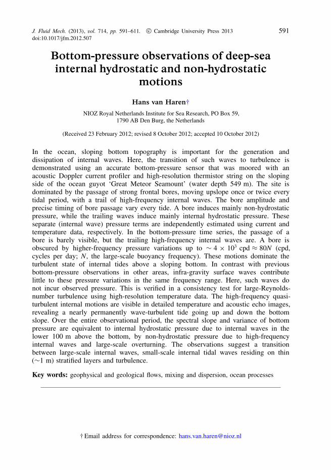
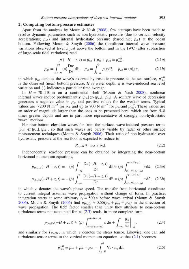
FIGURE 1. Location of mooring (∗) near the top of Great Meteor Seamount. Bathymetryis computed from 1′ topography, an update from Smith & Sandwell (1997). Depth contourlines are every 500 m for [500, 4500] m. Above the east–west directed slope, thermistor stringextent (vertical bar) and upper acoustic current meter (∗) are indicated.

The reason for adding stress tensor terms is that, above sloping topography, turbulentoverturning is expected besides highly nonlinear internal waves. Unfortunately,resolution of all terms in (2.4) and (2.5), including establishment of precise phaserelationships, requires more instrumentation than presently employed. However, as willbe reasoned in § 3, and as partially has been done above, the magnitudes of differentpressure terms can be established with the present set-up to within a factor of 2for internal waves and for the larger turbulent overturns. Following the atmosphericobservations described in § 1.2, it is not expected to establish phase relationshipsbetween different pressure estimates that are mainly due to turbulence, commensuratewith its (still unknown) three-dimensional character.

3. DataGreat Meteor Seamount (GMS) rises up to 300 m from the surface in an otherwise

relatively flat, 5000 m deep Canary Basin in the North-East Atlantic Ocean. Thedominant driving force of motions in this part of the ocean is the semidiurnal tide.About 250 m below GMS’s summit, a 3 m × 2 m × 1.7 m sturdy bottom landerwas moored at 549 m for 18 days in May–June 2006 (figure 1; see table 1 formooring details). The mooring is well above the depth range of Mediterraneanoutflow and therefore temperature is an adequate tracer for density variations, witha tight relationship δρ = (−0.101±0.002)δT kg m−3 ◦C−1 as established from multipleconductivity–temperature–depth (CTD) casts in the vicinity of the mooring.

A deep-water SBE53 bottom-pressure recorder was mounted inside the lander,attached to its central axis. The recorder is equipped with a Digiquartz crystal,temperature-compensated pressure sensor that has an absolute accuracy of 10−4 offull scale. The accurate (0.002 ◦C), high-resolution (0.0001 ◦C) temperature sensor andinternal temperature compensation ensure a residual temperature sensitivity in pressuredata <3.5 N m−2 ◦C−1 in the range between 0 and 20 ◦C. The bottom-pressure


Latitude 30◦00.052′NLongitude 28◦18.802′WWater depth 549 mLocal bottom slope 4± 1◦Moored period 21/05–08/06 2006Pressure sensor SBE53, 0.33 Hz, 1.70 m above the bottomCurrent meter Nortek AquaDopp, 0.2 Hz, 2.50 m above the bottomAcoustic Dopplercurrent profiler

RDI 300 kHz, 0.53 Hz, lowest bin 4 m above the bottom,80×1z= 1 m

Thermistor string NIOZ3, 1 Hz, lowest sensor 0.5 m above the bottom,101×1z= 0.5 m

Current speed 0–0.5 m s−1

N,N1max 50, 600 cpd (cycles per day)

TABLE 1. Details of bottom-lander mooring near the top of Great Meteor Seamount.

sensor has an absolute accuracy of ∼20 N m−2 and a resolution of 3 N m−2 forthe 0.33 Hz sampling rate. These values are adequate to measure O(10–102) N m−2

non-hydrostatic and internal hydrostatic pressure variations induced by, for example,internal waves, which, moreover, are found at much lower frequencies than thesampling frequency of 0.33 Hz. For small-scale internal waves near the buoyancyperiod of 600 s, random sampling errors are <4 N m−2.

From tilt-sensor information it is inferred that the 200 kg bottom lander vibratesslightly under strong turbulence. This causes very high-frequency (>0.1 Hz) pressurevariations (‘noise’) up to 10 N m−2. These vibrations do not influence the pressureobservation of the relevant processes, as no significant coherence has been foundbetween tilt and pressure variations (see further § 4).

In addition to the pressure sensor, a Teledyne RDI 300 kHz acoustic Doppler currentprofiler (ADCP), sampling at a rate of 0.5 Hz, and a 1.5 MHz single-point acousticcurrent meter (Nortek AquaDopp), sampling at 0.2 Hz, are mounted in the lander. Theclosest current measurement to the sea floor was by the AquaDopp, at 2.5 m above thebottom. The ADCP ranged from 4 to ∼50 m above the bottom. It only rarely reachedto its maximum range of 85 m above the bottom when sufficient acoustic scattererswere floating by. A string of 100 NIOZ high-sampling-rate thermistors (van Harenet al. 2009) measured temperature precisely (<0.001 ◦C) at 1 Hz and at 0.5 m verticalintervals between 0.5 and 50 m above the bottom. Directly above the string another0.2 Hz sampling AquaDopp was mounted just below the top buoy.

Although instrumentation and mounting should be adequate to resolve internal waveturbulence pressure variations, estimates of the pressure terms in (2.1), (2.3), (2.4)or (2.5) all have some shortcomings. Precise knowledge of instrumental qualities isnecessary prior to analysing the observations. ADCP data are relatively noisy dueto a general lack of scatterers and reflections off thermistors in the observationalarea. These reflections are easily identifiable, but reduce the number of good data.More generally, current data are only obtained in the range [2.5, 80] m above thebottom in nearly 550 m water depth. Thus we lack data very close to the bottom,which somewhat hampers estimate (2.4), and we lack surface current data andhence estimates of peh, although they are expected to be small. The ADCP usesfour slanted beams and gives current estimates over horizontal surface areas withdiameters between 10 and 60 m, which approximate the smallest wave scales, therebyunderestimating their current values in estimates like pnh (Moum & Smyth 2006).

598 H. van Haren

Even though we only resolve about 10 % of the water column, the present dataset is not as limiting as it seems because most significant contributions to bottompressure are expected from motions close to the bottom (Thomas & Bull 1983), exceptfor hydrostatic surface tides. Following the reasonable assumptions for internal wavepressure terms made in Moum & Smyth (2006), one can state that: (i) for linear butalso smoothly varying nonlinear waves, advection terms contribute <10 % to Dw/Dt,so that local time derivatives can be used to estimate pnh, at least for z > 10 m abovethe bottom, which is resolved here; (ii) the lack of peh estimates will not alter thebottom-pressure effects of near-bottom solibore elevation wave types, which are barelynoticeable at the surface 550 m above; and (iii) part of the investigation here includesa comparison between pih and pnh estimates with p−H

obs . This investigation will includethe effects of near-bottom nonlinear and overturning waves and their extent into thewater column up to 50 m above the bottom. It is hypothesized that pnh may be moreaffected than pih by a lack of observations higher up in the water column, since thevertical extent of stratified thin layers can be much smaller than that of their associatedvertical motions even though the range of their coherency is the same (e.g. van Haren2009).

4. Observations4.1. General overview observations

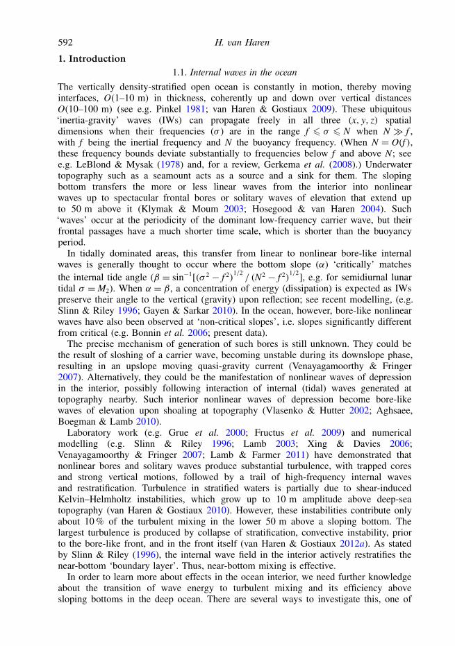
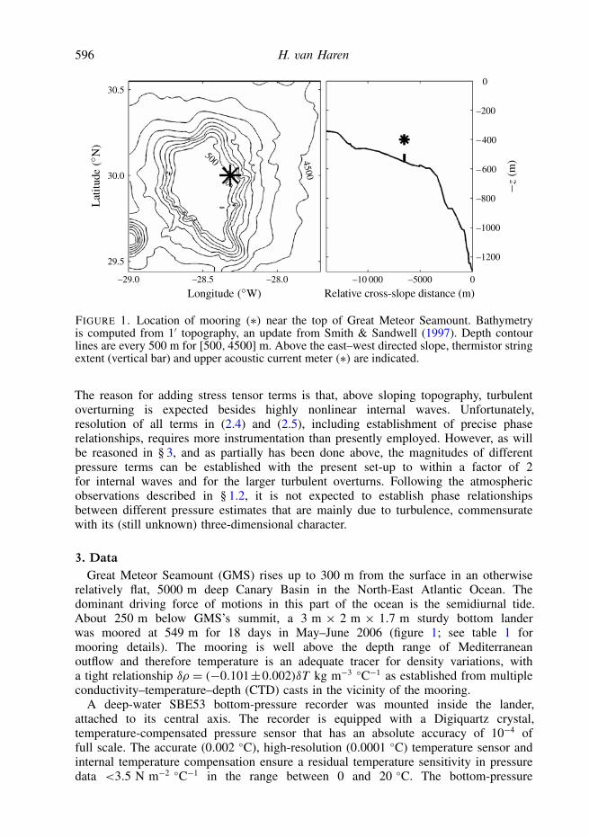
Above the sloping side of GMS, a total near-bottom temperature record shows adominant semidiurnal tidal cycle and its spring–neap modulation (figure 2a, purple).In more detail, the temperature variations with time are not sinusoidal in shape, butmore asymmetric. Removal of tidal harmonics and lower-frequency variations revealsthe sharp nonlinear part of the asymmetric motions (figure 2a, black). Once every tidalcycle a major front passes the sensors. The front leads the upslope cooling tidal phase,but the strength of the front and its precise arrival time at a fixed position vary by upto ∼10 % every tidal cycle. They are thus not modulated by spring–neap variation andthe same holds for occasional secondary fronts following a few hours later. In addition,less spiked and smaller high-frequency variations are more persistent throughout therecord, with largest amplitudes mostly in the down-going warming tidal phase justprior to the arrival of the major front.

In comparison, the observed total near-bottom pressure record shows a similarspring–neap modulated semidiurnal tidal dominance (maximum 0.9 m range), mainlydominated by the surface barotropic tide, and more sinusoidal in appearance (figure 2b,purple) than T variations. In contrast, the pressure part without tidal harmonics andlower-frequency variations, after using double elliptic band-pass filters (figure 2b,black; see figure 3 for filter bounds) is more continuously noise-like in time thanits temperature equivalent. This featureless high-pass filtered pressure record p′ showsonly a weak fortnightly modulation about 5 days out of phase with the modulationin the surface tide. The amplitudes of p′ are maximum 100 N m−2, more commonlyseveral tens of newtons per square metre.

If we further separate into three parts this tidally filtered bottom pressure, we findtidal (but not spring–neap) variation and peaked changes of variance with time in itslower-frequency portion (figure 2c, light blue). The number of spikes roughly equalsthat in T ′ (figure 2a), but they occur at different times. This lower-frequency portion isthe IWC band, in which the observed pressure spectrum falls off in frequency at a rateof log(pIWC)= c− (2.0± 0.3) log(σ ), with c a constant (figure 3, blue). It lies between


555.6

555.2

554.8

100

0

–100

pIWC pIWTN pIWTT

15

14

13

12

11

10

0.05

0

–0.05

10

15

5

142 144 146 148 150 152 154 156 158

30

15

0

Yearday 2006

(a)

(b)

(c)

FIGURE 2. Overview of two-and-a-half weeks of time series data. (a) Near-bottom totaltemperature at 1.7 m above the bottom (purple), and its high-pass filtered variations (black;frequencies σ > 7 cpd; amplitude multiplied by a factor of 20; scale to right, and arbitrarilyoffset vertically). (b) As panel (a), but for pressure. (c) One-hour averaged, band-pass filtered(cf. figure 3 for filter bounds) near-bottom pressure amplitudes: |pIWC| (light blue), |pIWTN |(green), and |pIWTT | (red). Also shown is wind speed (purple; scale to right) measured every60 s on board R/V Pelagia and corrected for the ship’s speed.

tidal harmonics and the band containing the internal wave transition to turbulenceIWT.

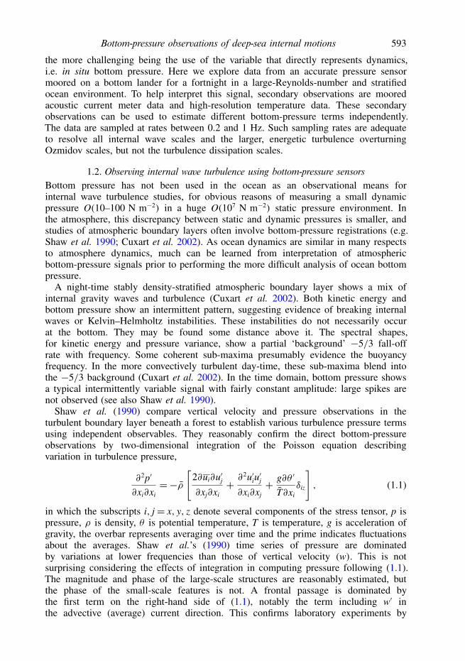
Although acceleration spectra (figure 3, purple), estimated using ADCP tilt sensordata, show approximately the same slope as observed bottom pressure in the IWCband, their variance is two orders of magnitude smaller. In the very high-frequencynotch of bottom pressure (∼ 6 × 103 cpd), the two spectra match in variance. This isevidence only in that frequency range of some influence of lander movements on thebottom-pressure observations (by limiting the depth of the notch).

The above IWC bounds do not coincide with the classic IW bounds under thetraditional approximation [f ,N],= [1, 50] cpd here. At the low-frequency side, this isdue to the contribution of tidal harmonics to bottom pressure and to weakly stratifiednear-homogeneous layers forcing N to approach f occasionally. At the high-frequencyside, it is due to small-scale layering in density. The 90th percentile value of buoyancyfrequency computed over small vertical scales of 1z = 1 m is set to N1. It coincideswith the kink in spectral slopes that indicates the transition between IWC and IWT.The N value calculated over 1z = 1 m varies over two frequency decades, a broadband that thus easily covers the spectral IWC range.

600 H. van Haren

106

102

10–2

10–6

100 102 104

M8

–1

–2

Tilt

IWCT

f M2

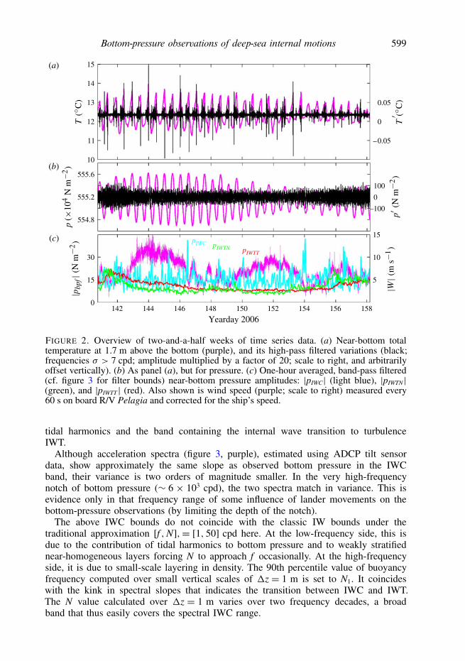
FIGURE 3. Spectra of observed near-bottom pressure (blue) in comparison with near-bottomtemperature (black; arbitrarily offset vertically) and its pass-band filter bounds (same coloursas in figure 2c; offset vertically). Also shown is the vertical acceleration inferred fromADCP’s tilt data in units of pressure (purple). Several buoyancy frequencies are indicated:1z = 1 m minimum, mean, 90th percentile of 1 m, and 1 m maximum, by blue bars indescending order. Spectral slopes are given (purple), which may mimic internal waves(σ−2, solid), stratified turbulence (σ−3, solid, repeated in IWTT range), inertial (turbulent)convective subrange (σ−5/3, dashed, repeated in IWTT range) and low-wavenumber pressureturbulence transferred to frequency range (Gotoh & Fukayama 2001) (σ−7/3, dashed).

The value of N1 is found to extend well into IWT (figure 3); 10 % of the high-frequency ‘internal wave’ thin-layer buoyancy frequencies are found in this range.Here, we use the extreme N1max to separate this band at the non-significant maximumof the IWT bulge into a ‘buoyancy frequency internal wave/turbulence part’ IWTN

and a pure ‘turbulence’ part IWTT . This separation frequency also coincides with thetransition of the near-bottom T spectrum (figure 3, black) from a σ−7/3 slope to aσ−5/3 slope, when we ignore the statistical significance and when we take into accountthat spectra are plotted logarithmically so that we should give more emphasis to higherthan to lower (neighbouring) values. (Compared to χ 2 noise distribution of statisticalsignificance, most of the T spectrum, excluding tidal harmonics, lies within a −2± 0.3fall-off rate.) A −5/3 slope is commonly attributed to high-wavenumber ‘Kolmogorov’turbulence scaling, a −7/3 slope to low-wavenumber inertial range turbulence, butso far for simulated ‘theoretical’ pressure mainly (Gotoh & Fukayama 2001; Tsuji &Ishihara 2003), rather than for temperature and in a different frequency range thanobserved here.

In contrast to the T spectrum, the p spectral slope in the IWC band log(pIWC) ≈−2 ± 0.1, which confirms the notion that internal waves dominate the inertialturbulence range in p−H

obs . At frequencies higher than those of the IWC, the flat bulgemaximum part of the p spectrum and especially its −1 and more steeply sloping high-frequency roll-off rate for σ > N1max is dominated by turbulence. This is provisionallyconcluded from its similarity with high-Reynolds-number free stream turbulence pspectra that roll off from a flat bulge at rates between −1.0 and −1.6 before steeper


f M2

–2

106

102

10–2

100 102 104

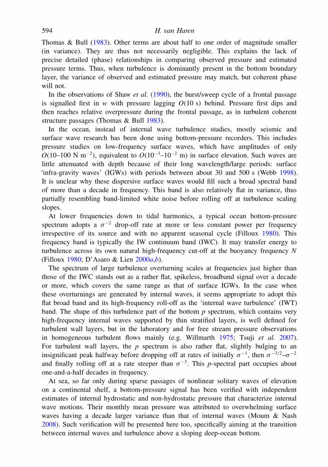
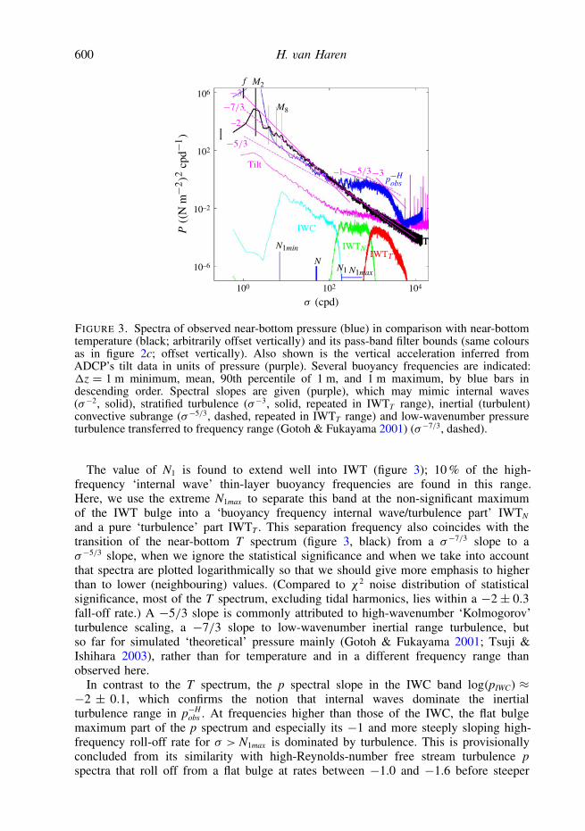
FIGURE 4. Spectra of observed near-bottom pressure (blue, same as in figure 3, given herefor reference) in comparison with several internal wave pressure estimates following (2.1)and (2.3): pnh (red, cut-off at border IWTN/IWTT ∼ N1max) inferred from AquaDopp’s near-bottom vertical current, which are verified to be comparable with ADCP data from twodepths, and assumed to be valid for a 50 m vertical range; pih (black) inferred from NIOZthermistor string temperature data. Bottom pressure is also estimated from AquaDopp near-bottom horizontal current data pDu/Dt (green, using constant c = 0.5 m s−1, same cut-off aspnh). See text for definitions and precise calculations. Slopes as in figure 3.

roll-off (Willmarth 1975; Tsuji et al. 2007). Turbulence may be associated with thedominant tidal motions (see also discussion in § 5), thereby partially explaining thefortnightly modulation in IWT (figure 2c), but surface infra-gravity waves above deepwater far from coasts are unlikely to be so. Variance in none of the three band-passfiltered pressure parts is significantly coherent with the local wind speed (figure 2c,purple), which predominantly shows a diurnal and a 6-day periodicity. Occasionally,IWC and IWTN modulations match over a short period with |W| and generally nottogether at the same time, and their mutual correlation is found to be insignificant overthe entire period of 18 days.

The difference in the spectral slopes of temperature and pressure is attributable totheir different measurement: pressure acts like an integrator of the (wave) motionsabove it. This difference is independently demonstrated by integrating temperature overthe full 50 m above the bottom of the thermistor observations. This results in an(internal wave) estimate of pih. When transferring temperature to density variations andassuming that they represent the lower 100 m of the water column commensurate withthe typical internal (tidal) wave vertical coherence scales and the extent of associatedturbulent overturns (van Haren & Gostiaux 2012a), one finds (figure 4, black) the σ−2

slope and a near-perfect match. This is well within the statistical 95 % significancebounds, with p−H

obs in the IWC (between N1min and N1).The same IWC slope and approximately the same level, although slightly less in

variance by about 30 %, which is still larger by a factor of 2 than the reduction foundby Moum & Smyth (2006), is independently obtained from the pressure estimate (2.3),pDu/Dt component, using AquaDopp’s along-slope currents at 2.5 m above the bottom

602 H. van Haren

and assuming a constant phase speed (figure 4, green). This spectrum changes slopetowards instrumental noise approximately at N1.

For σ > N1, lower-frequency dominant pih becomes overwhelmed by pnh (figure 4,red), which is estimated here from AquaDopp’s near-bottom vertical motions asa representative of the range of thermistor observations. (This is probably anoverestimate, because of the instrumental noise in w, especially in the range for IWTT .This noise is thus largely filtered out here. In § 4.2 we estimate pnh using ADCP data,which are only good over short sections of time but not over the entire record at everydepth.)

For the two-week mean in figure 4 we thus conclude that observed bottom pressureis dominated by pih in the IWC (Rp,−H � 1; from (2.2)) and by pnh and turbulentstress in the IWT (Rp,−H � 1). Below, the contributions of the different terms areinvestigated for some periods in detail. Owing to the shortness of these periods, wefocus on motions near the local buoyancy frequency or highly nonlinear waves. Thesemotions will thus be mainly non-hydrostatic (Rp,−H � 1) and potentially Rp,−H = 1 forfreely propagating internal waves near the small-scale buoyancy frequency N1, whichindicates the transition between pih and pnh dominance (figure 4).

4.2. Detailed observationsThe passage of an upslope frontal bore (figure 5; 0.6 h detail) is accompanied,shortly before and after, by strong downward and upward vertical motions exceeding0.1 m s−1 (figure 5a) and by a single very strong (40 dB above ambient level) echomoving upwards from the bottom (figure 5b). These observables are associated withsediment resuspension extending over 40 m above the bottom within minutes. Thefront, delineating the highly nonlinear end of the downslope moving tidal warmingphase, is trailed by a series of ‘free’ waves having about the local buoyancy period.The trailing waves are supported by the thin-layer stratification between the warmdownslope moving water above and colder upslope moving water below (figure 5c).Such a strong bore occurs here approximately once every sloshing tidal cycle, butsimilar bores, one including 24 h run-up, have been reported governed by sloshingsub-inertial current systems in other areas (Hosegood & van Haren 2004; Grue &Sveen 2010).

Although the trailing high-frequency waves characterized by typical 600–900 speriods and 10–20 m amplitudes are discernible in bottom pressure and more clearlyin temperature (figure 5c), the detailed temperature image is dominated by ruggedquasi-turbulent motions. Such turbulent motions are not only observed around the(curved) front, but also scattered around the image in small details. The apparent‘periods’ of these turbulent motions are far shorter than the smallest buoyancy periodcomputed (2π/N1max ∼ 150 s), as they reach down to periods O(10 s).

Such short-period variability is dominant in the high-frequency bottom-pressurerecord (figure 5c, purple; arbitrary scale), and it can be more or less matchedwith variations in the temperature image in the same figure. This variability is soomnipresent that the frontal bore does not stand out very clearly in p−H

obs . A dip ofabout −50 N m−2 is measured at the time of the bore’s passage (more clearly visiblein figure 5e, purple; the same record as in figure 5c), but many such dips or spikesoccur in the record. From a bottom pressure perspective the frontal bore is not anexceptional phenomenon.

The bore is more clearly visible in the separate estimates of (internal wave) bottompressure: all show a dip (figure 5e, blue pDv/Dt that matches very well the dip inpurple p−H

obs ) or a front (figure 5d,e, red pnh, black pih, green pDu/Dt) of 20–50 N m−2


500

520

540

500

520

540

500

520

540

50

0

–50

50

0

–50

146.58146.57 146.59

Yearday 2006

0.05

0

–0.05

20

0

–20

14

13

12

600 s

(a)

(b)

(c)

(d )

(e)

D D

D D

FIGURE 5. Example of relatively large IWC contributions to bottom pressure and a large,backwards breaking, upslope moving bore and its trail in a 0.6 h detail. (a) Depth–timeseries of ADCP’s raw vertical motions. The horizontal lining in the lower half of the figureand the noise speckles higher up are due to artificial reflectance off T sensors. (b) ADCP’srelative echo intensity. See remark about panel (a) on the influence of thermistors on acousticdata. (c) Temperature measured at 1 Hz, 0.5 m vertical intervals. The bottom-pressure record(purple) IWC + IWTN + IWTT band-pass filtered is also shown (arbitrary scale). (d) Theband-pass filtered observed bottom pressure (purple) IWC + IWTN + IWTT plotted withpnh (red) and pih (black) estimated over the range of thermistors, and with IWC + IWTNband-pass filtered pnh (light blue). (e) The band-pass filtered observed bottom pressure(purple) IWC + IWTN + IWTT compared with independent near-bottom (1.7 m above thebottom) pressure estimates of cross-slope pDv/Dt (purple) and along-slope pDu/Dt (green) usinga constant c= 0.2 in (2.3).

in amplitude around the bore’s passage. As already noted in their spectra, pnh and pih

have approximately the same range of variation but a completely different character:pnh is dominated by higher-frequency variations compared to pih. Around the bore’spassage, their signs are commensurate with those for elevation waves (Moum & Smyth2006): they are opposite in sign and roughly cancel each other out here for motions atσ ≈ N1. Note that in this case pnh is computed from integrating the ADCP’s verticalmotions (figure 5a) approximately over the same range as the thermistors, except forthe lower 4 m (no ADCP data) and upper 5 m of the thermistors’ range (some lackof scatterers for ADCP). The exclusively upslope movement of the frontal bore is

604 H. van Haren

well retrieved, as the dips in the pDv/Dt term and observed bottom pressure are nearlyindistinguishable (figure 5e).

Also, around the time of the bore’s passage, including the first large overturn on day146.5785, pnh shows more variance than in the rest of the tidal period. The front marksa transition from smooth (low-frequency IWC variance dominated) to slightly morenoisy (high-frequency IWC increased) pih (figure 5d). Away in time from the bore’spassage, after day 146.61, the slower (IWC) variations in p−H

obs (purple) are not so wellmimicked by the independent estimates of pressure terms (not shown). Apparently,variations higher up in the water column are more important in this example whenstratification moves out of the range of the sensors, especially in pih. Although exactphase correspondence is lacking, the intensity (amplitude and variation with time) ofhigher-frequency IWT motions is comparable in pnh (red) and p−H

obs (purple) (figure 5d).The independent estimate pDv/Dt (figure 5e, blue) shows marginal IWT variations,

and generally fails to describe the IWC as in p−Hobs (purple). An exception is around

the time of the bore passage, when motion is strictly up the slope. This lack ofcomparison for IWC is partially compensated in pDu/Dt (green) further in the record,which better follows typical IWC 600–900 s periodic variations, but not entirelybecause near-bottom currents are just not well measured, not even by the AquaDoppat 2.5 m above the bottom. So, while high-frequency IWC and low-frequency IWT, i.e.motions at σ ≈ N1, including a frontal passage, are comparable in size for pnh and pih

with opposite signs, the exclusively upslope moving front is best observed in pDv/Dt

with a near-perfect match with p−Hobs (figure 5e). In contrast, pDu/Dt(figure 5e, green)

describes pnh (IWC + IWTN part; figure 5d, light blue). As noted from the spectra,turbulence dominates (the IWT part of) p−H

obs and it is recalled that the estimates (2.1)and (2.3) are for waves.

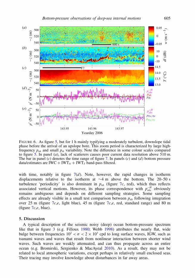
The lack of bottom current measurements is somewhat more problematic during aperiod prior to a bore arrival, when stratification reaches very close to the bottomand low amounts of scatterers are found higher up (figure 6; 1 h detail). This periodseems to be dominated by high-frequency local apparent vertical mode-2 internal‘motions’ close to the local buoyancy period of ∼450 s (figure 6c). Vertical currentsare weak, indicative of a lack of large vertical coherence, and the stratification ismainly moved by quasi-turbulent motions. As before, pnh (figure 6d, red) mimicswell the observed bottom pressure (purple) in IWT variance, whereas here weak pih

(figure 6d, black) is only marginally retrieved in p−Hobs (purple). The pDv/Dt (figure 6e,

blue) and pDu/Dt (figure 6e, green) mainly describe IWC rather than IWT, with areasonable comparison between pDu/Dt and observed IWC pressure in the secondhalf of the period. Observed IWT pressure variations are visible in both p−H,obs andshort-term ‘turbulent’ temperature variations (figure 6c). These variations thus do notreflect direct surface wave variations, as even the small-scale turbulent overturningtemperature interface variations have amplitudes of several metres in the vertical,rather than O(10−3 m)∼= O(10 N m−2) for IGW surface waves.

In an arbitrary, more detailed zoom (figure 7), near-buoyancy frequency internalwaves of 500 s period (figure 7a) support the shorter (down to 20 s) period motions,also away from the interface that carries them (local maximum buoyancy period inthe interface equals 450 s). In the weaker stratified layer, these ‘waves’ do not losecoherency completely, amid the overturns, even though the local stratification doesnot support them as freely propagating waves. At the interface and also away fromit, 20–50 s period motions occur often, albeit intermittently in time, having typical0.5–1 m amplitudes (more clearly visible in detail in figure 7b,d). The dominantperiodicity in p−H

obs (purple) is 20–50 s, and it compares with isotherm variation


500

520

540

50

0

–50

50

0

–50

600 s

F7

500

520

540

500

520

540

143.96

Yearday 2006143.95 143.97

0.05

0

–0.05

10

0

–10

14.0

14.5

13.5

13.0

(a)

(b)

(c)

(d )

(e)

D D

D D

FIGURE 6. As figure 5, but for 1 h mainly typifying a moderately turbulent, downslope tidalphase before the arrival of an upslope bore. This zoom period is characterized by large high-frequency pnh and small pih variability. Note the difference in some colour scales comparedto figure 5. In panel (a), lack of scatterers causes poor current data resolution above 510 m.The bar in panel (c) denotes the time range of figure 7. In panels (c) and (d) bottom pressuredata/estimates are IWC+ IWTN + IWTT band-pass filtered.

with time, notably in figure 7(d). Note, however, the rapid changes in isothermdisplacements relative to the isotherm at ∼4 m above the bottom. The 20–50 sturbulence ‘periodicity’ is also dominant in pnh (figure 7c, red), which thus reflectsassociated vertical motions. However, its phase correspondence with p−H

obs obviouslyremains ambiguous and depends on different sampling strategies. Some samplingeffects are already visible in a small test comparison between pnh following integrationover 25 m (figure 7c,e, light blue), 45 m (figure 7c,e, red, standard range) and 80 m(figure 7c,e, blue).

5. DiscussionA typical description of the seismic noisy (deep) ocean bottom-pressure spectrum

like that in figure 3 (e.g. Filloux 1980; Webb 1998) attributes the nearly flat, widebulge between frequencies 102 < σ < 2× 103 cpd to long surface waves, IGW, such astsunami waves and waves that result from nonlinear interaction between shorter windwaves. Such waves are weakly attenuated, and can thus propagate across an entireocean (e.g. Bromirski, Sergienko & MacAyeal 2010). As a result, they may not berelated to local atmospheric variations, except perhaps in relatively small enclosed seas.Their tracing may involve knowledge about disturbances in far away areas.

606 H. van Haren

143.944 143.948 143.952

Yearday 2006

hab

(m)

hab

(m)

50

30

10

–10

60 s

12

10

6

2

8

4

12

8

4

20

0

–20

143.946 143.947 143.948 143.950 143.951 143.952

503010

–10

(a)

(b)

(c)

(d )

(e)

150 s

FIGURE 7. Near-bottom 1200 s detail of figure 6, highlighting 17–50 s time scale turbulent‘wave-like motions’. (a) Temperature contours between [13.3, 14.0] ◦C in 0.1 ◦C intervals.Also shown is the bottom-pressure record (purple), differently band-pass filtered (IWC +IWTN + IWTT , solid; IWC+ IWTN , dash-dotted; IWC, line with circles); scale to right. Barsindicate 250 s detail panels to left (b,c) and right (d,e) columns. (b) Detail of panel (a), inwhich (inverse) IWC + IWTN + IWTT bottom pressure does not well match the temperaturecontour variations. (c) Bottom pressure as in panel (a) (purple), compared with threeestimates of pnh (red, as before; and light blue, blue for height ranges above the bottomas indicated) and pih (black, multiplied by a factor of 10 as if governed by the entire watercolumn). (d,e) As panels (b,c), but for period in which (inverse) bottom pressure partiallymatches temperature contour variations.

Nonetheless, for a number of reasons, such surface waves cannot force turbulenceabove sloping topography as observed here, even though the dominant bottom-pressurevariations fall within the same frequency range. First, the fortnightly spring–neapmodulation as observed here is not a result of an interaction between distant ‘storm-modulated’ surface waves (van Haren 2011). Even though tidal (high and low water)modulation of surface infra-gravity waves has been reported for shallow watersclose to shore (Okihiro & Guza 1995), this cannot cause a dominant spring–neapmodulation out in the open ocean, where waves from multiple shores with differenttidal phases combine. Second, one cannot dismiss the energy input of internal tides,into higher harmonics and into eventual strongly nonlinear motions, without neglectingthe transition to turbulence as in overturning motions observed here. (It is noted thatsome nonlinear regimes exist in which the motion is not turbulent (Grue 2005).)Third, surface IGWs do not create the observed highly nonlinear frontal bore, whichis density-driven, nor Kelvin–Helmholtz overturning, which is shear-driven. The latteroccur in the downslope phase and have a 20–50 s periodicity, which is far smallerthan the smallest internal wave period (van Haren & Gostiaux 2010). Fourth, if surfaceIGWs would create ‘turbulence’ IWT, they should also do so in the ocean interior,


not exclusively above sloping topography. This is not observed in similar detailedtemperature observations far from boundaries in the Canary Basin, which show weaklyturbulent, smooth internal waves (van Haren & Gostiaux 2009).

Recent estimates of turbulence parameters have been made for the dynamic GMSsloping boundary by means of reordering all of the 1 Hz sampled temperature-sensor profiles using the method proposed by Thorpe (1977). These estimates yieldhighly varying turbulence dissipation rates between 10−9 < ε < 10−4 W kg−1, witha depth–time mean of 〈ε〉 = (1.5 ± 0.7) × 10−7 W kg−1 (van Haren & Gostiaux2012a). The variance of depth-averaged dissipation rates has been compared withthe variance of various pressure terms, which resulted in a coherent signal, with180◦ phase difference, at 75 % significance level at semidiurnal and its first harmonicfrequencies. Van Haren & Gostiaux (2012a) demonstrate that the spectrum of heatflux transits from the canonical internal wave −2 slope to the turbulence −5/3 slopeat the frequency where the eddy diffusivity and the pressure spectra transit fromtheir IWC slope to the IWT bulge. Furthermore, the spectral shape of variance andparticular time series of intermittent turbulence pressure and vertical currents resembleturbulence observations in the atmospheric boundary layer. The present observed lackof precise phase correlations does not imply a lack of correspondence betweensource (internal waves) and turbulence dissipation as was intrinsically proven formeasurements in the turbulent atmospheric boundary layer (Cuxart et al. 2002). Thedifferent wave pressure terms pih (IWC mainly) and pnh (IWT mainly) show spectralshapes and variances in their respective frequency bands that are comparable withthose of p−H

obs . It implies that the vertical length scale of integration (50–100 m abovethe bottom) is adequate, in most instances, especially for estimating pnh. A future morecomplete data set should establish this more firmly.

The spectral shape of IWC, being self-similar in constant slope and variance(Filloux 1980; van Haren 2011), thus representing a saturated internal wave field, andIWT, with a varying bulge variance, are consistent with the internal wave turbulencemodel of D’Asaro & Lien (2000a,b). This model resembles the neutral atmosphericlaw-of-the-wall turbulence pressure spectrum (Willmarth 1975). However, we note thatthe present turbulence is partially generated in the interior, occasionally resulting in aturbulent bore moving up a sloping bottom, with relevance for sediment resuspension.

This difference in turbulence character is evidenced in a consistency test for law-of-the-wall turbulence, using 10 min intervals of figure 5. We fit ADCP velocity profileswith the model of a constant (bottom frictional shear) stress layer to obtain a frictionvelocity u∗ (Wyngaard 1973)

u(z)∝ u∗κ

ln z, (5.1)

with κ = 0.4 denoting the von Karman constant. Independently, u∗ is estimated usingthe above high-resolution thermistor string data. It is estimated under the rather crudeassumption of negligible buoyancy flux, so that the kinetic energy production matchesthe dissipation rate ε,

u3∗ = εκz. (5.2)

Although the two different estimates are found to be consistent to within a factorof 3, the law-of-the-wall model overestimates the friction velocity before and after thefront, and underestimates it during the frontal passage (figure 8). It is clear that atight logarithmic profile is not observed. Also, a two-fold log layer (‘modified law ofthe wall’), as in Perlin et al. (2005), is not observed here. These discrepancies with

608 H. van Haren

0.1 0.2 0 0.1 0.2 0 0.1 0.20

10

40

4

FIGURE 8. Law-of-the-wall turbulence test for three 10 min periods around the frontalpassage of figure 5. Dots indicate the ADCP-observed current magnitudes (with low biasedvalues due to reflection at thermistors removed). The red line is the log-linear best fit tothese data to provide a friction velocity following (5.1). The green dashed lines indicatehypothetical slopes (using arbitrary initial depths) for friction velocities independentlycomputed using (5.2) for z = 10 m from turbulence dissipation rates estimated using high-resolution thermistor string data (van Haren & Gostiaux 2012a).

models (5.1) and (5.2) may have to do with the boundary layer above a sloping bottombeing nearly always (re)stratified in density (figure 5) so that turbulence isotropy maynot be achieved, except perhaps very briefly during the passage of a turbulent bore.

A similar result is obtained after comparison of the turbulent part of the observedbottom pressure, pIWTT , with pressure independently estimated from dissipation ratesusing high-resolution temperature data between 0.5 and 50 m above the bottom(for the method, see van Haren & Gostiaux (2012a)). Under the assumption ofisotropic turbulence and high-Reynolds-number flows, Kolmogorov scaling yields atwavenumber k for the, presumably free stream rather than bottom or wall, pressurespectrum (Tsuji & Ishihara 2003)

Pp(k)∝ p2ε = Kpρ

2ε4/3kγp, γp =−7/3, (5.3)

in which Kp denotes a ‘universal constant’. Extensive (free stream pressure) laboratoryobservations were made by Tsuji & Ishihara (2003) up to Reynolds numberRe = UL/ν = 15 000, with kinematic viscosity ν ≈ 1.5 × 10−6 m2 s−1, and U and Lthe velocity and length scales of the flow. Their results yielded higher γp and smallerexponent of ε than in (5.3). They also found a linear dependence of Kp ∝ Re/150 andthey attributed their findings to non-isotropic turbulence. Here, restratification occursrapidly and continuously. As average U = 0.2 m s−1 and a typical L = 0.1–10 m, onehas Re ∼ 104–106, very large indeed. A fit of overall mean pε is made to mean pIWTT

(approximately mean pIWTN) using both (5.3) and γp =−4/3 as the mean of exponentsfound by Tsuji & Ishihara (2003). In the fitting, Kp(Re) and k (wavelength λ) areused as parameters, yielding best fits for the combinations λ = 10 m, Re = 5 × 106

and 3× 105, respectively, and λ= 50 m, Re= 1.1× 105 and 6× 104, respectively. TheReynolds numbers are in the expected high range. In figure 9, the time series pε (blue)provides a similar spring–neap variation compared to those of pIWTT (red) and pIWTN


Yearday 2006

pIWTT(pIWTN)

(pIWC)

30

15

0158142 146 150 154

FIGURE 9. As figure 2(c) without wind speed and with 10 h smoothed pressure estimatedfrom turbulence dissipation rate using high-resolution temperature data from 101 sensorsbetween 0.5 and 50 m above the bottom. Two parametrizations are used: p2

ε ∝ ε4/3 (dashedblue) following (5.3) as in Kolmogorov scaling for isotropic turbulence in high-Reynolds-number flows; and p2

ε ∝ ε13/12 (solid blue, γp = −4/3) following the mean exponential valuedetermined in laboratory turbulent flows (Tsuji et al. 2007). The empirical scaling values aregiven in the text.

(green). The pε has a more spiky character, and at times the comparison is betterwith the more variable time series of pIWTN and even pIWC (light blue) than pIWTT . Wedo not expect an improved comparison between the mid-boundary layer (25 m abovethe bottom) pε and the observed bottom pressure, as ongoing restratification preventsturbulence from being isotropic.

So, some correspondence is found with wall turbulence, for which a pressurespectrum as in IWC and IWT here has been found for the atmosphere (Willmarth1975). The 3 min bore passage comprises about 20 % of the total dissipation rate ina tidal period (van Haren & Gostiaux 2012b). However, turbulence is generated notonly by shear stress at the bottom, but also by convection in the interior. The totalamount of turbulence kinetic energy dissipated in the lower 50 m above the slopingbottom amounts to about a quarter of the total internal tidal energy conversion byGreat Meteor Seamount (van Haren & Gostiaux 2012b). It remains to be establishedwhether this is mainly due to (breaking) internal waves returning to their source.

6. ConclusionsAbove a large-scale ocean bottom topography, the variance of observed bottom

pressure is found to be equivalent to independent estimates of internal hydrostaticpressure due to freely propagating internal waves up to 100 m above the bottomat frequencies lower than the buoyancy frequency, and of non-hydrostatic pressurefollowing internal wave (breaking) turbulence in the lower 50 m above the bottom atfrequencies higher than the buoyancy frequency.

The internal wave turbulence non-hydrostatic pressure dominates over long surfacewave bottom pressure, which may be found in the same frequency band.

Internal wave bottom pressure is also verified by near-bottom horizontal current(variations), in along-slope direction mainly, except during the passage of an upslopemoving frontal bore that generates a clear dip.

The frontal pressure dip of only 50 N m−2 in directly observed bottom pressure isamid omnipresent, mainly non-hydrostatic, internal wave turbulence pressure, whichis found to be weaker in independent (non)linear wave pressure estimates using near-bottom current observations.

610 H. van Haren

As in the atmospheric turbulent boundary layer, precise phase relationships cannotbe established between observed bottom pressure and different (internal wave) pressureestimates, especially not at frequencies higher than the buoyancy frequency.

As it shows no spectral gap, the transition between internal waves and turbulence isconfirmed to be smooth.

AcknowledgementsI enjoyed the assistance of the crew of the R/V Pelagia. I am greatly indebted to

M. Laan for construction of the NIOZ thermistors and to L. Gostiaux for facilitatingthermistor data analysis. Instrumentation and research cruises were funded in part bythe Netherlands Organization for the Advancement of Scientific Research, NWO (largeinvestment program ‘LOCO’) and BSIK.

R E F E R E N C E S

AGHSAEE, P., BOEGMAN, L. & LAMB, K. G. 2010 Breaking of shoaling internal solitary waves.J. Fluid Mech. 659, 289–317.

BONNIN, J., VAN HAREN, H., HOSEGOOD, P. & BRUMMER, G.-J. A. 2006 Burst resuspension ofseabed material at the foot of the continental slope in the Rockall Channel. Mar. Geol. 226,167–184.

BROMIRSKI, P. D., SERGIENKO, O. V. & MACAYEAL, D. R. 2010 Transoceanic infragravity wavesimpacting Antarctic ice shelves. Geophys. Res. Lett. 37, L02502.

CUXART, J., MORALES, G., TERRADALES, E. & YAGUE, C. 2002 Study of coherent structuresand estimation of the pressure transport terms for the nocturnal stable boundary layer.Boundary-Layer Meteorol. 105, 305–328.

D’ASARO, E. A. & LIEN, R.-C. 2000a Lagrangian measurements of waves and turbulence instratified flows. J. Phys. Oceanogr. 30, 641–655.

D’ASARO, E. A. & LIEN, R.-C. 2000b The wave–turbulence transition for stratified flows. J. Phys.Oceanogr. 30, 1669–1678.

FILLOUX, J. H. 1980 Pressure fluctuations on the open-ocean floor over a broad frequency range:new program and early results. J. Phys. Oceanogr. 10, 1959–1971.

FRUCTUS, D., CARR, M., GRUE, J., JENSEN, A. & DAVIES, P. A. 2009 Shear-induced breaking oflarge internal solitary waves. J. Fluid Mech. 620, 1–29.

GAYEN, B. & SARKAR, S. 2010 Turbulence during the generation of internal tide on a critical slope.Phys. Rev. Lett. 104, 218502.

GERKEMA, T., ZIMMERMAN, J. T. F., MAAS, L. R. M. & VAN HAREN, H. 2008 Geophysicaland astrophysical fluid dynamics beyond the traditional approximation. Rev. Geophys. 46,RG2004.

GOTOH, T. & FUKAYAMA, D. 2001 Pressure spectrum in homogeneous turbulence. Phys. Rev. Lett.86, 3775–3778.

GRUE, J. 2005 Generation, ppropagation and breaking of internal solitary waves. Chaos 15, 037110.GRUE, J., JENSEN, A., RUSAS, P.-O. & SVEEN, J. K. 2000 Breaking and broadening of internal

solitary waves. J. Fluid Mech. 413, 181–217.GRUE, J. & SVEEN, J. K. 2010 A scaling law of internal run-up duration. Ocean Dyn. 60,

993–1006.HOSEGOOD, P. & VAN HAREN, H. 2004 Near-bed solibores over the continental slope in the

Faeroe–Shetland Channel. Deep-Sea Res. II 51, 2943–2971.KLYMAK, J. M. & MOUM, J. N. 2003 Internal solitary waves of elevation advancing on a shoaling

shelf. Geophys. Res. Lett. 30, 2045.LAMB, K. G. 2003 Shoaling solitary internal waves: on a criterion for the formation of waves with

trapped cores. J. Fluid Mech. 478, 81–100.LAMB, K. G. & FARMER, D. 2011 Instabilities in an internal solitary-like wave on the Oregon shelf.

J. Phys. Oceanogr. 41, 67–87.


LEBLOND, P. H. & MYSAK, L. A. 1978 Waves in the Ocean. Elsevier.MOUM, J. N. & SMYTH, W. D. 2006 The pressure disturbance of a nonlinear internal wave train.

J. Fluid Mech. 558, 153–177.MOUM, J. N. & NASH, J. D. 2008 Seafloor pressure measurements of nonlinear internal waves.

J. Phys. Oceanogr. 38, 481–491.OKIHIRO, M. & GUZA, R. T. 1995 Infragravity energy modulation by tides. J. Geophys. Res. 100,

16 143–16 148.PERLIN, A., MOUM, J. N., KLYMAK, J. M., LEVINE, M. D., BOYD, T. & KOSRO, M. H. 2005 A

modified law-of-the-wall applied to oceanic boundary layers. J. Geophys. Res. 110, C10S10.PINKEL, R. 1981 Observations of the near-surface internal wavefield. J. Phys. Oceanogr. 11,

1248–1257.SHAW, R. H., PAW, K. T., ZHANG, X. J., GAO, W., DEN HARTOG, G. & NEUMANN, H. H.

1990 Retrieval of turbulent pressure fluctuations at the ground surface beneath a forest.Boundary-Layer Meteorol. 50, 319–338.

SLINN, D. N. & RILEY, J. J. 1996 Turbulent mixing in the oceanic boundary layer caused byinternal wave reflection from sloping terrain. Dyn. Atmos. Oceans 24, 51–62.

SMITH, W. H. F. & SANDWELL, D. T. 1997 Global seafloor topography from satellite altimetry andship depth soundings. Science 277, 1957–1962.

THOMAS, A. S. W. & BULL, M. K. 1983 On the role of wall-pressure fluctuations in deterministicmotions in the turbulent boundary layer. J. Fluid Mech. 128, 283–322.

THORPE, S. A. 1977 Turbulence and mixing in a Scottish loch. Phil. Trans. R. Soc. Lond. A 286,125–181.

TSUJI, Y., FRANSSON, J. H. M., ALFREDSSON, P. H. & JOHANSSON, A. V. 2007 Pressurestatistics and their scaling in high-Reynolds-number turbulent boundary layers. J. Fluid Mech.585, 1–40.

TSUJI, Y. & ISHIHARA, T. 2003 Similarity scaling of pressure fluctuation in turbulence. Phys. Rev.E 68, 026309.

VAN HAREN, H. 2009 High-frequency vertical current observations in stratified seas and ocean. Cont.Shelf Res. 29, 1251–1263.

VAN HAREN, H. 2011 Internal wave-turbulence pressure above sloping sea bottoms. J. Geophys. Res116, C12004.

VAN HAREN, H. & GOSTIAUX, L. 2009 High-resolution open-ocean temperature spectra. J. Geophys.Res. 114, C05005.

VAN HAREN, H. & GOSTIAUX, L. 2010 A deep-ocean Kelvin–Helmholtz billow train. Geophys. Res.Lett. 37, L03605.

VAN HAREN, H. & GOSTIAUX, L. 2012a Detailed internal wave mixing above a deep-ocean slope.J. Mar. Res. 70, 179–197.

VAN HAREN, H. & GOSTIAUX, L. 2012b Energy release through internal wave breaking.Oceanography 25 (2), 124–131.

VAN HAREN, H., LAAN, M., BUIJSMAN, D.-J., GOSTIAUX, L., SMIT, M. G. & KEIJZER, E. 2009NIOZ3: independent temperature sensors sampling yearlong data at a rate of 1 Hz. IEEE J.Ocean. Engng 34, 315–322.

VENAYAGAMOORTHY, S. K. & FRINGER, O. B. 2007 On the formation and propagation ofnonlinear internal boluses across a shelf break. J. Fluid Mech. 577, 137–159.

VLASENKO, V. & HUTTER, K. 2002 Numerical experiments on the breaking of solitary internalwaves over a slope-shelf topography. J. Phys. Oceanogr. 32, 1779–1793.

WEBB, S. C. 1998 Broadband seismology and noise under the ocean. Rev. Geophys. 36, 105–142.WILLMARTH, W. W. 1975 Pressure fluctuations beneath turbulent boundary layers. Annu. Rev. Fluid

Mech. 7, 13–36.WYNGAARD, J. C. 1973 On surface layer turbulence. In Workshop on Micrometeorology (ed. D. A.

Haugen). pp. 101–149. AMS.XING, J. & DAVIES, A. M. 2006 Processes influencing tidal mixing in the region of sills. Geophys.

Res. Lett 33, L04603.

bottom-pressure observations of deep-sea internal hydrostatic and

Documents