boundary eigenvalue problems for differential equations
TRANSCRIPT

File: DISTL2 382901 . By:JB . Date:12:02:01 . Time:11:11 LOP8M. V8.B. Page 01:01Codes: 4137 Signs: 2371 . Length: 50 pic 3 pts, 212 mm
Journal of Differential Equations 170, 408�471 (2001)
Boundary Eigenvalue Problems for Differential EquationsN'=*P' with *-Polynomial Boundary Conditions
Christiane Tretter
Department of Mathematics and Computer Science, University of Leicester,Leicester LE1 7RH, United Kingdom
E-mail: c.tretter�mcs.le.ac.uk
Received June 25, 1999; revised January 26, 2000
The present paper deals with the spectral properties of boundary eigenvalueproblems for differential equations of the form N'=*P' on a compact interval withboundary conditions which depend on the spectral parameter polynomially. Here Nas well as P are regular differential operators of order n and p, respectively, withn>p�0. The main results concern the completeness, minimality, and Riesz basisproperties of the corresponding eigenfunctions and associated functions. They areobtained after a suitable linearization of the problem and by means of a detailedasymptotic analysis of the Green's function. The function spaces where the aboveproperties hold are described by *-independent boundary conditions. An applicationto a problem from elasticity theory is given. � 2001 Academic Press
0. INTRODUCTION
In this paper boundary eigenvalue problems for ordinary differentialequations of the form
N'=*P' (0.1)
on a compact interval subject to *-polynomial boundary conditions areconsidered, where N as well as P are regular differential operators of ordern and p, respectively, with n>p�0. This leads to a nonclassical spectralproblem, i.e., to a spectral problem which cannot be written in the usualfrom Ax=*x with some operator A in a Banach or Hilbert space. This isdue to the facts that the operator P need not be invertible and that theboundary conditions may depend on the spectral parameter nonlinearly.
Boundary eigenvalue problems of this type occur in various branchesof mathematical physics. An example for a differential Eq. (0.1) fromhydrodynamics is the well-known Orr�Sommerfeld equation (see, e.g.,[29, 33]) which arises in the linear theory of stability of a flow of anincompressible viscous fluid. For a plane flow, the Orr�Sommerfeld equa-tion is considered with Dirichlet boundary conditions which do not depend
doi:10.1006�jdeq.2000.3829, available online at http:��www.idealibrary.com on
4080022-0396�01 �35.00Copyright � 2001 by Academic PressAll rights of reproduction in any form reserved.
brought to you by COREView metadata, citation and similar papers at core.ac.uk
provided by Elsevier - Publisher Connector

File: DISTL2 382902 . By:JB . Date:12:02:01 . Time:11:11 LOP8M. V8.B. Page 01:01Codes: 3345 Signs: 2867 . Length: 45 pic 0 pts, 190 mm
on the spectral parameter. For a flow under gravitational influence,however, the boundary conditions to be imposed contain the eigenvalueparameter quadratically (see [20]).
Another famous example of a boundary eigenvalue problem for a differentialEq. (0.1) from elasticity theory is the buckling problem of a column (see,e.g., [7, 16, 26, 54]). This problem leads to the differential equation(Q'")"=*'", e.g., with Dirichlet boundary conditions. The nonsingularcase Q(x)�:>0 means that only columns of nonvanishing cross-sectionare considered. A similar problem, but with more complicated boundaryconditions, is studied in greater detail in the present paper. The equationof motion of a clamped-free elastic beam, with a mass-spring systemattached at its free end, leads to a boundary eigenvalue problem
'(4)=*('(2)&c'),(0.2)
'(0)=0, '$(0)=0, '(2)(1)=0, ;(*) '(3)(1)+:(*) '(1)=0.
Here the coefficients :(*) and ;(*) are polynomials in * of degree 3 and 2,respectively. The constant c in the differential equation is nonzero if inaddition a fluid is flowing over the bar with constant velocity, which maybe regarded as a model for pulling out glass or plastics on a solid founda-tion (see [22]). Further examples from mechanics are listed, e.g., in [6].
In all these applications, it is important to have as much information aspossible about the spectral properties of the respective boundary eigenvalueproblem. Since in (0.1) the order of differentiation on the right hand sideis strictly less than the order of differentiation on the left hand side, thespectrum of a boundary eigenvalue problem associated with such adifferential equation is discrete and all eigenvalues have finite algebraicmultiplicity. From the physical, as well as from the mathematical point ofview, it is therefore natural to ask about the completeness, the minimality,and the basis properties of the eigenfunctions and associated functions. Anexplicit description of the spaces where the eigenfunctions and associatedfunctions are complete or where Fourier expansions hold can be used forinstance to choose starting functions for the approximate calculation ofeigenvalues by means of Ritz�Galerkin methods (see e.g. [59]). The aim ofthe present paper is to give an answer to the above questions in the caseof boundary eigenvalue problems for differential equations (0.1) with*-polynomial boundary conditions.
Classical and nonclassical boundary eigenvalue problems for ordinarydifferential equations have been studied by a number of authors. The firstwas G. D. Birkhoff at the beginning of the century who studied the classicalcase of a non-self-adjoint nth order differential equation N'=*' with*-independent boundary conditions in [2, 3] (see also the monograph ofM. A. Naimark [40]). Soon after these fundamental works, J. D. Tamarkin
409BOUNDARY EIGENVALUE PROBLEMS
File: DISTL2 382903 . By:JB . Date:12:02:01 . Time:11:11 LOP8M. V8.B. Page 01:01Codes: 3429 Signs: 3024 . Length: 45 pic 0 pts, 190 mm
already attacked problems where the differential equation as well as theboundary conditions depend polynomially on the eigenvalue parameter(see [50, 51]). Under the assumption that this polynomial degree is notgreater than the order of the differential equation, he derived asymptoticexpressions for the eigenvalues, an asymptotic expansion for the Green'sfunction, and expansions in series of eigenfunctions and associated functionsfor certain classes of functions. Important contributions to the classical caseinitiated by Birkhoff are also due to W. E. Milne [38, 39], M. H. Stone[47�49], and R. E. Langer [30�32]. Here and also in the papers byW. Eberhard and G. Freiling [12�15], R. Mennicken and M. Mo� ller [35],G. Bauer [1], G. Heisecke [22], F.-J. Kaufmann [25, 52] and others moregeneral differential equations of the form (0.1) are studied, the main objec-tive being expansion theorems. In the last four papers polynomially*-dependent boundary conditions of arbitrary degree are considered.However, for non-self-adjoint problems, expansion theorems are weakerthan completeness, minimality, and basis theorems which are the mainobjective in the present paper. Nevertheless, some of the asymptotic expan-sions provided in these previous works, for example of the fundamentalsystems of differential equations (0.1), are basic for the theory developedhere.
Only in some particular cases have results comparable to those of thepresent paper been established before. For a class of boundary eigenvalueproblems for *-polynomial differential equations with *-polynomialboundary conditions, which include differential equations N'=*' but notdifferential equations (0.1), A. A. Shkalikov developed a method of lineari-zation [44]. By means of this linearization, he also established completeness,minimality, and basisness results for the eigenfunctions and associatedfunctions. Recently, H. Gail [19] generalized and extended the approach ofShkalikov to first order systems of differential equations y$+A0 y=*A1 ywith invertible and diagonal coefficient A1 . However, neither method canbe generalized such that it is applicable to differential equations N'=*P'.For differential equations N'=*P' with *-independent boundary conditions,the questions addressed in the present paper were solved completely in thepapers [45, 46]. In [53], the problem of the completeness of eigenfunc-tions and associated functions was solved for differential equationsN'=*P' with *-linear boundary conditions using a different operatorsetting than in [45, 46]. However, there the problem is still linear in theeigenvalue parameter.
In the self-adjoint case, there exists an extensive literature for boundaryeigenvalue problems (0.1) with *-polynomial boundary conditions underthe assumption that one of the operators is positive definite (or has a finitenumber of negative squares). Most of these papers concern the case thatthe operator P in (0.1) is the identity or a multiplication operator (see, e.g.,
410 CHRISTIANE TRETTER
File: DISTL2 382904 . By:JB . Date:12:02:01 . Time:11:11 LOP8M. V8.B. Page 01:01Codes: 3448 Signs: 2983 . Length: 45 pic 0 pts, 190 mm
C .T. Fulton [18] or [9], and the references therein). E. Kamke [23, 24]was the first to treat self-adjoint boundary eigenvalue problems for differentialequations N'=*P' with *-independent boundary conditions systemati-cally. Later E. A. Coddington, A. Dijksma, and H. S. V. de Snoo studiedregular boundary value problems associated with pairs of ordinary differentialexpressions by means of linear relations [3�5, 11]. F.�W. Scha� fke andA. Schneider [42, 43], and also R. Mennicken and H. D. Niessen [37]developed a theory for first order differential systems and n th orderdifferential equations with *-linear boundary conditions which are self-adjoint in a generalized sense, so-called S-Hermitian problems. For*-dependent boundary conditions a spectral theory based on a suitablelinearization was established by A. Dijksma, H. Langer, and H. S. V. deSnoo [8�10]. P. Lancaster, A. A. Shkalikov, and Q. Ye [27] studiedstrongly definitizable linear pencils and applied their results to certainboundary eigenvalue problems with *-dependent boundary conditions. Aparticular second order differential equation N'=*P' with *-linear boundaryconditions was considered by W. N. Everitt [17], and also in [27].
The present paper consists of six sections and is organized as follows. InSection 1 the boundary eigenvalue problems to be considered are stated,some basic notions are introduced, and the linearization of these problemsaccording to the method developed in [55] is presented. The linearizedproblem is a boundary eigenvalue problem for a system of n+n first orderdifferential equations y$+A0 y=*A1 y with *-independent boundary condi-tions where the coefficient A1 is noninvertible and n is the total polynomialdegree of the given boundary conditions. Problems of this form have beenstudied in [57].
In Section 2 this linearized system is arranged in the context of [57]. Itis shown that all assumptions made therein are fulfilled for it. In particular,we prove that the differential operator TD of the linearized problem can betransformed in such a way that the coefficient A� 1 of the linear termbecomes diagonal, which is needed in [57] to obtain an asymptoticfundamental matrix. Moreover, we introduce a particular asymptoticfundamental matrix of the differential equation N'=*P' which is usedlater in the proof of the basis theorem. For the latter, we also provide theasymptotic representations of the derivative and the inverse of thisfundamental matrix. Furthermore, we define a notion of regularity for n thorder boundary eigenvalue problems by means of the corresponding firstorder problem. We investigate the connection of the regularity of an n thorder boundary eigenvalue problem with polynomially *-dependent boundaryconditions with the regularity of the associated linearized first orderproblem.
In Section 3 we prove that the eigenfunctions and associated functions ofa boundary eigenvalue problem for N'=*P' with *-polynomial boundary
411BOUNDARY EIGENVALUE PROBLEMS

File: DISTL2 382905 . By:JB . Date:12:02:01 . Time:11:11 LOP8M. V8.B. Page 01:01Codes: 3244 Signs: 2521 . Length: 45 pic 0 pts, 190 mm
conditions are complete in certain finite codimensional subspaces V l}2
ofW l
2(a, b) for l=0, 1, ..., n, which are defined by means of the function spacesV}2
associated with the linearized problem in [57]. The spaces V l}2
aredescribed by certain *-independent boundary conditions. These boundaryconditions do not only consist of the given *-independent boundaryconditions, they may also comprise some additional boundary conditionsof order �n&1 which can be determined explicitly.
In Section 4 we study the minimality of the eigenfunctions andassociated functions in the Sobolev spaces W l
2(a, b) for l�p. Using theminimality results of [57] for the corresponding linearization, we provethat canonical systems of eigenfunctions and associated functions are mini-mal with a certain finite defect m0�n in W l
2(a, b) for l�p where n is thetotal polynomial degree of the boundary conditions. A more exact upperbound for this defect is given in terms of the linearization.
In Section 5 the basis properties of the eigenfunctions and associatedfunctions are investigated. We are able to show that if the problem underconsideration is Stone-regular of order }0 and }0 fulfills a certainadditional condition, then a canonical system of eigenfunctions and asso-ciated functions even forms a Riesz basis in the subspaces V l
}2of W l
2(a, b)for l= p, p+1, ..., n, possibly with a finite defect according to Section 4. Tothis end we apply the abstract basis theorem of [56] to the linearizedproblem. The basis theorem for first order systems of differential equationsproved in [57] cannot be applied since there it had to be assumed that thecoefficient A1 of * is diagonal. Here, in order to prove the convergence ofthe Fourier series, the particular representations of the fundamental matrixof N'=*P', its derivative and its inverse according to Section 2 areheavily used.
Finally, in Section 6 the theory developed in this paper is applied to theboundary eigenvalue problem (0.2) from elasticity theory presented at thebeginning. It turns out that the eigenfunctions and associated functions ofthis problem are complete in the spaces
V 03=L2(0, 1),
V13=[' # W 1
2(0, 1) : '(0)=0],
V23=[' # W 2
2(0, 1) : '(0)=0, '$(0)=0],
V33=[' # W 3
2(0, 1) : '(0)=0, '$(0)=0, '"(1)=0],
V43=[' # W 4
2(0, 1) : '(0)=0, '$(0)=0, '"(1)=0].
Further, we show that the eigenfunctions and associated functions form aminimal system of defect �3 in the spaces W l
2(0, 1) for l=2, 3, 4, that is,at most 3 functions have to be removed such that the remaining system is
412 CHRISTIANE TRETTER
File: DISTL2 382906 . By:JB . Date:12:02:01 . Time:11:11 LOP8M. V8.B. Page 01:01Codes: 2527 Signs: 1287 . Length: 45 pic 0 pts, 190 mm
minimal in W l2(0, 1) and still complete in V l
3 . Finally, it is proved that theeigenfunctions and associated functions of the boundary eigenvalueproblem (0.2) even form a Riesz basis with defect �3 in the spacesV2
3 , V33 , and V4
3 given above. This means that for functions f belonging toa space V l
3 , the Fourier series with respect to the eigenfunctions andassociated functions of (0.2) converges in the norm of the Sobolev spaceW l
2(0, 1) for l=2, 3, 4.
1. THE PROBLEM AND ITS LINEARIZATION
We consider boundary eigenvalue problems of the form
N'=*P', (1.1)
Uj (', *)=0, j=1, 2, ..., n, (1.2)
where N and P are differential operators of order n and p, respectively,n>p�0,
N'='(n)+fn&1'(n&1)+ } } } +f0',
P'='( p)+gp&1 '( p&1)+ } } } +g0 ',
with coefficients f& , g& # L�(a, b). The boundary conditions are assumed todepend polynomially on *,
Uj (', *)=*mjU mjj (')+ } } } +*U 1
j (')+U 0j (')=0, (1.3)
with U mjj �0 for j=1, 2, ..., n, without loss of generality m1�m2� } } } �
mn , where
Ukj (')= :
n&1
+=0
:kj+'(+)(a)+;k
j+' (+)(b), k=0, 1, ..., mj ,
with coefficients :kj+ , ;k
j+ # C. The order of a linear form U kj is defined as
ord U kj :=max[+ # [0, 1, ..., n&1] : |:k
j+ |+|;kj+ |>0]
for j=1, 2, ..., n and k=0, 1, ..., mj .With the above eigenvalue problem we associate the operator function L
on C given by
L(*) :=\LD(*)LR(*)+ : W n
2(a, b) � L2(a, b)_Cn
413BOUNDARY EIGENVALUE PROBLEMS

File: DISTL2 382907 . By:JB . Date:12:02:01 . Time:11:11 LOP8M. V8.B. Page 01:01Codes: 3169 Signs: 2138 . Length: 45 pic 0 pts, 190 mm
for * # C where
LD(*) :=N&*P,
LR(*) :=(Uj ( } , *))nj=1 .
Here and in the following W k2(a, b), k # N0 , denotes the Sobolev space of
order k associated with L2(a, b).The spectrum of (1.1), (1.2) is defined as the spectrum _(L) :=
[* # C : L(*) is not bijective] of the holomorphic operator function L.A point *& # C is said to be an eigenvalue of (1.1), (1.2) if *& # _p(L) :=[* # C : L(*) is not injective], and [' s
&]p&&1s=0 /W n
2(a, b) is called a chain ofan eigenfunction and associated functions of (1.1), (1.2) at *& if it is a chainof an eigenfunction and associated functions of L at *& , i.e., '0
&{0 and for
'&(*) := :p&&1
s=0
(*&*&)s ' s
&
the function L'& has a zero of order �p& at *& . A chain of an eigenfunctionand associated functions is called maximal if it cannot be extended to achain of an eigenfunction and associated functions of length greater thanp& . If + is an eigenvalue of finite algebraic multiplicity, then a system['s
j ]pj&1 rs=0, j=1 is called a canonical system of eigenfunctions and associated
functions of (1.1), (1.2) at + if it is a a canonical system of eigenfunctionsand associated functions of L at +, i.e.,
(i) ['01 , ..., '0
r ] is a basis of Ker L(+),
(ii) ['sj ]
pj&1s=0 is a maximal chain of an eigenfunction and associated
functions for j=1, 2, ..., r,
(iii) pj=sup[ p(+, '0) : '0 # Ker L(+)"span['0k : k< j ]], j=1, 2, ..., r,
where p(+, '0) denotes the rank of an eigenfunction '0 at +.In the following we always suppose that the problem (1.1), (1.2) is non-
degenerate, which means that the resolvent set \(L) :=[* # C : L(*) isbijective] of the boundary eigenvalue operator function L associated with(1.1), (1.2) is non-empty.
Then, since the values of L are Fredholm operators, _(L) is discrete,_(L)=_p(L), all eigenvalues are of finite algebraic multiplicity and canaccumulate only at infinity (see [21, XI, Corollary 8.4; 35, Chap. 7]). Wedenote the set of eigenvalues of L by [*&]�
&=0 , counting them according totheir geometric multiplicities. A canonical system of eigenfunctions andassociated functions of (1.1), (1.2) is a canonical system ['s
&] of eigenfunctionsand associated functions of L, that is, a set
['s&]= .
�
&=0
['s&] p&&1
s=0
414 CHRISTIANE TRETTER

File: DISTL2 382908 . By:JB . Date:12:02:01 . Time:11:11 LOP8M. V8.B. Page 01:01Codes: 2914 Signs: 1202 . Length: 45 pic 0 pts, 190 mm
of chains of eigenfunctions and associated functions of L at all eigenvalues*& such that for each + # _p(L), [' s
&] p&&1s=0, *&=+ is a canonical system of
eigenfunctions and associated functions of L at +.It is well known (see, e.g., [35, 55]) that the operator function L is
equivalent to the operator function T� given by
T� (*)=\T� D(*)T� R(*)+ : (W 1
2(a, b))n � (L2(a, b))n_Cn
for * # C with
T� D(*) y~ =y~ $+(A� 0&*A� 1) y~ ,
T� R(*) y~ =W� a(*) y~ (a)+W� b(*) y~ (b),
where the coefficient matrices A� 0 , A� 1 # Mn(L�(a, b)) (the set of n_nmatrices with entries from L�(a, b)) are given by
A� 0=\0
f0
&10
f1
. ..
. ..} } }
&1fn&1
+ , A� 1=\0
g0 } } } gp&1
. ..
1
. ..0 } } } 0+ , (1.4)
and the boundary matrices W� a(*), W� b(*) # Mn(C) are determined by
W� a(*)=\ :
mj
k=0
*k:kj++
n n&1
j=1, +=0
, W� b(*)=\ :
mj
k=0
*k;kj++
n n&1
j=1, +=0
. (1.5)
This equivalence is achieved by means of the canonical substitution y~ :=S'where the operator S: W n
2(a, b) � (W 12(a, b))n is given by
S' :=\''$b
'(n&1)+ , ' # W n2(a, b). (1.6)
The corresponding relations between the eigenfunctions and associatedfunctions of (1.1), (1.2) and those of T� have been stated in [55].
In order to establish the linearization according to [55], we assume thatthe total polynomial degree
n :=m1+m2+ } } } +mn (1.7)
415BOUNDARY EIGENVALUE PROBLEMS
File: DISTL2 382909 . By:JB . Date:12:02:01 . Time:11:11 LOP8M. V8.B. Page 01:01Codes: 2854 Signs: 1161 . Length: 45 pic 0 pts, 190 mm
is minimal in the following sense: For each meromorphic n_n matrixfunction C� , the determinant of which is not identically zero, suchthat (W� a(*) W� b(*))=C� (*)(W� a(*) W� b(*)) is a matrix polynomial, thetotal degree of (W� a(*) W� b(*)) is not less than the total degree n of(W� a(*) W� b(*)).
To simplify the notation we group boundary conditions of the samedegree in blocks. We let l :=m1=max[m1 , m2 , ..., mn] and set
+i :=*[ j # [1, 2, ..., n] : mj=i], i=l, l&1, ..., 0. (1.8)
Note that n=� li=1 i+ i . If we define
ki := :l
j=i
+j , i=l+1, l, ..., 0, (1.9)
then we have kl+1=0 and k0=n. For i=0, 1, ..., l,
mkl&i+1+k=l&i, k=1, 2, ..., +l&i ,
and hence
Ukl&i+1+k(')=* l&iU l&ikl&i+1+k(')+ } } } +*U 1
kl&i+1+k(')+U 0kl&i+1+k('),
k=1, 2, ..., +l&i , (1.10)
that is, for i=0 we obtain the boundary conditions of degree l, for i=1 theboundary conditions of degree l&1 and so on, and for i=l the *-independentboundary conditions in (1.2).
In the following it is more convenient for us to use boundary matriceswhich are polynomials in *&1. To this end we define
C(*) :=diag(*m1, ..., *mn),
and we set
W� aC(*) :=C(*)&1 W� a(*), W� b
C(*) :=C(*)&1 W� b(*).
Then W� aC , W� b
C can be written as
W� aC(*)= :
l
j=0
*& jW� aj , W� b
C(*)= :l
j=0
*& jW� bj
416 CHRISTIANE TRETTER
File: DISTL2 382910 . By:JB . Date:12:02:01 . Time:11:11 LOP8M. V8.B. Page 01:01Codes: 2929 Signs: 845 . Length: 45 pic 0 pts, 190 mm
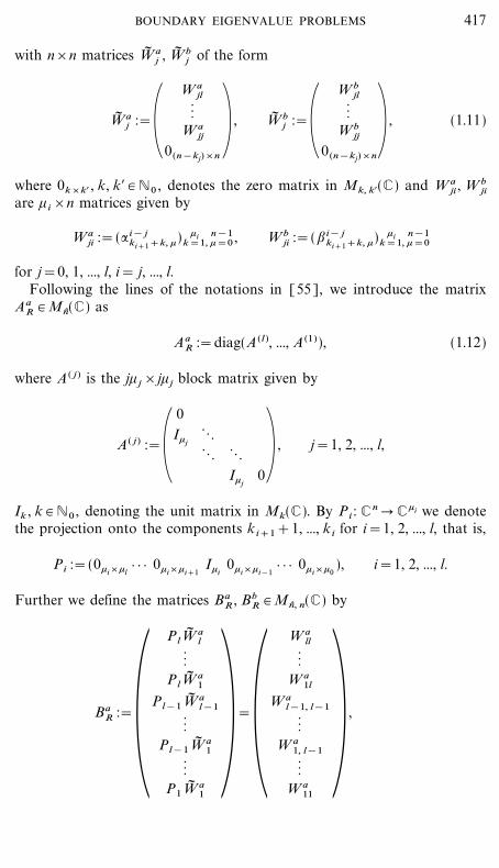
with n_n matrices W� aj , W� b
j of the form
W� aj :=\
W ajl
bW a
jj
0(n&kj)_n+ , W� b
j :=\W b
jl
bW b
jj
0(n&kj)_n+ , (1.11)
where 0k_k$ , k, k$ # N0 , denotes the zero matrix in Mk, k$(C) and W aji , W b
ji
are +i_n matrices given by
Waji :=(: i& j
ki+1+k, +) +i n&1k=1, +=0 , W b
ji :=(; i& jki+1+k, +) +i n&1
k=1, +=0
for j=0, 1, ..., l, i= j, ..., l.Following the lines of the notations in [55], we introduce the matrix
AaR # Mn(C) as
AaR :=diag(A(l ), ..., A(1)), (1.12)
where A( j ) is the j+ j _j+j block matrix given by
A( j ) :=\0I+j
. . .
. . .. . .I+j
0+ , j=1, 2, ..., l,
Ik , k # N0 , denoting the unit matrix in Mk(C). By Pi : Cn � C+i we denotethe projection onto the components ki+1+1, ..., ki for i=1, 2, ..., l, that is,
Pi :=(0+i_+l} } } 0+i_+i+1
I+i0+i_+i&1
} } } 0+i_+0), i=1, 2, ..., l.
Further we define the matrices BaR , Bb
R # M n, n(C) by
BaR :=\
PlW� al
+=\W a
ll
+ ,
b bPlW� a
1 W a1l
Pl&1 W� al&1 W a
l&1, l&1
b bPl&1W� a
1 W a1, l&1
b bP1W� a
1 W a11
417BOUNDARY EIGENVALUE PROBLEMS

File: DISTL2 382911 . By:JB . Date:12:02:01 . Time:11:11 LOP8M. V8.B. Page 01:01Codes: 2657 Signs: 856 . Length: 45 pic 0 pts, 190 mm
BbR :=\
PlW� bl
+=\W b
ll
+ , (1.13)
b bPlW� b
1 W b1l
Pl&1 W� bl&1 W b
l&1, l&1
b bPl&1W� b
1 W b1, l&1
b bP1W� b
1 W b11
and the matrix C aR # Mn, n(C) as
C aR :=(0n_+l
} } } 0n_+l
(l&1)-times
Pl* 0n_+l&1} } } 0n_+l&1
(l&2)-times
P*l&1 } } } P1*). (1.14)
By means of these matrices we introduce the boundary operators
AR : (W 12(a, b)) n � C n, AR y :=Aa
R y(a),
BR : (W 12(a, b))n � C n, BR y~ :=Ba
R y~ (a)+BbR y~ (b),
(1.15)CR : (W 1
2(a, b)) n � Cn, CR y :=C aR y(a),
DR : (W 12(a, b))n � Cn, DR y~ :=W� a
0 y~ (a)+W� b0 y~ (b),
and we define
Ja : (W 12(a, b)) n � C n, Ja y :=y(a). (1.16)
Then the linearized boundary eigenvalue problem associated with theproblem (1.1), (1.2) according to Theorem 5.1 and Corollary 6.2 of [55],is a boundary eigenvalue problem for a system of n+n first order differentialequations with *-linear boundary conditions which can be written in theform
T(*) y=(T0&*T1) y=0, y # (W 12(a, b))n+n, (1.17)
where
T(*) :=\T D(*)T R(*)+ , * # C,
418 CHRISTIANE TRETTER

File: DISTL2 382912 . By:JB . Date:12:02:01 . Time:11:11 LOP8M. V8.B. Page 01:01Codes: 2772 Signs: 743 . Length: 45 pic 0 pts, 190 mm
is given by
T D(*) y :=(T D0 &*T D
1 ) y :=y$+(A0&*A1) y, (1.18)
T R(*) y :=(T R0 &*T R
1 ) y := (W a0&*W a
1) y(a)+(W b0&*W b
1) y(b) (1.19)
for y # (W 12(a, b))n+n, that is,
T0 y=\T D0 y
T R0 y+=\ y$+A0 y
W a0 y(a)+W b
0 y(b)+ ,
(1.20)
T1 y=\T D1 y
T R1 y+=\ A1 y
W a1 y(a)+W b
1 y(b)+ .
Here the matrices A0 , A1 # Mn+n(L�(a, b)) are determined by
A0=\0 &1
0n_n +=\A� 0
000+ ,
0. . .. . . &1
f0 f1 } } } fn&1
0n_n 0n_n
A1=\0
0n_n +=\A� 1
000+ ,
. . .. . .
g0 } } } gp&1 1 0 } } } 0
0n_n 0n_n
(1.21)
and the (n+n)_(n+n) boundary matrices are of the form
W a0=\Ba
R
W� a0
AaR
C aR+ , W a
1=\00
I n
0 + ,
(1.22)
W b0=\Bb
R
W� b0
00+ , W b
1=\00
00+ ,
the entries being given by (1.12), (1.13), (1.14), and (1.11).Note that since the differential equation (1.1) is linear in *, so is T� D(*)
and hence
T D(*) y=\T� D(*) y~0
0y$+ , y=\ y~
y+ # (W 12(a, b))n+n.
419BOUNDARY EIGENVALUE PROBLEMS
File: DISTL2 382913 . By:JB . Date:12:02:01 . Time:11:11 LOP8M. V8.B. Page 01:01Codes: 2801 Signs: 1712 . Length: 45 pic 0 pts, 190 mm
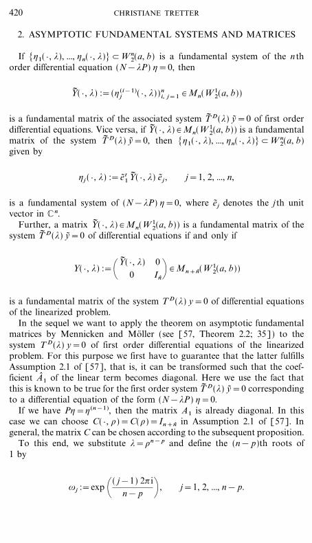
2. ASYMPTOTIC FUNDAMENTAL SYSTEMS AND MATRICES
If ['1( } , *), ..., 'n( } , *)]/W n2(a, b) is a fundamental system of the n th
order differential equation (N&*P) '=0, then
Y� ( } , *) :=(' (i&1)j ( } , *))n
i, j=1 # Mn(W 12(a, b))
is a fundamental matrix of the associated system T� D(*) y~ =0 of first orderdifferential equations. Vice versa, if Y� ( } , *) # Mn(W 1
2(a, b)) is a fundamentalmatrix of the system T� D(*) y~ =0, then ['1( } , *), ..., 'n( } , *)]/W n
2(a, b)given by
'j ( } , *) :=e~ t1Y� ( } , *) e~ j , j=1, 2, ..., n,
is a fundamental system of (N&*P) '=0, where e~ j denotes the j th unitvector in Cn.
Further, a matrix Y� ( } , *) # Mn(W 12(a, b)) is a fundamental matrix of the
system T� D(*) y~ =0 of differential equations if and only if
Y( } , *) :=\Y� ( } , *)0
0I n+ # Mn+n(W 1
2(a, b))
is a fundamental matrix of the system T D(*) y=0 of differential equationsof the linearized problem.
In the sequel we want to apply the theorem on asymptotic fundamentalmatrices by Mennicken and Mo� ller (see [57, Theorem 2.2; 35]) to thesystem T D(*) y=0 of first order differential equations of the linearizedproblem. For this purpose we first have to guarantee that the latter fulfillsAssumption 2.1 of [57], that is, it can be transformed such that the coef-ficient A� 1 of the linear term becomes diagonal. Here we use the fact thatthis is known to be true for the first order system T� D(*) y~ =0 correspondingto a differential equation of the form (N&*P) '=0.
If we have P'='(n&1), then the matrix A1 is already diagonal. In thiscase we can choose C( } , \)=C(\)=In+n in Assumption 2.1 of [57]. Ingeneral, the matrix C can be chosen according to the subsequent proposition.
To this end, we substitute *=\n& p and define the (n& p)th roots of1 by
|j :=exp \( j&1) 2? in& p + , j=1, 2, ..., n& p.
420 CHRISTIANE TRETTER
File: DISTL2 382914 . By:JB . Date:12:02:01 . Time:11:11 LOP8M. V8.B. Page 01:01Codes: 2656 Signs: 895 . Length: 45 pic 0 pts, 190 mm
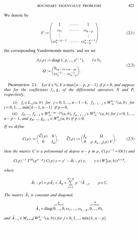
We denote by
V :=\1
|1
b|n&p&1
1
} } } } } }} } } } } }
} } } } } }
1|n&p
b|n&p&1
n&p+ (2.1)
the corresponding Vandermonde matrix, and we set
2l (\) :=diag(1, \, ..., \l&1), l # N,(2.2)
0 :=\0( p&1)_(n& p)
|&11 } } } |&1
n& p+ .
Proposition 2.1. Let k # N, k�max[n& p, p&1] if p>0, and supposethat for the coefficients f& , g& of the differential operators N and P,respectively,
(i) fj # L�(a, b) for j=0, 1, ..., n&1&k, fn&1& j # W k& j� (a, b) for
j=0, 1, ..., min[k&1, n&1] if p=0,
(ii) f0 , ..., fp&1 # W k&(n& p)� (a, b), fn&1& j # W k& j
� (a, b) for j=0, 1, ...,n& p&1, and g0 , ..., gp&1 # W k
�(a, b) if p>0.
If we define
C(\) :=\C� (\)0
0I n+ , C� (\) :=\Ip
00
\ 2n& p(\) V+ , (2.3)
then the matrix C is a polynomial of degree n& p in \, C(\)&1=O(1) and
C(\)&1 T D(\n& p) C(\) y= y$&A� ( } , \) y, y # (W 12(a, b))n+n,
where
A� ( } , \)=\A� 1+A� 0+ :n& p
j=1
\& jA� & j , \ # C.
The matrix A� 1 is constant and diagonal,
A� 1=diag(0, ..., 0
p
, |1 , ..., |n& p , 0, ..., 0
n
),
and A� & j # Mn+ n(W k& j� (a, b)) for j=0, 1, ..., min[k, n& p].
421BOUNDARY EIGENVALUE PROBLEMS

File: DISTL2 382915 . By:JB . Date:12:02:01 . Time:11:11 LOP8M. V8.B. Page 01:01Codes: 2819 Signs: 1195 . Length: 45 pic 0 pts, 190 mm
Proof. According to [35, Chap. 9, (9.12)], the differential operator T� D
fulfills Assumption 2.1 of [57]: Indeed,
C� (\)&1 T� D(\n& p) C� (\) y~ = y~ $&A�� ( } , \) y~ , y~ # (W 12(a, b))n,
where
A�� ( } , \)=\A�� 1+A�� 0+ :n& p
j=1
\& jA�� & j , \ # C,
with
A�� 1=diag(0, ..., 0
p
, |1 , ..., |n& p)
and A�� & j # Mn(W k& j� (a, b)) for j=0, 1, ..., min[k, n& p] if the coefficients
f& , g& fulfill the assumptions stated in the proposition. Obviously, thematrix C� is a polynomial of degree n& p in \. From
C� (\)&1=\Ip
0&0V &1\&1 2n& p(\&1)
V&1\&1 2n& p(\&1) +it follows that C� (\)&1= O(1). By definition of C(\),
C(\)&1 T D(\n& p) C(\) y=\C� (\)&1 T� D(\n& p) C� (\) y~0
0y$+ ,
y=\ y~y+ # (W 1
2(a, b))n+ n.
Hence if we let
A� &j=\A�� &j
00
0 n+ , j=&1, 0, ..., n&p, (2.4)
the proposition follows. K
It should be mentioned that there also exists a transformation of thesystem of differential equations T� D(\n& p) y~ =0 associated with N'=*P'and hence of T D(\n& p) y=0 given by (1.18) into a system which is notonly asymptotically but in fact linear in \ with diagonal \�linear term. Thistransformation is due to E. Wagenfu� hrer (see [58]). For estimating theGreen's function, however, it does not give more than the asymptoticdiagonalization of the *-linear coefficient used here.
422 CHRISTIANE TRETTER
File: DISTL2 382916 . By:JB . Date:12:02:01 . Time:11:11 LOP8M. V8.B. Page 01:01Codes: 2919 Signs: 1561 . Length: 45 pic 0 pts, 190 mm
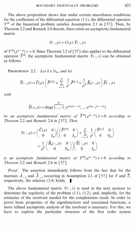
The above proposition shows that under certain smoothness conditionsfor the coefficients of the differential equation (1.1), the differential operatorT D of the linearized problem satisfies Assumption 2.1 in [57]. Then, byTheorem 2.2 and Remark 2.4 therein, there exists an asymptotic fundamentalmatrix
Y( } , \)=C(\) Y� ( } , \)
of T D(\n& p) y=0. Since Theorem 2.2 of [57] also applies to the differentialoperator T� D, the asymptotic fundamental matrix Y( } , *) can be obtainedas follows.
Proposition 2.2. Let k # N0 , and let
Y� ( } , \)=C� (\) \P� [0]+ :k
r=1
1\r P� [r]+
1\k B� k( } , \)+ E� ( } , \)
with
E� (x, \)=diag(1, ..., 1p
, e\|1(x&a), ..., e\|n&p(x&a))
be an asymptotic fundamental matrix of T� D(\n& p) y~ =0 according toTheorem 2.2 and Remark 2.4 in [57]. Then
Y( } , \)=\C� (\)0
0I n+\\
P� [0]
00I n++ :
k
r=1
1\r \P� [r]
000 n+
+1\k \B� k( } , \)
00
0 n++\E� ( } , \)
00In+
is an asymptotic fundamental matrix of T D(\n& p) y=0 according toTheorem 2.2 and Remark 2.4 in [57].
Proof. The assertion immediately follows from the fact that for thematrices A� & j and A�� & j occurring in Assumption 2.1 of [57] for T and T� ,respectively, the relation (2.4) holds. K
The above fundamental matrix Y( } , *) is used in the next sections todetermine the regularity of the problem (1.1), (1.2), and, implicitly, for theestimates of the resolvent needed for the completeness result. In order toprove basis properties of the eigenfunctions and associated functions, amore refined asymptotic analysis of the resolvent is necessary. For this, wehave to explore the particular structure of the first order system
423BOUNDARY EIGENVALUE PROBLEMS

File: DISTL2 382917 . By:JB . Date:12:02:01 . Time:11:11 LOP8M. V8.B. Page 01:01Codes: 2971 Signs: 1124 . Length: 45 pic 0 pts, 190 mm
T� D(*) y~ =0 associated with a differential equation of the form (N&*P) '=0 and of the corresponding system T D(*) y=0 of the linearized problem.
Following the lines of [35, 36], we denote by =i , =i the i th unit vectorsin C p and Cn& p, respectively. Further, let
0n& p :=diag(|1 , ..., |n& p), (2.5)
V� :=\1
|1
b| p&1
1
} } } } } }} } } } } }
} } } } } }
1|n&p
b| p&1
n&p+ , (2.6)
and let V, 2l (\) be given by (2.1), (2.2).
Theorem 2.3. Let k # N, k�max[n& p, p&1] if p>0, and supposethat
(i) fj # L�(a, b) for j=0, 1, ..., n&1&k, fn&1& j # W k& j� (a, b) for
j=0, 1, ..., min[k&1, n&1] if p=0,
(ii) f0 , ..., fp&1 # W k&(n& p)� (a, b), fn&1& j # W k& j
� (a, b) for j=0, 1, ...,n& p&1, and g0 , ..., gp&1 # W k
�(a, b) if p>0.
Then there exists a fundamental matrix Y0( } , \) of T D(\n& p) y=0 suchthat for sufficiently large \ in C,
,11( } , \) ,12( } , \) 0
Y0( } , \)=\,21( } , \) ,22( } , \) 0+ E( } , \),
0 0 In
where
E(x, \)=diag(1, ..., 1
p
, e\|1(x&a), ..., e\|n&p(x&a), 1, ..., 1
n
)
Ip 0 0
=: \ 0 E� n& p(x, \) 0+0 0 In
with the following properties:
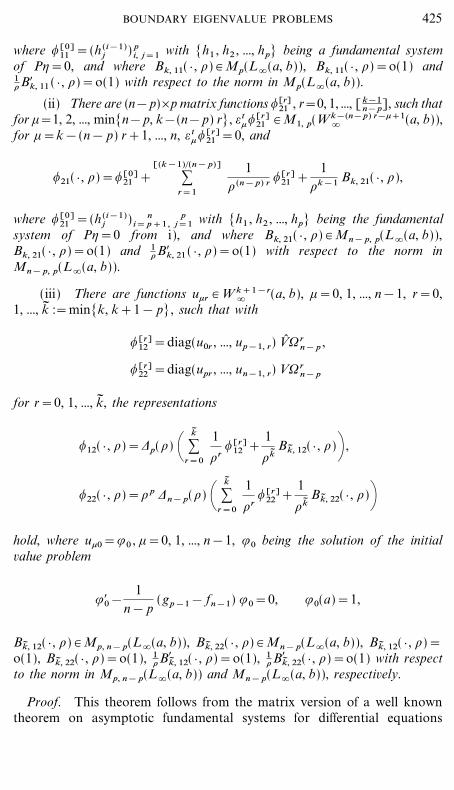
(i) There are p_p matrix functions ,[r]11 , r=0, 1, ..., [ k
n& p], suchthat for +=1, 2, ..., p, =t
+,[r]11 # M1, p(W k+ p&(n& p) r&++1
� (a, b)) and
,11( } , \)=,[0]11 + :
[k�(n& p)]
r=1
1\(n& p) r ,[r]
11 +1\k Bk, 11( } , \),
424 CHRISTIANE TRETTER
File: DISTL2 382918 . By:JB . Date:12:02:01 . Time:11:11 LOP8M. V8.B. Page 01:01Codes: 3389 Signs: 1468 . Length: 45 pic 0 pts, 190 mm
where ,[0]11 =(h (i&1)
j ) pi, j=1 with [h1 , h2 , ..., hp] being a fundamental system
of P'=0, and where Bk, 11( } , \) # Mp(L�(a, b)), Bk, 11( } , \)=o(1) and1\B$k, 11 ( } , \)=o(1) with respect to the norm in Mp(L�(a, b)).
(ii) There are (n&p)_p matrix functions ,[r]21 , r=0, 1, ..., [k&1
n&p], such thatfor +=1, 2, ..., min[n&p, k&(n&p) r], =t
+,[r]21 # M1, p(W k&(n&p) r&++1
� (a, b)),for +=k&(n& p) r+1, ..., n, = t
+,[r]21 =0, and
,21( } , \)=,[0]21 + :
[(k&1)�(n& p)]
r=1
1\ (n& p) r ,[r]
21 +1
\k&1 Bk, 21( } , \),
where ,[0]21 =(h (i&1)
j ) ni= p+1,
pj=1 with [h1 , h2 , ..., hp] being the fundamental
system of P'=0 from i), and where Bk, 21( } , \) # Mn& p, p(L�(a, b)),Bk, 21( } , \)=o(1) and 1
\B$k, 21 ( } , \)=o(1) with respect to the norm inMn& p, p(L�(a, b)).
(iii) There are functions u+r # W k+1&r� (a, b), +=0, 1, ..., n&1, r=0,
1, ..., k� :=min[k, k+1& p], such that with
,[r]12 =diag(u0r , ..., up&1, r) V� 0r
n& p ,
,[r]22 =diag(upr , ..., un&1, r) V0r
n& p
for r=0, 1, ..., k� , the representations
,12( } , \)=2p(\) \ :k�
r=0
1
\r,[r]
12 +1
\k�Bk� , 12( } , \)+ ,
,22( } , \)=\ p 2n& p(\) \ :k�
r=0
1
\r,[r]
22 +1
\k�Bk� , 22( } , \)+
hold, where u+0=.0 , +=0, 1, ..., n&1, .0 being the solution of the initialvalue problem
.$0&1
n& p(gp&1& fn&1) .0=0, .0(a)=1,
Bk� , 12( } , \) # Mp, n& p(L�(a, b)), Bk� , 22( } , \) # Mn& p(L�(a, b)), Bk� , 12( } , \)=o(1), Bk� , 22( } , \)=o(1), 1
\B$k� , 12( } , \)=o(1), 1\B$k� , 22( } , \)=o(1) with respect
to the norm in Mp, n& p(L�(a, b)) and Mn& p(L�(a, b)), respectively.
Proof. This theorem follows from the matrix version of a well knowntheorem on asymptotic fundamental systems for differential equations
425BOUNDARY EIGENVALUE PROBLEMS

File: DISTL2 382919 . By:JB . Date:12:02:01 . Time:11:11 LOP8M. V8.B. Page 01:01Codes: 2537 Signs: 1305 . Length: 45 pic 0 pts, 190 mm
N'=*P' going back to W. Eberhard and G. Freiling [15], and toR. Mennicken and M. Mo� ller [35, 36]. It follows from the respectiveTheorem 2.2 in [57] if we set
D 0 0
Y0( } , \) :=\Y� 0( } , \)0
0In+ :=Y( } , \) \ 0 \ p&10 p
n&p 0 + , (2.7)
0 0 In
where Y( } , \) is an asymptotic fundamental matrix of T D(\n& p) y=0according to Theorem 2.2 and Remark 2.4 of [57], with C(\) as inProposition 2.1 (see Proposition 2.2) and D # Mp(C) is a suitably choseninvertible matrix. A more detailed proof (for the asymptotic structure ofY� 0( } , \)) can be found in [36, Chap. VIII]. K
Sometimes the following notation is used in order to abbreviateasymptotic expansions.
Notation 2.4. Let l # N0 , and let g be a function on C with values in aBanach space X. If g has an asymptotic representation
g(\)= f (\)+O \ 1\l+1+ , f (\)= f0+
f1
\+ } } } +
fl
\l ,
with f0 , f1 , ..., fl # X for \ # C, \ � �, with respect to the norm in X, thenwe write
g(\)=[ f (\)]l .
We omit the index l if l=0. If precise information on f (\) is not necessary,we will write [V (\)] l , [V ( } , \)] or [V (x, \)] l , respectively, if we want toindicate that x, for example, is the independent variable in the case that Xis a function space.
Corollary 2.5. Let k # N, k�max[n& p+1, p&1] if p>0. Then,under the further assumptions of Theorem 2.3,
,� 11( } , \) ,� 12( } , \) 0
Y $0( } , \)=\,� 21( } , \) ,� 22( } , \) 0 + E( } , \),
0 0 0 n
426 CHRISTIANE TRETTER
File: DISTL2 382920 . By:JB . Date:12:02:01 . Time:11:11 LOP8M. V8.B. Page 01:01Codes: 3340 Signs: 1450 . Length: 45 pic 0 pts, 190 mm
where
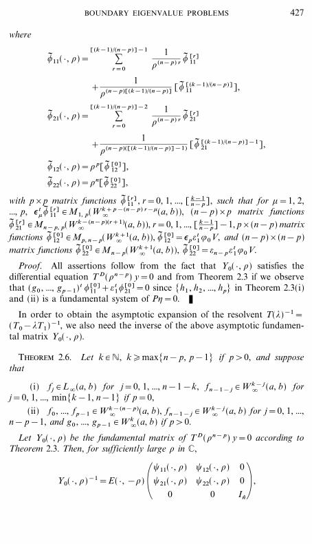
,� 11( } , \)= :[(k&1)�(n& p)]&1
r=0
1\ (n& p) r ,� [r]
11
+1
\(n& p)[(k&1)�(n& p)] [,� [(k&1)�(n& p)]11 ],
,� 21( } , \)= :[(k&1)�(n& p)]&2
r=0
1\ (n& p) r ,� [r]
21
+1
\(n& p)([(k&1)�(n& p)]&1) [,� [(k&1)�(n& p)]&121 ],
,� 12( } , \)=\ p[,� [0]12 ],
,� 22( } , \)=\n[,� [0]22 ],
with p_p matrix functions ,� [r]11 , r=0, 1, ..., [ k&1
n& p], such that for +=1, 2,..., p, = t
+,� [r]11 # M1, p(W k+ p&(n& p) r&+
� (a, b)), (n& p)_p matrix functions,� [r]
21 # Mn& p, p(W k&(n& p)(r+1)� (a, b)), r=0, 1, ..., [ k&1
n& p]&1, p_(n& p) matrixfunctions ,� [0]
12 # Mp, n& p(W k+1� (a, b)), ,� [0]
12 ==p=t1.0V, and (n& p)_(n& p)
matrix functions ,� [0]22 # Mn& p(W k+1
� (a, b)), ,� [0]22 ==n& p= t
1.0 V.
Proof. All assertions follow from the fact that Y0( } , \) satisfies thedifferential equation T D(\n& p) y=0 and from Theorem 2.3 if we observethat (g0 , ..., gp&1)t ,[0]
11 += t1,[0]
21 =0 since [h1 , h2 , ..., hp] in Theorem 2.3(i)and (ii) is a fundamental system of P'=0. K
In order to obtain the asymptotic expansion of the resolvent T(*)&1=(T0&*T1)&1, we also need the inverse of the above asymptotic fundamen-tal matrix Y0( } , \).
Theorem 2.6. Let k # N, k�max[n& p, p&1] if p>0, and supposethat
(i) fj # L�(a, b) for j=0, 1, ..., n&1&k, fn&1& j # W k& j� (a, b) for
j=0, 1, ..., min[k&1, n&1] if p=0,
(ii) f0 , ..., fp&1 # W k&(n& p)� (a, b), fn&1& j # W k& j
� (a, b) for j=0, 1, ...,n& p&1, and g0 , ..., gp&1 # W k
�(a, b) if p>0.
Let Y0( } , \) be the fundamental matrix of T D(\n& p) y=0 according toTheorem 2.3. Then, for sufficiently large \ in C,
�11( } , \) �12( } , \) 0
Y0( } , \)&1=E( } , &\) \�21( } , \) �22( } , \) 0+ ,
0 0 I n
427BOUNDARY EIGENVALUE PROBLEMS

File: DISTL2 382921 . By:JB . Date:12:02:01 . Time:11:21 LOP8M. V8.B. Page 01:01Codes: 2784 Signs: 1142 . Length: 45 pic 0 pts, 190 mm
where
E(x, \)=diag(1, ..., 1
p
, e\|1(x&a), ..., e\|n&p(x&a), 1, ..., 1
n
)
with the following properties:
(i) There are matrix functions �[r]11 # Mp(W k+1&(n& p) r
� ), r=0, 1, ...,[ k
n& p], such that
�11( } , \)= :[k�(n& p)]
r=0
1\(n& p) r �[r]
11 +1\k Dk, 11( } , \),
where Dk, 11( } , \) # Mp(L�(a, b)) such that Dk, 11( } , \) = o(1) and1\ D$k, 11 ( } , \)=o(1) with respect to the norm in Mp(L�(a, b)).
(ii) There are p_(n& p) matrix functions �[r]12 , r=0, 1, ..., [ k
n& p],such that for +=1, 2, ..., n& p, �[r]
12 =+ # M1, p(W k&(n& p)(r+1)+++1� (a, b))
and
�12( } , \)=1
\n& p :[k�(n& p)]
r=0
1\ (n& p) r �[r]
12 +1
\k+1 Dk, 12( } , \) 2n& p(\)&1,
where
�[0]12 =n& p=&,[0]
11&1=p ,
and Dk, 12( } , \) # Mp, n& p(L�(a, b)) such that Dk, 12( } , \) = o(1),1\ D$k, 12 ( } , \)=o(1) with respect to the norm in Mp, n& p(L�(a, b)).
(iii) There are matrix functions �[r]21 # Mn& p, p(W k+1&r
� (a, b)),r=0, 1, ..., k, such that
�21( } , \)=1
\ p \ :k
r=0
1\r �[r]
21 +1\k Dk, 21( } , \)+ ,
where Dk, 21( } , \) # Mn& p, p(L�(a, b)) such that Dk, 21( } , \)=o(1) and1\ D$k, 21 ( } , \)=o(1) with respect to the norm in Mn& p, p(L�(a, b)).
(iv) There are matrix functions �[r]22 # Mn& p(W k+1&r
� (a, b)), r=0, 1,..., k, such that
�22( } , \)=1
\ p \ :k
r=0
1\r �[r]
22 +1\k Dk, 22( } , \)+ 2n& p(\)&1,
where
�[0]22 =,[0]&1
22 =.&10 |&p
n& pV &1,
428 CHRISTIANE TRETTER
File: DISTL2 382922 . By:JB . Date:12:02:01 . Time:11:21 LOP8M. V8.B. Page 01:01Codes: 2863 Signs: 1277 . Length: 45 pic 0 pts, 190 mm
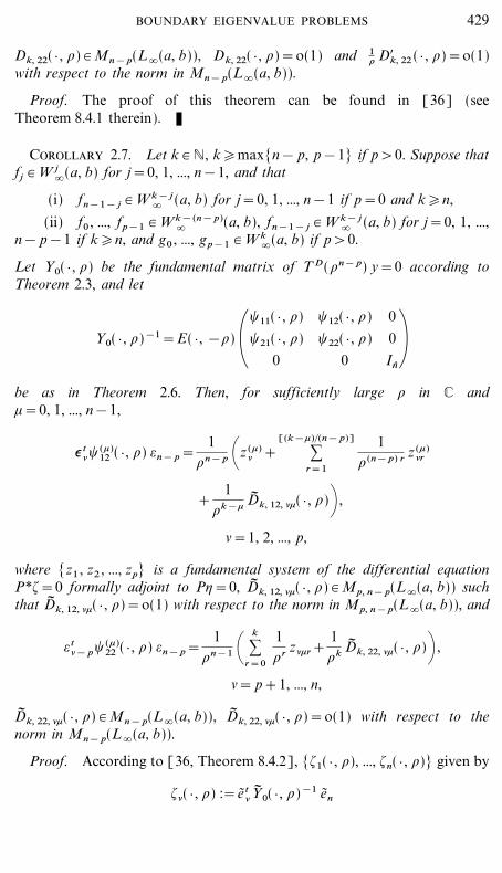
Dk, 22( } , \) # Mn& p(L�(a, b)), Dk, 22( } , \)=o(1) and 1\ D$k, 22 ( } , \)=o(1)
with respect to the norm in Mn& p(L�(a, b)).
Proof. The proof of this theorem can be found in [36] (seeTheorem 8.4.1 therein). K
Corollary 2.7. Let k # N, k�max[n& p, p&1] if p>0. Suppose thatfj # W j
�(a, b) for j=0, 1, ..., n&1, and that
(i) fn&1& j # W k& j� (a, b) for j=0, 1, ..., n&1 if p=0 and k�n,
(ii) f0 , ..., fp&1 # W k&(n& p)� (a, b), fn&1& j # W k& j
� (a, b) for j=0, 1, ...,n& p&1 if k�n, and g0 , ..., gp&1 # W k
�(a, b) if p>0.
Let Y0( } , \) be the fundamental matrix of T D(\n& p) y=0 according toTheorem 2.3, and let
�11( } , \) �12( } , \) 0
Y0( } , \)&1=E( } , &\) \�21( } , \) �22( } , \) 0+0 0 In
be as in Theorem 2.6. Then, for sufficiently large \ in C and+=0, 1, ..., n&1,
= t&� (+)
12 ( } , \) =n& p=1
\n& p \z (+)& + :
[(k&+)�(n& p)]
r=1
1\(n& p) r z (+)
&r
+1
\k&+ D� k, 12, &+( } , \)+ ,
&=1, 2, ..., p,
where [z1 , z2 , ..., zp] is a fundamental system of the differential equationP*`=0 formally adjoint to P'=0, D� k, 12, &+( } , \) # Mp, n& p(L�(a, b)) suchthat D� k, 12, &+( } , \)=o(1) with respect to the norm in Mp, n& p(L�(a, b)), and
=t&& p� (+)
22 ( } , \) =n& p=1
\n&1 \ :k
r=0
1\r z&+r+
1\k D� k, 22, &+( } , \)+ ,
&= p+1, ..., n,
D� k, 22, &+( } , \) # Mn& p(L�(a, b)), D� k, 22, &+( } , \)=o(1) with respect to thenorm in Mn& p(L�(a, b)).
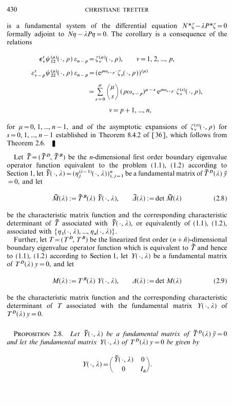
Proof. According to [36, Theorem 8.4.2], [`1( } , \), ..., `n( } , \)] given by
`&( } , \) :=e~ t&Y� 0( } , \)&1 e~ n
429BOUNDARY EIGENVALUE PROBLEMS
File: DISTL2 382923 . By:JB . Date:12:02:01 . Time:11:21 LOP8M. V8.B. Page 01:01Codes: 2818 Signs: 1483 . Length: 45 pic 0 pts, 190 mm
is a fundamental system of the differential equation N*`&*P*`=0formally adjoint to N'&*P'=0. The corollary is a consequence of therelations
=t&� (+)
12 ( } , \) =n& p=` (+)& ( } , \), &=1, 2, ..., p,
=t&& p� (+)
22 ( } , \) =n& p=(e\|&&p } `&( } , \)) (+)
= :+
s=0\+
s+ (\|&& p)+&s e\|&&p } ` (s)& ( } , \),
&= p+1, ..., n,
for +=0, 1, ..., n&1, and of the asymptotic expansions of `(s)& ( } , \) for
s=0, 1, ..., n&1 established in Theorem 8.4.2 of [36], which follows fromTheorem 2.6. K
Let T� =(T� D, T� R) be the n-dimensional first order boundary eigenvalueoperator function equivalent to the problem (1.1), (1.2) according toSection 1, let Y� ( } , *)=(' (i&1)
j ( } , *))ni, j=1 be a fundamental matrix of T� D(*) y~
=0, and let
M� (*) :=T� R(*) Y� ( } , *), 2� (*) :=det M� (*) (2.8)
be the characteristic matrix function and the corresponding characteristicdeterminant of T� associated with Y� ( } , *), or equivalently of (1.1), (1.2),associated with ['1( } , *), ..., 'n( } , *)].
Further, let T=(T D, T R) be the linearized first order (n+n)-dimensionalboundary eigenvalue operator function which is equivalent to T� and henceto (1.1), (1.2) according to Section 1, let Y( } , *) be a fundamental matrixof T D(*) y=0, and let
M(*) :=T R(*) Y( } , *), 2(*) :=det M(*) (2.9)
be the characteristic matrix function and the corresponding characteristicdeterminant of T associated with the fundamental matrix Y( } , *) ofT D(*) y=0.
Proposition 2.8. Let Y� ( } , *) be a fundamental matrix of T� D(*) y~ =0and let the fundamental matrix Y( } , *) of T D(*) y=0 be given by
Y( } , *)=\Y� ( } , *)0
0In+ .
430 CHRISTIANE TRETTER
File: DISTL2 382924 . By:JB . Date:12:02:01 . Time:11:21 LOP8M. V8.B. Page 01:01Codes: 2838 Signs: 1516 . Length: 45 pic 0 pts, 190 mm
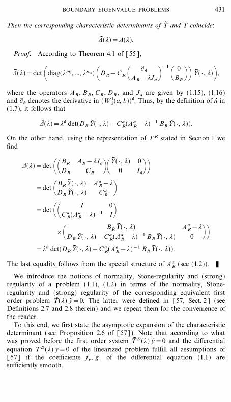
Then the corresponding characteristic determinants of T� and T coincide:
2� (*)=2(*).
Proof. According to Theorem 4.1 of [55],
2� (*)=det \diag(*m1, ..., *mn) \DR&CR \ �n
AR&*Ja+&1
\ 0BR++ Y� ( } , *)+ ,
where the operators AR , BR , CR , DR , and Ja are given by (1.15), (1.16)and �n denotes the derivative in (W 1
2(a, b)) n. Thus, by the definition of n in(1.7), it follows that
2� (*)=*n det(DR Y� ( } , *)&C aR(Aa
R&*)&1 BR Y� ( } , *)).
On the other hand, using the representation of T R stated in Section 1 wefind
2(*)=det \\BR
DR
AR&*Ja
CR +\Y� ( } , *)0
0I n++
=det \BRY� ( } , *)DR Y� ( } , *)
AaR&*C a
R +=det \\ I
C aR(Aa
R&*)&1
0I+
_\ BRY� ( } , *)DRY� ( } , *)&C a
R(AaR&*)&1 BR Y� ( } , *)
AaR&*0 ++
=*n det(DR Y� ( } , *)&C aR(Aa
R&*)&1 BR Y� ( } , *)).
The last equality follows from the special structure of AaR (see (1.2)). K
We introduce the notions of normality, Stone-regularity and (strong)regularity of a problem (1.1), (1.2) in terms of the normality, Stone-regularity and (strong) regularity of the corresponding equivalent firstorder problem T� (*) y~ =0. The latter were defined in [57, Sect. 2] (seeDefinitions 2.7 and 2.8 therein) and we repeat them for the convenience ofthe reader.
To this end, we first state the asymptotic expansion of the characteristicdeterminant (see Proposition 2.6 of [57]). Note that according to whatwas proved before the first order system T� D(*) y~ =0 and the differentialequation T D(*) y=0 of the linearized problem fulfill all assumptions of[57] if the coefficients f& , g& of the differential equation (1.1) aresufficiently smooth.
431BOUNDARY EIGENVALUE PROBLEMS

File: DISTL2 382925 . By:JB . Date:12:02:01 . Time:11:21 LOP8M. V8.B. Page 01:01Codes: 2745 Signs: 1182 . Length: 45 pic 0 pts, 190 mm
Proposition 2.9. Let k # N0 , and let
Y� ( } , \)=C� (\) \P� [0]+ :k
r=1
1\r P� [r]+
1\k B� k( } , \)+ E� ( } , \),
\n& p=*, be an asymptotic fundamental matrix of T� D(\n& p) y~ =0 accordingto Theorem 2.2 and Remark 2.4 in [57], where C� (\) is chosen according toAssumption 2.1 of [57],
E� ( } , \)=diag(E0( } , \), E1( } , \), ..., En( } , \)),
E&(x, \)=exp \\ |x
ar~ &(!) d!+ ,
where r~ & , &=1, 2, ..., n, are the diagonal elements of A� 1 or A�� 1 , respectively.Then, for sufficiently large \ # C, the characteristic determinant 2� of (1.1),(1.2) has an asymptotic expansion
2� (\)=\q~ 0 :c # E
[bc(\)]k&1 e\c,
where q~ 0 is defined as
q~ 0 :=q~ 1+q~ 2+ } } } +q~ n (2.10)
with
q~ i :=max[deg(e~ ti W� a(\n& p) C� (\)), deg(e~ t
i W� b(\n& p) C� (\))], (2.11)
i=1, 2, ..., n.
Here e~ i denotes the ith unit vector in Cn, E is the set
E={ :n
&=1
R� &(x(&)) : x(&) # [a, b], &=1, 2, ..., n= ,
and
bc(\)=bc0+bc1
\+ } } } +
bc, k&1
\k&1
are polynomials of order k&1 in \&1.
Definition 2.10. Let k # N0 and Y� ( } , \) be a fundamental matrix ofT� D(\n& p) y=0 as in Proposition 2.9 above. We denote by M the smallestconvex polygon containing all points c # E. For r # [0, 1, ..., k&1] wedenote by Mr the smallest convex polygon containing all points c # E forwhich bcs {0 for some s # [0, 1, ..., r]. Obviously, Mr&1 /Mr /M.
432 CHRISTIANE TRETTER

File: DISTL2 382926 . By:JB . Date:12:02:01 . Time:11:21 LOP8M. V8.B. Page 01:01Codes: 3012 Signs: 2119 . Length: 45 pic 0 pts, 190 mm
The problem T� (*) y~ =0 is called normal if there exists a number}0 # [0, 1, ..., k&1] with the following properties:
(i) The polygon M}0has at least 2 points of tangency with M.
(ii) The perpendiculars constructed from a certain fixed interiorpoint of M to the sides of M on which the points of tangency lie divide thecomplex plane into sectors of angle less than ?.
If M is a segment, the problem is called normal if there exists a}0 # [0, 1, ..., k&1] such that
(iii) M}0=M.
If }0 is the least number such that (i), (ii), and (iii), respectively, hold, thenthe problem T� (*) y~ =0 is said to be normal of order }0 .
The problem T� (*) y~ =0 is called Stone-regular if M}0=M for some num-
ber }0 # [0, 1, ..., k&1]. If }0 is the smallest number with this property,then it is called Stone-regular of order }0 . A Stone-regular problemT� (*) y~ =0 of order 0 is called regular. A regular problem T� (*) y~ =0 iscalled strongly regular if asymptotically the zeros of the characteristic deter-minant 2� are simple and differ from one another by some positive constant$>0. Note that any Stone-regular problem of order }0 is normal oforder }0 .
Definition 2.11. Let }0 # N. The problem (1.1), (1.2) is called normalof order }0 (Stone-regular of order }0 , (strongly) regular) if the associatedfirst order problem T� (*) y~ =0 is normal of order }0 (Stone-regular of order}0 , (strongly) regular).
In order to relate the various notions of regularity of the problem (1.1),(1.2) to those of the corresponding linearized problem (1.17) (which aredefined according to [57], analogously to Definition 2.10), we use therelation of the respective asymptotic fundamental matrices establishedpreviously.
Theorem 2.12. If the problem (1.1), (1.2) is normal of order }0
(Stone-regular of order }0 , (strongly) regular), then the associated linearizedproblem T(*) y=0 is normal of order }0 (Stone-regular of order }0 ,(strongly) regular).
Proof. By Proposition 2.2 the asymptotic fundamental matrices Y� ( } , *)of T� D(\n& p) y~ =0 and Y( } , *) of T D(\n& p) y=0 according toTheorem 2.2 and Remark 2.4 of [57], are related by
Y( } , *)=\Y� ( } , *)0
0In+ .
433BOUNDARY EIGENVALUE PROBLEMS
File: DISTL2 382927 . By:JB . Date:12:02:01 . Time:11:21 LOP8M. V8.B. Page 01:01Codes: 2319 Signs: 1289 . Length: 45 pic 0 pts, 190 mm
By Proposition 2.8, the asymptotic expansions of 2� (\) and 2(\)coincide. K
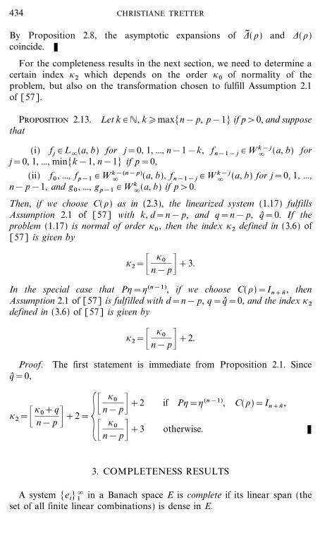
For the completeness results in the next section, we need to determine acertain index }2 which depends on the order }0 of normality of theproblem, but also on the transformation chosen to fulfill Assumption 2.1of [57].
Proposition 2.13. Let k # N, k�max[n& p, p&1] if p>0, and supposethat
(i) fj # L�(a, b) for j=0, 1, ..., n&1&k, fn&1& j # W k& j� (a, b) for
j=0, 1, ..., min[k&1, n&1] if p=0,
(ii) f0 , ..., fp&1 # W k&(n& p)� (a, b), fn&1& j # W k& j
� (a, b) for j=0, 1, ...,n& p&1, and g0 , ..., gp&1 # W k
�(a, b) if p>0.
Then, if we choose C(\) as in (2.3), the linearized system (1.17) fulfillsAssumption 2.1 of [57] with k, d=n& p, and q=n& p, q=0. If theproblem (1.17) is normal of order }0 , then the index }2 defined in (3.6) of[57] is given by
}2=_ }0
n& p&+3.
In the special case that P'='(n&1), if we choose C(\)=In+ n , thenAssumption 2.1 of [57] is fulfilled with d=n& p, q=q=0, and the index }2
defined in (3.6) of [57] is given by
}2=_ }0
n& p&+2.
Proof. The first statement is immediate from Proposition 2.1. Sinceq=0,
}2=_}0+qn& p &+2={_
}0
n& p&+2 if P'=' (n&1), C(\)=In+n ,
_ }0
n& p&+3 otherwise. K
3. COMPLETENESS RESULTS
A system [ei]�1 in a Banach space E is complete if its linear span (the
set of all finite linear combinations) is dense in E.
434 CHRISTIANE TRETTER
File: DISTL2 382928 . By:JB . Date:12:02:01 . Time:11:21 LOP8M. V8.B. Page 01:01Codes: 2897 Signs: 1485 . Length: 45 pic 0 pts, 190 mm
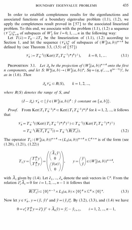
In order to establish completeness results for the eigenfunctions andassociated functions of a boundary eigenvalue problem (1.1), (1.2), weapply the completeness result proved in [57] to the associated linearizedproblem. To this end, we associate with the problem (1.1), (1.2) a sequence(V l
k)�k=0 of subspaces of W l
2 for l=0, 1, ..., n in the following way:Let T(*)=T0&*T1 be the linearization of (1.1), (1.2) according to
Section 1, and let the sequence (Vk)�0 of subspaces of (W 1
2(a, b))n+n bedefined by (see Theorem 3.3, (3.5) of [57])
Vk :=T &10 ((Ker((T1T &1
0 )*)k)=), k=0, 1, ... . (3.1)
Proposition 3.1. Let Qn be the projection of (W 12(a, b))n+n onto the first
n components, and let S: W n2(a, b) � (W 1
2(a, b))n, S'=(', '$, ..., '(n&1))t, beas in (1.6). Then
QnVk /R(S), k=1, 2, ...,
where R(S) denotes the range of S, and
(I&Qn) Vk /[ y # (W 12(a, b)) n : y constant on [a, b]].
Proof. From Ker(T1 T &10 )*/Ker((T1T &1
0 )*)k for k=1, 2, ..., it followsthat
Vk=T &10 ((Ker((T1T &1
0 )*)k)=)/T &10 ((Ker(T1 T &1
0 )*)=)
=T &10 (R(T1 T &1
0 ))=T &10 (R(T1)). (3.2)
The operator T1 : (W 12(a, b))n+n � (L2(a, b))n+n_Cn+n is of the form (see
(1.20), (1.21), (1.22))
T1 y=\T D1 y
T R1 y+=\\
A� 1 y~0 +
\y(a)0 ++ , y=\y~
y+ # (W 12(a, b))n+n,
with A� 1 given by (1.4). Let e~ 1 , ..., e~ n denote the unit vectors in Cn. From therelation e~ t
i A� 1=0 for i=1, 2, ..., n&1 it follows that
R(T1)/[0]n&1_L2(a, b)_[0] n_C n_[0]n. (3.3)
Now let y # Vk , y=( y~ , y) t and y~ =( y~ i)n1 . By (3.2), (3.3), and (1.4) we have
0=eti T D
0 y=e~ ti( y~ $+A� 0 y~ )= y~ i$& y~ i+1 , i=1, 2, ..., n&1,
435BOUNDARY EIGENVALUE PROBLEMS

File: DISTL2 382929 . By:JB . Date:12:02:01 . Time:11:21 LOP8M. V8.B. Page 01:01Codes: 3002 Signs: 1594 . Length: 45 pic 0 pts, 190 mm
where e1 , ..., en+n denote the unit vectors in Cn+ n. Hence y~ i= y~ (i&1)1 for
i=1, 2, ..., n which implies y1 # W n2(a, b) and Qn y= y~ =( y (i&1)
1 )n1=Sy1 #
R(S). Further, (I&Qn) y= y and, again by (3.2) and (3.3), y$=0. K
Definition 3.2. For l=0, 1, ..., n, we define a sequence (V lk)�
k=0 ofsubspaces of the Sobolev space W l
2(a, b) by
V lk :=S &1(QnVk) & }&2, l, k=0, 1, ..., (3.4)
where the closure is taken with respect to the norm & }&2, l in W l2(a, b).
According to the foregoing proposition, the subspaces V lk /W l
2(a, b)are well-defined, they are closed by definition and have the followingproperties:
Proposition 3.3. For k=0, 1, ..., we have
(i) Vnk=S &1(QnVk),
(ii) Vnk /Vn&1
k / } } } /V0k ,
(iii) V lk /[' # W l
2(a, b) : U 0j (')=0, mj=0, ord U j�l&1],
l=0, 1, ..., n.
The last statement implies that the functions belonging to the space V lk
satisfy the *-independent boundary conditions (1.2) of order �l&1.
Proof. Let k # [0, 1, ...].
(i) The subspace Vk /(W 12(a, b))n+n is closed by definition (see
(3.1)), since (Ker((T1T &10 )*)k)= is closed and T &1
0 is continuous. Moreover,the operators Qn and S &1: R(S) � W n
2(a, b) are continuous, and henceS&1(QnVk) is closed in W n
2(a, b).
(ii) The statement follows from the fact that the norm & }&2, l isstronger than the norm & }&2, m whenever l�m.
(iii) Let l # [0, 1, ..., n]. It is sufficient to prove that
S&1(QnVk)/[' # W l2(a, b) : U 0
j (')=0, m j=0].
Let ' # S &1(QnVk), '=S &1Qn y with y # Vk . Then we have y=( y~ , y)t withy~ =('(i&1))n
i=1 , and, by (3.2) and (3.3),
e ti T R
0 y=0, i=n+1, ..., n+n,
where T R0 is given by T R(*)=: T R
0 &*T R1 . By the representation of T R (see
(1.19), (1.22)), this implies
W� a0 y~ (a)+W� b
0 y~ (b)+C aR y(a)=0.
436 CHRISTIANE TRETTER

File: DISTL2 382930 . By:JB . Date:12:02:01 . Time:11:21 LOP8M. V8.B. Page 01:01Codes: 3182 Signs: 1852 . Length: 45 pic 0 pts, 190 mm
The last +0 rows of C aR are equal to 0 by definition (see (1.14)), the last +0
rows of W� a0 and W� b
0 are given by W a00=(:0
n&+0+k, + ) +0k=1,
n&1+=0 and W b
00=(;0
n&+0+k, + ) +0k=1,
n&1+=0 , respectively (see (1.11)). Consequently,
(:0n&+0+k, + ) +0
k=1,n&1+=0 ('(+)(a))n&1
+=0+(;0n&+0+k, +) +0
k=1,n&1+=0 ('(+)(b))n&1
+=0=0,
which is equivalent to
Uj (', *)=U 0j (')=0, j=n&+0+1, ..., n.
By definition, +0 is the number of boundary conditions (1.2) not dependingon *. Because of m1�m2� } } } �mn , the last +0 boundary conditions arejust the *-independent boundary conditions. K
Proposition 3.4. If ['s&] is a canonical system of eigenfunctions and
associated functions of the problem (1.1), (1.2), then ['s&]/V l
k for l=0, 1,..., n and k=0, 1, ... .
Proof. Let k # [0, 1, ...], and let ['s&] be a canonical system of eigenfunc-
tions and associated functions of (1.1), (1.2). According to Proposition 3.3(i)and (ii), it is sufficient to prove ['s
&]/Vnk=S&1(QnVk). By Proposition 6.4
and Proposition 3.3 of [55], there exists a canonical system [ ys&] of eigen-
functions and associated functions of the corresponding linearized problemsuch that Qn ys
&=S's&. As ys
& # Vk by Theorem 3.3 of [57], the assertionfollows. K
The main result of this section is the following completeness result:
Theorem 3.5. Let k # N, k�max[n& p, p&1] if p>0, and supposethat for the coefficients f& , g& of the differential operators N and P,respectively,
(i) fj # L�(a, b) for j=0, 1, ..., n&1&k, fn&1& j # W k& j� (a, b) for
j=0, 1, ..., min[k&1, n&1] if p=0,
(ii) f0 , ..., fp&1 # W k&(n& p)� (a, b), fn&1& j # W k& j
� (a, b) for j=0, 1, ...,n& p&1, and g0 , ..., gp&1 # W k
�(a, b) if p>0.
Let the problem (1.1), (1.2) be non-degenerate, and let ['s&] be a corresponding
canonical system of eigenfunctions and associated functions. Assume that(1.1), (1.2) is normal of order }0 , and set
}2={_}0
n& p&+2 if P'='(n&1) and C(\)=In+n ,
_ }0
n& p&+3 otherwise.(3.5)
437BOUNDARY EIGENVALUE PROBLEMS

File: DISTL2 382931 . By:JB . Date:12:02:01 . Time:11:21 LOP8M. V8.B. Page 01:01Codes: 3210 Signs: 1684 . Length: 45 pic 0 pts, 190 mm
Then the sequence (V lk)�
k=0 of subspaces of W l2 , l=0, 1, ..., n, becomes
stationary at }2 ,
V lk=V l
}2, k�}2 ,
and the system ['s&] is complete in V l
}2for l=0, 1, ..., n.
Proof. If the problem (1.1), (1.2) is normal of order }0 , then so is thelinearized problem by Theorem 2.12. The first statement is immediate fromthe definition of V l
k and from Theorem 3.3 of [57]. For the second assertionit is sufficient to prove that ['s
&] is complete in Vn}2
. According to Proposition6.4 and Proposition 3.3 of [56], the system [ ys
&]/(W 12(a, b))n+n given by
ys&=\
y~ s&
+ ,& :
s
t=0\\ �n
AR&*&Ja+&1
\ 0Ja++
s&t
\ �n
AR&*& Ja +&1
\ 0BR+ y~ t
&
where y~ s&=S's
&=(' s (i&1)& )n
i=1 , is a system of eigenfunctions and associatedfunctions of the linearized problem T(*) y=0 corresponding to (1.1), (1.2)(�n denotes the derivative in (W 1
2(a, b))n). Hence [ y s&] is complete in V}2
by Theorem 3.3 of [57]. As Qn and S &1: R(S) � W n2(a, b) are continuous
and 's&=S &1Qn ys
& , it follows that ['s&] is complete in S &1(QnV}2
)=Vn
}2. K
4. MINIMALITY RESULTS
A system [ei]�1 in a Banach space E is called minimal if there exists a
system [ f j]�1 in E$ which is biorthogonal to [e i]�
1 , i.e.,
fj (ei)=$ij , i, j=1, 2, ... .
The system [ei]�1 is called minimal with defect m, m # N0 , if there exist m
elements ei1, ..., eim
/[ei]�1 such that [ei]�
1 "[ei1, ..., eim
] is minimal and
span([ei]�1 "[ei1
, ..., eim])=span[ei]�
1 .
The number m is called the defect of minimality.By means of the minimality results for first order systems established in
[57], applied to the linearized problem (1.17), we are able to establish atheorem on the minimality of the eigenfunctions and associated functionsof a problem (1.1), (1.2) in the Sobolev spaces W l
2(a, b) of order l�p.
438 CHRISTIANE TRETTER

File: DISTL2 382932 . By:JB . Date:12:02:01 . Time:11:21 LOP8M. V8.B. Page 01:01Codes: 3333 Signs: 1863 . Length: 45 pic 0 pts, 190 mm
Theorem 4.1. Let ['s&]/W n
2(a, b) be a canonical system of eigenfunc-tions and associated functions of a non-degenerate problem (1.1), (1.2).Let T(*)=T0&*T1 be the linearization of (1.1), (1.2). Let [ ys
&]/(W 1
2(a, b))n+n and [v t+ ]/(L2(a, b))n+n_C n+n be canonical systems of
eigenfunctions and associated functions of T and T*, respectively, and defineV :=span[ ys
&], W :=span[v t+ ]. Denote by Q the orthogonal projection of
(L2(a, b))n+n_C n+n onto C n+n and set
m0 :=codimQW(QW & Q(T1V)=). (4.1)
Then m0�n, the system [P's&] is minimal with defect m0 in L2(a, b), and the
system ['s&] is minimal with defect �m0 in W l
2(a, b) for l�p.
Proof. That m0�n follows from m0�codimC n+n Q(T1 V)= and fromR(T1)/(L2(a, b))n+ n_C n_[0]n which implies [0] n_Cn/Q(T1V)=.Further, let P :=I&Q be the orthogonal projection of (L2(a, b))n+n_C n+n
onto (L2(a, b))n+n. By Proposition 3.8 of [57], the system
[PT1 y s&]={\A� 1 y~ s
&
0 += ,
where y~ s&=('s
&(i&1))n
i=1 , is minimal with defect m0 in (L2(a, b))n+n. Then,clearly, [A� 1 y~ s
&] is minimal with defect m0 in (L2(a, b))n. By (1.4),
A� 1 y~ s&=\
0
g0 } } } gp&1
. . .
1
. . .0 } } } 0+\
' s&
' s&$b
's(n&1)&
+=\0b0
P's&+ ,
where P is the differential operator on the right hand side of (1.1). Thus[P's
&] is minimal with defect m0 in L2(a, b). This proves the first statement.The second assertion follows from Remark 2.9(i) of [56], and from the
fact that for l�p, the operator P: W l2(a, b) � W l& p
2 (a, b) is bounded. K
Remark 4.2. If the coefficients of (1.1) are sufficiently smooth and theproblem (1.1), (1.2) is normal of order }0 , then V=V}2
, W=W}2are the
spaces associated with the linearization T and its adjoint T* according toTheorem 3.3 and Theorem 3.4 of [57], respectively.
Corollary 4.3. Let the coefficients of (1.1) fulfill the assumptions ofTheorem 3.5, let the problem (1.1), (1.2) be normal of order }0 , and letV l
}2/W l
2 be as in Definition 3.2.
439BOUNDARY EIGENVALUE PROBLEMS

File: DISTL2 382933 . By:JB . Date:12:02:01 . Time:11:21 LOP8M. V8.B. Page 01:01Codes: 2915 Signs: 2176 . Length: 45 pic 0 pts, 190 mm
If P: V p}2
� L2(a, b) is invertible, then [' s&] is minimal with defect m0 in
W l2(a, b) for l�p. In particular, if there are at least p *-independent boundary
conditions of order �p&1, then ['s&] is minimal with defect m0 in W l
2(a, b)for l�p.
Proof. By Proposition 3.4, ['s&]/V p
}2. Since P is a Fredholm operator,
the assumption implies that the inverse P&1: R(P) � V p}2
is bounded. Thenthe first assertion follows from Remark 2.9(i) of [56]. The secondstatement follows from the first one as ' # V p
}2implies that ' fulfills all
*-independent boundary conditions of order �p&1 by Proposition 3.3. K
5. RIESZ BASIS PROPERTIES
A system [ei]�1 in a Banach space E is called a basis if any element x # E
has a unique representation
x= :�
i=1
ci ei (5.1)
with respect to the norm of E. The basis [ei]�1 is called unconditional if the
series in (5.1) converges unconditionally. If (5.1) converges (uncondi-tionally) in E only after putting some of its terms in parentheses thearrangement of which does not depend on x, then [ei]�
1 is called a basiswith parentheses (an unconditional basis with parentheses) in E. Anunconditional basis (with parentheses) in a Hilbert space is a Riesz basis(with parentheses) up to normalization. If the system [ei]�
1 is only mini-mal with defect m in E, then [ei]�
1 is called a basis, an unconditional basis,a Riesz basis (with parentheses), respectively, with defect m in E.
In the following we will use the abstract basis theorem of [56] in orderto prove that for a Stone-regular problem (1.1), (1.2) the eigenfunctionsand associated functions have certain basis properties. The convergence ofthe respective Fourier series is guaranteed by a suitable condition on theorder of regularity.
To this end, we need a much more detailed asymptotic representation ofthe resolvent of the linearization than the one for general systems of firstorder differential equations derived in [57]. Here the particular structureof the asymptotic fundamental matrix associated with a differential equationN'=*P' and its inverse according to Theorems 2.3 and 2.6 is essential,which allows the application of a certain auxiliary lemma (see Lemma 3.9of [57]).
440 CHRISTIANE TRETTER

File: DISTL2 382934 . By:JB . Date:12:02:01 . Time:11:21 LOP8M. V8.B. Page 01:01Codes: 3228 Signs: 950 . Length: 45 pic 0 pts, 190 mm
For the formulation of the condition on the order of regularity and theproof of the basis theorem, we need the following definitions. We set
qi :=max[deg(eti W
a(\n& p) C(\)) , deg(e ti W
b(\n& p) C(\))],
i=1, 2, ..., n+n, (5.2)
and
q0 :=q1+q2+ } } } +qn+n . (5.3)
Definition 5.1. Let l=m1�m2� } } } �mn be the polynomial degreesof the linear forms Uj ( } , *) as defined in (1.3), and let
+i =*[ j # [1, 2, ..., n] : mj=i], i=l, l&1, ..., 0,
ki =*[ j # [1, 2, ..., n] : mj�i], i=l+1, l, ..., 0,
be the number of linear forms Uj ( } , *) of degree i and �i, respectively, asdefined in (1.8), (1.9). Let
(l1 , l2 , ..., ln) :=(ord U 01 , ..., ord U 0
kl, ..., ord U l&1
1 , ..., ord U l&1kl
,
l+l
ord U 0kl+1 , ..., ord U 0
kl&1, ..., ord U l&2
kl+1 , ..., ord U l&2kl&1
,
(l&1) +l&1
..., ord U 2k2+1 , ..., ord U 0
k1)
+1
be the orders of the linear forms U kj in Uj ( } , *) with k<mj , j=1, 2, ..., n,
and let
(ln+1 , ln+2 , ..., ln+n)
:=(ord U l1 , ..., ord U l
kl, ord U l&1
kl+1 , ..., ord U l&1kl&1
,
+l +l&1
..., ord U 0k1+1 , ..., ord U 0
k0)
+0
441BOUNDARY EIGENVALUE PROBLEMS

File: DISTL2 382935 . By:JB . Date:12:02:01 . Time:11:21 LOP8M. V8.B. Page 01:01Codes: 2619 Signs: 1114 . Length: 45 pic 0 pts, 190 mm
be the orders of the leading linear forms U mjj in Uj ( } , *), j=1, 2, ..., n. Then
we define
l (1) :=max[l&1+ } } } +l&n&p+1
+(n&k)(n& p) :
[&1 , ..., &k]/[1, ..., n],
[&k+1 , ..., &n& p+1]/[n+1, ..., n+n],
k=0, 1, ..., min[n& p+1, n]],
l (2) :=max[l&1+ } } } +l&n&p
+(n&k)(n& p) :
[&1 , ..., &k]/[1, ..., n],
[&k+1 , ..., &n& p]/[n+1, ..., n+n],
k=0, 1, ..., min[n& p, n]],
l (3) :=max[l&1+ } } } +l&n&p&1
+(n&k)(n& p) :
[&1 , ..., &k]/[1, ..., n],
[&k+1 , ..., &n& p&1]/[n+1, ..., n+n],
k=0, 1, ..., min[n& p&1, n]],
l (4) :=max[l&1+ } } } +l&n&p+1
+(n&1&k)(n& p) :
[&1 , ..., &k]/[1, ..., n],
[&k+1 , ..., &n& p+1]/[n+1, ..., n+n],
k=0, 1, ..., min[n& p+1, n&1]],
l (5) :=max[l&1+ } } } +l&n&p
+(n&1&k)(n& p) :
[&1 , ..., &k]/[1, ..., n],
[&k+1 , ..., &n& p][n+1, ..., n+n],
k=0, 1, ..., min[n& p, n&1]].
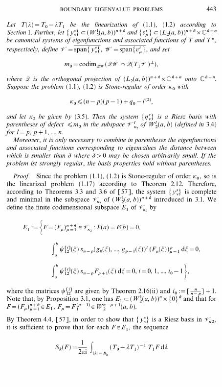
Theorem 5.2. Let the problem (1.1), (1.2) be non-degenerate, and let['s
&] be a corresponding canonical system of eigenfunctions and associatedfunctions. Suppose that fj # W j
� (a, b) for j=0, 1, ..., n&1, and that for somek # N, k�max[n& p+1, p&1] if p>0,
(i) fn&1& j # W k& j� (a, b) for j=0, 1, ..., n&1 if p=0 and k�n,
(ii) f0 , ..., fp&1 # W k&(n& p)� (a, b), fn&1& j # W k& j
� (a, b) for j=0, 1, ...,n& p&1 if k�n, and g0 , ..., gp&1 # W k
�(a, b) if p>0.
442 CHRISTIANE TRETTER
File: DISTL2 382936 . By:JB . Date:12:02:01 . Time:11:21 LOP8M. V8.B. Page 01:01Codes: 3033 Signs: 1778 . Length: 45 pic 0 pts, 190 mm
Let T(*)=T0&*T1 be the linearization of (1.1), (1.2) according toSection 1. Further, let [ ys
&]/(W 12(a, b))n+n and [v t
+ ]/(L2(a, b))n+n_C n+n
be canonical systems of eigenfunctions and associated functions of T and T*,respectively, define V=span[ ys
&], W=span[v t+ ], and set
m0=codimQW(QW & Q(T1 V)=),
where Q is the orthogonal projection of (L2(a, b))n+n_C n+n onto C n+n.Suppose the problem (1.1), (1.2) is Stone-regular of order }0 with
}0�(n& p)( p&1)+q0&l (2),
and let }2 be given by (3.5). Then the system [' s&] is a Riesz basis with
parentheses of defect �m0 in the subspace V l}2
of W l2(a, b) (defined in 3.4)
for l= p, p+1, ..., n.Moreover, it is only necessary to combine in parentheses the eigenfunctions
and associated functions corresponding to eigenvalues the distance betweenwhich is smaller than $ where $>0 may be chosen arbitrarily small. If theproblem ist strongly regular, the basis properties hold without parentheses.
Proof. Since the problem (1.1), (1.2) is Stone-regular of order }0 , so isthe linearized problem (1.17) according to Theorem 2.12. Therefore,according to Theorems 3.3 and 3.6 of [57], the system [ ys
&] is completeand minimal in the subspace V}2
of (W 12(a, b))n+n introduced in 3.1. We
define the finite codimensional subspace E1 of V}2by
E1 :={F=(F+)n+n+=1 # V}2
: F(a)=F(b)=0,
|b
a�[i]
12 (!) =n& p(g0(!), ..., gp&1(!))t (F+(!)) p+=1 d!=0,
|b
a�[i]
12 (!) =n& p Fp+1(!) d!=0, i=0, 1, ..., i0&1= ,
where the matrices �[i]12 are given by Theorem 2.16(ii) and i0 :=[ n
n& p]+1.Note that, by Proposition 3.1, one has E1 /(W 1
2(a, b))n_[0] n and that forF=(F+)n+n
+=1 # E1 , F+=F (+&1)1 # W n&++1
2 (a, b).
By Theorem 4.4, [57], in order to show that [ ys&] is a Riesz basis in V}2 ,
it is sufficient to prove that for each F # E1 , the sequence
Sk(F )=1
2?i ||*|=Rk
(T0&*T1)&1 T1F d*
443BOUNDARY EIGENVALUE PROBLEMS
File: DISTL2 382937 . By:JB . Date:12:02:01 . Time:11:21 LOP8M. V8.B. Page 01:01Codes: 3025 Signs: 1547 . Length: 45 pic 0 pts, 190 mm
converges unconditionally in the norm of (W 12(a, b))n+ n for k � �, where
(Rk)�1 /R+ is a sequence such that Rk � � for k � � and Rk {|*& | for
all k, &=1, 2, ... .
Now let F # E1 . Then W a1 F(a)+W b
1F(b)=0 and hence, by the formulas(2.6) and (2.7) from [57] for the resolvent of T,
S ( j)k (F )(x)=
12?i |
|*|=Rk
� j
�x j \(T0&*T1)&1 \A1F0 ++ (x) d*
=1
2?i ||*|=Rk
|b
a
� j
�x j G(x, !, *) A1(!) F(!) d! d*
=n& p2?i
:Mk
m=1|
�Gm|
b
a\n& p&1 � j
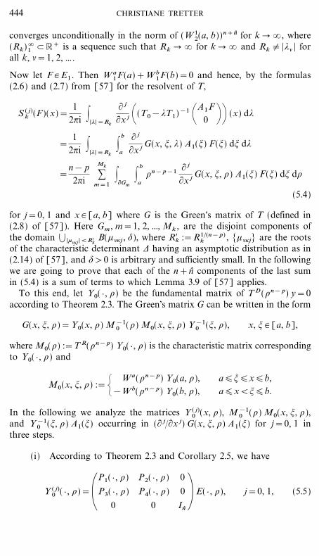
�x j G(x, !, \) A1(!) F(!) d! d\
(5.4)
for j=0, 1 and x # [a, b] where G is the Green's matrix of T (defined in(2.8) of [57]). Here Gm , m=1, 2, ..., Mk , are the disjoint components ofthe domain � |+&}j |<R$k
B(+&}j , $), where R$k :=R1�(n& p)k , [+&}j] are the roots
of the characteristic determinant 2 having an asymptotic distribution as in(2.14) of [57], and $>0 is arbitrary and sufficiently small. In the followingwe are going to prove that each of the n+n components of the last sumin (5.4) is a sum of terms to which Lemma 3.9 of [57] applies.
To this end, let Y0( } , \) be the fundamental matrix of T D(\n& p) y=0according to Theorem 2.3. The Green's matrix G can be written in the form
G(x, !, \)=Y0(x, \) M &10 (\) M0(x, !, \) Y &1
0 (!, \), x, ! # [a, b],
where M0(\) :=T R(\n& p) Y0( } , \) is the characteristic matrix correspondingto Y0( } , \) and
M0(x, !, \) :={ Wa(\n& p) Y0(a, \),&Wb(\n& p) Y0(b, \),
a�!�x�b,a�x<!�b.
In the following we analyze the matrices Y ( j)0 (x, \), M &1
0 (\) M0(x, !, \),and Y &1
0 (!, \) A1(!) occurring in (� j��x j) G(x, !, \) A1(!) for j=0, 1 inthree steps.
(i) According to Theorem 2.3 and Corollary 2.5, we have
P1( } , \) P2( } , \) 0
Y ( j)0 ( } , \)=\P3( } , \) P4( } , \) 0 + E( } , \), j=0, 1, (5.5)
0 0 In
444 CHRISTIANE TRETTER
File: DISTL2 382938 . By:JB . Date:12:02:01 . Time:11:21 LOP8M. V8.B. Page 01:01Codes: 2527 Signs: 766 . Length: 45 pic 0 pts, 190 mm
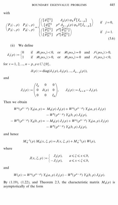
with
\P1( } , \)P3( } , \)
P2( } , \)P4( } , \)
={\[,[0]
11 ][,[0]
21
2p(\) .0V� [In& p]\ p 2n& p(\) .0V[In& p]+
\[,� [0]11 ]
[,� [0]21 ]
\ p[,� [0]12 ]
\n[,� [0]22 ]+
if j=0,
if j=1.
(5.6)
(ii) We define
$&(\) :={01
if R(\|&)<0, or R(\|&)=0 and I(\|&)>0,if R(\|&)>0, or R(\|&)=0 and I(\|&)<0,
for &=1, 2, ..., n& p, \ # C"[0],
$(\) :=diag($1(\), $2(\), ..., $n& p(\)),
and
Ip 0 0
J1(\) :=\ 0 $(\) 0 + , J2(\) :=In+ n&J1(\).
0 0 I n
Then we obtain
Wa(\n& p) Y0(a, \)= M0(\) J2(\)+Wa(\n& p) Y0(a, \) J1(\)
&Wb(\n& p) Y0(b, \) J2(\),
&Wb(\n& p) Y0(b, \)= &M0(\) J1(\)+Wa(\n& p) Y0(a, \) J1(\)
&Wb(\n& p) Y0(b, \) J2(\),
and hence
M &10 (\) M0(x, !, \)=J(x, !, \)+M &1
0 (\) W(\),
where
J(x, !, \) :={ J2(\),&J1(\),
a�!�x�b,a�x<!�b,
and
W(\) :=Wa(\n& p) Y0(a, \) J1(\)&Wb(\n& p) Y0(b, \) J2(\).
By (1.19), (1.22), and Theorem 2.3, the characteristic matrix M0(\) isasymptotically of the form
445BOUNDARY EIGENVALUE PROBLEMS

File: DISTL2 382939 . By:JB . Date:12:02:01 . Time:11:21 LOP8M. V8.B. Page 01:01Codes: 2917 Signs: 787 . Length: 45 pic 0 pts, 190 mm
446 CHRISTIANE TRETTER
M0(\
)
=
\Ba R\[,
[0
]11
(a)]
[,[
0]
21(a
)]2
p(\)
V�[I
n&
p]
\p
2n
&p(
\)V
[In
&p]++
Bb R\[,
[0
]11
(b)]
[,[
0]
21(b
)].
0(b
)2p(
\)V�
[In
&p]
E�n
&p(
b,\)
\p .
0(b
)2n
&p(
\)V
[In
&p]
E�n
&p(
b,\)+
W�a 0\[,
[0
]11
(a)]
[,[
0]
21(a
)]2
p(\)
V�[I
p]
\p
2n
&p(
\)V
[In
&p]++
W�b 0\[,
[0
]11
(b)]
[,[
0]
21(b
)].
0(b
)2p(
\)V�
[Ip]
E�n
&p(
b,\)
\p .
0(b
)2n&
p(\)
V[I
n&
p]
E�n&
p(b,
\)+}A
a R&
\n&
p
Ca R
+[V
]}}
}[V
]\l 1 (
[V]+
[V]
e\|
1(b
&a
) )}}
}\l 1 (
[V]+
[V]
e\|
n&p(
b&
a) )
&\n
&p
0
bb
bb
a 21
. ..
bb
bb
b. .
.
[V]
}}}
[V]
\l n ([V
]+[V
]e\
|1(
b&
a) )
}}}
\l n ([V
]+[V
]e\
|n&
p(b
&a
) )a n
1}}
}a n
,n
&1
&\n
&p
=
\+,
[V]
}}}
[V]
\l n+1 (
[V]+
[V]
e\|
1(b
&a
)}}
}\l n+
1 ([V
]+[V
]e\
|n&
p(b
&a
) )
Ca R
bb
bb
bb
bb
[V]
}}}
[V]
\l n+n (
[V]+
[V]
e\|
1(b
&a
) )}}
}\l n+
n ([V
]+[V
]e\
|n&
p(b
&a
) )
whe
reth
eex
pone
nts
l 1,l
2,.
..,l n
+n
are
asin
Def
init
ion
5.1,
(aij)n i,
j=1
:=A
a Ran
dV
stan
dsfo
ren
trie
sw
hich
dono
tde
pend
on\
and
need
not
besp
ecifi
ed.

File: DISTL2 382940 . By:JB . Date:12:02:01 . Time:11:21 LOP8M. V8.B. Page 01:01Codes: 1864 Signs: 315 . Length: 45 pic 0 pts, 190 mm
447BOUNDARY EIGENVALUE PROBLEMS
The
asym
ptot
icst
ruct
ure
ofW
(\)
is
[V]
}}}
[V]
\l 1 [V]
e�p+
1(a,
\)
}}}
\l 1 [V]
e�n(
a,\
)&
\n&p
0
bb
bb
a 21
. ..
bb
bb
b. .
.
[V]
}}}
[V]
\l n [V]
e�p+
1(a,
\)
}}}
\l n [V]
e�n(
a,\
)a n
1}}
}a n
,n&
1&
\n&p
W(\
)=
\+,
[V]
}}}
[V]
\l n+1 [
V]e�
p+1(
a,\
)}}
}\l n+
1 [V]
e�n(
a,\
)
Ca R
bb
bb
bb
bb
[V]
}}}
[V]
\l n+n [
V]e�
p+1(
a,\
) )}}
}\l n+
n [V]
e�n(
a,\
) )

File: DISTL2 382941 . By:JB . Date:12:02:01 . Time:11:12 LOP8M. V8.B. Page 01:01Codes: 3051 Signs: 1350 . Length: 45 pic 0 pts, 190 mm
where the function �&( } , \), &= p+1, ..., n, \ # C"[0], is defined as
�&(x, \) :={\|&& p(b&x) if R(\|&& p)<0,
or R(\|&& p)=0 and I(\|&& p)>0,&\|&& p(x&a) if R(\|&& p)>0,
or R(\|&& p)=0 and I(\|&& p)<0,
for x # [a, b]. Note that R(�&(x, \))�0 for all x # [a, b] and \ # C"[0]. If welet
M0(\)=: (m1(\) } } } mn+n(\)) , W(\)=: (w1(\) } } } wn+n(\)),
then, by Cramer's rule,
M&10 (\) M0(x, !, \)
=J(x, !, \)+\ 120(\)
det(m1(\) } } } m&&1(\) w+(\)
m&+1(\) } } } mn+n(\))n+n&, +=1)
M1(x, !, \) M2(x, !, \) M3(x, !, \)
=\M4(x, !, \) M5(x, !, \) M6(x, !, \)+ . (5.7)
M7(x, !, \) M8(x, !, \) M9(x, !, \)
By (2.7), the characteristic determinant 20(\)=det(T R(\n& p) Y0( } , \)) is ofthe form
20(\)=\(n& p)( p&1) 2(\),
where 2(\)=det(T R(\n& p) Y( } , \)) with Y( } , \) being the fundamentalmatrix of T D(\n& p) y=0 according to Theorem 2.2 and Remark 2.4 of [57]with C(\) as in Proposition 2.1. Since the problem (1.1), (1.2) is Stone-regular,the zeros of 20(\) have an asymptotic distribution of the form (2.14) of [57](see Proposition 2.10 of [57]).
Then, together with the asymptotic expansion of 2(\) stated in Proposi-tion 2.6 of [57] and the Stone-regularity of order }0 , we obtain, setting}~ 0 :=}0+l(2)&q0 ,
M1(x, !, \)={ \}~ 0&(n& p)( p&1)([V] S&+(\)) p&, +=1 ,
&Ip+\}~ 0&(n& p)( p&1)([V] S&+(\)) p&, +=1 ,
a�!�x�b,a�x<!�b,
M2(x, !, \)=\}~ 0&(n& p)( p&1)+l (1)&l (2)(e�+(a, \)[V] S&+(\)) p
&=1,n
+= p+1 ,
M3(x, !, \)=0p_n ,
M4(x, !, \)=\}~ 0&(n& p)( p&1)+l (3)&l (2)(e�&(b, \)[V] S&+(\)) n
&= p+1,p
+=1 ,
448 CHRISTIANE TRETTER
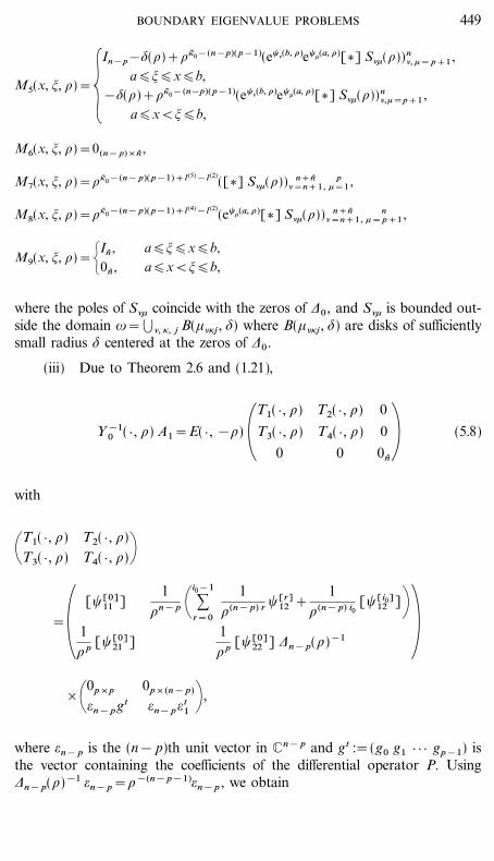
File: DISTL2 382942 . By:JB . Date:12:02:01 . Time:11:12 LOP8M. V8.B. Page 01:01Codes: 2673 Signs: 992 . Length: 45 pic 0 pts, 190 mm
M5(x, !, \)={In&p&$(\)+\}~ 0&(n&p)( p&1)(e�&(b, \)e�+(a, \)[V] S&+(\))n
&, += p+1 ,a�!�x�b,
&$(\)+\}~ 0&(n&p)( p&1)(e�&(b, \)e�+(a, \)[V] S&+(\))n&,+=p+1 ,
a�x<!�b,
M6(x, !, \)=0(n& p)_n ,
M7(x, !, \)=\}~ 0&(n& p)( p&1)+l (5)&l (2)([V] S&+(\)) n+n
&=n+1,p
+=1 ,
M8(x, !, \)=\}~ 0&(n& p)( p&1)+l (4)&l (2)(e�+(a, \)[V] S&+(\)) n+n
&=n+1,n
+= p+1 ,
M9(x, !, \)={In ,0n ,
a�!�x�b,a�x<!�b,
where the poles of S&+ coincide with the zeros of 20 , and S&+ is bounded out-side the domain |=�&, }, j B(+&}j , $) where B(+&}j , $) are disks of sufficientlysmall radius $ centered at the zeros of 20 .
(iii) Due to Theorem 2.6 and (1.21),
T1( } , \) T2( } , \) 0
Y&10 ( } , \) A1=E( } , &\) \T3( } , \) T4( } , \) 0 + (5.8)
0 0 0n
with
\T1( } , \) T2( } , \)T3( } , \) T4( } , \)+
=\[�[0]
11 ]
1\ p [�[0]
21 ]
1\n& p \ :
i0&1
r=0
1\(n& p) r �[r]
12 +1
\(n& p) i0[�[i0]
12 ]+1\p [�[0]
22 ] 2n& p(\)&1 +_\0p_p
=n& pgt
0p_(n& p)
=n& p=t1 + ,
where =n& p is the (n& p)th unit vector in Cn& p and gt :=(g0 g1 } } } gp&1) isthe vector containing the coefficients of the differential operator P. Using2n& p(\)&1 =n& p=\&(n& p&1)=n& p , we obtain
449BOUNDARY EIGENVALUE PROBLEMS
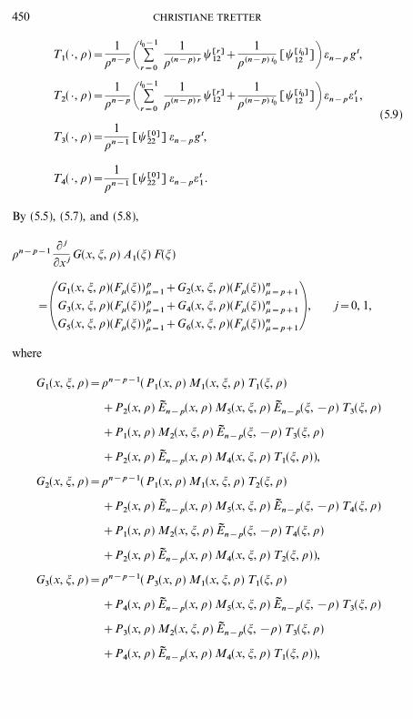
File: DISTL2 382943 . By:JB . Date:12:02:01 . Time:11:12 LOP8M. V8.B. Page 01:01Codes: 2764 Signs: 877 . Length: 45 pic 0 pts, 190 mm
T1( } , \)=1
\n& p \ :i0&1
r=0
1\(n& p) r �[r]
12 +1
\(n& p) i0[�[i0]
12]+ =n& p gt,
T2( } , \)=1
\n& p \ :i0&1
r=0
1\(n& p) r �[r]
12 +1
\(n& p) i0[�[i0]
12 ]+ =n& p=t1 ,
(5.9)
T3( } , \)=1
\n&1 [�[0]22 ] =n& p gt,
T4( } , \)=1
\n&1 [�[0]22 ] =n& p=t
1 .
By (5.5), (5.7), and (5.8),
\n& p&1 � j
�x j G(x, !, \) A1(!) F(!)
G1(x, !, \)(F+(!)) p+=1+G2(x, !, \)(F+(!))n
+= p+1
=\G3(x, !, \)(F+(!)) p+=1+G4(x, !, \)(F+(!))n
+= p+1+ , j=0, 1,
G5(x, !, \)(F+(!)) p+=1+G6(x, !, \)(F+(!))n
+= p+1
where
G1(x, !, \)=\n& p&1( P1(x, \) M1(x, !, \) T1(!, \)
+P2(x, \) E� n& p(x, \) M5(x, !, \) E� n& p(!, &\) T3(!, \)
+P1(x, \) M2(x, !, \) E� n& p(!, &\) T3(!, \)
+P2(x, \) E� n& p(x, \) M4(x, !, \) T1(!, \)),
G2(x, !, \)=\n& p&1( P1(x, \) M1(x, !, \) T2(!, \)
+P2(x, \) E� n& p(x, \) M5(x, !, \) E� n& p(!, &\) T4(!, \)
+P1(x, \) M2(x, !, \) E� n& p(!, &\) T4(!, \)
+P2(x, \) E� n& p(x, \) M4(x, !, \) T2(!, \)),
G3(x, !, \)=\n& p&1( P3(x, \) M1(x, !, \) T1(!, \)
+P4(x, \) E� n& p(x, \) M5(x, !, \) E� n& p(!, &\) T3(!, \)
+P3(x, \) M2(x, !, \) E� n& p(!, &\) T3(!, \)
+P4(x, \) E� n& p(x, \) M4(x, !, \) T1(!, \)),
450 CHRISTIANE TRETTER

File: DISTL2 382944 . By:JB . Date:12:02:01 . Time:11:12 LOP8M. V8.B. Page 01:01Codes: 2913 Signs: 1336 . Length: 45 pic 0 pts, 190 mm
G4(x, !, \)=\n& p&1( P3(x, \) M1(x, !, \) T2(!, \)
+P4(x, \) E� n& p(x, \) M5(x, !, \) E� n& p(!, &\) T4(!, \)
+P3(x, \) M2(x, !, \) E� n& p(!, &\) T4(!, \)
+P4(x, \) E� n& p(x, \) M4(x, !, \) T2(!, \)),
G5(x, !, \)=\n& p&1(M7(x, !, \) T1(!, \)
+M8(x, !, \) E� n& p(!, &\) T3(!, \)),
G6(x, !, \)=\n& p&1(M7(x, !, \) T2(!, \)
+M8(x, !, \) E� n& p(!, &\) T4(!, \)).
According to Lemma 3.9 of [57], we distinguish: (a) the terms without anyexponentials, (b) those with exponentials only in x and only in !, and (c)those with exponentials in x as well as in !. Then the highest possible \-poweris &2 in case (a), &1 in case (b) and 0 in case (c).
(a) Terms Containing Neither E� n& p(x, \) nor E� n& p(!, &\). Using (5.6),(5.9), the asymptotic structure of M1(x, !, \), and F # E1 , we find
=t& \n& p&1 |
b
aP1(x, \) M1(x, !, \) T1(!, \)(F+(!)) p
+=1 d!
=V(x, \)+ :p
+=1
:p
k=1
:p
l=1|
b
a\}~ 0&1&( p&1+i0)(n& p)
_[V1, &l(x)] Slk(\)[V1, k+(!)] F+(!) d!
and, since =t1(F+)n
+= p+1=Fp+1 ,
=t& \n& p&1 |
b
aP1(x, \) M1(x, !, \) T2(!, \)(F+(!))n
+= p+1 d!
=V(x, \)+ :p
k=1
:p
l=1|
b
a\}~ 0&1&( p&1+i0)(n& p)
_[V1, &l(x)] Slk(\)[V2, k, p+1(!)] Fp+1(!) d!
for &=1, 2, ..., p, where V(x, \) denotes a term which is holomorphic in \ andhence does not contribute to the integration with respect to \. The terms con-taining P3(x, \) M1(x, !, \) Ti(!, \), i=1, 2, have analogous representations.By the assumption on }0 and since i0=[ n
n& p]+1, we have
}~ 0&1&( p&1+i0)(n& p)�&1&i0(n& p)�&1&n�&2. (5.10)
451BOUNDARY EIGENVALUE PROBLEMS
File: DISTL2 382945 . By:JB . Date:12:02:01 . Time:11:12 LOP8M. V8.B. Page 01:01Codes: 2706 Signs: 991 . Length: 45 pic 0 pts, 190 mm
Hence Lemma 3.9 of [57] can be applied to the corresponding sums ofintegrals over Gm in (5.4). The same reasoning is used for
et&\n& p&1 |
b
aM7(x, !, \) T1(!, \)(F+(!)) p
+=1 d!
= :p
+=1
:p
k=1|
b
a\}~ 0&1&(p&1+i0)(n& p)+l (5)&l (2)S&k(\)[V1, k+(!)] F+(!) d!
and
et& \n& p&1 |
b
aM7(x, !, \) T2(!, \)(F+(!))n
+= p+1 d!
= :p
k=1|
b
a\}~ 0&1&(p&1+i0)(n& p)+l (5)&l (2)S&k(\)[V2, k, p+1(!)] Fp+1(!) d!,
where &=1, 2, ..., n, because l (5)&l (2)�0.
(b) Terms Containing E� n& p(x, \) Only. Again, using the fact thatF # E1 , we obtain
=t& \n& p&1 |
b
aP2(x, \) E� n& p(x, \) M4(x, !, \) T1(!, \)(F+(!)) p
+=1 d!
= :p
+=1
:p
k=1
:n
l= p+1|
b
a\}~ 0&1&( p&1+i0)(n& p)+l (3)&l (2)+ p[V2, &l (x)]
_e�l(a+b&x, \)Slk(\)[V1, k+(!)] F+(!) d!
for &=1, 2, ..., p and
=t&& p \n& p&1 |
b
aP4(x, \) E� n& p(x, \) M4(x, !, \) T1(!, \)(F+(!)) p
+=1 d!
= :p
+=1
:p
k=1
:n
l= p+1|
b
a\}~ 0&1&( p&1+i0)(n& p)+l (3)&l (2)+n[V4, &l(x)]
_e�l (a+b&x, \)Slk(\)[V1, k+(!)] F+(!) d!
for &= p+1, ..., n. Here the assumptions of Lemma 3.9 of [57] are fulfilledbecause
}~ 0&1&( p&1+i0)(n& p)+l (3)&l (2)+ p
<}~ 0&1&( p&1+i0)(n& p)+l (3)&l (2)+n
�}~ 0&1&( p&1+i0)(n& p)+n
�&1
452 CHRISTIANE TRETTER

File: DISTL2 382946 . By:JB . Date:12:02:01 . Time:11:12 LOP8M. V8.B. Page 01:01Codes: 2749 Signs: 1173 . Length: 45 pic 0 pts, 190 mm
since l (3)&l (2)�0 and by the estimate (5.10). For the terms containingPi(x, \) E� n& p(x, \) M4(x, !, \) T2(!, \), i=2, 4, we proceed in the same way.
Terms Containing E� n& p(!, &\) Only. Integrating by parts n& p timeswith respect to !, using
E� n& p(!, &\)=dd! \&
1\
0&1n& pE� n& p(!, &\)+ ,
we obtain
=t& \n& p&1 |
b
aP1(x, \) M2(x, !, \) E� n& p(!, &\) T3(!, \)(F+(!)) p
+=1 d!
==t& \n& p&1P1(x, \) M2(\) |
b
a
1\n& p 0&(n& p)
n& p E� n& p(!, &\)
_ :n& p
s=0\n& p
s + dn& p&s
d!n& p&s T3(!, \)(F (s)+ (!)) p
+=1 d!
for &=1, 2, ..., p, where M2(\)=M2(x, !, \) is independent of x and !. Herewe have used the fact that F (s)
+ =F (+&1+s)1 # W n&(++s)+1
2 (a, b)/W 12(a, b) for
s=0, 1, ..., n& p, +=1, 2, ..., p, and that, in addition, F (s)+ (a)=F (s)
+ (b)=0 fors=0, 1, ..., n& p&1, +=1, 2, ..., p, because F # E1 . By (5.8) and Corollary 2.7,it follows that
dn& p&s
d!n& p&s T3(!, \)=dn& p&s
d!n& p&s (�22(!, \) =n& pg(!)t)
= :n& p&s
t=0\n& p&s
t + dt
d!t (�22(!, \) =n& p) g(n& p&s&t)(!)t
=1
\n&1 ([V3, s, k+(!)]) nk= p+1,
p+=1 .
Together with the asymptotic representations of P1(x, \) in (5.6) and ofM2(\)=M2(x, !, \), one has
=t& \n& p&1 |
b
aP1(x, \) M2(x, !, \) E� n& p(!, &\) T3(!, \)(F+(!)) p
+=1 d!
= :p
+=1
:n
k= p+1
:p
l=1|
b
a\}~ 0&( p&1)(n& p)+l (1)&l (2)&n[V1, &l (x)]
_Slk(\)1
|n& pk& p
e�k(!, \) :n& p
s=0
[V3, s, k+(!)] F (s)+ (!) d!
453BOUNDARY EIGENVALUE PROBLEMS
File: DISTL2 382947 . By:JB . Date:12:02:01 . Time:11:12 LOP8M. V8.B. Page 01:01Codes: 3252 Signs: 1439 . Length: 45 pic 0 pts, 190 mm
for &=1, 2, ..., p. In order to apply Lemma 3.9 of [57] to the term resultingin (5.4), we observe that l (2)&l (1)�n&1 and hence }~ 0&( p&1)(n& p)+l (1)
&l (2)&n�&1 by the assumption on }0 . The terms arising from P1(x, \)M2(x, !, \) E� n& p(!, &\) T4(!, \) and from P3(x, \) M2(x, !, \) E� n& p(!, &\)Ti(!, \), i=3, 4, can be treated analogously if we observe thatT4(!, \)=�22(!, \) =n& p=t
1 , F (s)p+1=F ( p+s)
1 # W n&(s+ p)2 (a, b)/L2(a, b) for
s=0, 1, ..., n& p and F (s)p+1(a)=F (s)
p+1(b)=0 for s=0, 1, ..., n& p&1 becauseF # E1 . Also, we have
et&\n& p&1 |
b
aM8(x, !, \) E� n& p(!, &\) T3(!, \)(F+(!)) p
+=1 d!
= :p
+=1
:n
k= p+1|
b
a\}~ 0&( p&1)(n& p)+l (4)&l (2)&nS&k(\)
_1
|n& pk& p
e�k(!, \) :n& p
s=0
[V3, s, k+(!)] F (s)+ (!) d!
for &=1, 2, ..., n. Here Lemma 3.9 of [57] can be applied because we have theestimate l (4)�l (1)&(n& p)<l (1) and hence }~ 0&( p&1)(n& p)+l (4)&l (2)&n<}~ 0&( p&1)(n& p)+l (1)&l (2)&n�&1 again by assumption. The samereasoning is used for M8(x, !, \) E� n& p(!, &\) T4(!, \).
(c) Terms Containing E� n& p(x, \) as Well as E� n& p(!, &\). Integrationby parts n& p times with respect to ! as before yields
=t& \n& p&1 |
b
aP2(x, \) E� n& p(x, \) M5(x, !, \)
_E� n& p(!, &\) T3(!, \)(F+(!)) p+=1 d!
=V(x, \)+ :p
+=1
:n
k= p+1
:n
l= p+1|
b
a\}~ 0&(n& p)( p&1)&(n& p)[V2, &l (x)]
_e�l (a+b&x, \)Slk(\)1
|n& pk& p
e�k(!, \) :n& p
s=0
[V3, s, k+(!)] F (s)+ (!) d!
for &=1, 2, ..., p and
=t&& p \n& p&1 |
b
aP4(x, \) E� n& p(x, \) M5(x, !, \)
_E� n& p(!, &\) T3(!, \)(F+(!)) p+=1 d!
=V(x, \)+ :p
+=1
:n
k= p+1
:n
l= p+1|
b
a\}~ 0&(n& p)( p&1)[V4, &l (x)]
_e�l(a+b&x, \)Slk(\)1
|n& pk& p
e�k(!, \) :n& p
s=0
[V3, s, k+(!)] F (s)+ (!) d!
454 CHRISTIANE TRETTER
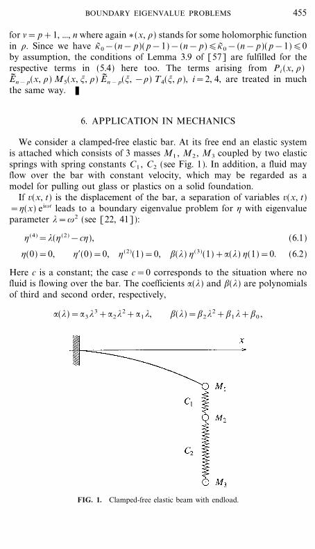
for &= p+1, ..., n where again V (x, \) stands for some holomorphic functionin \. Since we have }~ 0&(n& p)( p&1)&(n& p)�}~ 0&(n& p)( p&1)�0by assumption, the conditions of Lemma 3.9 of [57] are fulfilled for therespective terms in (5.4) here too. The terms arising from Pi (x, \)E� n& p(x, \) M5(x, !, \) E� n& p(!, &\) T4(!, \), i=2, 4, are treated in muchthe same way. K
6. APPLICATION IN MECHANICS
We consider a clamped-free elastic bar. At its free end an elastic systemis attached which consists of 3 masses M1 , M2 , M3 coupled by two elasticsprings with spring constants C1 , C2 (see Fig. 1). In addition, a fluid mayflow over the bar with constant velocity, which may be regarded as amodel for pulling out glass or plastics on a solid foundation.
If v(x, t) is the displacement of the bar, a separation of variables v(x, t)='(x) ei|t leads to a boundary eigenvalue problem for ' with eigenvalueparameter *=|2 (see [22, 41]):
'(4)=*('(2)&c'), (6.1)
'(0)=0, '$(0)=0, '(2)(1)=0, ;(*) '(3)(1)+:(*) '(1)=0. (6.2)
Here c is a constant; the case c=0 corresponds to the situation where nofluid is flowing over the bar. The coefficients :(*) and ;(*) are polynomialsof third and second order, respectively,
:(*)=:3*3+:2*2+:1*, ;(*)=;2*2+;1 *+;0 ,
FIG. 1. Clamped-free elastic beam with endload.
455BOUNDARY EIGENVALUE PROBLEMS
File: DISTL2 382949 . By:JB . Date:12:02:01 . Time:11:12 LOP8M. V8.B. Page 01:01Codes: 2545 Signs: 1006 . Length: 45 pic 0 pts, 190 mm
where
:3=M1 M2M3 ,
:2=&(C1 M2 M3+M1(C2 M2+C1M3+C2M3)),
:1=C1(C2M2+C1M3+C2 M3)+C1C2M1&C 21 M3 ,
and
;2=M2M3 ,
;1=&(C2 M2+C1M3+C2 M3),
;0=C1 C2 .
Here M1 , M2 , M3>0 and C1 , C2>0 are dimensionless constants standingfor the masses and spring constants of the system.
6.1. Regularity
First we have to check the regularity of the problem (6.1), (6.2). For thispurpose we have to calculate an asymptotic fundamental matrix of thecorresponding first order system of differential equations according toTheorem 2.2 of [57]. Here a transformation of this system is required inorder to make the coefficient of * diagonal.
Theorem 6.1. The problem (6.1), (6.2) is Stone-regular of order 0.
Proof. By means of the substitution y1=', y2='$, y3='(2), y4='(3),y~ =( yi)
4i=1 , the fourth order problem (6.1), (6.2) is equivalent to the first
order boundary eigenvalue problem T� (*) y~ =(T� D(*), T� R(*))t y~ =0 where
T� D(*) y~ =y~ $+\0000
&1000
0&1
00
00
&10+ y~ &* \
000c
0000
0001
0000+ y~ ,
T� R(*) y~ =\0010
0001
0000
0000+ y~ (0)+\
:(*)000
0000
0100
;(*)000 + y~ (1).
456 CHRISTIANE TRETTER

File: DISTL2 382950 . By:JB . Date:12:02:01 . Time:11:12 LOP8M. V8.B. Page 01:01Codes: 2778 Signs: 843 . Length: 45 pic 0 pts, 190 mm
First we transform this system in such a way that Assumption 2.1 of [57]is fulfilled. According to Section 2, we substitute *=\2, and |1=1,|2=&1 denote the square roots of 1. Further,
V=\11
1&1+ , 22(\)=\1
00\+ , 0=\0
10
&1+ .
The matrix C� (\) defined in (2.3) and its inverse are given by
C� (\)=\1000
0100
01\\2
0&1\
&\2+ , C� (\)&1=\1 0 0 0
+ .
0 1 0 &1\2
0 01
2\1
2\2
0 01
2\&
12\2
Then the transformed operator T� D(\)=C� (\)&1 T� D(\2) C� (\) is of theform T� D(\) y~ = y~ $&A� ( } , \) y~ where
A� ( } , \)=\ \0000
0000
0010
000
&1++\0 1 1 &1
+=\A� 1+A� 0 .
&c 0 0 0
c2
0 0 0
&c2
0 0 0
Hence all conditions of Assumption 2.1 of [57] are satisfied with k # N0
arbitrarily large. Then Theorem 2.2 of [57] yields an asymptoticfundamental matrix Y� ( } , \) of the transformed system T� D(\) y~ =0 which isgiven by
Y� (x, \)=\\1000
x100
0010
0001++\&1 \
0000
0000
1000
1000++O(\&2)+
_\1000
0100
00
e \x
0
000
e&\x+
457BOUNDARY EIGENVALUE PROBLEMS

File: DISTL2 382951 . By:JB . Date:12:02:01 . Time:11:12 LOP8M. V8.B. Page 01:01Codes: 2786 Signs: 910 . Length: 45 pic 0 pts, 190 mm
if c=0 and by
Y� (x, \)=\\cos(- c x) &
1
- csin(- c x) 0 0
+- c sin(- c x) cos(- cx) 0 0
0 0 1 0
0 0 0 1
+\&1\0 0 1 1
++O(\&2)+0 0 0 0
&c2
cos(- c x)- c2
sin(- c x) 0 0
&c2
cos(- c x)- c2
sin(- cx) 0 0
_\1000
0100
00
e\x
0
000
e&\x+if c{0. After some calculations, one finds that the characteristic determinant
2� (\)=det(W� 0(\2) C� (\) Y� (0, \)+W� 1(\2) C� (\) Y� (1, \))
has an asymptotic expansion
2� (\)={\7([&:3]1 e\+[2;2]1+[&:3]1 e&\) if c=0,
\7 \_:3
sin - c
- c &1
e\+[2;2]1+_:3
sin - c
- c &1
e&\+ if c{0.
According to (2.11) and (2.10), we have
q~ 1=6, q~ 2=1, q~ 3=0, q~ 4=0, q~ 0=q~ 1+ } } } +q~ 4=7.
Then the smallest polygon M containing the points figuring as exponentse\ } in 2� (\) is given by M=[&1, 1], and M0=[&1, 1]. Hence, by Defini-tion 2.10, the problem (6.1), (6.2) is Stone-regular of order 0. K
6.2. Linearization of the Problem
Since the boundary conditions (6.2) depend polynomially on the eigen-value parameter, the problem (6.1), (6.2) can be linearized along the lines
458 CHRISTIANE TRETTER

File: DISTL2 382952 . By:JB . Date:12:02:01 . Time:11:12 LOP8M. V8.B. Page 01:01Codes: 1858 Signs: 578 . Length: 45 pic 0 pts, 190 mm
of Section 1. The dimension of the linearized first order system is increasedby the total polynomial degree n=3 of the boundary conditions (6.2) to 7and reads as follows.
Theorem 6.2. The boundary eigenvalue problem (6.1), (6.2) for' # W 4
2(0, 1) is equivalent to the *-linear first order boundary eigenvalueproblem
0 &1 0 0 0 0 00 0 &1 0 0 0 00 0 0 &1 0 0 0
y$+\0 0 0 0 0 0 0+ y0 0 0 0 0 0 00 0 0 0 0 0 00 0 0 0 0 0 0
0 0 0 0 0 0 00 0 0 0 0 0 00 0 0 0 0 0 0
=*\ c 0 1 0 0 0 0+ y,0 0 0 0 0 0 00 0 0 0 0 0 00 0 0 0 0 0 0
0 0 0 0 &* 0 00 0 0 0 1 &* 00 0 0 0 0 1 &*\0 0 0 0 0 0 1+ y(0)0 0 0 0 0 0 01 0 0 0 0 0 00 1 0 0 0 0 0
0 0 0 ;0 0 0 0:1 0 0 ;1 0 0 0:2 0 0 ;2 0 0 0
+\:3 0 0 0 0 0 0+ y(1)=00 0 1 0 0 0 00 0 0 0 0 0 00 0 0 0 0 0 0
459BOUNDARY EIGENVALUE PROBLEMS

File: DISTL2 382953 . By:JB . Date:12:02:01 . Time:11:12 LOP8M. V8.B. Page 01:01Codes: 2237 Signs: 531 . Length: 45 pic 0 pts, 190 mm
for y=( yi)7i=1 # (W 1
2(0, 1))7 where y1=', y2='$, y3='(2), andy4='(3).
Proof. In order to determine the linearization of the problem (6.1),(6.2), we need the following quantities introduced in Section 1:
m1=3, m2=0, m3=0, m4=0,
n=3,
l=3,
+0=3, +1= 0, +2= 0, +3=1,
k0=4, k1= 1, k2= 1, k3=1, k4=0.
Then, by the definitions in Section 1,
C(*)&1=\*&3
000
0100
0010
0001+ , W� a
C(*)=W� a0=\
0010
0001
0000
0000+ ,
W� bC(*)=W� b
0+*&1W� b1+*&2W� b
2+*&3W� b3
=\:3
000
0000
0100
0000++*&1 \
:2
000
0000
0000
;2
000 +
+*&2 \:1
000
0000
0000
;1
000 ++*&3 \
0000
0000
0000
;0
000 + ,
460 CHRISTIANE TRETTER

File: DISTL2 382954 . By:JB . Date:12:02:01 . Time:11:12 LOP8M. V8.B. Page 01:01Codes: 2689 Signs: 1078 . Length: 45 pic 0 pts, 190 mm
0 0 0
P3=(1 0 0 0), AaR=\1 0 0+ , C a
R=\0000
0000
1000+ ,
0 1 0
P3W� a3 0 0 0 0
B aR=\P3W� a
2+=\0 0 0 0+ ,
P3W� a1 0 0 0 0
P3W� b3 0 0 0 ;0
B bR=\P3W� b
2+=\:1 0 0 ;1+ .
P3W� b1 :2 0 0 ;2
Note that P1 , P2 do not appear since +1=+2=0. Together with theformulas in (1.22) the assertion follows. K
6.3. Completeness Result
According to Theorem 6.1, the problem (6.1), (6.2) fulfills the regularityassumptions of the completeness theorem in Section 3. If we apply thistheorem and calculate the spaces V l
k figuring therein, we obtain the follow-ing completeness result for the boundary eigenvalue problem of the elasticbar:
Theorem 6.3. Each canonical system of eigenfunctions and associatedfunctions of the boundary eigenvalue problem (6.1), (6.2) is complete in thespaces
V 03=L2(0, 1),
V 13=[' # W 1
2(0, 1) : '(0)=0],
V 23=[' # W 2
2(0, 1) : '(0)=0, '$(0)=0],
V 33=[' # W 3
2(0, 1) : '(0)=0, '$(0)=0, '"(1)=0],
V 43=[' # W 4
2(0, 1) : '(0)=0, '$(0)=0, '"(1)=0].
Proof. By Theorem 3.5 and Theorem 6.1, the eigenfunctions andassociated functions of problem (6.1), (6.2) are complete in the subspacesV l
3 /W l2(0, 1) for l=0, 1, ..., 4, since, by (3.5),
461BOUNDARY EIGENVALUE PROBLEMS

File: DISTL2 382955 . By:JB . Date:12:02:01 . Time:11:12 LOP8M. V8.B. Page 01:01Codes: 2151 Signs: 768 . Length: 45 pic 0 pts, 190 mm
}2=_}0
2 &+3=3.
In order to determine the spaces V l3 according to (3.4), we first have to
calculate the space V3 (see (3.1)) associated with the linearized problem.From Theorem 6.2, where the linearized problem was stated, we find thatthe operators T0 , T1 : (W 1
2(0, 1))7 � (L2(0, 1))7_C7 in (1.17) are given by
T0y=\y$1& y2
+ ,
y$2& y3
y$3& y4
y$4y$5y$6y$7
;0 y4(1)
y5(0)+:1y1(1)+;1 y4(1)
y6(0)+:2y1(1)+;2 y4(1)
y7(0)+:3y1(1)
y3(1)
y1(0)
y2(0)
T1y=\0
+ ,
0
0
cy1+ y3
0
0
0
y5(0)
y6(0)
y7(0)
0
0
0
0
for y=( yi )7i=1 # (W 1
2(0, 1))7. To determine the operator A=T1T &10 acting
in (L2(0, 1))7_C7, we let (v, c)t # (L2(0, 1))7_C7 where v=(vi)7i=1 ,
c=(ci)7i=1 . Then T &1
0 (v, c)t=( yi)7i=1 is given by
y1(x)=|x
0v1(t) dt+|
x
0|
t
0v2({) d{ dt&|
x
0|
t
0|
1
{v3(') d' d{ dt
+|x
0|
t
0|
1
{|
1
'v4(+) d+ d' d{ dt
+1
6;0
x2(x&3) c1+12
x2c5+xc7+c6 ,
462 CHRISTIANE TRETTER
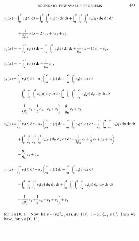
File: DISTL2 382956 . By:JB . Date:12:02:01 . Time:11:12 LOP8M. V8.B. Page 01:01Codes: 1987 Signs: 621 . Length: 45 pic 0 pts, 190 mm
y2(x)=|x
0v2(t) dt&|
x
0|
1
tv3({) d{ dt+|
x
0|
1
t|
1
{v4(') d' d{ dt
+1
2;0
x(x&2) c1+xc5+c7 ,
y3(x)=&|1
xv3(t) dt+|
1
x|
1
tv4({) d{ dt+
1;0
(x&1) c1+c5 ,
y4(x)=&|1
xv4(t) dt+
1;0
c1 ,
y5(x)=|x
0v5(t) dt&:1 \|
1
0v1(t) dt+|
1
0|
t
0v2({) d{ dt
&|1
0|
t
0|
1
{v3(') d' d{ dt |
1
0|
t
0|
1
{|
1
'v4(+) d+ d' d{ dt
&1
3;0
c1+12
c5+c6+c7+&;1
;0
c1+c2 ,
y6(x)=|x
0v6(t) dt&:2 \|
1
0v1(t) dt+|
1
0|
t
0v2({) d{ dt&|
1
0|
t
0|
1
{v3(') d' d{ dt
+|1
0|
t
0|
1
{|
1
'v4(+) d+ d' d{ dt&
13;0
c1+12
c5+c6+c7+&
;2
;0
c1+c3 ,
y7(x)=|x
0v7(t) dt&:3 \|
1
0v1(t) dt+|
1
0|
t
0v2({) d{ dt
&|1
0|
t
0|
1
{v3(') d' d{ dt+|
1
0|
t
0|
1
{|
1
'v4(+) d+ d' d{ dt
&1
3;0
c1+12
c5+c6+c7++c4
for x # [0, 1]. Now let v=(vi)7i=1 # (L2(0, 1))7, c=(ci)
7i=1 # C7. Then we
have, for x # [0, 1],
463BOUNDARY EIGENVALUE PROBLEMS
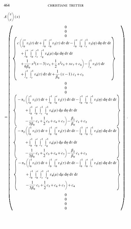
File: DISTL2 382957 . By:JB . Date:12:02:01 . Time:11:12 LOP8M. V8.B. Page 01:01Codes: 2307 Signs: 509 . Length: 45 pic 0 pts, 190 mm
A \vc+ (x)
= .
000
{c \|
x
0v1(t) dt+|
x
0|
t
0v2({) d{ dt&|
x
0|
t
0|
1
{v3(') d' d{ dt
=+|x
0|
t
0|
1
{|
1
'v4(+) d+ d' d{ dt
+1
6;0
x2(x&3) c1+12
x2c5+xc7+c6+&|1
xv3(t) dt
+|1
x|
1
tv4({) d{ dt+
1;0
(x&1) c1+c5
000
&:1 \|1
0v1(t) dt+|
1
0|
t
0v2({) d{ dt&|
1
0|
t
0|
1
{v3(') d' d{ dt
{ +|1
0|
t
0|
1
{|
1
'v4(+) d+ d' d{ dt =&
13;0
c1+12
c5+c6+c7+&;1
;0
c1+c2
&:2 \|1
0v1(t) dt+|
1
0|
t
0v2({) d{ dt&|
1
0|
t
0|
1
{v3(') d' d{ dt
{ +|1
0|
t
0|
1
{|
1
'v4(+) d+ d' d{ dt =&
13;0
c1+12
c5+c6+c7+&;2
;0
c1+c3
&:3 \|1
0v1(t) dt+|
1
0|
t
0v2({) d{ dt&|
1
0|
t
0|
1
{v3(') d' d{ dt
{ +|1
0|
t
0|
1
{|
1
'v4(+) d+ d' d{ dt =&
13;0
c1+12
c5+c6+c7++c4
0000
464 CHRISTIANE TRETTER
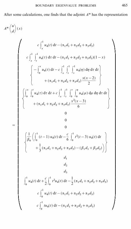
File: DISTL2 382958 . By:JB . Date:12:02:01 . Time:11:12 LOP8M. V8.B. Page 01:01Codes: 2122 Signs: 497 . Length: 45 pic 0 pts, 190 mm
After some calculations, one finds that the adjoint A* has the representation
A* \ud+ (x)
=
c |1
xu4(t) dt&(:1 d1+:2d2+:3 d3)
c |1
x|
1
tu4({) d{ dt&(:1d1+:2d2+:3d3)(1&x)
{&|
x
0u4(t) dt&c |
1
x|
1
t|
1
{u4(') d' d{ dt
=+(:1d1+:2d2+:3d3)x(x&2)
2
{|x
0|
t
0u4({) d{ dt+c |
1
x|
1
t|
{
0|
'
0u4(+) d+ d' d{ dt
=+(:1d1+:2 d2+:3 d3)x2(x&3)
6
0
0
0
{1
;0 \|1
0(t&1) u4(t) dt&
c6 |
1
0t2(t&3) u4(t) dt
=+13
(:1d1+:2d2+:3d3)&(;1 d1+;2d2)+d1
d2
d3
|1
0u4(t) dt+
c2 |
1
0t2u4(t) dt&
12
(:1 d1+:2d2+:3 d3)
c |1
0u4(t) dt&(:1 d1+:2 d2+:3 d3)
c |1
0tu4(t) dt&(:1d1+:2 d2+:3d3)
465BOUNDARY EIGENVALUE PROBLEMS

File: DISTL2 382959 . By:JB . Date:12:02:01 . Time:11:12 LOP8M. V8.B. Page 01:01Codes: 2038 Signs: 723 . Length: 45 pic 0 pts, 190 mm
for x # [0, 1] where u=(ui)7i=1 # (L2(0, 1))7, d=(di)
7i=1 # C7. It is not
difficult to see that
Ker A*={\ud+ # (L2(0, 1))7_C7 : d1=d2=d3=0, u4 #0= .
Using that (u, d )t # Ker(A*)2 if and only if A*(u, d )t # Ker A*, one obtainsthat
Ker(A*)2={\ud+ # (L2(0, 1))7_C7 : d1=d2=0,
u (2)4 +cu4=0, u4(0)=:3d3 , u$4(0)=&:3d3= .
It is more involved to show that
Ker(A*)3={\ud+ # (L2(0, 1))7_C7 : d1=0,
13
u$4(1)&12
u4(1)+13
(:2d2+:3 d3)&;2 d2=0,
u (4)4 +2cu (2)
4 +c2u4=0,
u4(0)=(:2d2+:3d3)&c:3 d2 ,
u$4(0)=&(:2d2+:3 d3)+c:3d2 ,
u (2)4 (0)=&c(:2d2+:3d3)+c2:3 d2 ,
u (3)4 (0)=c(:2d2+:3d3)&c2:3 d2= .
Calculating the explicit formula for u4 , we finally obtain that fork=3, 4, ...,
Ker(A*)k=Ker(A*)3
={\ud+ # (L2(0, 1))7_C7 : d1=0,
u4(x)=&(:2d2+:3d3&c:3d2) w(x),
13
u$4(1)&12
u4(1)+13
(:2d2+:3d3)&;2d2=0= ,
466 CHRISTIANE TRETTER

File: DISTL2 382960 . By:JB . Date:12:02:01 . Time:11:12 LOP8M. V8.B. Page 01:01Codes: 3021 Signs: 1549 . Length: 45 pic 0 pts, 190 mm
where the function w is given by
w(x) :={1
- csin(- c x)&cos(- c x) if c{0,
x # [0, 1]. (6.13)
x&1 if c=0,
If c=0, the equation for d2 in Ker(A*)3 implies that d2=0, and henceKer(A*)3=Ker(A*)2; for c{0, however, it yields d2=k(:2 , :3 , ;2 , c) d3
where k(:2 , :3 , ;2 , c) is a nonzero constant depending on :2 , :3 , ;2 , andc, and hence Ker(A*)3{Ker(A*)2.
By the definition in (3.1), y # V3 if and only if T0 y = Ker(A*)3 which is inturn equivalent to the following 11 conditions for y=( yi)
7i=1 # (W 1
2(0, 1))7:
y$1#y2 , y$2#y3 , y$3#y4 , y$5#0, y$6#0, y$7#0,
&((:2&c:3) k(:2 , :3 , ;2 , c)+:3) |1
0y$4(x) w(x) dx
+k(:2 , :3 , ;2 , c)( y5(0)+:1y1(1)+;1y4(1))
+ y6(0)+:2 y1(1)+;2y4(1)=0,
y7(0)+:3 y1(1)=0, y3(1)=0, y1(0)=0, y2(0)=0,
with w given by (6.3) and where we have set k(:2 , :3 , ;2 , c)=0 for c=0.Now Qn=Q4 is the projection of (W 1
2(0, 1))7 onto the first 4 components.Therefore,
Q4V3=[( yi)4i=1 # (W 1
2(0, 1))4 : y$1#y2 , y$2#y3 , y$3#y4 ,
y1(0)=0, y2(0)=0, y3(1)=0].
This implies that
V43=S&1(Q4V3)=[' # W 4
2(0, 1) : '(0)=0, '$(0)=0, '(2)(1)=0].
The representations of the spaces V l3 for l=0, 1, 2, 3 follow by taking the
closure of V43 in W l
2(0, 1) (see (3.4)). K
6.4. Minimality of the Eigenfunctions and Associated Functions
The eigenfunctions and associated functions of boundary eigenvalueproblems for differential equations N'=*P', even with *-independentboundary conditions, are not necessarily minimal in L2(0, 1) or higherorder Sobolev spaces. If we apply the minimality theorem of Section 4 tothe boundary eigenvalue problem of the elastic bar considered in thischapter, we obtain the subsequent result.
467BOUNDARY EIGENVALUE PROBLEMS

File: DISTL2 382961 . By:JB . Date:12:02:01 . Time:11:12 LOP8M. V8.B. Page 01:01Codes: 2858 Signs: 1845 . Length: 45 pic 0 pts, 190 mm
Theorem 6.4. Each canonical system of eigenfunctions and associatedfunctions of the boundary eigenvalue problem (6.1), (6.2) is minimal withdefect �3 in W l
2(0, 1) for l=2, 3, 4. That is, one has to remove at most 3elements such that the remaining system is minimal in W l
2(0, 1) while preservingcompleteness in V l
3 for l=2, 3, 4.
Proof. The assertion follows directly from Theorem 4.1 since n=3. K
6.5. Riesz Basis Properties
The eigenfunctions and associated functions of a non-self-adjoint boundaryeigenvalue problem as considered here are non-orthogonal. For a non-orthogonal system, however, completeness and minimality do not implythat it is also a basis. For it may happen that the respective Fourier seriesdoes not converge. Applying the basis theorem of Section 5, we obtain thatconvergence indeed takes place for the boundary eigenvalue problem of theelastic bar considered here.
Theorem 6.5. Each canonical system of eigenfunctions and associatedfunctions of the boundary eigenvalue problem (6.1), (6.2) is a Riesz basis withdefect �3 in the spaces
V23=[' # W 2
2(0, 1) : '(0)=0, '$(0)=0],
V33=[' # W 3
2(0, 1) : '(0)=0, '$(0)=0, '"(1)=0],
V43=[' # W 4
2(0, 1) : '(0)=0, '$(0)=0, '"(1)=0].
That is, for each function f # V l3 the Fourier series with respect to this
canonical system of eigenfunctions and associated functions converges in thenorm of W l
2(0, 1) for l=2, 3, 4.
Proof. Obviously, the (constant) coefficients of (6.1), (6.2) fulfill theconditions of Theorem 5.7. Furthermore, the problem is Stone-regular oforder }0=0 due to Theorem 6.1. In the proof of the latter it has also beenshown that q0=7. From the linearization stated in Theorem 6.2 one readsoff that the orders l1 , ..., l7 introduced in Definition 5.1 are given by
l1=3, l2=3, l3=3, l4=0, l5=2, l6=0, l7=1.
Hence
l(2)=max[l&1+l&2
+2(3&k) : [&1 , ..., &k]/[1, 2, 3],
[&k+1 , ..., &2]/[4, 5, 6, 7], k=0, 1, 2]
=9,
468 CHRISTIANE TRETTER
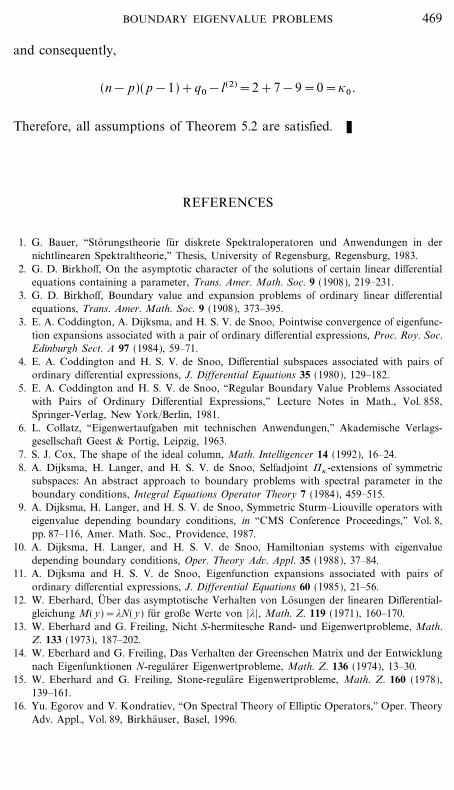
File: DISTL2 382962 . By:JB . Date:12:02:01 . Time:11:12 LOP8M. V8.B. Page 01:01Codes: 7831 Signs: 2889 . Length: 45 pic 0 pts, 190 mm
and consequently,
(n& p)( p&1)+q0&l(2)=2+7&9=0=}0 .
Therefore, all assumptions of Theorem 5.2 are satisfied. K
REFERENCES
1. G. Bauer, ``Sto� rungstheorie fu� r diskrete Spektraloperatoren und Anwendungen in dernichtlinearen Spektraltheorie,'' Thesis, University of Regensburg, Regensburg, 1983.
2. G. D. Birkhoff, On the asymptotic character of the solutions of certain linear differentialequations containing a parameter, Trans. Amer. Math. Soc. 9 (1908), 219�231.
3. G. D. Birkhoff, Boundary value and expansion problems of ordinary linear differentialequations, Trans. Amer. Math. Soc. 9 (1908), 373�395.
3. E. A. Coddington, A. Dijksma, and H. S. V. de Snoo, Pointwise convergence of eigenfunc-tion expansions associated with a pair of ordinary differential expressions, Proc. Roy. Soc.Edinburgh Sect. A 97 (1984), 59�71.
4. E. A. Coddington and H. S. V. de Snoo, Differential subspaces associated with pairs ofordinary differential expressions, J. Differential Equations 35 (1980), 129�182.
5. E. A. Coddington and H. S. V. de Snoo, ``Regular Boundary Value Problems Associatedwith Pairs of Ordinary Differential Expressions,'' Lecture Notes in Math., Vol. 858,Springer-Verlag, New York�Berlin, 1981.
6. L. Collatz, ``Eigenwertaufgaben mit technischen Anwendungen,'' Akademische Verlags-gesellschaft Geest 6 Portig, Leipzig, 1963.
7. S. J. Cox, The shape of the ideal column, Math. Intelligencer 14 (1992), 16�24.8. A. Dijksma, H. Langer, and H. S. V. de Snoo, Selfadjoint 6} -extensions of symmetric
subspaces: An abstract approach to boundary problems with spectral parameter in theboundary conditions, Integral Equations Operator Theory 7 (1984), 459�515.
9. A. Dijksma, H. Langer, and H. S. V. de Snoo, Symmetric Sturm�Liouville operators witheigenvalue depending boundary conditions, in ``CMS Conference Proceedings,'' Vol. 8,pp. 87�116, Amer. Math. Soc., Providence, 1987.
10. A. Dijksma, H. Langer, and H. S. V. de Snoo, Hamiltonian systems with eigenvaluedepending boundary conditions, Oper. Theory Adv. Appl. 35 (1988), 37�84.
11. A. Dijksma and H. S. V. de Snoo, Eigenfunction expansions associated with pairs ofordinary differential expressions, J. Differential Equations 60 (1985), 21�56.
12. W. Eberhard, U� ber das asymptotische Verhalten von Lo� sungen der linearen Differential-gleichung M( y)=*N( y) fu� r gro?e Werte von |*|, Math. Z. 119 (1971), 160�170.
13. W. Eberhard and G. Freiling, Nicht S-hermitesche Rand- und Eigenwertprobleme, Math.Z. 133 (1973), 187�202.
14. W. Eberhard and G. Freiling, Das Verhalten der Greenschen Matrix und der Entwicklungnach Eigenfunktionen N-regula� rer Eigenwertprobleme, Math. Z. 136 (1974), 13�30.
15. W. Eberhard and G. Freiling, Stone-regula� re Eigenwertprobleme, Math. Z. 160 (1978),139�161.
16. Yu. Egorov and V. Kondratiev, ``On Spectral Theory of Elliptic Operators,'' Oper. TheoryAdv. Appl., Vol. 89, Birkha� user, Basel, 1996.
469BOUNDARY EIGENVALUE PROBLEMS
File: DISTL2 382963 . By:JB . Date:12:02:01 . Time:11:12 LOP8M. V8.B. Page 01:01Codes: 9391 Signs: 3561 . Length: 45 pic 0 pts, 190 mm
17. W. N. Everitt, On certain regular ordinary differential expressions and related differentialoperators, in ``Proc. of the Int. Conf. on Spectral Theory of Differential Operators,University of Alabama Birmingham, 1981,'' Mathematical Studies, Vol. 55, pp. 115�167,North-Holland, Amsterdam, 1981.
18. C. T. Fulton, Two-point boundary value problems with eigenvalue parameter containedin the boundary conditions, Proc. Roy. Soc. Edinburgh Sect. A 77 (1977), 293�308.
19. H. Gail, ``Randeigenwertprobleme mit Randbedingungen, die polynomial vom Spektral-parameter abha� ngen,'' Thesis, University of Regensburg, Regensburg, 1996.
20. C. Gheorgiu and I. S. Pop, A modified Chebyshev-tau method for a hydrodynamicstability problem, in ``Approximization and Optimization, Proceedings of the Interna-tional Conference on Approximization and Optimization, Romania��ICAOR,'' Vol. II,pp. 119�126, Transsilvania Press, 1997.
21. I. C. Gohberg, S. Goldberg, and M. A. Kaashoek, ``Classes of Linear Operators, Vol. I,''Oper. Theory: Adv. Appl., Vol. 49, Birkha� user, Basel, 1990.
22. G. Heisecke, Rand-Eigenwertprobleme N( y)=*P( y) bei *-abha� ngigen Randbedingungen,Mitt. Math. Sem. Giessen 145 (1980), 1�74.
23. E. Kamke, U� ber die definiten selbstadjungierten Eigenwertaufgaben bei gewo� hnlichenDifferentialgleichungen, I�IV, Math. Z. 45 (1939), 759�787; Math. Z. 46 (1940), 231�250;Math. Z. 46 (1940), 251�286; Math. Z. 48 (1942�1943), 67�100.
24. E. Kamke, ``Differentialgleichungen I,'' Akademische Verlagsgesellschaft Geest 6 Portig,Leipzig, 1969.
25. F.-J. Kaufmann, Abgeleitete Birkhoff�Reihen bei Randeigenwertproblemen zu N( y)=*P( y) mit *-abha� ngigen Randbedingungen, Mitt. Math. Sem. Giessen 190 (1989).
26. J. L. Lagrange, ``Sur la figure des colonnes,'' Oeuvres de Lagrange, Gauthier�Villars,Paris, 1867.
27. P. Lancaster, A. A. Shkalikov, and Q. Ye, Strongly definitizable pencils in Hilbert space,Integral Equations Operator Theory 17 (1993), 338�360.
28. H. Langer, R. Mennicken, and C. Tretter, A selfadjoint linear pencil Q&*P of ordinarydifferential operators, Methods Funct. Anal. Topology 2, No. 1 (1996), 38�54.
29. H. Langer and C. Tretter, Spectral properties of the Orr�Sommerfeld problem, Proc. Roy.Soc. Edinburgh Sect. A 127, No. 6 (1997), 1245�1261.
30. R. E. Langer, The expansion problem in the theory of ordinary linear differentialequations of the second order, Trans. Amer. Math. Soc. 31 (1929), 868�906.
31. R. E. Langer, On the zeros of exponential sums and integrals, Bull. Amer. Math. Soc. 37(1931), 213�239.
32. R. E. Langer, The boundary problem of an ordinary linear differential system in thecomplex domain, Trans. Amer. Math. Soc. 46 (1939), 151�190.
33. C. C. Lin, ``The Theory of Hydrodynamic Stability,'' Cambridge Univ. Press, Cambridge,UK, 1955.
34. A. S. Markus, ``Introduction to the Theory of Polynomial Operator Pencils,'' Transl.Math. Monogr., Vol. 71, Amer. Math. Soc., Providence, 1988.
35. R. Mennicken and M. Mo� ller, ``Boundary Eigenvalue Problems,'' Notas A� lgebra Ana� l.,Vol. 14, Bahia Blanca, 1986.
36. R. Mennicken and M. Mo� ller, ``Nonselfadjoint Boundary Eigenvalue Problems,'' Elsevier,North�Holland, Amsterdam, in preparation.
37. R. Mennicken and H. D. Niessen, (S, S� )-adjungierte Randwertoperatoren, Math. Nachr.44 (1970), 259�284.
38. W. E. Milne, On certain asymptotic expressions in the theory of linear differentialequations, Proc. Nat. Acad. Sci. U.S.A. 2 (1916), 543�545.
39. W. E. Milne, Note on asymptotic expressions in the theory of linear differential equations,Bull. Amer. Math. Soc. 23 (1917), 166�169.
470 CHRISTIANE TRETTER
File: DISTL2 382964 . By:JB . Date:12:02:01 . Time:11:12 LOP8M. V8.B. Page 01:01Codes: 7673 Signs: 2994 . Length: 45 pic 0 pts, 190 mm
40. M. A. Naimark, ``Linear Differential Operators I, II,'' Ungar, New York, 1967.41. P. Schmidt, ``Zur Spektraltheorie einiger Schwingungsprobleme der Technischen
Mechanik,'' Diploma thesis, University of Regensburg, Regensburg, 1990.42. F. W. Scha� fke and A. Schneider, S-hermitesche Rand-Eigenwertprobleme, I�III, Math.
Ann. 162 (1965), 9�26; Math. Ann. 165 (1966), 235�260; Math. Ann. 177 (1968), 67�94.43. A. Schneider, Zur Einordnung selbstadjungierter Rand-Eigenwertprobleme bei gewo� hnlichen
Differentialgleichungen in die Theorie S-hermitescher Rand-Eigenwertprobleme, Math.Ann. 178 (1968), 277�294.
44. A. A. Shkalikov, Boundary value problems for ordinary differential equations with aparameter in the boundary conditions, J. Soviet Math. 33, No. 6 (1986), 1311�1342.
45. A. A. Shkalikov and C. Tretter, Kamke problems: Properties of the eigenfunctions, Math.Nachr. 170 (1994), 251�275.
46. A. A. Shkalikov and C. Tretter, Spectral analysis for linear pencils N&*P of ordinarydifferential operators, Math. Nachr. 179 (1996), 275�305.
47. M. H. Stone, An unusual type of expansion problem, Trans. Amer. Math. Soc. 26 (1924),335�355.
48. M. H. Stone, A comparison of the series of Fourier and Birkhoff, Trans. Amer. Math. Soc.28 (1926), 695�761.
49. M. H. Stone, The expansion problems associated with regular differential systems of thesecond order, Trans. Amer. Math. Soc. 29 (1927), 826�844.
50. J. D. Tamarkin, ``Some General Problems of the Theory of Ordinary Differential Equa-tions and Expansion of an Arbitrary Function in Series of Fundamental Functions,''Thesis, Petrograd, 1917. [In Russian].
51. J. D. Tamarkin, Some general problems of the theory of ordinary differential equationsand expansion of an arbitrary function in series of fundamental functions, Math. Z. 27(1928), 1�54.
52. C. Tretter, ``On *-Nonlinear Boundary Eigenvalue Problems,'' Mathematical Research,Vol. 71, Akademie Verlag, Berlin, 1993.
53. C. Tretter, Nonselfadjoint spectral problems for linear pencils N&*P of ordinary differentialoperators with *-linear boundary conditions: Completeness results, Integral EquationsOperator Theory 26 (1996), 222�248.
54. C. Tretter, On buckling problems, Z. Angew. Math. Mech. 80 (2000), 633�639.55. C. Tretter, A linearization for a class of *-nonlinear boundary eigenvalue problems,
J. Math. Anal. Appl. 247 (2000), 331�355.56. C. Tretter, Linear operator pencils A&*B with discrete spectrum, Integral Equations
Operator Theory 37 (2000), 357�373.57. C. Tretter, Spectral problems for systems of differential equations y$+A0 y=*A1 y with
*-polynomial boundary conditions, Math. Nachr. 214 (2000), 129�172.58. E. Wagenfu� hrer, On the linearization of a differential equation with a polynomial
parameter dependence, unpublished manuscript, Regensburg, 1976.59. E. Zeidler, ``Nonlinear Functional Analysis and Its Applications. Vol. 2A. Linear
Monotone Operators. Vol. 2B. Nonlinear Monotone Operators,'' Springer-Verlag, NewYork, 1986.
471BOUNDARY EIGENVALUE PROBLEMS