bounds on range and range rate for optical tracking of...

Distribution statement

Bounds on Range and Range Rate for Optical Tracking of Satellites

Paul W. Schumacher, Jr. Air Force Research Laboratory

ABSTRACT

We propose a type of admissible-region analysis for track initiation in multi-satellite problems when angles are the primary observable. For a specified rectangular partition in the space of orbital elements, we present explicit upper and lower bounds for the values of range and range rate that will lead to initial orbit hypotheses (data association hypotheses) associated with that partition. These bounds allow us to parallelize the generation of candidate orbits, because each element-space partition can be handled independently of the others. Measured or derived angle rates provide additional bounds on range and range rate, also permitting the same parallelism.

INTRODUCTION The advent of high-sensitivity, high-capacity optical sensors for space surveillance presents us with interesting and challenging tracking problems. Accounting for the origin of every detection made by such systems is generally agreed to belong to the “most difficult” category of tracking problems. Especially in the early phases of the tracking scenario, when a catalog of space objects is being compiled, or when many new objects appear in space because of on-orbit explosion or collision, one faces a combinatorially large number of tracking hypotheses to evaluate. The number of hypotheses is reduced to a more feasible number if observations close together in time can, with high confidence, be associated by the sensor into extended tracks on single objects. Most current space surveillance techniques are predicated on the sensor systems’ ability to form such tracks reliably. However, the required operational tempo of space surveillance, the very large number of objects in Earth orbit and the difficulties of detecting dim, fast-moving objects at long ranges mean that individual sensor track reports are often inadequate for computing initial orbit hypotheses. In fact, this situation can occur with optical sensors even when the probability of detection is high. For example, the arc of orbit that has been observed may be too short or may have been sampled too sparsely to allow well-conditioned, usable orbit estimates from single tracks. In that case, one has no choice but to solve a data association problem involving an unknown number of objects and many widely spaced observations of uncertain origin. In the present paper, we are motivated by this more difficult aspect of the satellite cataloging problem. However, the results of this analysis may find use in a variety of less stressing tracking applications.

2

Assume that we have a pair of line-of-sight unit vectors 𝐮1 and 𝐮2 , measured at time 𝑡1 at station position 𝐑1 and time 𝑡2 at station position 𝐑2, respectively. Assume, without loss of generality, that 𝑡2 > 𝑡1. We want to test the hypothesis that these two observations are associated with the same space object. To this end, we attach a set of hypothetical range values, �𝜌1,𝑚 ,𝑚 = 1,2, … � and �𝜌2,𝑛 ,𝑛 = 1,2, … � respectively, to each of these measured unit vectors and then generate candidate orbits by solving Lambert’s problem for each of the pair-wise combinations of hypothetical orbital position vectors 𝐫1,𝑚 and 𝐫2,𝑛. With a large dataset of measured line-of-sight unit vectors, we can, in principle, consider all possible pairs of observations and solve the family of Lambert problems for each pair. Then each hypothetical orbit from the solution of Lambert’s problem is a data association hypothesis that must be either confirmed or eliminated through comparisons with other observational data. This approach allows us to make use of an already proven method (the Search and Determine algorithm and software, SAD) that was designed for generating and testing data association hypotheses for position-type observations typical of radar sensors [9,10,11]. Given enough range hypotheses for each observed line of sight, we are guaranteed to generate a viable candidate orbit for every object that has been observed at two or more distinct times. However, the Cartesian product of the set of range values for each observed line of sight with the sets of range values from every other line of sight implies a possibly prohibitive number of Lambert solutions to generate and check. The computational complexity for generating hypothetical orbits on this approach is quadratic in the number of observed lines of sight and also quadratic in the number of range hypotheses that we attach to the observations. How should we limit the number of range hypotheses to make the total number of candidate orbits manageable while also generating candidates that are likely to correspond to real orbits of interest? For example, we may be most interested in generating candidate orbits near the geosynchronous equatorial orbital (GEO) belt. Let us seek to generate hypotheses for orbits that lie only in a bounded region of semimajor axis 𝑎 , eccentricity 𝑒 , inclination 𝐼 and right

3

ascension of the ascending node Ω , namely, within a partition specified by the intervals [𝑎MIN ,𝑎MAX] , [𝑒MIN , 𝑒MAX] , [𝐼MIN , 𝐼MAX] and [ΩMIN ,ΩMAX] . (For the purposes of this discussion, we leave the other orbital elements unconstrained. It will turn out that these four elements constrain the possible values of range in simple ways without our having any recourse to angle rate information.) Then, to the extent that we can restrict the generation of hypothetical orbits to a specified partition of the space of orbital elements, we have parallelized the task of building a catalog of objects detected within that partition. The reason is that any partition of the space of orbital elements, including the whole space itself, can be sub-divided into smaller partitions, and each sub-partition can be handled independently. In the approach outlined here, all the observations would have to be considered for each sub-partition of the space of orbit elements. However, by constructing upper and lower bounds on range for each sub-partition of the element space, we limit the number of range hypotheses that have to be considered for each sub-partition. This approach allows us to consider a manageable number of range hypotheses for each sub-partition before we generate candidate orbits, simply by making the sub-partitions small enough, so that the overall computation is feasible. Our emphasis on generating candidate orbits with a Lambert-based approach is not merely a matter of convenience in extending an existing method such as SAD. Certainly, the bounds on range and range rate that we present here could be used in a variety of ways with other angles-based initial orbit determination methods. All the traditional methods of angles-only orbit determination, plus the modern methods of Gooding, Mortari and Karimi, and others [6,7,8,19], rely on solving for the range by either a root-finding method or an optimization method. Such algorithms can always be made to work more reliably when rigorous upper and lower bounds on the unknown quantity are available. However, one encounters at least three difficulties in trying to apply direct angles-only methods to a large, multiple-target catalog-building scenario. First, although the range bounds presented here allow one to reject candidate solutions based on range, with a direct angles-only method one still has to compute the range in terms of the observations in order to find out if it satisfies the bounds. This turns out to be most of the computation needed to produce the candidate orbits themselves. In the Lambert-based approach, the range bounds allow us to avoid most of the potential computation for the candidate orbits. Second, the direct angles-only methods do not scale to large problems as well as a Lambert-based method does. Given 𝑁observations of line of sight, not necessarily close together in time, the computational load of Lambert-based methods is proportional to 𝑁2, because two observations per data association hypothesis are needed. The “constant” of proportionality is itself quadratic in the number of range hypotheses that must be considered for each line of sight. However, as noted above, the latter number can be driven down to manageable size in each partition of the element space by making the partitions small. With traditional methods of angles-only initial orbit determination, including that of Gooding [6,7], one faces a computational load that is proportional to 𝑁3, because 3 observations must be associated together to compute the range and hence the candidate orbit. The methods developed by Mortari and Karimi are more robust than traditional methods, but these also require at least 3 observations per association hypothesis. In fact, the approach of Mortari and Karimi [19] works better with more observations per association hypothesis, but then one faces a computational load that scales like 𝑁4, 𝑁5, or even higher. In general, the computational complexity is polynomial in the number of

4

observations, with the polynomial degree equal to the number of observations per data association hypothesis. Of course, it is not clear in general which approach finally requires fewer processors to achieve a desired production rate of orbit solutions. Higher-degree scaling requires more processors on the traditional range-solution approach and smaller element partitions require more processors on the range-hypothesis approach. The choice may depend on the size and character of the dataset itself. Third, a Lambert-based method, ideally implemented, will produce a candidate orbit for every real object that has been observed at least twice. In comparison, a direct angles-based method, such as Gooding’s, will produce candidate orbits only for those real objects that have been observed at least 3 times. An 𝑁4 method will produce candidate orbits only for those real objects that have been observed at least 4 times, and so on. Hence, the Lambert-based method may do a more complete job of generating viable candidate orbits from real datasets, while scaling more favorably than the direct angles-based methods for large numbers of observations. We are seeking explicit bounds on range and possibly range rate that can be applied for each individual angle-based observation, or at most to pairs of angle-based observations. Even with the further restriction that hypothetical orbits be elliptical and Keplerian (which we accept) and even allowing the possibility that the observation may include angle rate values (which we will examine at length), it may not be obvious that efficient bounds having these properties can be obtained. Exact bounds would have to be based on some admissible-region analysis of the type developed by Milani, Tommei, Scheeres, Maruskin, Fujimoto and others [12-18]. For example, denoting the gravitational parameter by 𝜇 , we write the first integrals of Keplerian motion as energy: 𝐸 = (�̇� ∙ �̇�) 2⁄ − 𝜇 ‖𝐫‖⁄ (i) angular momentum: 𝐡 = 𝐫 × �̇� (ii) Laplace vector: 𝜇𝐞 = �̇� × (𝐫 × �̇�) − 𝜇𝐫 ‖𝐫‖⁄ (iii) These can be evaluated with the vector triangle relation 𝐫 = 𝐑 + 𝜌𝐮 and its time derivative �̇� = �̇� + �̇�𝐮 + 𝜌�̇� for each observation. Then, for each observation, we can define admissible regions in the (𝜌, �̇�) plane for each partition in the space of elements by means of inequalities such as −𝜇 (2𝑎MIN)⁄ ≤ 𝐸 ≤ −𝜇 (2𝑎MAX)⁄ (iv) cos𝐼MAX ≤ (𝐡 ‖𝐡‖⁄ ) ∙ 𝐤 ≤ cos𝐼MIN (v) 𝑒MIN ≤ ‖𝐞‖ ≤ 𝑒MAX (vi) Here 𝐤 is the north polar unit vector in the Earth-centered inertial frame. For each observation, the values of range and range rate that satisfy these inequalities will result in orbits that lie only within the given partition of the space of elements. DeMars and Jah [2] have shown what the admissible regions look like for partitions of semimajor axis and eccentricity by a numerical treatment of the above inequalities. Maruskin, et al. [3], have shown how the admissible regions evolve in time and how the overlap of the admissible regions for different observations can help solve the data association problem. However, even though expressions (i) through (vi) can be reduced to polynomial forms in range and range rate, each relation is coupled in both variables and the polynomial degree is high, preventing us from obtaining explicit expressions for range and range rate in terms of the given data. Moreover, the usual admissible-region analysis leads

5

nowhere if angle rates are not available. For example, the track-initiation method of DeMars, et al.[1], involving multiple hypotheses on range and range rate, requires both angle and angle rate values. In the present analysis, we take a geometric and kinematic approach that does lead to explicit upper and lower bounds on the possible values of range for each observation or pair of observations, given only angle data at discrete times. In fact, we find several inequalities that must be satisfied simultaneously, and we can take the most restrictive superposition of the different bounds as our working result. In case angle rates are available, we can obtain explicit upper and lower bounds on range rate, as well as additional bounds on range. It may happen that, for a given observation, there are no values of the range or range rate that lead to orbits within the given element-space partition, so that the observation can be eliminated from further consideration. We obtain explicit conditions for the existence of possible values of range and range rate, in terms of the observation itself. The price for obtaining explicit bounds on range and range rate is that the bounds are not exact but somewhat conservative. Although every orbit within the element-space partition corresponds to values of range and range rate that lie within the bounds given here, some values of range or range rate that satisfy the bounds may lead to orbits that lie outside the given partition. This situation represents inefficiency in the parallelization of building the catalog: nearly the same candidate orbits near the boundaries of the element-space partitions may be generated in both of the adjacent partitions, if the range or range rate hypotheses are planted densely enough. On the other hand, no candidate orbits within the given element-space partitions will be missed because of the bounds given here. The extent and cost of the inefficient duplication of candidate orbits will depend on the particular datasets and element partitions of interest, and may require further study. In practice, of course, within any element partition, any of these extra orbit hypotheses can be either kept or discarded. If they are kept, one would have, at most, a bookkeeping problem of transferring the extra orbits to the correct element partition. The trade-off in this case is that merely moving data between processors always takes time. BOUNDS ON RANGE IMPLIED BY ANGLE VALUES Here we present bounds on range that must hold for each observed line of sight. Assuming that all orbits of interest are elliptical, require that the orbital radii lie between the maximum specified apogee and the minimum specified perigee: 𝑎MIN (1− 𝑒MAX) ≤ ‖𝐫‖ ≤ 𝑎MAX(1 + 𝑒MAX) (1) The values of range that correspond to these limits on orbital radius can be found explicitly using the vector triangle relationship 𝐫 = 𝐑 + 𝜌𝐮 . Squaring terms to remove the radical, we have 𝑎MIN2 (1 − 𝑒MAX)2 ≤ 𝐑 ∙ 𝐑 + 2(𝐑 ∙ 𝐮)𝜌 + 𝜌2 ≤ 𝑎𝑀𝐴𝑋2 (1 + 𝑒MAX)2 (2) Consider the perigee and apogee cases separately. For the perigee case, we require the orbital radius to be no smaller than the smallest allowable perigee radius:

6

𝑎MIN2 (1 − 𝑒MAX)2 ≤ 𝐑 ∙ 𝐑 + 2(𝐑 ∙ 𝐮)𝜌 + 𝜌2 (3) 𝜌2 + 2(𝐑 ∙ 𝐮)𝜌 − [𝑎MIN2 (1 − 𝑒MAX)2 − 𝐑 ∙ 𝐑] ≥ 0 (4) The roots of this quadratic are:

𝜌 = −(𝐑 ∙ 𝐮) ± �(𝐑 ∙ 𝐮)2 + [𝑎MIN2 (1− 𝑒MAX)2 − 𝐑 ∙ 𝐑] (5)

We will have real roots if and only if the argument of the square root is non-negative: 𝑎MIN2 (1 − 𝑒MAX)2 ≥ 𝐑 ∙ [𝐑 − (𝐑 ∙ 𝐮)𝐮] (6) If no real roots of the quadratic expression (4) exist, then we can immediately discard the current observation and form no hypotheses with it. The reason is that no value of the range will be found for this observation, which is consistent with the specified intervals of the orbital elements. Descartes’ rule of signs tells us the number of positive real roots. If the third coefficient in the quadratic form (4) is negative, that is, if 𝑎MIN2 (1− 𝑒MAX)2 > 𝐑 ∙ 𝐑 , then, regardless of the sign of the second coefficient 2(𝐑 ∙ 𝐮), we will have one positive real root and necessarily also one negative root. Because the quadratic is concave-up, the inequality is satisfied to the left of the negative root and to the right of the positive root. We can ignore the negative root and all values to the left of it, because we require a priori that range values to be non-negative. What remains is a positive lower limit on the possible values of range:

𝜌 ≥ −(𝐑 ∙ 𝐮) + �(𝐑 ∙ 𝐮)2 + [𝑎MIN2 (1− 𝑒MAX)2 − 𝐑 ∙ 𝐑] (7)

It is worth noting that, for Earth-bound stations, the third coefficient of (4) will essentially always be negative because the inequality 𝑎MIN2 (1− 𝑒MAX)2 > 𝐑 ∙ 𝐑 is approximately the condition that the minimum allowable perigee radius be larger than the Earth radius. Moreover, the second coefficient 2(𝐑 ∙ 𝐮) will essentially always be positive because observations have to be taken above the local horizontal plane at some positive local elevation angle. For space-based observing stations, it is possible that neither of these circumstances would be true: the station’s orbital position may be higher than the minimum specified perigee radius, or observations may be taken at negative local elevation angles, or both. If the third coefficient in (4) is positive, that is, if 𝑎MIN2 (1 − 𝑒MAX)2 < 𝐑 ∙ 𝐑 , then the quadratic will have either no positive real roots or two positive real roots, depending on the sign of the second coefficient. This is the possibility just mentioned for space-based stations, although we do not expect this possibility for Earth-bound stations unless we are interested in orbits with perigee radii less than the Earth radius. If, furthermore, the second coefficient in (4) is positive, that is, if (𝐑 ∙ 𝐮) > 0 , then we have no positive real roots, but only a pair of negative roots. Because the quadratic is concave-up, the inequality (4) is satisfied to the left of the more negative root and to the right of the less negative root. However, since we require a priori that

7

range values be non-negative, we are left merely with the condition that 𝜌 ≥ 0 . If the second coefficient is negative, that is, (𝐑 ∙ 𝐮) < 0 , meaning that the observation is taken at negative local elevation angle, then the quadratic will have two positive real roots. Because the quadratic is concave-up, the inequality (4) will be satisfied to the left of the smaller root, that is, between 𝜌 = 0 and the smaller root, and also to the right of the larger root. In this case, we have two disjoint intervals of range, one finite and one semi-infinite, over which range hypotheses will satisfy the perigee constraint:

0 ≤ 𝜌 ≤ −(𝐑 ∙ 𝐮) −�(𝐑 ∙ 𝐮)2 + [𝑎MIN2 (1− 𝑒MAX)2 − 𝐑 ∙ 𝐑] (8)

𝜌 ≥ −(𝐑 ∙ 𝐮) + �(𝐑 ∙ 𝐮)2 + [𝑎MIN2 (1 − 𝑒MAX)2 − 𝐑 ∙ 𝐑] (9)

Now we consider the apogee case and seek to derive results that are analogous to those above. The apogee case will provide us with conditions on values of the range that are complementary to those of the perigee case. Since both sets of conditions must be satisfied simultaneously, we can take the most restrictive superposition of all conditions on range to define the set of values over which we must form range hypotheses. For the apogee case, we have from the inequality (2) that the orbital radius must be no larger than the maximum allowable apogee radius: 𝐑 ∙ 𝐑 + 2(𝐑 ∙ 𝐮)𝜌 + 𝜌2 ≤ 𝑎𝑀𝐴𝑋2 (1 + 𝑒MAX)2 (10) 𝜌2 + 2(𝐑 ∙ 𝐮)𝜌 − [𝑎MAX2 (1 + 𝑒MAX)2 − 𝐑 ∙ 𝐑] ≤ 0 (11) The roots are:

𝜌 = −(𝐑 ∙ 𝐮) ± �(𝐑 ∙ 𝐮)2 + [𝑎MAX2 (1 + 𝑒MAX)2 − 𝐑 ∙ 𝐑] (12)

We will have real roots if and only if the argument of the square root is non-negative: 𝑎MAX2 (1 + 𝑒MAX)2 ≥ 𝐑 ∙ [𝐑 − (𝐑 ∙ 𝐮)𝐮] (13) If no real roots exist, then we can immediately discard the observation and form no hypotheses with it. The reason is that no value of the range will be found for this observation, which is also consistent with the specified intervals of the orbital elements. Assuming that we have real roots in equation (12), we use Descartes’ rule of signs to determine the number of positive real roots. If the third coefficient in the quadratic form (11) is negative, that is, if 𝑎MAX2 (1 + 𝑒MAX)2 > 𝐑 ∙ 𝐑 , then, regardless of the sign of the second coefficient 2(𝐑 ∙ 𝐮) , we will have one positive real root and necessarily also one negative root. Because the quadratic is concave-up, the inequality (11) is satisfied between the roots. Moreover, we require a priori that range values be non-negative, so we can say without loss of generality that the

8

inequality will be satisfied between 𝜌 = 0 and the positive real root. The result is that we have an upper bound on the possible values of range:

0 ≤ 𝜌 ≤ −(𝐑 ∙ 𝐮) + �(𝐑 ∙ 𝐮)2 + [𝑎MAX2 (1 + 𝑒MAX)2 − 𝐑 ∙ 𝐑] (14)

It is worth noting that, for Earth-bound stations, the third coefficient will essentially always be negative because the inequality 𝑎MAX2 (1 + 𝑒MAX)2 > 𝐑 ∙ 𝐑 is approximately the condition that the maximum allowable apogee radius be larger than the Earth radius. Moreover, the second coefficient 2(𝐑 ∙ 𝐮) will essentially always be positive because observations have to be taken above the local horizontal plane at some positive local elevation angle. For space-based observing stations, it is possible that neither of these circumstances would be true: the station’s orbital position may be above the maximum specified apogee radius, or observations may be taken at negative local elevation angles, or both. If the third coefficient in (11) is positive, that is, if 𝑎MAX2 (1 + 𝑒MAX)2 < 𝐑 ∙ 𝐑 , then the quadratic will have either no positive real roots or two positive real roots, depending on the sign of the second coefficient. This is the possibility just mentioned for space-based stations, although we do not expect this case for Earth-bound stations. If, furthermore, the second coefficient in (11) is positive, that is, if (𝐑 ∙ 𝐮) > 0 , then we have no positive real roots, but only a pair of negative roots. Because the quadratic is concave-up, the inequality (11) is satisfied between these roots. However, since we require a priori that range values be non-negative, we can discard this particular observation and form no range hypotheses for it. If the third coefficient in (11) is positive, but the second coefficient is negative, (𝐑 ∙ 𝐮) < 0 , meaning that the observation is taken at negative local elevation angle, then the quadratic will have two positive real roots. The quadratic is concave-up, so the inequality (11) will be satisfied between these two roots. In this case, we have a single finite interval of range over which range hypotheses will satisfy the apogee condition:

𝜌 ≥ −(𝐑 ∙ 𝐮) −�(𝐑 ∙ 𝐮)2 + [𝑎MAX2 (1 + 𝑒MAX)2 − 𝐑 ∙ 𝐑] (15)

𝜌 ≤ −(𝐑 ∙ 𝐮) + �(𝐑 ∙ 𝐮)2 + [𝑎MAX2 (1 + 𝑒MAX)2 − 𝐑 ∙ 𝐑]

(16)

The set of range values over which we may have to form hypotheses for the observation in question is given by the intersection of all of the above conditions, both perigee conditions and apogee conditions.

9

BOUNDS ON RANGE IMPLIED BY ANGLE VALUES, INCLINATION LIMITS AND NODAL LIMITS The above conditions are bounds on the possible values of range, which can be computed for each single observation. The fact that only single observations are involved is what allows us to find explicit bounds for each of the ranges before we form any range hypotheses. However, at least five additional restrictions on the allowable values of range can be deduced from relations that involve both of the ranges presented for a solution to Lambert’s problem. Although the nonlinearities in these relations prevent us from getting explicit inequalities like (7) – (9) and (14 – (16), nevertheless we can formulate additional conditions that 𝜌1 and 𝜌2 must satisfy. Checking these extra conditions for each range pair may keep us from having to produce some unnecessary and relatively expensive Lambert solutions. Using the vector triangle relation 𝐫 = 𝐑 + 𝜌𝐮 for each of the two lines of sight, compute the unit vector 𝐧 normal to the candidate orbital plane: 𝐧 = ± (𝐫1 × 𝐫2) ‖𝐫1 × 𝐫2‖⁄ (17) Here the ambiguous sign has to be resolved a priori. The choice depends on whether the angle between the position vectors (mod 2𝜋) exceeds 𝜋 or not, distinguishing between “long-way” and “short-way” orbits. With the sign chosen, the inclination is given unambiguously by cos 𝐼 = 𝐧 ∙ 𝐤 (18) The inclination of the candidate orbit lies in the specified interval [𝐼MIN , 𝐼MAX] provided that cos 𝐼 lies in the interval [cos 𝐼MAX , cos 𝐼MIN] . Hence we require that cos 𝐼MAX ≤ 𝐧 ∙ 𝐤 ≤ cos 𝐼MIN (19)

In the case of low-inclination intervals, it may be better to work in terms of sine inclination: sin 𝐼MIN ≤ �1 − (𝐧 ∙ 𝐤)2 ≤ sin 𝐼MAX (20)

In a similar way, we use the unit nodal vector to obtain conditions that the range pair must satisfy if the candidate orbit is to lie within a specified interval of right ascension of the ascending node, [ΩMIN ,ΩMAX] . In the Earth-centered inertial frame, we have (𝐤 × 𝐧) ‖𝐤 × 𝐧‖⁄ = (cosΩ , sinΩ , 0)T (21) so that, following standard logic for quadrant resolution, we require ΩMIN ≤ tan−1(sinΩ cosΩ⁄ ) ≤ ΩMAX (22) Of course, for important special cases like near-GEO orbits, it may be preferable to define element-space partitions in terms of nonsingular elements such as 𝑝 ≜ sin(𝐼 2⁄ ) cosΩ and

10

𝑞 ≜ sin(𝐼 2⁄ ) sinΩ . No special difficulty attaches to working in terms of these or any other elements related to the orbit plane. If any range-pair hypothesis (𝜌1 ,𝜌2) does not satisfy all of the above conditions, then that pair of values can be eliminated from further consideration without solving Lambert’s problem. The reason is that the geometry of the pair either will not allow an orbital inclination within its specified interval or will not allow a right ascension of the ascending node within its specified interval. Note that it is the pair of range values that is eliminated; either range value by itself may still lead to an acceptable hypothesis in combination with some other range value. BOUNDS ON RANGE IMPLIED BY ANGLE VALUES AND LAMBERT’S THEOREM Next, we can use three special solutions of Lambert's problem to restrict the ranges. The eccentricity of the orbit of least possible eccentricity that goes through a given pair of position vectors can be computed solely in terms of those position vectors. Call it 𝑒0 . Likewise, the semimajor axis of the orbit of least possible semimajor axis that goes through the pair of positions can be computed solely in terms of the position vectors. Call it 𝑎0 . Hence, for each hypothesized range pair (𝜌1 ,𝜌2) , we compute the corresponding position vectors and apply the following logic:

If 𝑎0 > 𝑎MAX , then reject the hypothesis pair without solving Lambert's problem, because the geometry is guaranteed to produce a larger semimajor axis than we have specified. If 𝑒0 > 𝑒MAX , then reject the hypothesis pair without solving Lambert's problem, because the geometry is guaranteed to produce a larger eccentricity than we have specified.

Of course, even for a (𝜌1 ,𝜌2) hypothesis that passes all of the above tests, the actual solution of Lambert's problem may still turn out to get rejected once we have computed the elements of the candidate orbit. The reason is that none of the conditions on range derived so far involves the minimum allowable eccentricity, 𝑒MIN . This fundamental feature of our problem raises the question of how well we can limit the generation of candidate orbits to lie within the given eccentricity interval. Let us assume that the hypothetical range pair is not rejected by the above criterion, so that 𝑒0 ≤ 𝑒MAX . Assume also that all of the range bounds and other conditions that depend on single observations have already been applied. Then we know that the Lambert solution for a pair of range hypotheses will not produce an orbit having eccentricity outside the interval [𝑒0 , 𝑒MAX] . If 𝑒MIN ≤ 𝑒0 , we have no difficulty: the candidate orbit will have an eccentricity within the given interval [𝑒MIN , 𝑒MAX] . However, if 𝑒0 < 𝑒MIN , then the eccentricity of the candidate orbit may or may not lie within the specified interval. The Lambert solution has to be generated and then either kept if the eccentricity is at least as large as 𝑒MIN or discarded if the candidate eccentricity turns out to be less than 𝑒MIN . This represents some inefficiency in the generation of candidate orbits, especially if those same candidate orbits were to be generated in the processing for other element-space partitions. (Naturally, one could simply move the discarded orbit to its correct element partition, though even that operation involves

11

computational overhead.) The extent of the overall inefficiency depends on the dataset and the actual element-space partitions being used, so we cannot draw general conclusions. It would be helpful at this point to have reasonably sharp bounds on the actual eccentricity in the Lambert problem without having to solve the whole problem. However, lacking that, we have no better recourse than to generate the candidate orbit. Overall, we do expect to be able to reduce the number of Lambert solutions that have to be generated, compared to the number required without the above checks involving 𝑎0 and 𝑒0. The formulas for 𝑎0 and 𝑒0 are well known, but the derivations are short and illuminating. An ellipse has the property that the sum of the radii from the two foci is constant. In particular, 𝑟1 + 𝑟1∗ = 2𝑎 and 𝑟2 + 𝑟2∗ = 2𝑎 (23)

where a superscript “*” denotes distance from the vacant focus. Therefore 𝑟1 + 𝑟2 + 𝑟1∗ + 𝑟2∗ = 4𝑎 (24) Hold the position vectors 𝐫1 and 𝐫2 fixed and vary the semimajor axis by moving the vacant focus throughout the plane of the orbit. The sum 𝑟1∗ + 𝑟2∗ reaches a global minimum when the vacant focus lies on the chord between 𝐫1 and 𝐫2 . In fact, the radii from the vacant focus obey the triangle inequality 𝑟1∗ + 𝑟2∗ ≥ ‖𝐫2 − 𝐫1‖ (25) We conclude that the minimum possible semimajor axis is given by 4𝑎0 = ‖𝐫1‖ + ‖𝐫2‖ + ‖𝐫2 − 𝐫1‖ (26) The eccentricity vector of minimum possible length can be obtained by considering the equation of the orbit:

𝑟1 =ℎ2 𝜇⁄

1 + 𝐞 ∙ 𝐫1 ‖𝐫1‖⁄ and 𝑟2 =ℎ2 𝜇⁄

1 + 𝐞 ∙ 𝐫2 ‖𝐫2‖⁄ (27)

Here 𝐞 is the eccentricity vector, ℎ is the angular momentum magnitude and 𝜇 is the gravitational constant. Then ℎ2 𝜇⁄ = 𝑟1 + 𝐞 ∙ 𝐫1 and ℎ2 𝜇⁄ = 𝑟2 + 𝐞 ∙ 𝐫2 (28) 𝑟1 + 𝐞 ∙ 𝐫1 = 𝑟2 + 𝐞 ∙ 𝐫2 (29) 𝐞 ∙ (𝐫2 − 𝐫1) = 𝑟1 − 𝑟2 (30) This shows that, for given position vectors in the Lambert problem, the locus of possible eccentricity vectors is a straight line normal to the chord vector in the orbital plane. The eccentricity vector varies with time of flight 𝑡2 − 𝑡1 in such a way that its projection on the chord vector 𝐜 = 𝐫2 − 𝐫1 is a constant, namely, the signed difference 𝑟1 − 𝑟2 . Therefore the

12

eccentricity 𝑒 = ‖𝐞‖ has no maximum value in the Lambert problem, but it does have a minimum value when 𝐞 is aligned with the chord vector. That minimal-length eccentricity vector can be written down directly in terms of the chord vector: 𝐞𝟎 = �𝐞 ∙

𝐜‖𝐜‖

�𝐜‖𝐜‖

= �𝐞 ∙𝐫2 − 𝐫1‖𝐫2 − 𝐫1‖

�𝐫2 − 𝐫1‖𝐫2 − 𝐫1‖

(31)

Using (30) to rewrite the scalar product, we have 𝐞𝟎 = �

𝑟1 − 𝑟2‖𝐫2 − 𝐫1‖

�𝐫2 − 𝐫1‖𝐫2 − 𝐫1‖

(32)

from which we get

𝑒02 = 𝐞𝟎 ∙ 𝐞𝟎 = �𝑟1 − 𝑟2‖𝐫2 − 𝐫1‖

�2

or 𝑒0 =|(‖𝐫1‖ − ‖𝐫2‖)|

‖𝐫2 − 𝐫1‖

(33)

Finally, we quote without proof a statement of Euler’s Theorem, a special case of Lambert’s Theorem, which expresses the time of flight ∆𝑡P between given position vectors on a parabolic (zero-energy) orbit:

∆𝑡P =43�𝑎0

3

𝜇(1 − 𝑠 𝜆3)

(33a)

Here the quantity 𝑠 is a signum function: 𝑠 = +1 for “short-way” trajectories and 𝑠 = −1 for “long-way” trajectories. The parameter 𝜆 is defined in terms of the position vectors:

0 ≤ 𝜆2 =‖𝐫1‖ + ‖𝐫2‖ − ‖𝐫2 − 𝐫1‖‖𝐫1‖ + ‖𝐫2‖ + ‖𝐫2 − 𝐫1‖

≤ 1 (33b)

Because, for given position vectors, the time of flight in Lambert’s problem is a monotonic decreasing function of the orbital energy, elliptic (negative-energy) orbits will always have a time of flight longer than the parabolic time, and hyperbolic (positive-energy) orbits will always have a time of flight shorter than the parabolic time. In our case, we can require that our observation pairs and range hypotheses always produce elliptic orbits: 𝑡2 − 𝑡1 > ∆𝑡P (33c) Combinations that do not satisfy this condition can be eliminated without generating a Lambert solution. Given an observation pair 𝐮1 and 𝐮2 , the previous formulas, and the associated logic, can be used to decide if a hypothetical pair of ranges should be used to generate a Lambert solution. Of course, whatever Lambert solutions are generated should be verified for compliance with the specified interval of eccentricity, because none of the conditions on range derived so far depends on the value of the minimum allowable eccentricity 𝑒MIN .

13

BOUNDS ON RANGE IMPLIED BY ANGLE AND ANGLE RATE VALUES In case the observations include, or allow us to derive, angle rates, we can deduce additional bounds on the possible values of range. Like the bounds derived above from perigee and apogee distances, these extra bounds will apply to single observations, where we now understand an observation to consist of the values �𝐑 , �̇� ,𝐮 , �̇� � at a known time. Differentiating the vector triangle relation 𝐫 = 𝐑 + 𝜌𝐮 , we get the orbital velocity at the observation time: �̇� = �̇� + �̇�𝐮 + 𝜌�̇� (34) The time derivative of the line-of-sight unit vector contains the angle rates in the following way. In terms of topocentric right ascension 𝛼 and declination 𝛿, the observed unit vector is

𝐮 = �cos 𝛿 cos𝛼cos 𝛿 sin𝛼

sin 𝛿�

(35)

Differentiating with respect to time, we get

�̇� = �−�̇� sin 𝛿 cos 𝛼−�̇� cos 𝛿 sin𝛼−�̇� sin 𝛿 sin 𝛼+�̇� cos 𝛿 cos𝛼

+�̇� cos 𝛿�

(36)

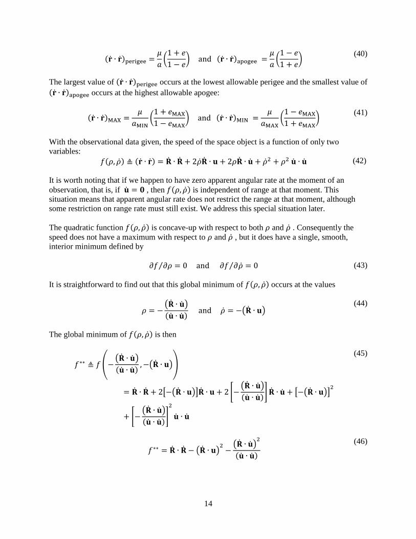
It is straightforward to verify the identities 𝐮 ∙ 𝐮 ≡ 1 and 𝐮 ∙ �̇� ≡ 0 . We note also that the expression (�̇� ∙ �̇�) , which occurs frequently in the following development, has a convenient and intuitive interpretation: (�̇� ∙ �̇�) = sin2 𝛿 (cos2 𝛼 + sin2 𝛼) �̇�2 + cos2 𝛿 (sin2 𝛼 + cos2 𝛼) �̇�2 + cos2 𝛿 �̇�2 (37) (�̇� ∙ �̇�) = �̇�2 + cos2 𝛿 �̇�2 (38) Hence (�̇� ∙ �̇�) is just the square of the total apparent angular rate. A similar expression would hold if the observation had been made in terms of azimuth and elevation angles and the rates of these. For short target detection streaks on the camera focal plane, the quantity (∆𝛿)2 + cos2 𝛿 (∆𝛼)2 is just the square of the length of the streak on the plane of the sky and the corresponding time difference ∆𝑡 would be the time elapsed between the endpoints of the streak. Now the magnitude of the velocity of the space object is obtained from ‖�̇�‖2 = �̇� ∙ �̇� = �̇� ∙ �̇� + 2�̇��̇� ∙ 𝐮 + 2𝜌�̇� ∙ �̇� + �̇�2 + 𝜌2�̇� ∙ �̇� (39) Here we have used the identities 𝐮 ∙ 𝐮 ≡ 1 and 𝐮 ∙ �̇� ≡ 0 , the latter of which has the effect of removing terms that contain both range and range rate. The bounds we seek are based on the fact that �̇� ∙ �̇� has a maximum value at perigee and a minimum value at apogee. In particular, the energy equation evaluated at perigee and apogee gives us

14

(�̇� ∙ �̇�)perigee =𝜇𝑎�

1 + 𝑒1 − 𝑒

� and (�̇� ∙ �̇�)apogee =𝜇𝑎�

1 − 𝑒1 + 𝑒

� (40)

The largest value of (�̇� ∙ �̇�)perigee occurs at the lowest allowable perigee and the smallest value of (�̇� ∙ �̇�)apogee occurs at the highest allowable apogee: (�̇� ∙ �̇�)MAX =

𝜇𝑎MIN

�1 + 𝑒MAX1 − 𝑒MAX

� and (�̇� ∙ �̇�)MIN =𝜇

𝑎MAX�

1 − 𝑒MAX1 + 𝑒MAX

� (41)

With the observational data given, the speed of the space object is a function of only two variables: 𝑓(𝜌, �̇�) ≜ (�̇� ∙ �̇�) = �̇� ∙ �̇� + 2�̇��̇� ∙ 𝐮 + 2𝜌�̇� ∙ �̇� + �̇�2 + 𝜌2 �̇� ∙ �̇� (42) It is worth noting that if we happen to have zero apparent angular rate at the moment of an observation, that is, if �̇� = 𝟎 , then 𝑓(𝜌, �̇�) is independent of range at that moment. This situation means that apparent angular rate does not restrict the range at that moment, although some restriction on range rate must still exist. We address this special situation later. The quadratic function 𝑓(𝜌, �̇�) is concave-up with respect to both 𝜌 and �̇� . Consequently the speed does not have a maximum with respect to 𝜌 and �̇� , but it does have a single, smooth, interior minimum defined by 𝜕𝑓 𝜕𝜌⁄ = 0 and 𝜕𝑓 𝜕�̇�⁄ = 0 (43) It is straightforward to find out that this global minimum of 𝑓(𝜌, �̇�) occurs at the values

𝜌 = −��̇� ∙ �̇��(�̇� ∙ �̇�) and �̇� = −��̇� ∙ 𝐮�

(44)

The global minimum of 𝑓(𝜌, �̇�) is then

𝑓∗∗ ≜ 𝑓 �−��̇� ∙ �̇��(�̇� ∙ �̇�) ,−��̇� ∙ 𝐮��

= �̇� ∙ �̇� + 2�−��̇� ∙ 𝐮��̇� ∙ 𝐮 + 2 �−��̇� ∙ �̇��(�̇� ∙ �̇�)� �̇� ∙ �̇� + �−��̇� ∙ 𝐮��

2

+ �−��̇� ∙ �̇��(�̇� ∙ �̇�)�

2

�̇� ∙ �̇�

(45)

𝑓∗∗ = �̇� ∙ �̇� − ��̇� ∙ 𝐮�2−��̇� ∙ �̇��

2

(�̇� ∙ �̇�) (46)

15

𝑓∗∗ = �̇� ∙ ��̇� − ��̇� ∙ 𝐮�𝐮 −

��̇� ∙ �̇��̇�(�̇� ∙ �̇�) �

(47)

Resolve the station velocity in the following orthonormal basis:

�̇� = ��̇� ∙ 𝐮�𝐮 + ��̇� ∙�̇�‖�̇�‖

��̇�‖�̇�‖

+ ��̇� ∙ �𝐮 ×�̇�‖�̇�‖

�� 𝐮 ×�̇�‖�̇�‖

� (48)

We see that the square bracket in equation (47) is just the third component of the station velocity in this orthonormal basis, so that

𝑓∗∗ = �̇� ∙ ��̇� ∙ �𝐮 ×�̇�‖�̇�‖

�� 𝐮 ×�̇�‖�̇�‖

�� = ��̇� ∙ �𝐮 ×�̇�‖�̇�‖

��2

(49)

In any case, 𝑓∗∗ is the square of the smallest possible orbital speed that is consistent with given values of �̇� , 𝐮 and �̇� . The value 𝑓∗∗ may not be physically realizable if the minimizing range value in (44) happens to be negative, although it is always a global lower bound on the possible values of orbital speed-squared. In case ��̇� ∙ �̇�� < 0 , the minimizing value of range is positive so the value 𝑓∗∗ is physically realizable. On the other hand, if ��̇� ∙ �̇�� > 0 then the minimizing value of range is negative. In the latter case, we can find an associated constrained minimum that is physically realizable. Because the value of 𝑓(𝜌, �̇�) is monotonic in 𝜌 as we move away from the global minimum value 𝑓∗∗ in any direction, we consider the value of the speed-squared at the first non-negative value of range that we come to, namely, 𝜌 = 0 : 𝑓∗ ≜ 𝑓 �0,−��̇� ∙ 𝐮�� (50)

Necessarily we have 𝑓(𝜌, �̇�) ≥ 𝑓∗ ≥ 𝑓∗∗, because we require a priori that range be non-negative. However, if ��̇� ∙ �̇�� > 0 , then 𝑓∗ , rather than 𝑓∗∗ , is the square of the smallest possible orbital speed that is consistent with given values of �̇� , 𝐮 and �̇� . Evaluating the speed-squared (42) as in the definition (50), we get 𝑓∗ = �̇� ∙ �̇� + 2�−��̇� ∙ 𝐮��̇� ∙ 𝐮 + 2[0]�̇� ∙ �̇� + �−��̇� ∙ 𝐮��

2+ [0]2 �̇� ∙ �̇� (51)

𝑓∗ = �̇� ∙ �̇� − ��̇� ∙ 𝐮�

2 (52)

𝑓∗ = �̇� ∙ ��̇� − ��̇� ∙ 𝐮�𝐮� (53) The square bracket is the projection of the station velocity on the plane normal to the line of sight. In terms of the orthonormal basis in equation (48) above, we could also write

16

𝑓∗ = �̇� ∙ ��̇� ∙

�̇�‖�̇�‖

��̇�‖�̇�‖

+ ��̇� ∙ �𝐮 ×�̇�‖�̇�‖

�� 𝐮 ×�̇�‖�̇�‖

�� (54)

𝑓∗ = ��̇� ∙�̇�‖�̇�‖

�2

+ ��̇� ∙ �𝐮 ×�̇�‖�̇�‖

��2

= 𝑓∗∗ + ��̇� ∙�̇�‖�̇�‖

�2

(55)

The distinction between the global minimum 𝑓∗∗ and the physically constrained minimum 𝑓∗ will become important later when we consider bounds on range rate. Until then we are seeking bounds only on the range. Consider the perigee case, and require the orbital speed-squared to be at most equal to the specified maximum orbital speed-squared. Using equation (42), we can write

𝑓(𝜌, �̇�) = �̇� ∙ �̇� + 2�̇��̇� ∙ 𝐮 + 2𝜌�̇� ∙ �̇� + �̇�2 + 𝜌2 �̇� ∙ �̇� ≤𝜇

𝑎MIN�

1 + 𝑒MAX1 − 𝑒MAX

� (56)

We note that this inequality still holds if we evaluate 𝑓(𝜌, �̇�) at its minimum with respect to �̇�, a minimum which is always physically realizable as long as the range is non-negative a priori:

𝑓 �𝜌 ,−��̇� ∙ 𝐮�� ≤𝜇

𝑎MIN�


� (57)

This derived inequality is independent of range rate and is a condition that has to be satisfied by the range when we have both angle and angle-rate values available. The substitution for �̇� lowers the value of 𝑓(𝜌, �̇�) compared to the value we would have had with the true (non-minimizing) value of �̇� , in effect relaxing the condition on range. However, with only angle and angle-rate values available, we apparently cannot do any better with the expression (56) if we want an explicit bound on range a priori. Rewriting (56) with the substitution (44) for �̇� , we get

�̇� ∙ �̇� − ��̇� ∙ 𝐮�2

+ 2𝜌�̇� ∙ �̇� + 𝜌2 �̇� ∙ �̇� ≤𝜇

𝑎MIN�


� (58)

(�̇� ∙ �̇�)𝜌2 + 2��̇� ∙ �̇��𝜌 − �

𝜇𝑎MIN


� − �̇� ∙ ��̇� − ��̇� ∙ 𝐮�𝐮�� ≤ 0 (59)

According to equation (53) above, we could re-write this as (�̇� ∙ �̇�)𝜌2 + 2��̇� ∙ �̇��𝜌 − �

𝜇𝑎MIN


� − 𝑓∗� ≤ 0 (60)

The roots of this quadratic are

17

𝜌 =

1(�̇� ∙ �̇�)�−��̇� ∙ �̇�� ± ��̇� ∙ �̇��

2+ (�̇� ∙ �̇�) �

𝜇𝑎MIN


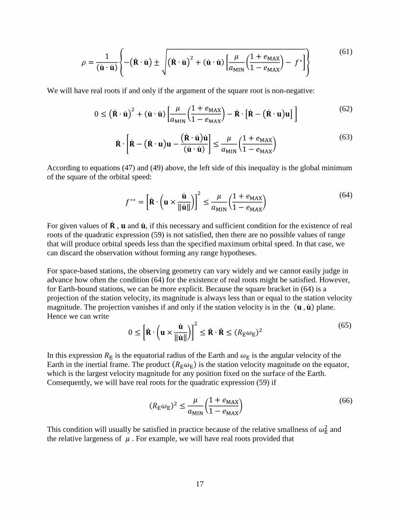
� − 𝑓∗�� (61)

We will have real roots if and only if the argument of the square root is non-negative:

0 ≤ ��̇� ∙ �̇��2

+ (�̇� ∙ �̇�) �𝜇

𝑎MIN�


� − �̇� ∙ ��̇� − ��̇� ∙ 𝐮�𝐮� � (62)

�̇� ∙ ��̇� − ��̇� ∙ 𝐮�𝐮 −��̇� ∙ �̇��̇�(�̇� ∙ �̇�) � ≤

𝜇𝑎MIN


� (63)

According to equations (47) and (49) above, the left side of this inequality is the global minimum of the square of the orbital speed:

𝑓∗∗ = ��̇� ∙ �𝐮 ×�̇�‖�̇�‖

��2

≤𝜇

𝑎MIN�


� (64)

For given values of �̇� , 𝐮 and �̇�, if this necessary and sufficient condition for the existence of real roots of the quadratic expression (59) is not satisfied, then there are no possible values of range that will produce orbital speeds less than the specified maximum orbital speed. In that case, we can discard the observation without forming any range hypotheses. For space-based stations, the observing geometry can vary widely and we cannot easily judge in advance how often the condition (64) for the existence of real roots might be satisfied. However, for Earth-bound stations, we can be more explicit. Because the square bracket in (64) is a projection of the station velocity, its magnitude is always less than or equal to the station velocity magnitude. The projection vanishes if and only if the station velocity is in the (𝐮 , �̇�) plane. Hence we can write

0 ≤ ��̇� ∙ �𝐮 ×�̇�‖�̇�‖

��2

≤ �̇� ∙ �̇� ≤ (𝑅E𝜔E)2 (65)

In this expression 𝑅E is the equatorial radius of the Earth and 𝜔E is the angular velocity of the Earth in the inertial frame. The product (𝑅E𝜔E) is the station velocity magnitude on the equator, which is the largest velocity magnitude for any position fixed on the surface of the Earth. Consequently, we will have real roots for the quadratic expression (59) if (𝑅E𝜔E)2 ≤

𝜇𝑎MIN


� (66)

This condition will usually be satisfied in practice because of the relative smallness of 𝜔E

2 and the relative largeness of 𝜇 . For example, we will have real roots provided that

18

𝑎MIN ≤𝜇

(𝑅E𝜔E)2 �1 + 𝑒MAX1 − 𝑒MAX

� ≅1 CDU3 CTU2⁄

�(1 CDU) � 2𝜋 rad86,164 sec� �

806.81 sec1 CTU ��

2 �1 + 𝑒MAX1 − 𝑒MAX

�

≅ �1 + 𝑒MAX1 − 𝑒MAX

� × 289 CDU (Earth radii)

(67)

Now, assuming that real roots for the quadratic (60) do exist, we consider whether the quadratic has any positive real roots. Descartes’ rule of signs tells us that (60) will have one real positive root, and therefore also one negative real root, if the third coefficient is negative, regardless of the sign of the second coefficient. The third coefficient is negative provided that

𝑓∗ = �̇� ∙ ��̇� − ��̇� ∙ 𝐮�𝐮� <𝜇

𝑎MIN�


� (68)

This condition must hold for observations from both Earth-bound and space-based stations. The square bracket is the projection of the station velocity on the plane normal to the line of sight, so its magnitude must be less than or equal to the station velocity magnitude. Hence, for Earth-bound stations, we can reason as before that we are guaranteed a single positive real root provided that

0 ≤ �̇� ∙ ��̇� − ��̇� ∙ 𝐮�𝐮� ≤ �̇� ∙ �̇� ≤ (𝑅E𝜔E)2 <𝜇

𝑎MIN�


� (69)

This expression is essentially the same as (66) above. We conclude that, in most practical cases, we can expect one real positive root and therefore also one negative root. Because the quadratic is concave-up, the inequality (60) will be satisfied between the roots. Excluding negative values of the range a priori, we can say in practice that the inequality is satisfied between 𝜌 = 0 and the one positive root:

0 ≤ 𝜌 ≤1

(�̇� ∙ �̇�)�−��̇� ∙ �̇�� + ��̇� ∙ �̇��2

+ (�̇� ∙ �̇�) �𝜇

𝑎MIN�


� − 𝑓∗�� (70)

If the third coefficient in (60) is positive, then we will have either zero or two positive real roots, depending on whether the second coefficient is positive or negative. If, in this case, the second coefficient is negative, ��̇� ∙ �̇�� < 0 , then we will have two positive real roots. The quadratic is concave-up, so the inequality is satisfied between the two positive roots:

𝜌 ≥1

(�̇� ∙ �̇�)�−��̇� ∙ �̇�� − ��̇� ∙ �̇��2

+ (�̇� ∙ �̇�) �𝜇

𝑎MIN�


� − 𝑓∗�� (71)

𝜌 ≤1

(�̇� ∙ �̇�)�−��̇� ∙ �̇�� + ��̇� ∙ �̇��2

+ (�̇� ∙ �̇�) �𝜇

𝑎MIN�


� − 𝑓∗�� (72)

19

If both the second and third coefficients in (60) are positive, we have no positive real roots, only two negative roots, and the inequality is satisfied between them. In this case, we can discard the observation and form no range hypotheses for it because we exclude negative values of the range a priori. Hence, whenever we have one or two positive real roots, we will have an upper bound on the possible values of the range 𝜌 :

𝜌 ≤1

(�̇� ∙ �̇�)�−��̇� ∙ �̇�� + ��̇� ∙ �̇��2

+ (�̇� ∙ �̇�) �𝜇

𝑎MIN�


� − 𝑓∗�� (73)

This upper bound, based on maximum orbital speed at perigee, is compatible with the observed angular rate values and also compatible with the specified limits on semimajor axis and eccentricity. There might also be a positive lower bound as in the inequality (71) described above. Now consider the apogee case. We require that the orbital speed be no smaller than the smallest allowable orbital speed: 𝜇

𝑎MAX�


� ≤ 𝑓(𝜌, �̇�) (74)

The problem here is to assign an upper bound with respect to �̇� to the function 𝑓(𝜌, �̇�) when no interior maximum with respect to range rate exists. If we can assign such a bound, we are left with a quadratic expression involving only range. Necessarily, any a priori assignment, depending only on the observation, must be somewhat arbitrary. If we assign a too-optimistic (low) upper bound, then the condition to be satisfied by 𝜌 will be too constrained and we may miss some values of range that would otherwise lead to candidate orbits within the given element-set partition. If we assign a too-conservative (high) upper bound, then the condition to be satisfied by 𝜌 will be too relaxed and we will have to check possibly many range values that lead to orbits outside the given element-set partition. In practice, missing possible candidate orbits is a more serious error than having to check too many cases, because the overall computation is parallelizable. Hence, we want to be somewhat conservative in how we assign the upper bound, but we do not want to be overly so. Recall from equation (42) and following expressions that the global minimum of 𝑓(𝜌, �̇�) with respect to �̇� occurs at the special value �̇� = −��̇� ∙ 𝐮� . Moreover, the function 𝑓(𝜌, �̇�) is monotonic-increasing with respect to �̇� as we move away from the global minimum. It is also symmetric with respect to the minimum along the �̇� axis. Therefore we will seek to move to a value of �̇� that is as far from this global minimum as possible while still being consistent with the given element-set partition and the given observational data. The largest allowable magnitude of �̇� would occur when the station velocity is aligned with the orbital velocity and the latter is at its maximum magnitude, namely at the lowest allowable perigee:

20

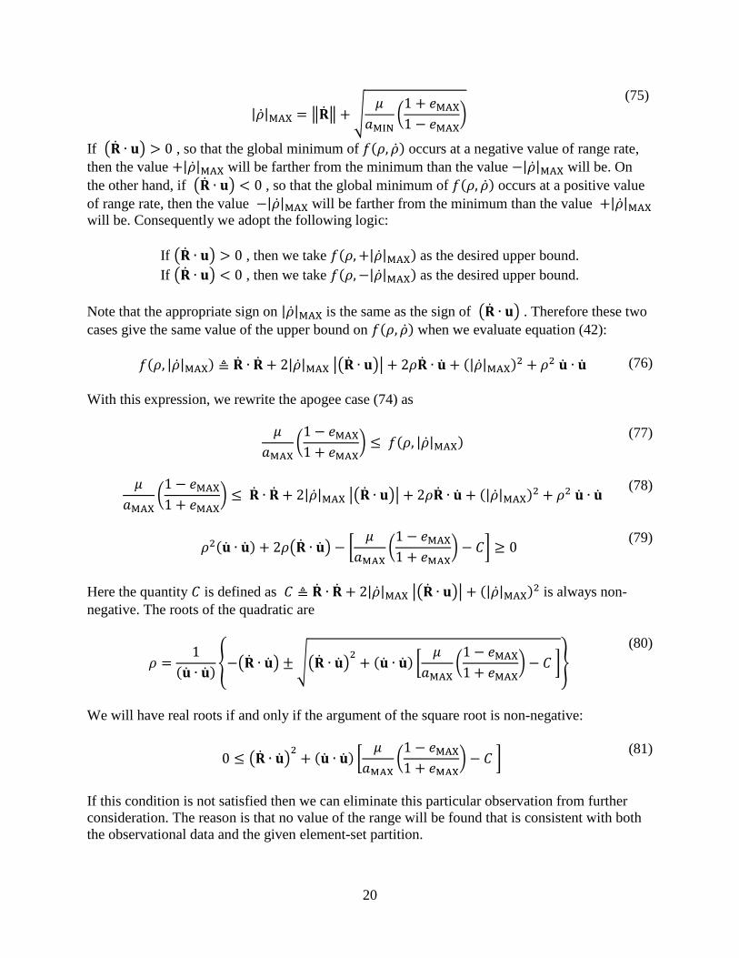
|�̇�|MAX = ��̇�� + �

𝜇𝑎MIN


� (75)

If ��̇� ∙ 𝐮� > 0 , so that the global minimum of 𝑓(𝜌, �̇�) occurs at a negative value of range rate, then the value +|�̇�|MAX will be farther from the minimum than the value −|�̇�|MAX will be. On the other hand, if ��̇� ∙ 𝐮� < 0 , so that the global minimum of 𝑓(𝜌, �̇�) occurs at a positive value of range rate, then the value −|�̇�|MAX will be farther from the minimum than the value +|�̇�|MAX will be. Consequently we adopt the following logic:

If ��̇� ∙ 𝐮� > 0 , then we take 𝑓(𝜌, +|�̇�|MAX) as the desired upper bound. If ��̇� ∙ 𝐮� < 0 , then we take 𝑓(𝜌,−|�̇�|MAX) as the desired upper bound.

Note that the appropriate sign on |�̇�|MAX is the same as the sign of ��̇� ∙ 𝐮� . Therefore these two cases give the same value of the upper bound on 𝑓(𝜌, �̇�) when we evaluate equation (42): 𝑓(𝜌, |�̇�|MAX) ≜ �̇� ∙ �̇� + 2|�̇�|MAX ��̇� ∙ 𝐮�� + 2𝜌�̇� ∙ �̇� + (|�̇�|MAX)2 + 𝜌2 �̇� ∙ �̇� (76) With this expression, we rewrite the apogee case (74) as 𝜇

𝑎MAX�


� ≤ 𝑓(𝜌, |�̇�|MAX) (77)

𝜇

𝑎MAX�


� ≤ �̇� ∙ �̇� + 2|�̇�|MAX ��̇� ∙ 𝐮�� + 2𝜌�̇� ∙ �̇� + (|�̇�|MAX)2 + 𝜌2 �̇� ∙ �̇� (78)

𝜌2(�̇� ∙ �̇�) + 2𝜌��̇� ∙ �̇�� − �𝜇

𝑎MAX�


� − 𝐶� ≥ 0 (79)

Here the quantity 𝐶 is defined as 𝐶 ≜ �̇� ∙ �̇� + 2|�̇�|MAX ��̇� ∙ 𝐮�� + (|�̇�|MAX)2 is always non-negative. The roots of the quadratic are

𝜌 =1

(�̇� ∙ �̇�)�−��̇� ∙ �̇�� ± ��̇� ∙ �̇��2

+ (�̇� ∙ �̇�) �𝜇

𝑎MAX�


� − 𝐶 �� (80)

We will have real roots if and only if the argument of the square root is non-negative:

0 ≤ ��̇� ∙ �̇��2

+ (�̇� ∙ �̇�) �𝜇

𝑎MAX�


� − 𝐶 � (81)

If this condition is not satisfied then we can eliminate this particular observation from further consideration. The reason is that no value of the range will be found that is consistent with both the observational data and the given element-set partition.

21

Investigating this condition for the existence of real roots more closely, we substitute for |�̇�|MAX in the definition of 𝐶 :

𝐶 = �̇� ∙ �̇� + 2 ��̇�� + �𝜇

𝑎MIN�


�� ̇� ∙ 𝐮�� + ��̇�� + �𝜇

𝑎MIN�


��

2

(82)

𝐶 = 2��̇��2

+ 2��̇�� ̇�𝑖 ∙ 𝐮𝑖�� + 2��̇� ∙ 𝐮��𝜇

𝑎MIN�


�

+ 2��̇��𝜇

𝑎MIN�


� +𝜇

𝑎MIN�


�

(83)

Consequently, the following inequality always holds, even for zero station velocity:

𝐶 =𝜇

𝑎MIN�


� + non-negative terms > 𝜇

𝑎MAX�


� (84)

This means that the third coefficient (the constant term) in the quadratic form (79) is always positive, given this choice of 𝐶. Assuming that real roots exist, the quadratic will have either zero or two positive real roots, depending on the sign of the second coefficient. If ��̇� ∙ �̇�� > 0 then we have no positive roots, only two negative roots. The quadratic is concave-up so the inequality is satisfied to the left of the left-most root and to the right of the right-most root. However, this condition reduces merely to 𝜌 ≥ 0 because we require a priori that the range be non-negative. If the second coefficient is negative, ��̇� ∙ �̇�� < 0 , then the quadratic has two positive real roots. Again, because the quadratic is concave-up, the inequality is satisfied between 𝜌 = 0 and the left-most root and to the right of the right-most root:

0 ≤ 𝜌 ≤1

(�̇� ∙ �̇�)�−��̇� ∙ �̇�� − ��̇� ∙ �̇��2

+ (�̇� ∙ �̇�) �𝜇

𝑎MAX�


� − 𝐶 �� (85)

𝜌 ≥1

(�̇� ∙ �̇�)�−��̇� ∙ �̇�� + ��̇� ∙ �̇��2

+ (�̇� ∙ �̇�) �𝜇

𝑎MAX�


� − 𝐶 �� (86)

22

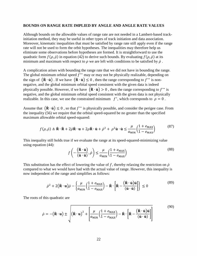
BOUNDS ON RANGE RATE IMPLIED BY ANGLE AND ANGLE RATE VALUES Although bounds on the allowable values of range rate are not needed in a Lambert-based track-initiation method, they may be useful in other types of track initiation and data association. Moreover, kinematic inequalities that must be satisfied by range rate still apply even if the range rate will not be used to form the orbit hypotheses. The inequalities may therefore help us eliminate some observations before hypotheses are formed. It is straightforward to use the quadratic form 𝑓(𝜌, �̇�) in equation (42) to derive such bounds. By evaluating 𝑓(𝜌, �̇�) at its minimum and maximum with respect to 𝜌 we are left with conditions to be satisfied by �̇� . A complication arises with bounding the range rate that we did not have in bounding the range. The global minimum orbital speed 𝑓∗∗ may or may not be physically realizable, depending on the sign of ��̇� ∙ �̇�� . If we have ��̇� ∙ �̇�� ≤ 0 , then the range corresponding to 𝑓∗∗ is non-negative, and the global minimum orbital speed consistent with the given data is indeed physically possible. However, if we have ��̇� ∙ �̇�� > 0 , then the range corresponding to 𝑓∗∗ is negative, and the global minimum orbital speed consistent with the given data is not physically realizable. In this case, we use the constrained minimum 𝑓∗, which corresponds to 𝜌 = 0 . Assume that ��̇� ∙ �̇�� ≤ 0 , so that 𝑓∗∗ is physically possible, and consider the perigee case. From the inequality (56) we require that the orbital speed-squared be no greater than the specified maximum allowable orbital speed-squared:

𝑓(𝜌, �̇�) ≜ �̇� ∙ �̇� + 2�̇��̇� ∙ 𝐮 + 2𝜌�̇� ∙ �̇� + �̇�2 + 𝜌2�̇� ∙ �̇� ≤𝜇

𝑎MIN�


� (87)

This inequality still holds true if we evaluate the range at its speed-squared-minimizing value using equation (44):

𝑓 �−��̇� ∙ �̇��(�̇� ∙ �̇�) , �̇�� ≤

𝜇𝑎MIN


� (88)

This substitution has the effect of lowering the value of 𝑓, thereby relaxing the restriction on �̇� compared to what we would have had with the actual value of range. However, this inequality is now independent of the range and simplifies as follows:

�̇�2 + 2��̇� ∙ 𝐮��̇� − �𝜇

𝑎MIN�


� − �̇� ∙ ��̇� −��̇� ∙ �̇��̇�(�̇� ∙ �̇�) �� ≤ 0

(89)


�̇� = −��̇� ∙ 𝐮� ± ��̇� ∙ 𝐮�2

+ �𝜇

𝑎MIN�


� − �̇� ∙ ��̇� −��̇� ∙ �̇��̇�(�̇� ∙ �̇�) ��

(90)

23

In order to guarantee that the roots are real, it is necessary and sufficient that the argument of the square root be non-negative:

�̇� ∙ ��̇� − ��̇� ∙ 𝐮�𝐮 −��̇� ∙ �̇��̇�(�̇� ∙ �̇�) � ≤

𝜇𝑎MIN


� (91)

According to equations (47) – (49) above, the left side of this inequality is simply the global minimum of the square of the orbital speed:

𝑓∗∗ = ��̇� ∙ �𝐮 ×�̇�‖�̇�‖

��2

≤𝜇

𝑎MIN�


� (92)

For a given observation, if this necessary and sufficient condition for the existence of real roots of the quadratic expression (89) is not satisfied, then there are no possible values of range rate that will produce orbital speeds less than the specified maximum orbital speed. In that case, we can discard the given data without forming any range or range rate hypotheses. For space-based stations, the observing geometry can vary widely and we cannot easily judge in advance how often the condition (92) for the existence of real roots might be satisfied. However, for Earth-bound stations, we can be more explicit. Because the square bracket in (92) is a projection of the station velocity, its magnitude is always less than or equal to the station velocity magnitude. The projection vanishes only if the station velocity is in the (𝐮 , �̇�) plane. Hence we can write

0 ≤ ��̇� ∙ �𝐮 ×�̇�‖�̇�‖

��2

≤ �̇� ∙ �̇� ≤ (𝑅E𝜔E)2 (93)

Consequently, we will have real roots for the quadratic expression (89) if (𝑅E𝜔E)2 ≤

𝜇𝑎MIN


� (94)

This condition is the same as (66) above, so we can usually expect to have real roots in the case of Earth-bound observations. Now, assuming that real roots for the quadratic (89) do exist, we consider whether the quadratic has any positive real roots. Descartes’ rule of signs tells us that (89) will have one positive real root, and therefore also one negative real root, if the third coefficient is negative, regardless of the sign of the second coefficient. The third coefficient is negative provided that

�̇� ∙ ��̇� −��̇� ∙ �̇��̇�(�̇� ∙ �̇�) � <

𝜇𝑎MIN


� (95)

This condition must hold for observations from both Earth-bound and space-based stations, if we are to have one positive real root of the quadratic (89). The square bracket is a projection of the station velocity, so its magnitude must be less than or equal to the station velocity magnitude.

24

Hence, for Earth-bound stations, we can reason as before that we are guaranteed a single positive real root if

0 ≤ �̇� ∙ ��̇� −��̇� ∙ �̇��̇�(�̇� ∙ �̇�) � ≤ �̇� ∙ �̇� ≤ (𝑅E𝜔E)2 <

𝜇𝑎MIN


� (96)

This expression is essentially the same as (94) and (66) above. We conclude that, in most practical cases with Earth-bound stations, we can expect one real positive root and therefore necessarily also one negative root. Because the quadratic is concave-up, the inequality (89) will be satisfied between the roots:

�̇� ≥ −��̇� ∙ 𝐮� − ��̇� ∙ 𝐮�2

+ �𝜇

𝑎MIN�


� − �̇� ∙ ��̇� −��̇� ∙ �̇��̇�(�̇� ∙ �̇�) ��

(97)

�̇� ≤ −��̇� ∙ 𝐮� + ��̇� ∙ 𝐮�2

+ �𝜇

𝑎MIN�


� − �̇� ∙ ��̇� −��̇� ∙ �̇��̇�(�̇� ∙ �̇�) ��

(98)

These bounds apply in the perigee case whenever ��̇� ∙ �̇�� ≤ 0 . Now consider the apogee case when ��̇� ∙ �̇�� ≤ 0 . From the inequality (42) we have 𝜇

𝑎MAX�


� ≤ 𝑓(𝜌, �̇�) (99)

Analogously with the case of range, inequality (74), we seek to assign a somewhat conservative (high) upper bound on the value of 𝑓(𝜌, �̇�) with respect to 𝜌 . In practice, we do not want the upper bound to be too conservative, because that would relax the condition on �̇� too much and lead us to have to check too many values of range rate. Of course, this is a less serious difficulty than having a too-optimistic (low) upper bound on the value of 𝑓(𝜌, �̇�) . The latter would make the resulting condition on �̇� too constraining and lead us to miss values of range rate that would have produced candidate orbits within the given element-set partition. Recall from (44) that the value of range at the minimum of 𝑓(𝜌, �̇�)with respect to range is 𝜌 = −��̇� ∙ �̇�� (�̇� ∙ �̇�)⁄ , regardless of the sign of this quantity. Note also that 𝑓(𝜌, �̇�) is monotonic-increasing with respect to 𝜌 as we move away from this minimum. Also, for every value of range rate, the function 𝑓(𝜌, �̇�) is symmetric with respect to the minimum along the 𝜌 coordinate direction. Therefore, we will seek to move to a value of 𝜌 that is as far from the minimum as possible while still being consistent with the given element-set partition and the given observation. Of course, we will require that the range be non-negative a priori. In fact, the largest allowable value of 𝜌 has already been derived. From equation (14), we have:

𝜌MAX = −(𝐑 ∙ 𝐮) + �(𝐑 ∙ 𝐮)2 + [𝑎MAX2 (1 + 𝑒MAX)2 − 𝐑 ∙ 𝐑] (100)

25

The largest possible value of this function would occur when 𝐑 is aligned with −𝐮 , leaving 𝜌MAX = ‖𝐑‖ + 𝑎MAX(1 + 𝑒MAX) . In this case, the station position would be aligned with the perigee of the orbit while the satellite is at the highest allowable apogee. In practice, this extreme value of maximum range cannot occur because the size of the Earth prevents this viewing geometry. The more general equation (100) accounts for the actual viewing geometry. We require that this maximum range (100) be real-valued, just as we did for equation (14). Hence, the condition (13) applies here also: 𝑎MAX2 (1 + 𝑒MAX)2 ≥ 𝐑 ∙ [𝐑 − (𝐑 ∙ 𝐮)𝐮] . In particular, if this latter condition does not hold, then no possible value of the range will lead to orbits within the specified element partition. We can discard the observation without forming any hypotheses for it. If the range for the minimum of 𝑓(𝜌, �̇�) with respect to range were to take the value 1

2𝜌MAX ,

halfway between 𝜌 = 0 and 𝜌 = 𝜌MAX , then we would have 𝑓(0, �̇�) = 𝑓(𝜌MAX, �̇�) because of symmetry of the function. If the global minimum were to the left of 1

2𝜌MAX then we would have

𝑓(0, �̇�) < 𝑓(𝜌MAX, �̇�) , and if the minimum were to the right of 12𝜌MAX then we would have

𝑓(0, �̇�) > 𝑓(𝜌MAX, �̇�) . Moreover, if ��̇� ∙ �̇�� > 0 , so that the minimum of 𝑓(𝜌, �̇�) occurs at a negative value of the range, then the value 𝜌 = 𝜌MAX is always farther from the minimum than is the value 𝜌 = 0 . In that case we always have 𝑓(0, �̇�) ≤ 𝑓(𝜌MAX, �̇�) . On the other hand, if ��̇� ∙ �̇�� < 0 , so that the minimum occurs at a positive value of the range, then either 𝜌 = 0 or 𝜌 = 𝜌MAX could be farther from the minimum, depending on the exact value of ��̇� ∙ �̇�� . The following logic includes all cases for assigning an upper bound with respect to range for the function 𝑓(𝜌, �̇�) :

If −��̇� ∙ �̇�� (�̇� ∙ �̇�)⁄ ≤ 𝜌MAX 2⁄ , then the upper bound on 𝑓(𝜌, �̇�) is 𝑓(𝜌MAX, �̇�) . If −��̇� ∙ �̇�� (�̇� ∙ �̇�)⁄ > 𝜌MAX 2⁄ , then the upper bound on 𝑓(𝜌, �̇�) is 𝑓(0, �̇�) .

Therefore, for the apogee case, inequality (99), we need to consider these two sub-cases. First consider the sub-case 𝜇

𝑎MAX�


� ≤ 𝑓(𝜌MAX, �̇�) (101)

𝜇

𝑎MAX�


� ≤ �̇� ∙ �̇� + 2�̇��̇� ∙ 𝐮 + 2𝜌MAX�̇� ∙ �̇� + �̇�2 + 𝜌MAX2 �̇� ∙ �̇� (102)

�̇�2 + 2�̇��̇� ∙ 𝐮 − �𝜇

𝑎MAX�


� − 𝐷� ≥ 0 (103)

Here the quantity 𝐷 ≜ �̇� ∙ �̇� + 2𝜌MAX�̇� ∙ �̇� + 𝜌MAX2 �̇� ∙ �̇� = ��̇� + 𝜌MAX�̇�� ∙ ��̇� + 𝜌MAX�̇�� is always non-negative. The roots of the quadratic are

26

�̇� = −��̇� ∙ 𝐮� ± ��̇� ∙ 𝐮�

2+ �

𝜇𝑎MAX

�1 − 𝑒MAX1 + 𝑒MAX

� − 𝐷� (104)

and real roots will exist if and only if the argument of the square root is non-negative:

��̇� ∙ 𝐮�2

+ �𝜇

𝑎MAX�


� − 𝐷� ≥ 0 (105)

If no real roots exist, then no value of the range rate can be found that results in orbital velocities greater than the minimum allowable, for the given element-set partition and the given observation. As we noted earlier, this means that the particular observation in question can be excluded from further consideration in forming orbit hypotheses, even if hypotheses are being formed without explicitly using range rate, as in the Lambert-based approach. If real roots exist, then the inequality is satisfied to the left of the left-most root and to the right of the right-most root, because the quadratic (103) is concave-up:

�̇� ≤ −��̇� ∙ 𝐮� − ��̇� ∙ 𝐮�2

+ �𝜇

𝑎MAX�


� − 𝐷� (106)

�̇� ≥ −��̇� ∙ 𝐮� + ��̇� ∙ 𝐮�2

+ �𝜇

𝑎MAX�


� − 𝐷� (107)

Now we consider the other sub-case for the apogee case. The inequality (99) becomes 𝜇

𝑎MAX�


� ≤ 𝑓(0, �̇�) (108)

Then, using (42) with 𝜌 = 0 , we get 𝜇

𝑎MAX�


� ≤ �̇� ∙ �̇� + 2�̇��̇� ∙ 𝐮 + �̇�2 (109)

Notice that setting 𝜌 = 0 causes all terms containing angle rate to vanish. Although angle rate does not constrain the range rate in this case, range rate must still satisfy this quadratic condition.

�̇�2 + 2�̇��̇� ∙ 𝐮 − �𝜇

𝑎MAX�


� − �̇� ∙ �̇�� ≥ 0 (110)

The roots of the quadratic are

�̇� = −��̇� ∙ 𝐮� ± ��̇� ∙ 𝐮�2

+ �𝜇

𝑎MAX�


� − �̇� ∙ �̇�� (111)

27

Real roots of the quadratic (110) exist if and only if the argument of the square root is non-negative: 𝜇

𝑎MAX�


� ≥ �̇� ∙ ��̇� − ��̇� ∙ 𝐮�𝐮� (112)

If this necessary and sufficient condition for the existence of real roots of the quadratic expression (110) is not satisfied, then there are no possible values of range rate that will produce orbital speeds greater than the specified minimum orbital speed. In that case, we can discard the given observation without forming any range or range rate hypotheses. For space-based stations, the observing geometry can vary widely and we cannot easily judge in advance how often the condition (112) for the existence of real roots might be satisfied. However, for Earth-bound stations, we can be more explicit. Because the square bracket in (112) is a projection of the station velocity, its magnitude is always less than or equal to the station velocity magnitude. The projection vanishes only if the station velocity is aligned with the line-of-sight unit vector 𝐮 . Hence we can write 0 ≤ �̇� ∙ ��̇� − ��̇� ∙ 𝐮�𝐮� ≤ �̇� ∙ �̇� ≤ (𝑅E𝜔E)2 (113) Consequently, we will have real roots for the quadratic expression (121) if (𝑅E𝜔E)2 ≤

𝜇𝑎MAX


� (114)

This condition is analogous to (66) and similar expressions given above for the perigee cases. Let us examine the conditions under which we can expect it to be satisfied. Following the reasoning in (66), we can write 𝑎MAX ≤

𝜇(𝑅E𝜔E)2 �


� ≅1 CDU3 CTU2⁄

�(1 CDU) � 2𝜋 rad86,164 sec� �

806.81 sec1 CTU ��

2 �1 − 𝑒MAX1 + 𝑒MAX

�

≅ �1 − 𝑒MAX1 + 𝑒MAX

� × 289 CDU (Earth radii)

(115)

For values of the maximum allowable eccentricity near unity, the maximum allowable semimajor axis that will guarantee the existence of real roots of (110) will be markedly restricted compared to the perigee case. For example, at 𝑒MAX = 0.9 , we have 𝑎MAX ≤ 15.2 CDU approximately. However, with eccentricity this large, we would also require 𝑎MIN ≥ 10.0 CDU in order to have a smallest allowable perigee greater than one Earth radius. We conclude that, at least in a useful number of low-maximum-eccentricity cases, we can expect real roots for (110) when we have observations from an Earth-bound station. Of course, we should always use the exact condition (112) to determine the existence of real roots for (110) rather than the very conservative approximate condition (114).

28

Now, assuming that real roots for the quadratic (110) do exist, we consider whether the quadratic has any positive real roots. Descartes’ rule of signs tells us that (110) will have one real positive root, and therefore also one negative real root, if the third coefficient is negative, regardless of the sign of the second coefficient. The third coefficient is negative provided that 𝜇

𝑎MAX�


� ≥ �̇� ∙ �̇� (116)

This condition must hold for observations for both Earth-bound and space-based stations, if we are to have one positive real root of the quadratic (110). For Earth-bound stations, we can reason as before that we are guaranteed a single positive real root if

0 ≤ �̇� ∙ �̇� ≤ (𝑅E𝜔E)2 <𝜇

𝑎MAX�


� (117)

This expression is essentially the same as (114) above. We conclude that, in many practical cases for Earth-bound stations, we can expect one real positive root and therefore necessarily also one negative root. Because the quadratic is concave-up, the inequality (110) will be satisfied to the left of the negative root and to the right of the positive root:

�̇� ≤ −��̇� ∙ 𝐮� − ��̇� ∙ 𝐮�2

+ �𝜇

𝑎MAX�


� − �̇� ∙ �̇�� (118)

�̇� ≥ −��̇� ∙ 𝐮� + ��̇� ∙ 𝐮�2

+ �𝜇

𝑎MAX�


� − �̇� ∙ �̇�� (119)

For space-based stations, the inequality (116) must be re-examined. The third coefficient of the quadratic expression in (110) will be negative only in case the smallest allowable apogee speed is greater than the station speed. For example, a station in circular orbit must be well above the highest allowable apogee for this to occur. However, if (116) is not satisfied, so that the third coefficient of (110) is positive, the number of positive real roots depends on the sign of the second coefficient. If �̇� ∙ 𝐮 > 0 , then (110) has no positive real roots, but two negative ones. The quadratic is concave up, so the inequality must be satisfied to the left of the more negative root and to the right of the less negative root. If �̇� ∙ 𝐮 < 0 , then (110) has two positive roots and the inequality is satisfied to the left of the smaller positive root and to the right of the larger positive root. In effect, the inequalities (118) and (119) include all possible cases of real roots for observations from both Earth-bound and space-based stations, in the apogee sub-case (108). Now consider the case ��̇� ∙ �̇�� > 0 , so that 𝑓∗∗ is not physically possible, and consider the perigee case. From (56), we have

𝑓(𝜌, �̇�) ≜ �̇� ∙ �̇� + 2�̇��̇� ∙ 𝐮 + 2𝜌�̇� ∙ �̇� + �̇�2 + 𝜌2 �̇� ∙ �̇� ≤𝜇

𝑎MIN�


� (120)

29

This inequality still holds true if we evaluate the range at its constrained speed-squared-minimizing value 𝜌 = 0 according to equation (50):

𝑓(0, �̇�) ≤𝜇

𝑎MIN�


� (121)

Here we note that this case is equivalent to the special case of �̇� = 𝟎 , zero apparent total angular rate, in the sense that the resulting inequalities for range rate are the same in both cases. When all vectors are resolved in an inertial frame, zero apparent angular rate would, of course, be an exceptional circumstance. Should it occur, however, the value of range is not restricted by angular rate at that moment, and any of the above analysis that involves division by total apparent angular rate does not apply. However, the range rate is still restricted in the manner about to be shown. The inequality (121) becomes

�̇�2 + 2�̇��̇� ∙ 𝐮 − �𝜇

𝑎MIN�


� − �̇� ∙ �̇�� ≤ 0 (122)


�̇� = −��̇� ∙ 𝐮� ± ��̇� ∙ 𝐮�2

+ �𝜇

𝑎MIN�


� − �̇� ∙ �̇�� (123)


𝑎MIN�


� ≥ �̇� ∙ ��̇� − ��̇� ∙ 𝐮�𝐮� (124)

For a given observation, if this necessary and sufficient condition for the existence of real roots of the quadratic expression (122) is not satisfied, then there are no possible values of range rate that will produce orbital speeds less than the specified maximum orbital speed. In that case, we can discard the observation without forming any range or range rate hypotheses for it. For space-based stations, the observing geometry can vary widely and we cannot easily judge in advance how often the condition (124) for the existence of real roots might be satisfied. However, for Earth-bound stations, we can be more explicit. Because the square bracket in (124) is a projection of the station velocity, its magnitude is always less than or equal to the station velocity magnitude. The projection vanishes only if the station velocity is aligned with 𝐮 . Hence we can write 0 ≤ �̇� ∙ ��̇� − ��̇� ∙ 𝐮�𝐮� ≤ �̇� ∙ �̇� ≤ (𝑅E𝜔E)2 (125) Consequently, we will have real roots for the quadratic expression (122) if

30

(𝑅E𝜔E)2 ≤𝜇

𝑎MIN�


� (126)

This condition is the same as (66) above, so we can usually expect to have real roots in the case of Earth-bound observations. Now, assuming that real roots for the quadratic (122) do exist, we consider whether the quadratic has any positive real roots. Descartes’ rule of signs tells us that (122) will have one real positive root, and therefore also one negative real root, if the third coefficient is negative, regardless of the sign of the second coefficient. The third coefficient is negative provided that 𝜇

𝑎MIN�


� ≥ �̇� ∙ �̇� (127)


0 ≤ �̇� ∙ �̇� ≤ (𝑅E𝜔E)2 <𝜇

𝑎MIN�


� (128)

This expression is essentially the same as (126) above. We conclude that, in most practical cases for Earth-bound stations, we can expect one real positive root and therefore necessarily also one negative root. Because the quadratic is concave-up, the inequality (122) will be satisfied between the roots:

�̇� ≥ −��̇� ∙ 𝐮� − ��̇� ∙ 𝐮�2

+ �𝜇

𝑎MIN�


� − �̇� ∙ �̇�� (129)

�̇� ≤ −��̇� ∙ 𝐮� + ��̇� ∙ 𝐮�2

+ �𝜇

𝑎MIN�


� − �̇� ∙ �̇�� (130)

For space-based stations, the inequality (127) must be re-examined. The third coefficient of the quadratic expression in (122) will be negative only in case the largest allowable perigee speed is greater than the station speed. For example, a station in circular orbit must be well above the lowest allowable perigee for this to occur. However, if (127) is not satisfied, so that the third coefficient of (122) is positive, the number of positive real roots depends on the sign of the second coefficient. If �̇� ∙ 𝐮 > 0 , then (122) has no positive real roots, but two negative ones. The quadratic is concave up, so the inequality must be satisfied between them. If �̇� ∙ 𝐮 < 0 , then (122) has two positive roots and the inequality is satisfied between them. In effect, the inequalities (129) and (130) include all possible cases of real roots in the perigee case whenever ��̇� ∙ �̇�� > 0 .

31

Now consider the apogee case. The expressions (41) and (42) together give us the requirement that the minimum orbital speed-squared be no less than the lowest allowable orbital speed-squared:

𝑓(𝜌, �̇�) ≜ �̇� ∙ �̇� + 2�̇��̇� ∙ 𝐮 + 2𝜌�̇� ∙ �̇� + �̇�2 + 𝜌2�̇� ∙ �̇� ≥𝜇

𝑎MAX�


� (131)

In the special cases �̇� = 𝟎 or 𝜌 = 0 , the inequality (131) becomes a function of range rate only:

�̇� ∙ �̇� + 2�̇��̇� ∙ 𝐮 + �̇�2 ≥𝜇

𝑎MAX�


� (132)

�̇�2 + 2�̇��̇� ∙ 𝐮 − �𝜇

𝑎MAX�


� − �̇� ∙ �̇�� ≥ 0 (133)

This expression is the same as (110). The roots of the quadratic are

�̇� = −��̇� ∙ 𝐮� ± ��̇� ∙ 𝐮�2

+ �𝜇

𝑎MAX�


� − �̇� ∙ �̇�� (134)


𝑎MAX�


� ≥ �̇� ∙ ��̇� − ��̇� ∙ 𝐮�𝐮� (135)

For a given observation, if this necessary and sufficient condition for the existence of real roots of the quadratic expression (133) is not satisfied, then there are no possible values of range rate that will produce orbital speeds less than the specified maximum orbital speed. In that case, we can discard the observation without forming any range or range rate hypotheses. For space-based stations, the observing geometry can vary widely and we cannot easily judge in advance how often the condition (135) for the existence of real roots might be satisfied. However, for Earth-bound stations, we can be more explicit. Because the square bracket in (135) is a projection of the station velocity, its magnitude is always less than or equal to the station velocity magnitude. The projection vanishes only if the station velocity is aligned with the line-of-sight unit vector 𝐮 . Hence we can write 0 ≤ �̇� ∙ ��̇� − ��̇� ∙ 𝐮�𝐮� ≤ �̇� ∙ �̇� ≤ (𝑅E𝜔E)2 (136) Consequently, we will have real roots for the quadratic expression (133) if (𝑅E𝜔E)2 ≤

𝜇𝑎MAX


� (137)

32

This condition is the same as (114) above, so we can usually expect to have real roots in the case of Earth-bound observations. Now, assuming that real roots for the quadratic (133) do exist, we consider whether the quadratic has any positive real roots. Descartes’ rule of signs tells us that (133) will have one real positive root, and therefore also one negative real root, if the third coefficient is negative, regardless of the sign of the second coefficient. The third coefficient is negative provided that 𝜇

𝑎MAX�


� ≥ �̇� ∙ �̇� (138)


0 ≤ �̇� ∙ �̇� ≤ (𝑅E𝜔E)2 <𝜇

𝑎MAX�


� (139)

This expression is essentially the same as (137) and (114) above. We conclude that, in most practical cases for Earth-bound stations, we can expect one real positive root and therefore necessarily also one negative root. Because the quadratic is concave-up, the inequality (133) will be satisfied to the left of the negative root and to the right of the positive root:

�̇� ≤ −��̇� ∙ 𝐮� − ��̇� ∙ 𝐮�2

+ �𝜇

𝑎MAX�


� − �̇� ∙ �̇�� (140)

�̇� ≥ −��̇� ∙ 𝐮� + ��̇� ∙ 𝐮�2

+ �𝜇

𝑎MAX�


� − �̇� ∙ �̇�� (141)

These expressions are the same as (118) and (119). For space-based stations, the inequality (138) must be re-examined. The third coefficient of the quadratic expression in (133) will be negative only in case the smallest allowable apogee speed is greater than the station speed. For example, a station in circular orbit must be well above the highest allowable apogee for this to occur. However, if (138) is not satisfied, so that the third coefficient of (133) is positive, the number of positive real roots depends on the sign of the second coefficient. If �̇� ∙ 𝐮 > 0 , then (133) has no positive real roots, but two negative ones. The quadratic is concave up, so the inequality must be satisfied to the left of the most negative root and to the right of the less negative root. On the other hand, if �̇� ∙ 𝐮 < 0 then (133) has two positive roots and the inequality is satisfied to the left of the smaller positive root and to the right of the larger positive root. In effect, the inequalities (140) and (141) include all possible cases of real roots in the apogee case. Hence, in the special cases of ��̇� ∙ �̇�� > 0 or zero apparent total angular rate, no constraint on the possible values of range, depending on angle rate, exists other than the requirement that range be non-negative a priori. However, the superposition of the inequalities (129), (130), (140)

33

and (141) defines the allowable intervals for range rate. In general, there will be two disjoint intervals of range rate in this case, located symmetrically with respect to the value −��̇� ∙ 𝐮� , one interval consisting entirely of negative values and one consisting entirely of positive values. SUMMARY AND CONCLUSION Our results show that the possible values of both range and range rate can be limited a priori for each line-of-sight observation to finite intervals corresponding to a specified partition of the element space. The endpoints of the intervals are given explicitly in terms of the angle-based observations, station position and station velocity, and can be computed independently for each observation. Additional conditions based on the orientation of the orbital plane and special solutions of Lambert’s problem, which must be satisfied by range values for pairs of observations, can be used to further reduce the number of Lambert solutions needed for the initial orbit determinations. All the formulas derived here apply uniformly to Earth-bound and space-based observing stations, although we analyze briefly the case of Earth-bound observing stations to show the potential range of application of the formulae. We also present explicit conditions identifying when a given observation does not correspond to any possible orbit within the specified element-space partition. Such observations can be discarded before any data association hypotheses or Lambert solutions are produced. The range and range rate bounds derived in this paper allow a convenient parallelization of the task of computing initial orbits in large space surveillance tracking scenarios, which is the phase of the tracking job that involves most of the computational complexity. Because the bounds are conservative to some extent and not exact, it is possible that some values of range and range rate that lie within the bounds given here will lead to candidate orbits that lie outside the specified partition of the element space. This fact leads to some inefficiency in the parallelization of the initial orbit hypotheses over the whole element space. Essentially, candidate orbits near the boundaries of the specified partitions may be generated more than once and would therefore have to be identified and merged later in the tracking process. The actual cost of this inefficiency in particular problems will depend on the observation sets and element partitions of interest, and may need to be studied if the scenario is computationally stressing. On the other hand, all the orbits within an element-space partition correspond to values of range and range rate that do lie within the bounds given here, so that no candidate orbits will be missed merely through this choice of bounds.

34

REFERENCES

1. Kyle J. DeMars, Moriba K. Jah and Paul W. Schumacher, Jr.; “The Use of Angle and Angle Rate Data for Deep-Space Orbit Determination and Track Association”, AAS 10-153, Proceedings of the 20th AAS/AIAA Space Flight Mechanics Conference, 14-17 February 2010, San Diego, CA. Advances in the Astronautical Sciences, vol. 136, Univelt Inc., San Diego, CA, 2010.

2. Kyle J. DeMars and Moriba K. Jah, “Initial Orbit Determination via Gaussian Mixture

Approximation of the Admissible Region”, AAS Paper 12-260, Proceedings of the 22nd AAS/AIAA Space Flight Mechanics Conference, 29 January – 2 February 2012, Charleston, SC. Advances in the Astronautical Sciences, vol. 143, Univelt Inc., San Diego, CA, 2012.

3. J.M. Maruskin, D.J. Scheeres and K.T. Alfriend, “Correlation of Optical Observations of

Objects in Earth Orbit”; Journal of Guidance, Control and Dynamics; January-February 2009, vol. 32, no. 1, pp. 194 – 209.

4. R.H. Gooding, “On the Solution of Lambert’s Orbital Boundary-Value Problem”, Royal

Aerospace Establishment Technical Report 88027, April 1988. Available through Defense Technical Information Center and National Technical Information Service (USA).

5. R.H. Gooding, “A procedure for the solution of Lambert’s orbital boundary-value

problem”; Celestial Mechanics and Dynamical Astronomy, 1990, vol. 48, no. 2, pp. 145 – 165.

6. R.H. Gooding, “A New Procedure for Orbit Determination Based on Three Lines of Sight

(Angles Only)”, Defence Research Agency Technical Report 93004, Farnborough, Hampshire, GU14 6TD, United Kingdom, 13 April 1993. Available through Defense Technical Information Center and National Technical Information Service (USA).

7. R.H. Gooding, “A new procedure for the solution of the classical problem of minimal

orbit determination from three lines of sight”, Celestial Mechanics and Dynamical Astronomy, 1997, vol. 66, no. 4, pp. 387 – 423.

8. A.J. Sarnecki, “A projective approach to orbit determination from three sight lines”;

Celestial Mechanics and Dynamical Astronomy, 1997, vol. 66, no. 4, pp. 425 – 451.

9. Shannon L. Coffey, Edna Jenkins, Harold L. Neal and Herbert Reynolds; “Parallel Processing of Uncorrelated Observations into Satellite Orbits”, AAS Paper 96-146, Proceedings of the 6th AAS/AIAA Space Flight Mechanics Conference, 12-15 February 1996, Austin, TX. Advances in the Astronautical Sciences, vol. 93, Univelt Inc., San Diego, CA, 1996, pp. 739 – 756.

35

10. S. Coffey, L. Healy and H. Neal, “Applications of parallel processing to astrodynamics”, Celestial Mechanics and Dynamical Astronomy, 1996, vol. 66, no. 1, pp. 61 – 70.

11. Shannon L. Coffey, Harold L. Neal and Mathew M Berry; “ Uncorrelated Observations

Processing at Naval Space Command”; Journal of Guidance, Control and Dynamics; July-August 2002, vol. 25, no. 4, pp. 676 – 684.

12. Andrea Milani, Giovanni F. Gronchi, Mattia De’Michieli Vitturi and Zoran Knezevic;

“Orbit Determination with Very Short Arcs: I. Admissible Regions”, Celestial Mechanics and Dynamical Astronomy, 2004, vol. 90, pp. 59 – 87.

13. Andrea Milani and Zoran Knezevic; “From Astrometry to Celestial Mechanics: Orbit

Determination with Very Short Arcs”, Celestial Mechanics and Dynamical Astronomy, 2005, vol. 92, pp. 1 – 18.

14. G. Tommei, A. Milani and A. Rossi; “Orbit determination of space debris: admissible

regions”, Celestial Mechanics and Dynamical Astronomy, 2007, vol. 97, pp. 289 – 304.

15. G. Tommei, A. Milani, D. Farnocchia and A. Rossi; “Correlation of Space debris Observations by the Virtual Debris Algorithm”, Proceeding of the Fifth European Conference on Space Debris, European Space Operations Center, Darmstadt, Germany, 30 March – 2 April 2009.

16. K. Fujimoto, J.M. Maruskin and D.J. Scheeres; “Circular and zero-inclination solutions

for optical observations of Earth-orbiting objects”, Celestial Mechanics and Dynamical Astronomy, 2010, vol. 106, pp. 157 – 182.

17. Davide Farnocchia, Giacomo Tommei, Andrea Milani and Alessandro Rossi; “Innovative

methods of correlation and orbit determination for space debris”, Celestial Mechanics and Dynamical Astronomy, 2010, vol. 107, pp. 169 – 185.

18. G.F. Gronchi, L. Dimare and A. Milani; “Orbit determination with the two-body

integrals”, Celestial Mechanics and Dynamical Astronomy, 2010, vol. 107, pp. 299 – 318.

19. Reza Raymond Karimi and Daniele Mortari, “Initial orbit determination using multiple

observations”, Celestial Mechanics and Dynamical Astronomy, 2011, vol. 109, no. 2, pp. 167 – 180.

bounds on range and range rate for optical tracking of...

Documents