Guaranteed Approach For Orbit Determination With Limited Error Measurements

Zakhary N. Khutorovsky Interstate Joint-Stock Corporation “Vympel”, Moscow, Russia

Alexander S. Samotokhin M.V. Keldysh Institute of Applied Mathematics of Russian Academy of Sciences, Moscow, Russia

Sergey A. Suchanov Interstate Joint-Stock Corporation “Vympel”, Moscow, Russia

and Kyle T. Alfriend

USA, Texas A&M University, College Station, TX 77843

A non-statistical statement of the orbit determination of a near-Earth space object in Earth orbit with certain limitations on the measurement errors is considered. The optimization criterion and the algorithms satisfying the limited error criterion are given. As distinguished from the traditionally used least squares (LS) method, the interpolated algorithms are adapted to the measurement errors and always provide a guaranteed error range of the estimated parameters. The central algorithms, optimal in measurement errors in the minimax statement, have robust properties with regards to such errors. The projective robust-interpolated algorithms are independent of the measurement error upper limit. Computational schemes are given for the most practically interesting central and projective algorithms. The accuracy characteristics of such algorithms are given for different distributions of measurement errors using a mathematical simulation for typical situations occurring in the maintenance of a space objects catalog. It is demonstrated that the errors in the orbit determination of a space object using this non-statistical approach may be less than the LS method errors.

I. Introduction Collisions of artificial space objects (SO) located in low Earth orbits (LEO) (altitudes less

than 2000 km) have already occurred. An example is the catastrophic collision of satellites Kosmos-2251 and Iridium-33, which resulted in the formation of more than 2000 pieces of debris. Most have not yet entered the atmosphere, and, therefore, constitute a real danger to spacecraft operating in the altitude regime of the collision. After that incident the urgency of the possibility of future collisions prevention has finally been realized.

Information used for preventing potential collisions between space objects is obtained from the maintenance of the SO catalog using radar and optical measurements [1-3]. During catalog maintenance the collision probability pc is calculated for future approaches of two objects, from which a decision is made. If pc exceeds a specific threshold, a collision avoidance maneuver may be performed. Since the threshold is small, e.g. 10-4, in most cases, the collision would not have occurred (“false alarm”) and, consequently the maneuver would have been unnecessary. But in those extraordinary cases when the collision could have occurred, this procedure helps to prevent it. In this situation it is necessary to try and minimize the number of false alarms.

From Refs. 4,5 with the assumption that one of the approaching objects is in a near-circular orbit, the following approximation is obtained for pc:

( ) ( )( )( )

2 2 21 2

2 2 2 2 2 2 2 2 2

exp( )

11 sin 16 cos

(4 ) (2 ) 2 cos 2 sin

c

r n c b c

r n b c n c

p k A

k d d

A r n b

σ σ α σ α

δ σ δ σ δ σ α σ α

≈ ⋅ −

= + ⋅ ⋅ ⋅ + ⋅ ⋅

= ⋅ + ⋅ + ⋅ ⋅ + ⋅ ⋅

(1)

where δr, δt, δn are vector projections of δr of the object’s relative positions at time tmin , when two objects approach the minimum distance in the directions r, t, n of the orbital coordinate system of an object in a near-circular orbit; αc is an angle between the vectors of speed v1 and v2 of the objects at time tmin ; are some numbers within the intervals

of the root-mean-square values of parameters r, t, n, errors of both objects in their orbital coordinate systems at tmin; and d1, d2 are dimensions of the objects.

It follows from (1) that, if a collision occurs in this dangerous approach, • if the errors in the determination of the approaching SO positions decrease, then pc

increases. For example, if the errors decrease by an order of magnitude, pc increases by two orders of magnitude.

• overestimation or underestimation of the calculated errors result in a significant decrease in pc. For example, if the calculated errors are increased by an order of magnitude, pc decreases by two orders of magnitude, and it tends to zero, if errors are decreased by an order of magnitude.

That is why, in order to minimize the number of false alarms in possible SO collisions, it is necessary to improve the accuracy of the methods used for the determination of the SO predicted position and the estimate of the errors in the prediction, that is the estimated uncertainty needs to represent the real uncertainty.

For orbit determination with high accuracy measurements, a classic least-squares method (LS) is traditionally used, or a modification thereof (e.g. a recursive one). Such a decision is validated by the optimal properties of the parameter estimates obtained by that method. When measurement errors are uncorrelated with a Gaussian distribution, the LS estimate is the most precise among all estimates (both linear and nonlinear). However, when the measurement errors are time-correlated, have non-Gaussian errors, or have unknown (partially or fully) probabilistic characteristics, the traditional methods may not be the most precise, and such methods do not provide a correct estimate of the accuracy of the obtained estimates. But a correct estimate is essential for collision prevention.

To decrease real mistakes and improve the correspondence of such mistakes to their calculated values in space catalog maintenance, adaptive and robust approaches were used with traditional estimation methods [3, 6]. With these new approaches incorporated, the methods were considered satisfactory. However, recently doubts have arisen.

Collisions of objects are most probable at altitudes less than 2000 km, where radar measurements are the main source of measurement information. What are the measurement errors of these radar stations? According to Dr Yu. Savrasov, who was engaged in the radar stations development in Russia in the 1960s-80s, non-anomalous errors of measurements in a single pass through a radar are bounded from above with certain constants, and have an unknown distribution that is well approximated by the uniform distribution. This distribution does not correspond to the assumptions according to which the optimal properties of LS method estimates are proven.

However, in the following years the solution of the orbit determination problem using measurements with their actual error statistics has not been addressed sufficiently. Still, there were some works considering the non-Gaussian nature of measurement errors. For example, in the 1960s M.L. Lidov, P.E. Elyasberg and their followers [7, 8] found an optimal composition of measurements for the least favorable values of measurement errors under the LS criterion with

limited measurement errors. There were other efforts to solve problems with limited measurement errors (e.g. [9, 10]); but none of them resulted in algorithms that could be realized in a space system solving particular tasks.

In the 1960s and 70s a general theory of optimal algorithms [11] was developed in mathematics that is more appropriate for the characteristics of real radar measurement errors than the traditionally used statistical approach, based on the theory of chances and mathematical statistics. It uses the mathematical apparatus of functional analysis in linear normalized spaces. The apparatus itself is difficult to understand by the specialists, without special mathematical background. The algorithms resulting from the general theory for the solution of specific problems are also complex and very labor-intensive. This fact, and also the limited capability of computing means in the 1960s and 70s, were probably the reasons why this approach was not used in the space information analysis systems of the USA and Russia (including Space Surveillance System (SSS) in Russia). However, since 1970 this approach has found a use in other application areas: power engineering, electronics, chemistry, biology, medicine, etc., which is evidenced by a great number of works by scientists from different countries that appeared during that time. However, in the space field these methods still didn’t arouse interest. Why did it happen? There were several probable reasons. One of them lies in the fact that all the systems in which real space observations are processed had been already created many years ago. In these conditions the simplest way to improve the operation of such systems is to increase the volume of processed information by the introduction of new measurement facilities and the modernization of the existing systems. It is also necessary to note that many specialists have a strong idea that “there is nothing better than the LS method”. Indeed the trajectory obtained by this method is most closely adjacent to measurements. How can one better “negotiate” such measurements?

Now the computational capabilities have significantly increased and the situation has radically changed. That is why it is important to understand and research new orbit determination methods based on a non-statistical approach. Such an effort is made in this work.

II. LS Estimation and Linearization Assume that at times t1≤t2≤…≤tn measurements y=(y1, y2, … yn) are obtained of some

functions I(x)=(i1(x), i2(x), … in(x)) of an m-dimensional vector of parameters x, where the measurement errors δ=(δ1, δ2, …δn) are limited from above by the known constants ε=(ε1, ε2, … εn), i.e.

(2)

The constants εk are not all equal, however, without loss of generality they can be treated similar and equal to ε by a simple change in scaling. Otherwise both parts of the k-th equality in Eq. (2) are dividable by εk/ε.

The LS estimation of has the following form:

( ) ( )ˆ arg min ( ) ( )x

′= − ⋅ ⋅ −x y I x W y I x (3)

where W is the measurement weight matrix. Algorithms for obtaining this estimate are well known. A method used for the catalog maintenance in Russia is described in [3].

In problems of SO state estimation x is the orbit parameters, and the target vector z is the SO position at time t. In this case z is written in the form z=S(x), where S is a known function determined by the SO motion model. Usually for the estimation of it is assumed that

(4)

The parameters of a nonlinear system can be estimated using LS by linearizing the equations about a reference trajectory. The linearized problem has the form

(5)

where , , , , , k kδ ≤ ε

, . Here δk is the

measurement error, which is less than the known constant εk, δk,l is the linearization error bounded by a value of εk,l. When determining the future position of objects in order to estimate the risk of their possible collision in practically interesting situations and the linearization error may be neglected (The tilde for the variables in Eq. (5) will no longer be used.).

How can the problem of SO predicted state determination in the models presented in Eqs. (2) and (5) be obtained when there is limited knowledge of the measurement errors, and which algorithms can be used for its solution? A rigorous answer to this question is provided in the next section.

III. Non-statistical Approach With Limited Measurement Errors In the 1960s and 70s in mathematics a general theory of optimal algorithms was developed

for the solution of various approximation problems in theories of functions, nonlinear, differential and integral equations, and other mathematical branches. A rigorous and complete presentation of that theory as applied to arbitrary linear normalized spaces is contained in Ref. 11. In the 1980s this theory was adapted to estimation and forecasting problems with unknown and limited measurement errors [12-15]. The approach used in Refs. 12-15 is a particular case of a more general approach developed in Ref. 10. It corresponds to the problem of SO predicted position determination by measurements considered herein. That is why for a better understanding of the problem being solved consider our interpretation and our comments of the main concepts introduced and results obtained in [12-15].

Consider only finite-dimensional linear normalized spaces, the elements of which are vectors with numerical (real) components. Normalized is a linearized space R={r}, where a function n(r) called a norm is defined. This function is nonnegative (n(r)≥0, where n(r)=0 only if r=0), linearly-scalable n(α⋅r)=α⋅n(r), and satisfies n(r1+r2)≤n(r1)+n(r2). The norm determines the proximity degree of various elements of space R. The norm of element r∈R is designated as (The index of the space in the norm designation is hereafter omitted.) An example of the

norm is a function ( )1 ppp kk

l r= ∑ , rk – k-th component of vector r. The important particular

cases of norm lp are regular vector magnitude ( )1 222 kk

l r= ∑ , sum of moduli of vector

components 1 kkl r=∑ , and the maximum modulus of component .

Introducing the three normalized dimensionality spaces m, n, p, and correspondingly the unknown elements space X, measurement space Y, and solution space Z. It is assumed that m≤n and in each of these spaces a norm is introduced. In the applied problem elements of space X are orbit parameters, Y – measurements of known functions of these parameters, and Z – position vector coordinates at a specific time.

Let the solution operator S(x) and information operator I(x) be assigned, which map space X to spaces Z and Y, correspondingly. Mapping I(x) is supposed to be one-to-one.

Measurement y∈Y is known. It is necessary to find a solution element z∈Z.

If the y measurement was correct, it would be possible to use it to accurately recover the unknown element x∈X in the form x=I-1(y), where I-1 is a uniquely defined inverse operator, and use x to accurately define the solution element z in the form z=S(x). However, measurement y contains an error δ, for which it is known only that it is limited by the norm with a known constant ε, i.e.

(6)

In these conditions it is necessary to recover the unknown solution element z as precisely as possible.

Eq. (6) gives rise to the following uncertainty areas U in spaces X, Y, Z, which are important in theoretical researches.

{ } { } { }( ) : ( ) ( ) : ( ) ( ) ( )x y z x= ∈ − ≤ ε = ∈ − ≤ ε =U y x X I x y U x y Y I x y U y S U y (7)

The algorithm or solution evaluation function is A(y), which maps the measurement space Y into solution space Z, which gives the approximation of the solution element z=S (x) by the y measurement.

Figure 1 illustrates the relations between the introduced concepts.

Figure 1 Relation Between the Various Sets

Consider the most important examples of the algorithms.

Correct algorithm Ac. An algorithm belongs to the class of correct algorithms A∈{Ac}, if its application to a precise measurement gives a precise solution (solution element).

( )( ) ( )( ) x= ∀ ∈A I x S x x U y (8)

The concept of a solution algorithm is similar to the concept of an unbiased parameter estimate in the statistical approach.

Interpolated algorithm AI. An algorithm belongs to the class of interpolated algorithms A∈{AI}, if the result of the application of operator A to any measurement from the uncertainty area Uy(x) is within the limits of the uncertainty area Uz(y).

( ) ( )( ) 0z y∈ ∀ ∈ ≠A y U y y U x (9)

Uncertainty areas Ux and Uz make it possible to calculate, in principle, the guaranteed ranges of the measurement of any interpolated estimate parameters for any particular realization of

measurement errors. That is why the interpolated algorithm has a very important property of adaptation to real measurement errors.

Projected algorithm AP. A∈{AP} if

(10)

This means if operator I is linear (I(x)=I⋅x, where I is an nxm matrix), then AP makes the projection of Y space y n-vector to its m-dimensional subspace generated by the column vectors of matrix I. Such a projection always exists, it is one-to-one, and gives a correct estimate of parameter x. The projective estimate is a limit of uncertainty areas Ux and Uz interpolated at points of decreasing a priori value of the upper limit of errors ε. In cases when space Y is equipped with norms l1 or l2, in the result of projecting the estimates of least moduli (LM) or LS are obtained correspondingly. The projected algorithm is robust interpolated as the parameter estimate x obtained by it is interpolated and independent of ε. The above properties of the projective algorithms determine their wide practical application.

Central algorithm Ac. An algorithm belongs to the class of central algorithms A∈{Ac}, if the following condition is met:

( )( )

arg min maxz∈ ∈

= z Z v U y

A y z - v (11)

It means that Ac(y) is the Chebyshev center of uncertainty area Uz(y), i.e. a point of set Z, for which the maximum distance to points Uz(y) is minimal. If Uz(y) is convex, which it is in linear and linearized problems, Ac(y)∈Uz(y) and the central algorithm is interpolated. The maximum value is called a radius of uncertainty area Uz. This value is the informativeness index of the problem being considered and serves as a one-dimensional analog of the Fisher matrix in the statistical approach.

Maximum likelihood algorithm AML. It is assumed that measurement errors δ are random and have distribution density p(δ). The maximum probable algorithm (ML) gives an estimate of the parameters at which the density is a maximum:

AML(y) = S(xML) xML = arg maxx∈X p(y-I(x)) (12)

In the statistical approach this algorithm is most frequently used due to asymptotic optimality (in terms of error mean square) of unknown parameter estimates obtained by it [16]. However, in practice p(δ) is seldom known. Besides, some important error distributions (e.g. uniform) do not satisfy the Dugue regularity conditions (The primary condition states that the distribution density shall not have any discontinuity points dependent on an unknown parameter.), from which the optimal properties of the ML estimates are obtained [16]. The interest in this algorithm in the non-statistical approach is conditioned by the fact that the ML-algorithms obtained at certain p(δ) often can be used in cases when the true error distribution is different or unknown at all. Under the uniform error distribution law the class of ML-algorithms corresponds to the class of interpolated algorithms, if X and Y spaces are equipped with norm l∝. In the non-statistical approach in this class two algorithms are specially distinguished (central and projective), the optimal properties of which are considered below.

Now let's consider a concept of “algorithm error” in the non-statistical approach, and a concept of “optimality” connected to it.

Value

(13)

is called an error of the A algorithm (or approximation error provided by the A algorithm) at x and y fixed.

Now let ex and ey be maximum errors of the A algorithm for all possible values of y only and x only:

( ) ( )max , , max , ,y x

x ye e e e∈ ∈

= =y U x U

A x y A x y (14)

Then two types of maximum errors correspond to two types of optimal algorithms Ao,x and Ao,y. These algorithms minimize errors ex and ey, correspondingly, in the given class of algorithms {A}:

( ) { }, ,, , min 0o y x o y ye e∈

= ∈ ∀ ∈ ∈ ≠x X

A x y A A x X, y U (15)

( ) { }, ,, , min 0y

o x y o x ye e∈

= ∈ ∀ ∈ ∈ ≠y U

A x y A A x X, y U (16)

Algorithm Ao is optimal if it is optimal for each of the two types:

( ) { }, , min min 0y

o x y o ye e e∈ ∈

= = ∈ ∀ ∈ ∈ ≠x X y U

A x y A A x X, y U (17)

Thus, any optimal algorithm provides a minimum approximation error, Eq. (13), in the worst conditions in a sense, i.e. it is a minimax algorithm. Upon that Ao,x minimizes the error defined in Eq. (13) for the worst conditions of x in Ux, and Ao,y – for the worst possible realization of measurement errors. These are essentially different optimality types. If it is only х that changes, uncertainty areas Ux and Uz do not change. That is why Ao,x is not more than two times different in error ey from any other interpolated algorithm. If it is only y that changes, uncertainty areas Ux and Uz considerably transform and can even become points. This is why the difference of optimal algorithm Ao,y in error ex from any interpolated algorithm can be much bigger. Therefore, the optimality property in the measurement error is stronger than the optimality property in the position of an unknown parameter within the uncertainty area. It is also noted that optimal algorithm Ao,y, being minimax, is not sensitive to changes in measurement errors in conditions of the accepted limited error model and, consequently, it has robust properties.

The Ao,y algorithm is most effective with the least favorable realization of measurement errors for which . That is why when there are more error values close to the maximum possible value and having different signs in particular realizations of the measurements, the algorithm error is less. If it is assumed that large values of measurement errors can not be more possible than the smaller ones (in our practical problem this assumption usually takes place), then from all possible density distributions of measurement errors the error of the Ao,y algorithm on the average is the least for the uniform law. The further the measurement error distribution is from uniform, the larger the error in the Ao,y algorithm. For the truncated Gaussian distribution law measurement error values close to the limit are very frequently met. That is why for the truncated Gaussian law the error of the Ao,y algorithm shall be on the average greater than for the uniform law.

In practice, when the orbit is constructed by measurements, there are cases when the measurements are made very frequently. In this case, in order to decrease the memory required for storing all the measurements and calculation time, a preliminary smoothing of the measurements is done on small time intervals, upon which the initial measurements are changed for their smoothed values. In this case the arithmetic average or, if it is necessary to get rid of anomalies, the median estimate is used as a smoothing filter. In orbit determination preliminary smoothing of measurements is sometimes done on intervals, when the measured parameters change considerably (e.g. on one SO passage through radar coverage zone). In this case more complex averaging algorithms are used. In case the LS method is used in the subsequent

determination of orbit parameters by smoothed measurements, it does not result in much precision loss. However, if the orbit is determined by algorithm Ao,y of the non-statistical approach with the condition of limited uncertainty, preliminary smoothing can lead to orbit precision loss. In this case, according to the central theorem of the theory of chances, under any law of initial measurement errors the distribution of errors in the smoothed values is close to Gaussian. That is why, at the same maximum values of errors in the smoothed measurements, the frequency of large errors occurrence in them can decrease. This effect will be particularly significant, if the initial measurement error distribution is close to uniform.

The main algorithms of the non-statistical approach are central and projective algorithms. What optimal properties do these algorithms have and what computational schemes are used to realize them?

1. A. Central Algorithm Ac

It follows directly from the central algorithm definition that it always minimizes error (13) at the worst position of x in Ux, i.e. it is always an Ao,x algorithm in the class of all algorithms.

If a problem is linear (I(x)=I⋅x and S(x)=S⋅x, I and S are numerical matrixes n×m and p×m, correspondingly) and Y, Z spaces are equipped with norm l∝, then [13] in the class of correct algorithms {AC} there is central algorithm Ao,y. (This norm is adequate for the problem being considered, as n limitations for measurement errors |δk|<ε (k=1, 2, ..., n) in norm l∝ are equivalent to the condition .) Being central it is also algorithm Ao,x. Consequently, it is an optimal algorithm Ao. Estimate zc=Ас(y), obtained by it, and its maximum error ∆zc, defining the solution parameter z variation range zc±∆zc, are calculated by the formulas:

( ) ( )0.5 0.5cn M m cn M m= ⋅ + ∆ = ⋅ −z z z z z z (18)

in which components zk,m and zk,M of p-vectors zm and zM are a solution of 2p linear programming problems:

, ,min( ) max( ) 1,2,...,x x

k m k k M kz z k p∈ ∈

′ ′= ⋅ = ⋅ =x U x U

s x s x (19)

with limitations

1,2,...,q q q qy y q nε ε′ ′− ⋅ ≤ − ⋅ ≥ − =i x i x (20)

in the m-dimensional space X, where s′k and i′q are the k-th and q-th rows of matrices S and I, respectively.

In the particular case p=1 the uncertainty area Uz becomes a closed interval [zm, zM] and the central estimate is its middle point. This case was considered in work [7] (M. Lidov, 1962), and the estimate z obtained there actually differs from zc. It uses only m measurements from n. At the same time zc, requiring two linear programming problems to be solved, can use up to 2m various measurements. If m=1 and iq=s=1, then zc=xc=0.5⋅(mink yk+maxk yk) and is an estimate equated to a measurement for which the sum of the squared deviations from all the measurements is minimal. Estimate is neither central nor interpolated. The reason for the difference in estimate zc and measurement is that the minimax criteria of algorithm optimality are based on the different metrics in measurement space Y. In [7] metric l∝ is used in the determination of the measurement errors worst realization, and metric l2 is used for the search of the algorithm minimizing estimate error in these conditions. When Eqs. (18)-(20) are developed in [12, 14], only metric l∝ is used. Which of the two estimates is more precise? If the precision factor is error mean square, then there is no unambiguous answer. Under the uniform measurement error distribution law adequate to metric l∝, zc is much more precise, however,

under the Gaussian law adequate to metric l2, is more precise [16]. The estimate error mean square zc and decrease as and , respectively [16].

At p=m=1 LS estimation looks like xLS=(∑yq)/n and the below table gives comparison RMS errors xLS and xcn at enough big n for three distributions of uncorrelared errors of various measurements: uniform, triangular and gaussian (RMS mistakes of each measurement is σ):

estimations RMS estimation errors for different measurement error distribution uniform triangular gaussian

xLS= (Σyq)/n σ/sqrt(n) σ/sqrt(n) σ/sqrt(n) xcn = (ymax+ ymin)/2 ≈ 2.5•σ/n ≈ 1.1•σ/sqrt(n) ≈ 1.3•σ/log(n)

Apparently from this table, the accuracy of LS estimation does not depend on the distribution of errors. For the central estimation it is not so. The distribution of measurements errors "is more smeared", the central estimation is more precisely. In the process of increase in distribution "width", the ratio between of estimation errors xLS and xcn changes also. For the uniform distribution law the central estimation is more exact, for triangular of estimation accuracy close, and for gaussian estimation LS is more exact. At small values n (n≤100) the estimation errors ratio of xcn and xLS looks so:

measurement error distribution number of measurements n 10 20 30 50 100

uniform 0.62 0.45 0.38 0.27 0.24 triangular 1.10 1.09 1.07 1.03 1.05

gaussian -3σ 1.20 1.53 1.70 2.10 2.84

The data of this table are obtained by simulations. Thus, all errors were modelled on an identical interval (-3σ, 3σ), where σ - RMS of Gaussian errors. «The mistake of an estimation» is understood as the absolute error value of estimation average on realizations.

Let's note a feature of the algorithm given in Eqs. (18)-(20), which is interesting and rather unusual for specialists in orbit determination. Here only the estimate zc of the SO predicted position is obtained by measurements without an estimate of orbit parameters x. In order to obtain the estimate of orbit parameters xc,, it is necessary to solve the following problem (instead of (19)):

, ,min max 1,2,...,x x

k kk m k Mx x x x k p∈ ∈

= = =x U x U

(21)

with limitations (20). It is equivalent to the solution of 2m linear programming problems. After it the SO predicted position can be determined as S·xc. Due to the nonlinearity of algorithms zc(y) and xc(y), c c≠ ⋅z S x . Consequently, under the non-statistical approach the two possible methods of SO predicted position determination do not match. In this case the central estimate zc(y) of the first method is more precise. If the LS method was used in the solution of the problem, there would be no such effect as in the linear approximation, both methods of SO predicted position determination are similar.

If the problem is linear and space Y is equipped with norm l2, then from [13,15] there is a central algorithm in the class of correct algorithms and it is optimal. An estimate of the solution parameter z, obtained by it, is the estimate under the LS method

( ) 1ˆ −′ ′= ⋅ ⋅ ⋅ ⋅z S I I I y (22)

and, therefore, it is projected and robust interpolated. If the measurement errors are Gaussian, the LS-algorithm is also maximum probable. Consequently the algorithm has all the above optimal properties. It doesn’t use any measurement error information and can be basically used in all

cases. Moreover, being an Ao,y algorithm it has certain robust properties with regards to the measurement errors. For example, it is known that the LS estimate is asymptotically optimal in the statistical approach with a limited measurement error correlation interval [17]. The same estimate is minimax in the class of density distributions with limited dispersion [18]. However, for limited measurement errors and error density distributions connected to them (uniform, triangular, etc.), which do not provide the rapid decrease in their density as occurs with the truncated Gaussian law, the LS algorithm may not be the best one in terms of precision. In this case norm l∝ is more adequate to the real errors than norm l2. That is why the nonlinear algorithm in norm l∝ , based on the linear programming method, can be more precise. This is the question in the next section, when various algorithms of the SO predicted position determination by measurements are considered.

2. B. Projective algorithm AP

If the problem is linear and space Y is equipped with norm l∝, then zP=S⋅xP, where xP is the projective estimate, which is a solution of the linear programming problem:

,

min 1,2,...,x

m q q q qy y q nα∈

′ ′α = α − ⋅ ≤ α ⋅ ε − ⋅ ≥ −α ⋅ ε =x U

i x i x (23)

in m+1-dimensional space X,α. Here

( ){ }, :x α = ∈ ≤ α ⋅εU x X I x - y (24)

is the uncertainty area for the error limit value equal to α⋅ε. Limits zm and zM , of the interval on which it is located, are determined in (19), (20). This algorithm is neither central, nor optimal Ao,x, nor optimal Ao,y [13]. It is interpolated, that is why in error ey it can be inferior to the central algorithm by not more than a factor of 2. However, in a real situation the projective algorithm can be more precise than the central algorithm. If in the calculation of the central estimate ε > ε is used instead of the overestimate ε of measurement error upper limit, then the radius of uncertainty area Uz increases by ( ) ( )( )1 mη = ε − ε ε ⋅ − α times. The value η can be much bigger than 2 (see example below). In general, when Uz changes, the central estimate itself will also change and its error can increase by more than a factor of 2. But the projective algorithm is independent of the error upper limit, which is why its error will not change in this case.

If the problem is linear and the Y space is equipped with norm l1, then [14] zP=S⋅xP, where xP is the projective LM-estimate, which is a solution of the problem:

1

min minx

n

q qq

y∈

=

′⋅ = − ⋅∑x Uy - I x i x (25)

Statement (25) by standard procedure can be traced to a linear programming problem. The LM-estimate under the statistical approach is the ML estimate for independent measurement errors with Laplace distribution with density (α is the distribution parameter). Algorithm (25) is robust-interpolated, but it doesn’t belong either to central Ac, or to optimal Ao,x, or to optimal Ao,y [13]. Under the statistical approach this algorithm is minimax. In the class of unbiased algorithms it minimizes the maximum value of a potential possible estimation error [18] determined by the right part of Rao-Cramer [16] and, consequently, it is not sensitive to overshoots of the measurement errors.

A brief overview of concepts of the non-statistical approach and results obtained under it is hereby completed. In orbit determination the non-statistical approach can be more realistic than the probabilistic approach. That is why algorithms based on such an approach, in principle, can provide more precise estimates. In the next section the algorithms of both approaches are compared in several practically interesting situations to the statistical modeling method.

IV. Algorithm Comparison

In the previous section it was noted that in some situations using a non-statistical approach can result in a more precise estimate. As the only plausible arguments were provided to support this statement, those who have only used LS methods may not accept it. Consequently, quantitative results are needed to demonstrate it. In principle, they can be obtained analytically, but it is difficult, especially for non-statistical methods. That is why a comparison of algorithms under both approaches by statistical simulation is given below. The performance of the probabilistic approach using the LS algorithm is compared to the performance of the central and projective algorithms of the non-statistical approach. The algorithm for the orbit determination using the LS method is described in [3], and the algorithms for the non-statistical approach are determined by Eqs. (6), (19), (20), (23). Linear programming problems are solved by the simplex method [20].

First we shall consider one more simple example – movement as the straight line and z=x. In this case m=2 and (6) becomes yq=x1+(q-n/2)∙x2+δq, where δq|≤ε, q=0,1,…,n. LS-estimations for parameters x1 and x2 are equal x1,LS=(Σyq)/n and x2,LS=(Σ(q-n/2)∙yq)/(Σ(q-n/2)2. The simple analytical solution for the central and projective estimations is impossible. These estimations can be found by numerical image solving problems of linear programming (19), (20), (23).

The comparison of two approaches estimations was carried out by a method of statistical simulations. Thus, the same measurement errors, as in the one-dimensional case considered above, were simulated. 1000 realizations were carried out. Results of the definition of unknown parameters x1 and x2 (their true value was equal x1=10, and x2=1) in each of the executed realizations are shown in three figures below. The first concerns the gaussian law of the errors distribution, truncated on a level 3σ, the second – triangular, the third – uniform. Here points (x1, x2), LS-estimations corresponding to realizations, are given by dark blue color, the central estimation – red. Apparently from these figures, the same effect, as an one-dimensional case is observed: for the uniform law of distribution the central estimation is more exact, for triangular the accuracy of estimations are close, and for truncated gaussian estimation LS is more exact. Quantitatively, a ratio between accuracy of compared estimations is such:

n

parameter x1 parameter x2 uniform distrib. gaussian-3σ distrib. uniform distrib. gaussian-3σ distrib.

δx1,cn/δx1,LS δx1,pr/δx1,LS δx1,cn/δx1,LS δx1,pr/δx1,LS δx1,cn/δx1,LS δx1,pr/δx1,LS δx1,cn/δx1,LS δx1,pr/δx1,LS 10 0.74 0.80 1.20 1.39 0.83 0.84 1.32 1.34 20 0.59 0.64 1.41 1.69 0.64 0.67 1.31 1.47 30 0.52 0.56 1.55 1.85 0.53 0.57 1.42 1.69 50 0.39 0.43 1.86 2.31 0.44 0.48 1.51 1.88 100 0.30 0.34 2.43 2.99 0.33 0.38 1.69 2.37

Here the ratio of average (on simulating realizations) errors LS to average errors of the central and projective estimations resulted. It is visible, that these ratios are of the same order, as well as in an one-dimensional case. It is visible also, that the projective estimation is a little bit worse for accuracy central (as a rule on 10-20%).

Let's consider now a situation close to real: definition of propagation positions of the space object, which is taking place in an orbit of an artificial satellite, on measurements.

The following three cases for the SO radar measurements were simulated: • Case 1-1 – one passage of the SO through one radar coverage zone • Case 1-N – N passages of the SO through one radar coverage zone • Case 3-N – N passages of the SO through three radar coverage zones

The simulation was performed with the following initial data: • The radar locations were – ϕ=0.7, λ=0 for the first radar; ϕ=1.0, λ=0.6, for the second radar;

ϕ=0.75, λ=-0.6 for the third radar, h=0, where h=altitude, ϕ=latitude and λ=longitude and angles are in radians.

• Radar coverage zone – 5°≤β≤60°, β – elevation angle. • Distribution of measurements: in Case 1-1 measurements are obtained every 5 sec while the

SO was in the radar field of view; in Cases 1-N and 3-N all SO passages are considered for a 10-day interval, and for each pass measurements are taken every 5 sec in the interval of 50 sec containing a point in which the distance to the SO is minimal.

• Measured parameters are the spherical coordinates d, α, β – range, azimuth, elevation angle. • Measurement errors are uncorrelated and the distributions considered are: uniform (U),

triangular (T), Gaussian truncated at the level of three “sigmas” (G3); root-mean square value of errors: σd=0.15 km, σα=0.003 radian, σβ=0.003 radian; systematic distance error is equal to half the maximum value of the uncorrelated error with arbitrary sign.

• Motion model is a 75x75 Earth gravitation model (EGM-96 [18]), Moon and Sun gravity, solar radiation pressure, and atmospheric perturbations.

• SO orbit parameters are the six-dimensional vector of Lagrange elements at time tn. • Solution parameters are the coordinates of the position vector closest to tn+nd , the times of

the orbit ascending node passage by the object (nd = 0, 1, 3, 5, 7, 10 days). • Ratio of area to SO mass is a constant and equal to 0.01 m2/kg. • SO trajectories: eccentricity e≈0, inclination i≈57°, altitudes above ground h≈800 km and

h≈1500 km; for Case 1-1 trajectories 1al (h≈800 km) │ β │>> │α │ , 1ac (h≈800 km │α │ >>│ β │, 2al (h≈1500 km │ β │>>│α │, 2ac (h≈1500 km │α │>>│ β │, for Cases 1-N and 3-N trajectory h≈800 km.

• Number of measurements n: in Case 1-1 are 65, 60, 100, 155 for trajectories 1al, 1ac, 2al, 2ac; in Case 1-N and 3-N is 550 and 1750.

• Number of realizations in modeling nr=100 (Each realization is an observation data set generated using a different seed in the random number generator) .

The metric for the algorithm comparison is the error empirical mean value calculated for any parameter ξ by the formula:

1

rn

i ri

n−

=

δξ = ξ − ξ

∑ (26)

where ξ is the parameter true value, ξi is the value obtained from modeling in the i-th realization (i=1,..., nr).

Tables 1-5 below contain the results of the comparison of the central algorithm and the LS algorithm with: • no errors in the SO dynamic model; • use of non-overestimated value ε of the error upper limit in the solution of the linear

programming problems.

The tables contain the empirical mean errors of the LS method and a ratio of the empirical mean errors of the central and LS estimate. • In Case 1-1 –parameters of the state vector in the local spherical system of

coordinates at time tn; • In Cases 1-N and 3-N – parameters r, t, n of the position vector in the first orbital system of

coordinates at time tn+nd, where nd is the prediction interval and r, t, n are the radial, along track and cross track components.

The dimension of the specified data for nd is days, for the empirical mean errors of the LS method by position components is meters, and for speed is meters/s (for convenience angular values are normalized to linear measure).

Table 1. 1 radar, 1 passage, only uncorrelated errors

trajectory 1al trajectory 1ac trajectory 2al trajectory 2ac LS U T G3 LS U T G3 LS U T G3 LS U T G3 d 18 0.3 1.2 1.4 15 0.3 1.5 2.0 21 0.4 1.3 1.5 21 0.5 1.1 1.6 α 690 0.3 1.0 2.0 660 0.2 1.1 2.2 480 0.3 1.0 2.3 630 0.3 1.0 1.9 β 630 0.2 1.0 2.5 690 0.3 1.1 2.3 480 0.3 1.4 1.9 780 0.3 1.1 2.0

0.09 0.3 1.0 1.8 0.09 0.3 1.1 2.2 0.18 0.5 1.2 1.5 0.18 0.5 1.3 2.0 2.70 0.4 1.0 1.6 0.42 0.3 1.0 2.5 2.70 0.4 1.3 1.4 0.72 0.4 1.0 1.7 0.42 0.4 1.0 1.6 1.80 0.3 1.2 1.9 0.80 0.4 1.3 1.7 5.60 0.4 1.3 2.0

Table 2. 1 radar, N passages, only uncorrelated errors

LS (m) uniform triangular gaussian-3

nd r t n r t n R t n r t n 0 34 54 21 0.17 0.10 0.22 1.0 0.5 1.0 2.1 1.0 2.0 1 34 54 24 0.17 0.13 0.22 1.0 0.7 1.0 2.1 1.3 2.0 3 34 39 29 0.17 0.21 0.22 1.0 1.0 1.0 2.1 2.2 2.0 5 34 35 34 0.17 0.29 0.22 1.0 1.2 1.0 2.1 2.4 1.9 7 35 44 40 0.17 0.25 0.22 1.0 1.1 1.0 2.1 2.2 1.8 10 35 73 47 0.17 0.19 0.22 1.0 0.9 1.0 2.1 1.3 1.8

Table 3. 1 radar, N passages, only uncorrelated errors

LS (m) uniform triangular gaussian-3

nd r t n r t n R t n r t n 0 31 27 6 0.02 0.05 0.10 0.2 0.4 1.0 0.4 1.1 2.6 1 31 20 6 0.02 0.07 0.11 0.2 0.6 1.0 0.4 1.7 2.2 3 32 15 7 0.02 0.13 0.11 0.2 1.1 1.0 0.4 2.5 2.1 5 32 23 8 0.02 0.10 0.11 0.2 1.0 1.0 0.4 2.1 2.1 7 32 36 9 0.02 0.08 0.11 0.2 0.8 1.0 0.4 1.6 2.1 10 32 59 11 0.02 0.06 0.11 0.2 0.6 1.0 0.4 1.2 2.2

Table 4. 1 radar, N passages, uncorrelated and systematic errors

LS (m) uniform triangular gaussian-3

nd r t n r t n r t n r t n 0 40 180-300 90-150 0.43 0.49 0.76 2.0 0.9 1.2 2.4 0.9 1.2 1 40 180-300 100-180 0.43 0.49 0.77 2.0 0.9 1.2 2.4 0.9 1.2 3 40 180-300 125-220 0.43 0.52 0.79 2.0 0.9 1.2 2.4 0.9 1.2 5 40 180-310 150-265 0.43 0.55 0.80 2.0 0.9 1.3 2.4 0.9 1.3 7 40 180-310 180-310 0.43 0.60 0.80 2.0 0.9 1.3 2.5 0.9 1.3 10 40 180-320 215-380 0.43 0.67 0.80 2.0 0.9 1.3 2.5 0.9 1.3

Table 5. 3 radars, N passages, uncorrelated and systematic errors

LS (m) uniform triangular gaussian-3

nd r t n r t n r t n r t n 0 35-39 100-170 8-13 0.06 0.10 0.24 0.4 0.5 1.2 0.8 0.6 2.0 1 35-39 100-175 12-20 0.06 0.10 0.24 0.4 0.5 0.9 0.8 0.6 1.2 3 35-39 100-175 21-36 0.06 0.10 0.24 0.4 0.5 0.6 0.8 0.6 0.8 5 36-40 100-180 31-54 0.06 0.11 0.10 0.4 0.5 0.5 0.8 0.6 0.7 7 37-40 105-180 41-71 0.06 0.12 0.09 0.4 0.5 0.5 0.8 0.6 0.7 10 38-41 110-185 55-99 0.06 0.13 0.08 0.4 0.5 0.5 0.8 0.7 0.6

From the above data it is clear:

a) The estimation errors of the LS and central algorithm depend on the problem informativeness factor, which is determined by the location and times of the measurements, and the root-mean-square of errors for each measured coordinate. Only the central estimate depends on the error distribution. As the errors get close to the limit values of the distribution, the better the precision characteristics of that estimate are (see Tables 1-5 above).

b) In the absence of a systematic error the ratio of the LS and central algorithm estimate errors depends on the measurement error distribution law and the problem informativeness. As the errors get closer to the limit values of the distribution, the more frequent are the cases when the central estimate is more precise. For the uniform measurement error distribution law in Case 3-N the central estimate is up to 50 times more precise. The more informative the problem is the less frequent the situations are when the LS estimate is more precise.

Even for the truncated Gaussian law the central estimate can be more precise than the LS estimate. This fact is not wonderful as, firstly, the truncated Gaussian distribution does not meet the regularity conditions [16], secondly, for this law the LS estimate is not an LM estimate (see Tables 1-3 above).

c) If a systematic error is present in the measurements, then in all measurement error distributions for the most roughly estimated parameter, the LS estimate is less precise than the central one (for the uniform law it is 15 times larger). This fact illustrates the robust property of the central estimate in space Y with norm l∞ adequate to the measurement error limitation condition. The LS method, which is optimal and robust in metric l2, does not have such properties in metric l∞. This is why in the LS method the systematic error decreases the estimation quality more than it does for the central estimate (see Tables 4 and 5 above).

For the determination of the solution, the parameters’ projective estimate was also calculated. As expected, this estimate was generally less precise than the central one. For the

triangular and truncated Gaussian distribution laws there were no cases when the projective estimate was more precise; but for the uniform law in Case 1-N with the systematic error, the projective estimate of parameters t and n proved to be somewhat more precise (up to 1.8 times). This is not contrary to the statement from the previous section on the central estimate optimal properties as the effectiveness factor (26), by which the measurement error is estimated, differs from the factor (13).

The parameter estimates using the non-statistical approach always fell within their calculated application ranges. In this connection only one number describing the measurement errors is needed, and this is the maximum error value. For the LS estimate a correct correlation matrix of its errors Kz could have been calculated. However, for this purpose it is necessary to know the correlation matrix of measurement errors Ky, which is practically always unknown. Consequently, in practice, the correlation matrix of the LS estimate errors is determined using the assumption that the measurement errors are uncorrelated, that is, Ky is diagonal. With this assumption Kz was calculated in all the realizations of the LS estimate. It turned out that in the presence of a systematic measurement error, real errors of the LS estimate did not correspond to this matrix and reached 33 “sigmas”.

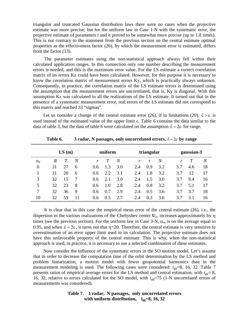
Let us consider a change of the central estimate error (26), if in limitations (20), ε > ε is used instead of the estimated value of the upper limit ε. Table 6 contains the data similar to the data of table 3, but the data of table 6 were calculated on the assumption ε = 2ε for range.

Table 6. 3 radar, N passages, only uncorrelated errors, ε = 2ε by range

LS (m) uniform triangular gaussian-3

nd R T N r T N r t N r T N 0 31 27 6 0.6 1.3 3.0 2.4 0.9 3.2 3.7 4.6 18 1 31 20 6 0.6 2.2 3.1 2.4 1.8 3.2 3.7 12 17 3 32 15 7 0.6 2.1 3.0 2.4 1.5 3.0 3.7 9.4 16 5 32 23 8 0.6 1.0 2.8 2.4 0.8 3.2 3.7 5.1 17 7 32 36 9 0.6 0.7 2.9 2.4 0.5 3.6 3.7 3.7 18 10 32 59 11 0.6 0.5 2.7 2.4 0.3 3.6 3.7 3.1 16

It is clear that in this case the empirical mean error of the central estimate (26), i.e., the

dispersion in the various realizations of the Chebyshev center Uz, increases approximately by η times (see the previous section). For the uniform law in Case 3-N, αm is on the average equal to 0.95, and when ε = 2ε , it turns out that η=20. Therefore, the central estimate is very sensitive to overestimation of an error upper limit used in its calculation. The projective estimate does not have this unfavorable property of the central estimate. This is why, when the non-statistical approach is used, in practice, it is necessary to use a selected combination of these estimates.

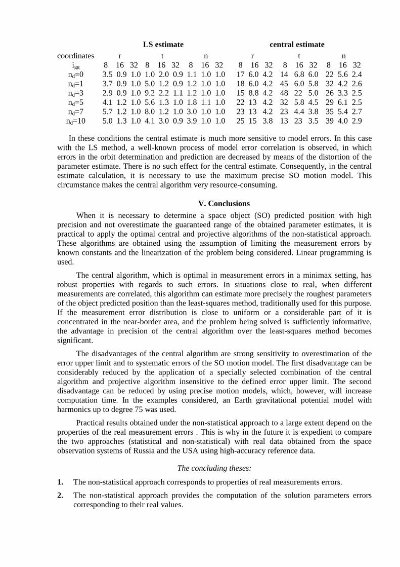
Now consider the influence of the systematic errors in the SO motion model. Let’s assume that in order to decrease the computation time of the orbit determination by the LS method and problem linearization, a motion model with fewer geopotential harmonics than in the measurement modeling is used. The following cases were considered: igg=8, 16, 32. Table 7 presents ratios of empirical average errors for the LS method and central estimation, with igg= 8, 16, 32, relative to errors calculated for the SO model, with igg=75 (1-N uncorrelated errors of measurements was considered).

Table 7. 1 radar, N passages, only uncorrelated errors with uniform distribution, igg=8, 16, 32

LS estimate central estimate coordinates r t n r t n

igg 8 16 32 8 16 32 8 16 32 8 16 32 8 16 32 8 16 32 nd=0 3.5 0.9 1.0 1.0 2.0 0.9 1.1 1.0 1.0 17 6.0 4.2 14 6.8 6.0 22 5.6 2.4 nd=1 3.7 0.9 1.0 5.0 1.2 0.9 1.2 1.0 1.0 18 6.0 4.2 45 6.0 5.8 32 4.2 2.6 nd=3 2.9 0.9 1.0 9.2 2.2 1.1 1.2 1.0 1.0 15 8.8 4.2 48 22 5.0 26 3.3 2.5 nd=5 4.1 1.2 1.0 5.6 1.3 1.0 1.8 1.1 1.0 22 13 4.2 32 5.8 4.5 29 6.1 2.5 nd=7 5.7 1.2 1.0 8.0 1.2 1.0 3.0 1.0 1.0 23 13 4.2 23 4.4 3.8 35 5.4 2.7 nd=10 5.0 1.3 1.0 4.1 3.0 0.9 3.9 1.0 1.0 25 15 3.8 13 23 3.5 39 4.0 2.9

In these conditions the central estimate is much more sensitive to model errors. In this case with the LS method, a well-known process of model error correlation is observed, in which errors in the orbit determination and prediction are decreased by means of the distortion of the parameter estimate. There is no such effect for the central estimate. Consequently, in the central estimate calculation, it is necessary to use the maximum precise SO motion model. This circumstance makes the central algorithm very resource-consuming.

V. Conclusions

When it is necessary to determine a space object (SO) predicted position with high precision and not overestimate the guaranteed range of the obtained parameter estimates, it is practical to apply the optimal central and projective algorithms of the non-statistical approach. These algorithms are obtained using the assumption of limiting the measurement errors by known constants and the linearization of the problem being considered. Linear programming is used.

The central algorithm, which is optimal in measurement errors in a minimax setting, has robust properties with regards to such errors. In situations close to real, when different measurements are correlated, this algorithm can estimate more precisely the roughest parameters of the object predicted position than the least-squares method, traditionally used for this purpose. If the measurement error distribution is close to uniform or a considerable part of it is concentrated in the near-border area, and the problem being solved is sufficiently informative, the advantage in precision of the central algorithm over the least-squares method becomes significant.

The disadvantages of the central algorithm are strong sensitivity to overestimation of the error upper limit and to systematic errors of the SO motion model. The first disadvantage can be considerably reduced by the application of a specially selected combination of the central algorithm and projective algorithm insensitive to the defined error upper limit. The second disadvantage can be reduced by using precise motion models, which, however, will increase computation time. In the examples considered, an Earth gravitational potential model with harmonics up to degree 75 was used.

Practical results obtained under the non-statistical approach to a large extent depend on the properties of the real measurement errors . This is why in the future it is expedient to compare the two approaches (statistical and non-statistical) with real data obtained from the space observation systems of Russia and the USA using high-accuracy reference data.

The concluding theses:

1. The non-statistical approach corresponds to properties of real measurements errors. 2. The non-statistical approach provides the computation of the solution parameters errors

corresponding to their real values.

3. The interpolated algorithms of the non-statistical approach have the property of adaptation to real measurements errors.

4. The estimation of solution parameters in interpolated algorithms turns out more precisely and an advantage in accuracy, in comparison with the method LS, more when the big part of the errors is concentrated in the near-border area.

5. When the problem is more informative, the central algorithm works better than the LS.

6. The correlations in measurement errors worsens the quality of the solution parameters estimation in central algorithm less than for method LS.

7. The projected algorithm is not critical to the accuracy of the knowledge of the errors upper limit. The central algorithm has no such feature. The projected algorithm can lose in accuracy to the central algorithm no more than 2 times.

8. The central and projected algorithms are more critical to the methodical errors of the SO movement model, than the LS-method.

WHEN AND HOW TO PUT ALGORITHMS OF NOT STATISTICAL APPROACH INTO PRACTICE? THE ANSWER TO THIS QUESTION DEPENDS ON ERROR CHARACTERISTICS OF REAL MEASURING TOOLS

References [1.] Khutorovsky Z.N., “Satellite Catalog Maintenance”, Space Research, vol. 31, issue. 4,

pp. 101-114, 1993. [2.] Dicky, V., Khutorovsky Z., Kuricshah A., Menshikov A., Nazirov, R, Pitsyck, A.,

Veniaminov, S. and Yurasov, V., “The Russian Space Surveillance and Some Aspects of Spaceflight Safety,” Adv. Space Res, Vol. 14, № 8, pp. 8(21)-8(31), 1993.

[3.] Khutorovsky Z.N., Boikov V.F., Pylaev L.N., “Low-Perigee Satellite Cataloque Maintenance,” Near-Earth Astronomy (Space Debris), Russian Academy of Science, Institute of Astronomy, Moscow, 1998, pp. 34-101.

[4.] Khutorovsky Z.N., Boikov V.F., Kamensky S.Yu., “Direct Method for the Analysis of Collision Probabilities of Artificial Space Objects in LEO: Techniques, Results and Application,” Proc. of the First European Conference on Space Debris, Darmstadt, Germany, April 1993, pp.491-508.

[5.] Maui Optical and Space Surveillance Technologies Conference, Sept. 1-4, USA, Maui, Hawaii, 2009.

[6.] Khutorovsky Z.N., “Robust and Adaptive Techniques Used for Maintenance of the Catalog of LEO Satellites,” Proc. of the Fifth US/Russian Space Surveillance Workshop, Saint-Petersburg, 24-27 Sept., 2003.

[7.] Lidov M.L., “On Prior Estimates of Parameter Determination Accuracy by Least-Squares Method,” Space Research, 2, # 5, 1962, p. 713-717.

[8.] Elyasberg P.E., Bakhshiyan B.Ts., “Determination of Space Object Flight Trajectory in the Absence of Information on Measurement Error Distribution Law,” Space Research, 7, # 1, 1969, p. 18-27.

[9.] Shekhovtsev A.I., “Measurement Procession Method with Limited Information on the Law of Distribution of Their Errors,” Space Craft Motion Determination, Nauka, Moscow, 1975, p. 131.

[10.] Kotov E.O., “On the Problem of Satellite Orbit Determination with Limited Measurement Errors,” Space Research, 19, # 4, 1981, p. 513-517.

[11.] Traub J.F. and Wozniakowsky H., A General Theory of Optimal Algorithms, Academic Press, New-York, 1980.

[12.] Milanese M., Tempo R., “Optimal Algorithms Theory for Robust Estimation and Prediction,” IEEE Trans. on Automatic Control, vol. AC-30, № 8, August 1985, pp. 730-738.

[13.] Kacewicz B.Z., Milanese M., Tempo R., Vicino A., “Optimality of Central and Projection Algorithms for Bounded Uncertainty,” System Control Letters, vol. 8, 1986, pp. 161-171.

[14.] Milanese M., Tempo R., Vicino A., “Strongly Optimal Algorithms and Optimal Information in Estimation Problems,” Journal of Complexity, 2, 1986, pp. 78-94.

[15.] Tempo R. and Wasilkowski G.W., “Maximum likelihood estimators and worst case optimal algorithms for system identification,” System Control Letters, vol. 10, 1988, pp. 265-270.

[16.] Cramer H., Methods of Mathematical Statistics, Princeton University Press, Princeton, New York, 1946.

[17.] Grenander U., Rosenblatt M., Statistical Analysis of Stationary Time Series, Uppsala, 1956.

[18.] Poljak B.T. and Tsypkin J.Z., “Robust Identification,” Automatica, 16 (1980), pp. 53-63. [19.] Lemoine F.G. et al., The Development of the Joint NASA GSFC and NIMA Geopotential

Model EGM-96, NASA Goddard Space Flight Center, NASA/TP-1998-206861, July 1998.

[20.] Yudin D.B., Goldstein E.G., Linear Programming, Fizmatgiz, 1963.

Figure 1. Realizations of LS and central estimations for model m=2

(distribution of error measurements: Gauss truncated of level 3σ, n=100)

Figure 2. Realizations of LS and central estimations for model m=2

(distribution of error measurements: triangle, n=100)

Figure 3. Realizations of LS and central estimations for model m=2

(distribution of error measurements: uniform, n=100)