Brief Study of Linear Driven Damped Oscillator

Subhajit Mishra4th year, DPS, IISER Kolkata

(Dated: November 12, 2016)

In this article, I have briefly described the Linear Damped Driven Harmonic Oscillation. Thecomplete solution for the system is derived. The steady state fact is used to derive the expressionsfor amplitude, average energy and power of the system. For every theoretical predictions (like,solution, amplitude, energy) a graphical correspondence is given and uses of SHO as detectors andattenuators are described briefly.

I. INTRODUCTION

Linear Harmonic Oscillator is a well known system inphysics. It is the only problem in physics which is ex-actly solvable numerically and analytically. I have usedthe equation of Driven Damped Harmonic Oscillator todescribe some of the phenomenon of the system.

The force I have taken here is sinusoidal and only timedependent. Theoretically it can be any function of spaceand time (f = f(~r, t)). But the simple method can begeneralized very easily! Because of Fourier Series and Su-perposition Principle. We know that any periodic func-tion can be expanded as the sum of sine and cosine.

f(t) =

+∞∑n=−∞

Cneint

If a function is not periodic we can simply make it peri-odic and apply Fourier series. So, theoretically the simpleforce is enough to describe a general system.

For a linear simple harmonic oscillator total energy isalways conserved. But for a Driven Damped oscillatorin the steady state energy is not conserved within thesystem, due to the supply of external force. Since, inthe steady state there is no damping in each cycle en-ergy increases. One might say that these are breakingenergy conservation rule. But the catch is that firstly, itis not an isolated system and secondly, one can say in theother way that: though energy is not conserved withinthe system, it is conserved within the universe. Becausethe external agency is losing some amount of energy tosupply it to the system. Thus net energy of the universeremains conserved. We will see that the rate of energyloss by the system is equal to the rate of energy gain.

Graphs are very useful for understanding a system. Ihave provided few graphs and described the nature of thegraphs which is undoubtedly consistent with the theories.

One of the application of simple harmonic oscillators isto act as detectors as well as attenuators. These followsdirectly from the amplitude graph (FIG: 13). Since noisecancellation is essential in signal processing, it is veryuseful and has immense application in data analysis.

II. SIMPLE DRIVEN DAMPED OSCILLATOR

The general equation of motion of a simple drivendamped oscillator is given by

x+ 2γx+ ω20x = f(t) (1)

where x is the amplitude measured from equilibrium po-sition, γ > 0 is the damping constant, ω0 is the naturalfrequency of simple harmonic oscillator and f(t) is thedriven force term.

For the sinusoidal for equation of motion is

x+ 2γx+ ω20x = f0 cos(ωt) (2)

Let the solution of the homogeneous part is xh. Thehomogeneous equation is,

xh + 2γxh + ω20xh = 0 (3)

Taking the solution of the form xh = Aeλt, we get thecharacteristic polynomial P (λ) = λ2 + 2γλ + ω2

0 = 0,which has the following roots,

λ± = −γ ± σ

where σ =√γ2 − ω2

0 .Solutions to the homogeneous part are,

• xh = e−γt(A1 cosh(σt) + A2 sinh(σt)), for over-damped (γ2 > ω2

0).

FIG. 1. Over damped Oscillator, γ = 5, ω0 = 2

2

• xh = (A+Bt)e−γt, for critically damped (γ2 = ω20).

FIG. 2. Critically Damped Oscillator, γ = ω0 = 5

• xh = e−γt(A3 cos(σt) + A4 sin(σt)), for under-damped (γ2 < ω2

0).

FIG. 3. Under Damped Oscillator, γ = 0.8, ω0 = 2

The constants can be determined by initial conditions.To look for the solution of the in-homogeneous part,

we rewrite (2) as:

z + 2γz + ω20z = f0e

iωt (4)

where xp = Re[z] and f0 cos(ωt) = Re[f0eiωt].

Now putting z = z0eiωt into (4) we get,

(−ω2 + i2γω + ω20)z0e

iωt = f0eiωt (5)

⇒ z0 =f0

−ω2 + i2γω + ω20

(6)

Since z0 ∈ C, we can write z0 = |z0| eiφ with|z0| , φ ∈ R.From (6) we calculate,

|z0| =f0√

(ω20 − ω2)2 + 4γ2ω2

(7)

and the phase

φ = tan−1

(2γω

ω20 − ω2

)(8)

The particular solution is given by,

xp = Re[z] = |z0| cos(ωt+ φ). (9)

The general solution of the Driven Damped Oscillatoris therefore, x(t) = xh(t) + xp(t),

x(t) = e−γt(A3 cos(σt) +A4 sin(σt)) +|z0| cos(ωt+ φ)(10)

Since xh(t) contains e−γt, it rapidly falls down to zeroas t → ∞. For this reason, xh is called transient termand xp is called steady-state term.

FIG. 4. x(t) vs t plot of Driven Damped Oscillator. Note thatas predicted by the theory after sometime the transient solu-tion dies down and we are left with only steady state solution.

In the case of, Damped Oscillator (i.e., when theexternal force (f0) is zero), from (6), (7) and (10) we seethat the complete solution is:

x(t) = e−γt(A3 cos(σt) +A4 sin(σt)) (11)

A. Amplitude analysis of Driven DampedHarmonic Oscillator

At steady state, amplitude of the system is given byEq(7) and I call it A(ω). Therefore,

A(ω) =f0√

(ω20 − ω2)2 + 4γ2ω2

(12)

If ω is given and we want to calculate the value of ω0

at which A(ω) is maximum, we have to differentiate Eq(17) w.r.t ω0. And by doing that we get

ω0 = ω (13)

3

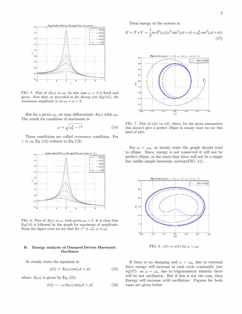
FIG. 5. Plot of A(ω) vs ω0. In this case ω = 3 is fixed andgiven. Note that, as described in the theory (see Eq(13)), themaximum amplitude is at ω0 = ω = 3.

But for a given ω0, we may differentiate A(ω) with ω0.The result for condition of maximum is

ω =√ω20 − γ2 (14)

These conditions are called resonance condition. Forγ � ω0 Eq (14) reduces to Eq (13).

FIG. 6. Plot of A(ω) vs ω, with given ω0 = 3. It is clear thatEq(14) is followed by the graph for maximum of amplitude.From the figure even we see that for γ2 � ω2

0 , ω ≈ ω0

B. Energy analysis of Damped Driven HarmonicOscillator

At steady state the equation is:

x(t) = A(ω) cos(ωt+ φ) (15)

where A(ω) is given by Eq (12).

x(t) = −ωA(ω) sin(ωt+ φ) (16)

Total energy of the system is:

E = T+V =1

2mA2(ω)(ω2 sin2(ωt+φ)+ω2

0 cos2(ωt+φ))

(17)

FIG. 7. Plot of v(t) vs x(t). Since, for the given parametersthis doesn’t give a perfect ellipse in steady state we see thiskind of plot.

For ω = ω0, at steady state the graph should tendto ellipse. Since, energy is not conserved it will not beperfect ellipse, in the sense that there will not be a singleline unlike simple harmonic motion(FIG. 11).

FIG. 8. v(t) vs x(t) for ω = ω0

If there is no damping and ω = ω0, due to externalforce energy will increase in each cycle constantly (seeeq(17): as ω = ω0, due to trigonometric identity therewill be not oscillation. But if this is not the case, thenEnergy will increase with oscillation. Figures for bothcases are given below:

4

FIG. 9. v(t) vs x(t) with ω = ω0

FIG. 10. v(t) vs x(t) with ω 6= ω0

For no force and no damping case, energy phase-spaceplot will be a perfect ellipse.

FIG. 11. phase space plot for f0 = 0 = γ

The average energy is:

〈E〉 =1

4mA2(ω)(ω2 + ω2

0) (18)

Since, 〈sin2 θ〉 = 〈cos2 θ〉 = 12 . Putting the expression

of A(ω) into Ez (18), we get the full expression of total

average energy:

〈E〉 =f204m

ω2 + ω20

(ω20 − ω2)2 + 4γ2ω2

(19)

Now for very weak damping (γ2 � ω20) ω ≈ ω0: There-

fore,

〈E〉 =f208m

1

(ω0 − ω)2 + γ2(20)

Since, at ω ≈ ω0: ω2 + ω20 ≈ 2ω2

0 and ω20 − ω2 = (ω0 +

ω)(ω0−ω) ≈ 2ω0(ω0−ω) The average energy is maximumwhen ω = ω0:

〈E〉max =f20

8mγ2(21)

FIG. 12. Plot of E(t) vs t, with γ2 � ω20 = ω2. From the

figure it is evident that after reaching steady state the averageenergy becomes constant and is nearly equal to (21). Thenumerical value of 〈Emax〉 for the given parameters is ≈ 12.5

By looking at the Eq (19) we see that for fix f0, ω, ω0,m and γ, the average energy is same at all t.

Proposition: Average power dissipation by dampingforce gets balanced by average power supplied by drivingforce.

The proof is given below.

1. Power dissipation by Damping Force:

Pdamping = Fdampingv = (−Γx)x where Γ = mγ.Putting x from Eq(16), we get:

Pdamping = −Γ(ωA)2 sin2(ωt+ φ) (22)

So, the average power dissipation is given by:

〈Pdamping〉 = −1

2Γ(ωA2) (23)

5

2. Power supplied by Driving Force:

Pdriving = Fdrivingx = f0 cosωt x. Putting x and usingthe formula for sin(A+B) we get:

Pdriving = −f0ωA cosωt(sinωt cosφ+ cosωt sinφ) (24)

Taking time average we get:

〈Pdriving〉 = −1

2f0ωA sinφ (25)

From Eq(8), by calculating sinφ, we get:

sinφ =2γωA

f0(26)

Putting (26) back into (27) and simplifying we get:

〈Pdriving〉 =1

2(ωA)2 (27)

Therefore, 〈Pdamping〉+ 〈Pdriving〉 = 0 and we proved theproposition.

III. USING SHO MOTION AS DETECTORSAND ATTENUATORS

Harmonic motion can be used as detectors. It can beexplained by looking at the amplitude graph.

FIG. 13. Amplitude Graph

From the above figure we can see that there are mainlythree regions in the amplitude graph. These are: forcesregion, resonance region and damping region.

The forces region is more or less constant. For anystable detection we use this region. At resonance region,

we can pin point the frequency of the signal. We can useuse damping region into data analysis, since most of thenoises die down in that region.

A simple use of SHO as attenuators can befound at LIGO. Where it is used to remove seis-mic noise, if the required frequency is way abovethe resonance frequency i.e., in the damping re-gion.

IV. CONCLUSION

There are many topics and phenomenons regardingDriven Oscillators, I have described few of them. Fromthe plots we indeed see that the theoretical calculationdramatically matches with the numerical solutions. FromFIG:9 we indeed see that energy of a driven oscillator isnot conserved. But as discussed earlier it does not vi-olate conservation of energy. And we also see from theplot that energy of a simple harmonic oscillator is con-served, which we expect. SHM is very useful in physicsbecause, more or less every system can be modelled usingSHM and as stated earlier it is the only system which isexactly solvable.

I have generated the plots using python.

V. REFERENCES

[1] David Morin, Oscillations, Harvard University,http://www.people.fas.harvard.edu/~djmorin/waves/oscillations.pdf.

[2] N. K Bajaj, The Physics of Waves and Oscillations,McGrawHillEducation, 1998.

[3] Dr. Eric Ayars, Computational Physics WithPython, Aug’18, 2013.

[4]http://docs.scipy.org/doc/scipy/reference/generated/scipy.integrate.odeint.html#scipy.integrate.odeint

[5] http://ocw.mit.edu/courses/mathematics/18-03sc-differential-equations-fall-2011/unit-ii-second-order-constant-coefficient-linear-equations/damped-harmonic-oscillators/MIT18_03SCF11_s13_2text.pdf

[6]R. K. Nayak, Simple Harmonic Motion and Gravi-tational Wave Detection