b.sc., shandong university, china, 1996 a thesis submitted
TRANSCRIPT
SHIFTED FREQUENCY ANALYSIS FOR EMTPSIMULATION OF POWER SYSTEM DYNAMICS
by
Peng Zhang
B.Sc., Shandong University, China, 1996M.Sc., Shandong University, China, 1999
A THESIS SUBMITTED IN PARTIAL FULFILLMENT OFTHE REQUIREMENTS FOR THE DEGREE OF
DOCTOR OF PHILOSOPHY
in
The Faculty of Graduate Studies
(Electrical and Computer Engineering)
THE UNIVERSITY OF BRITISH COLUMBIA(Vancouver)
March 2009
© Peng Zhang, 2009

Abstract
Electromagnetic Transients Program (EMTP) simulators are being widely used in power
system dynamics studies. However, their capability in real time simulation of power systems is
compromised due to the small time step required resulting in slow simulation speeds.
This thesis proposes a Shifted Frequency Analysis (SFA) theory to accelerate EMTP
solutions for simulation of power system operational dynamics. A main advantage of the SFA is
that it allows the use of large time steps in the EMTP solution environment to accurately
simulate dynamic frequencies within a band centered around the fundamental frequency.
The thesis presents a new synchronous machine model based on the SFA theory, which
uses dynamic phasor variables rather than instantaneous time domain variables. Apart from using
complex numbers, discrete-time SFA synchronous machine models have the same form as the
standard EMTP models. Dynamic phasors provide envelopes of the time domain waveforms and
can be accurately transformed back to instantaneous time values. When the frequency spectra of
the signals are close to the fundamental power frequency, the SFA model allows the use of large
time steps without sacrificing accuracy. Speedups of more than fifty times over the traditional
EMTP synchronous machine model were obtained for a case of mechanical torque step changes.
This thesis also extends the SFA method to model induction machines in the EMTP. By
analyzing the relationship between rotor and stator physical variables, a phase-coordinate model
with lower number of equations is first derived. Based on this, a SFA model is proposed as a
general purpose model capable of simulating both fast transients and slow dynamics in induction
machines. Case study results show that the SFA model is in excess of seventy times faster than
the phase-coordinate EMTP model when simulating the slow dynamics.
In order to realize the advantage of SFA models in the context of the simulation of the
complete electrical network, a dynamic-phasor-based EMTP simulation tool has been developed.
11

Table of Contents
Abstract ii
Table of Contents iii
List of Tables vi
List of Figures vii
Acknowledgements xi
Chapter 1 Introduction 1
1.1 Background 1
1.2 Motivation 3
1.3 Contributions 5
Chapter 2 Shifted Frequency Analysis 6
2.1 Analytic Signal and Hubert Transform 6
2.1 .1 Shifted Frequency Analysis 7
2.2 SFA-Based Network Component Models 10
2.2.1 Equivalent Circuits for RLC in the Shifted Frequency Domain 11
2.2.2 Options between Complex Arithmetic and Real Arithmetic 15
2.2.3 Transformer Model in the Shifted Frequency Domain 17
2.2.4 Load Models 20
2.3 Numerical Accuracy Analysis 27
Chapter 3 Synchronous Machine Modelling Based on Shifted Frequency Analysis 33
3.1 Introduction 33
3.2 Voltage-behind-Reactance Synchronous Machine Model 33
111

Table of Contents
3.3 Synchronous Machine Modelling with SFA .38
3.3.1 Synchronous Machine Model Based on SFA 38
3.3.2 Discrete Time Model 39
3.3.3 Note on the Cylindrical-Rotor Machine Model 45
3.4 Simulation Results 47
3.4 Summary 57
Chapter 4 Induction Machine Modelling Based on Shifted Frequency Analysis 58
4.1 Introduction 58
4.2 Equivalent-Reduction Approach to Induction Machine Modelling in EMTP. 59
4.2.1 Equivalent-Reduction (ER) to Stator Quantities 60
4.2.2 Induction Machine Modelling Based on ER Technique 60
4.2.3 Simulation Results 65
4.3 Induction Machine Modelling with SFA 71
4.3.1 Induction Machine Modelling Based on SFA 71
4.3.2 Discrete Time Model 72
4.3.3 Simulation Results 73
4.4 Summary 80
Chapter 5 EMTP Implementation 81
5.1 Introduction 81
5.2 Program Structure 82
5.3 Test Cases 86
Chapter 6 Conclusions 102
6.1 Summary of Contributions 102
6.2 Future Research 103
Bibliography 105
Appendix A Machine Parameters 111
A. 1 Synchronous Machine Parameters 111
iv

Table of Contents
A.2 Induction Machine Parameters.112
Appendix B Voltage behind Reactance Induction Machine Model 113
B. 1 Voltage Behind Reactance Model of Induction Machine 113
B. 2 Discrete Time VBR Model 116
B. 3 Free Acceleration Simulation of a 3-hp Induction Machine 118
B. 4 Dynamic Performance of Induction Machine during Mechanical Torque
Changes 118
Appendix C Test Case Data 123
V

List of Tables
Table 2.1 Load Increased with the Time 23
Table 3.1 CPU Times for 4s Simulation in Case C 50
Table 3.2 Accuracy Comparison between SFA Model and VBR EMTP Model in Case C 56
Table 4.1 CPU Times for Simulations 71
Table 4.2 CPU Times for Simulations 75
Table 4.3 CPU Times for Simulations 79
vi

List of Figures
Figure 2.1(a) M Coupled Inductances; (b) EMTP Equivalent Circuit; (c) SFA Equivalent
Circuit 9
Figure 2.2 (a) Series Connection of M-phase R and L; (b) EMTP Equivalent Circuit; (c) SFA
Equivalent Circuit 13
Figure 2.3 Linear Test Case 13
Figure 2.4 Current Flowing through Branch 1-2 (At = ims) 14
Figure 2.5 Linear Time Varying Test Case 14
Figure 2.6 Voltage across the Time Varying Inductance (At 0.5 ms) 15
Figure 2.7 Single-Phase Two-Winding Transformer 18
Figure 2.8 Secondary Winding Voltage (At = 50 ms) 20
Figure 2.9 Equivalent Circuit for the Exponential Load 21
Figure 2.10 Two Node Test Case 21
Figure 2.11 Simulation Results of the Node Voltage (a) SFA Solution (At = 10 ms) (b)
EMTP Solution (At = 0.5 ms) 22
Figure 2.12 Simulation Results of Voltage Collapse (a) SFA Solution (At = 10 ms) (b) EMTP
Solution (At = 0.5 ms) 22
Figure 2.13 SFA Simulation Results of the Voltage Collapse Process (At = 10 ms) 23
Figure 2.14 Steady State Equivalent Circuit 24
Figure 2.15 Discrete Time Equivalent Circuit 24
Figure 2.16 Motor Test Case 26
Figure 2.17 Induction Motor Terminal Voltage (At = 5 ms) 27
Figure 2.18 Real Power Absorbed by the Induction Motor (At = 5 ms) 27
Figure 2.19 Slip of Induction Motor (At = 5 ms) 27
Figure 2.20 Equivalent Circuit Le for Backward Euler and Forward Euler (L=1; & 1 cycle,
3 cycles, 5 cycles) 30
Figure 2.21 Accuracy of integration rules (a) Magnitude (b) Phase 31
vii

List of Figures
Figure 3.1 Salient-Pole Synchronous Machine and Its Windings 34
Figure 3.2 SFA Equivalent Circuit of a Synchronous Generator 43
Figure 3.3 Simulation Results with the SFA Model for Field Voltage and Mechanical Torque
Changes(At=7ms) 51
Figure 3.4 Simulation Results with the SFA Model for a Three Phase Fault (At 0.5 ms): A
Stable Case (fault removed at 1 .4s) 52
Figure 3.5 Simulation Results with the SFA Model for a Three Phase Fault (At = 0.5 ms): An
Unstable Case (fault removed at 1 .5s) 53
Figure 3.6 Simulation Results with the SFA Model for a Three Phase Fault (At = 0.5 ms):
Zoomed-in View of a Portion of Results in Figure 3. 5 54
Figure 3.7 Simulation Results with the SFA Model for a Single-Phase-to-Ground Fault (At =
0.5 ms) 54
Figure 3.8 Simulation Results by SFA: Phase A Stator Current 55
Figure 3.9 Simulation Results by SFA: Zoomed-in View of Phase A Stator Current 55
Figure 3.10 Simulation Results by SFA: Field Current 55
Figure 3.11 Simulation Results by SFA: Electromagnetic Torque 56
Figure 3.12 Simulation Results by SFA: Rotor Speed 56
Figure 3.13 Time Domain Results Using the VBR Model (At = 10 ms) 57
Figure 4.1 Torque-Speed Characteristics during Free Acceleration of a 2250-hp Induction
Machine (At = 500 us) 66
Figure 4.2 Dynamic Performance of a 3-hp Induction Machine during Free Acceleration (At
=500ts) 67
Figure 4.3 Dynamic Performance of a 3-hp Induction Machine during Step Changes in Load
Torque (At = 500 jis) 68
Figure 4.4 Simulation Results for a 3-Phase Fault at the Terminals of a 2250-hp Induction
Machine (At = 100 us) 69
Figure 4.5 Simulation Results for a 3-Phase Fault with Different Time Steps 70
Figure 4.6 SFA Equivalent Circuit of an Induction Machine 73
Figure 4.7 Stator Current during Free Acceleration of a 2250-hp Induction Machine (At =
500 us) 74
viii
List of Figures
Figure 4.8 Dynamic Performance of a 3-hp Induction Machine during Free Acceleration (At
=500.is) 75
Figure 4.9 Dynamic Performance of a 3-hp Induction Machine during Step Changes in Load
Torque (RE At = 0.5 ms, SFA At =5 ms) 76
Figure 4.10 Simulation Results for a 3-Phase Fault at the Terminals of a 2250-hp Induction
Machine (At = 500 ps) 77
Figure 4.11 Simulation Results by SFA 78
Figure 4.12 Time Domain Results from an EMTP Algorithm Implemented in MATLAB 79
Figure 5.1 Schematic Structure for the EMTP Dynamic Phasor Simulation Tool 83
Figure 5.2 The H Transmission Line Model 84
Figure 5.3 Contributions of the H-Circuit Transmission Line Model to the Nodal Admittance
Matrix 85
Figure 5.4 The MATLAB Code for Inserting H-Circuit Transmission Line Model into G
Matrix 86
Figure 5.5 Flow Chart for Dynamic-Phasor-Based EMTP Simulator 87
Figure 5.6 One-line Diagram of a Radial Test System 87
Figure 5.7 Phase A Voltage at the Load Node (At = 5 ms) 88
Figure 5.8 Zoomed-in View of Phase A Voltage at the Load Node (At = 5 ms) 88
Figure 5.9 Phase B Voltage at the Load Node (At = 5 ms) 88
Figure 5.10 Zoomed-in View of Phase B Voltage at the Load Node (At = 5 ms) 89
Figure 5.11 Phase C Voltage at the Load Node (At = 5 ms) 89
Figure 5.12 Zoomed-in View of Phase C Voltage at the Load Node (At = 5 ms) 89
Figure 5.13 One Line Diagram for the Test Feeder 90
Figure 5.14 Phase A Voltage at the Induction Machine Node (At = 1 ms) 91
Figure 5.15 Zoomed-in View of Phase A Voltage at the Induction Machine Node (At = 1 ms) ..91
Figure 5.16 Phase B Voltage at Load Node 6 (At = 1 ms) 91
Figure 5.17 Zoomed-in View of Phase B Voltage at Load Node 6 (At = 1 ms) 92
Figure 5.18 Phase C Voltage at Node 1 (At = 1 ms) 92
Figure 5.19 The First Benchmark Network for Subsynchronous Resonance Studies 93
Figure 5.20 Generator Terminal Voltage: Phase A (At = 1 ms) 94
Figure 5.21 Transformer High Side (Bus A) Voltage: Phase A (At = 1 ms) 95
ix

List of Figures
Figure 5.22 Voltage across Series Capacitor: Phase A (At = 1 ms) 95
Figure 5.23 Infinite Bus (Bus B) Voltage: Phase A (At = 1 ms) 96
Figure 5.24 The Second Benchmark Network for Subsynchronous Resonance Studies 98
Figure 5.25 Generator Terminal Voltages: Phase A (At = 1 ms) 99
Figure 5.26 Voltage across Series Capacitor: Phase A (At = 1 ms) 99
Figure 5.27 Transformer High Side (Bus 2) Voltage: Phase A (At = 1 ms) 100
Figure 5.28 Infinite Bus (Bus 1) Voltage: Phase A (At = 1 ms) 100
Figure B. 1 Free Acceleration Characteristics in Stationary Reference Frame 119
Figure B.2 Free Acceleration Characteristics in Rotor Reference Frame 120
Figure B.3 Free Acceleration Characteristics in Synchronous Reference Frame 121
Figure B.4 Dynamic Performance of a 3-hps Induction Machine during Step Changes in
Load Torque 122
x

Acknowledgements
I would like to express my deep gratitude to my supervisors Dr. José R. MartI and Dr.
Hermann W. Dommel. My admiration for their great achievements and contributions was the
reason why I decided to study with them in Canada. I want to thank Dr. MartI for his consistent
guidance and financial support during my study at UBC. The inspiration and warm personality of
Dr. MartI and Dr. Dommel have won the author’s highest respect and love.
I sincerely thank my friends and colleagues at UBC and British Columbia Transmission
Corporation for their encouragement and understanding.
My wife Helen, my parents Yihua and Guangfu, are sources of unconditional love and
support since the beginning of this project. They are entitled to more thanks than can be
expressed here. My parents-in-law Guier and Jingxiang, my brother Kun, my brother-in-law
Hailu, my sister-in-law Haiyang are also important members of the team that supports me
permanently. To all my family, from the depths of my heart, thank you.
xi

Chapter 1 Introduction
Chapter 1
Introduction
1.1 Background
Although a power system blackout is a low-probability event, whenever it happens, its
impact on the power system and the society is catastrophic. A typical example is the Aug. 14,
2003 Blackout in the USA and Canada, which caused a total loss of 62,000 MW of loads and
tripping of 531 generators [1]. Fifty million people were affected by this system collapse. During
the next two years, twelve major blackouts happened in Europe, Asia and North America. A
recent blackout happened in Los Angeles on September 12, 2005 affecting millions in California.
In today’s deregulated electricity market environment, power system planning and
operations are largely driven by economic motivations, without sufficient investments in new
generation and transmission equipments. This might have contributed to the higher frequency of
blackouts in recent years [2]. Because of aging infrastructures operating under stressed
conditions, power system stability, including transient stability, voltage stability, and inter-area
oscillations have become a major concern in the North American power grid.
Traditionally in power system studies a number of simplifying assumptions are made to
analyze different types of stability problems with specific tools [3]-[5]. For instance, the static
techniques for long-term voltage stability analysis [6] only solve the steady-state (algebraic)
response of the system. Another example is quasi-steady-state (QSS) analysis [7], which neglects
the fast network transients and only considers electromechanical dynamics. Because the time
varying electrical quantities in QSS are represented with phasors, these tools can only capture
snapshots of the system operation ignoring the dynamics between states.
Problems such as voltage stability depend strongly not only on the machine-network
interaction, but also on the interaction between the electrical network and the loads. Moreover,
1

Chapter 1 Introduction
severe disturbances in the system often involve frequency excursions in addition to voltage
excursions [8]. Especially when the power system is approaching critical collapse points, the
QSS or steady-state assumptions can result in inaccurate predictions.
Tools such as the EMTP [9][10] can most closely simulate the real power system
dynamics by continuously tracing the evolution of the system state in arbitrary multi-phase
networks with lumped or distributed parameters. Therefore EMTP-type simulators [11] -[15] are
very appealing to be used for power system stability assessment. These tools, however, require
small discretization steps dictated by the need to trace the instantaneous values of all waveforms.
This makes the EMTP unnecessarily slow to trace phenomena around the 60 Hz fundamental
frequency. As a matter of fact, nowadays one can only simulate small-scale equivalent power
systems on the real-time EMTP simulators [10] [16]. Therefore, efforts should be taken to bridge
the gap between the EMTP-type simulators and a unified power system analysis tool.
Reference [18] aims at combining electromagnetic and electromechanical simulations
[19] by considering both the network and machine differential equations without making QSS
assumptions. However, no efficient solution algorithms are provided in this reference and the
presented machine models are still reduced order models in phasor form. Reference [20]
provides the first systematic method for a unified steady-state and transient power system
analysis tool, by combining dynamic phasor concepts with EMTP simulation. Dynamic phasor
models for transmission lines and linear elements are presented in this reference. However, the
machine model is still based on the dq0 model, which can present numerical stability problems
for large time steps and may not be the most appropriate for a general EMTP-based dynamic
phasor unified theory. Important contributions to dynamic phasor modeling of electric machines
have been presented in [21], [22], [23] based on the approach of the generalized averaging
method [23] which, however, is also an approximate method with higher frequency components
truncated.
In general, it is a challenging topic to correctly, efficiently obtain the time-domain
simulation results in the neighborhood of the fundamental frequency without making QSS or
other simplif4ng assumptions. Hence, the intention of this thesis is to explore an effective way
to combine the EMTP solution and the dynamic phasor concept, to build dynamic phasor models
for power system components, and to develop a general-purpose simulation tool to obtain
dynamic phasor results from EMTP solutions.
2

Chapter 1 Introduction
1.2 Motivation
It is important to have some insight into the power system signals before we can further
develop an efficient and accurate method for power system dynamic simulation.
A conmion observation is that, when a contingency happens, the frequencies in a power
system are usually close to fundamental frequency co3 (60 Hz). That is to say, in the dynamic
situation, the electrical signals in power systems have a fundamental frequency component
modulated by slower events. This fact is analogous to the situation in communication systems
where the carrier frequency is very high and carries on its sidebands the much lower frequency
(e.g., audio or video) information. In communications theory, the carrier frequency is modulated
to send out the information and then demodulated to recover the information at the receiving end
[24]. Typically the carrier in a communication system is a sinusoidally varying signal at some
frequency which is much higher than the frequencies contained in the information or message.
The process of modulation gives the signal a nonzero bandwidth that is usually much smaller
than the carrier frequency. Thus the signal can be regarded as a narrowband process, and can be
accurately modeled as the product of a bandlimited ‘message’ waveform and a sinusoidal carrier.
By this analogy, one can directly draw the conclusion that usually a power system signal u(t)
can be modeled by a narrowband signal which has a small bandwidth around a.
In steady-state AC circuit theory, one uses complex exponentials (i.e. phasors) to
represent real sinusoidal signals with the understanding that the real part of the complex
exponential gives the physical time-domain quantity of the AC signal.
Going beyond the steady-state analysis, the analytic signal of a real function plays the
similar role for a dynamic waveform. In fact, the analytic signal z(t) of a bandpass signal u(t)
can be derived as:
(1.1)
where UQ) is called the dynamic phasor of u(t), zQ) = uQ) + 1H[u(t)], and H[.] denotes the
Hilbert transform [25][26].
The dynamic phasor UQ) is the complex envelope of u(t), and will degenerate to the
phasor U if uQ) becomes a sinusoidal signal in steady state. In fact, the analytic signal of a
steady-state sinusoidal function Acos(a3t+ço) is Be°’ where B = Here the dynamic phasor
3
Chapter 1 Introduction
becomes which is the phasor ofAcos(cot+q).
Similar to the phasor, the dynamic phasors can be transformed back to time domain
waveforms by taking the real part of the analytic signal in (1.1) (proof is shown in Chapter 2)
It can be seen in (1.1) that the spectrum of U(t) is the spectrum of the analytic signal of
u(t) shifted by synchronous angular frequency — o. This can be called the “frequency shifting”
property. If the power network is formulated by using dynamic phasors instead of the
instantaneous time quantities, it is said to be modeled in the shifted frequency domain, as
opposed to the model in the time domain. Similar idea is proposed in reference [27]. The way to
build power system component models and solve the network equations in the shifted frequency
domain is called the Shifted Frequency Analysis (SFA).
A major advantage of the Shifted Frequency Analysis is that it allows the use of large
time steps in the EMTP solution environment to accurately simulate dynamic frequencies within
a band centered around a fundamental frequency. The original system is transformed into a
shifted frequency system where the frequencies around the power frequency (e.g. 60Hz) become
frequencies around dc (0 Hz) [28][29]. Because the time step in EMTP simulations is limited by
the Nyquist frequency, low frequencies in the shifted frequency system imply the feasibility of
using large integration time steps.
By coupling SFA models into an EMTP-type simulator, the shifted system is then
numerically integrated to obtain dynamic phasor solutions, which are more easily understood by
power system operators and planners than instantaneous time domain results. At the same time,
the dynamic phasor results can then be transformed back to time domain waveforms using the
inverse transformation.
EMTP uses the trapezoidal integration rule that is A-stable, reasonably accurate and
simple. The discrete-time nodal equations formed in EMTP are elegant and can preserve the
sparsity of the power system structure. All these features makes EMTP a standard simulation
tool in the power industry that can model the power system at the device level. The goal of this
thesis is to implement the SFA method into EMTP, which is the first practical step for building a
unified power system analysis tool based on the EMTP solution.
4

Chapter 1 Introduction
1.3 Contributions
A two-step strategy is employed in the research of Shifted Frequency Analysis. First, the
SFA-based models for power network components are developed and tested. Second, a general-
purpose SFA-based EMTP tool is built to simulate a power network. The main contributions are
presented in Chapter 2 to Chapter 5 and are briefly summarized as follows.
I. The definition of dyhamic phasor and the theoretical basis of the SFA method are introduced.
The basic procedures for analyzing time functions (signals) in the SFA domain are discussed,
and the numerical accuracy of the discrete-time SFA solution is analyzed. Chapter 2 summarizes
these theoretical works.
II. A few types of power system components are modeled in the SFA domain. Chapter 2
describes the SFA-based models for the linear circuit components, transformer and some load
models such as exponential load and steady state induction motor load.
III. A new efficient synchronous machine model for the simulation of slow system dynamics
using EMTP modelling in the Shifted Frequency Analysis framework is presented in Chapter 3.
Discrete-time SFA synchronous machine models are derived which have a similar form as the
EMTP component models.
IV. In Chapter 4, the SFA method is extended to model the induction machines in EMTP. By
analyzing the relationship between rotor and stator physical variables, a phase-coordinate model
with lower number of equations is first derived. Based on this, a SFA model is proposed as a
general purpose model capable of simulating both fast transients and slow dynamics. Case study
results have confirmed that the SFA induction machine model is a valuable component for real
time EMTP simulations. It is observed that the SFA model is in excess of 70 times faster than the
EMTP phase-coordinate model when simulating dynamics with frequency spectra close to the
fundamental power frequency.
V. A final contribution in this thesis is a dynamic-phasor-based EMTP simulation tool. The
structure of the tool and the test system results are reported in Chapter 5.
5

Chapter 2 Shifted Frequency Analysis
Chapter 2
Shifted Frequency Analysis
2.1 Analytic Signal and Hubert Transform
The Fourier transform F(co) of a real-valued functionf(t) is a Hermitian function, which
means F(—co) = F*(w) in the frequency domain. Thus the F for negative frequencies can be
expressed by F* (complex conjugate of F) for positive ones. This means that the positive
frequency spectra is adequate to represent a real signal, and the negative frequency components
of the Fourier transform can be discarded without loss of information. Now one can construct a
function Fa(0) that contains only the non-negative frequency components of F(co) by defining
Fa(O)) F((D) + sgn(aF(ü) (2.1)
where
1 a)>O
sgn(o)= 0 o=0
—1 o<0
The analytic signalfa(t) is defined to be the inverse Fourier transform Of Fa(CO)
L(t)=f(o0)td
=-- f F(o)e°tdo (2.2)
It is clearly seen thatLQ) is a complex function. If we define the Hubert transform off(t)
as the imaginary part Offa(t), and denote it by H[fQ)] = f(t), thenL(t) can be expressed as
fQ) =JQ) +jfQ) (2.3)
6

Chapter 2 Shifted Frequency Analysis
From equation (2.1) and (2.3) we can get the following Fourier pair
JQ) +jfQ) -> F(o) + sgn(F(w)
F
Because we haveJ(t) F(w) by definition, we can derive that
f(t) -jsgn(co)F(co)
iFUsing the transform pair — -+ —jsgn(co) and taking the inverse Fourier transform of
—jsgn(o).F(a), we can get
H[fQ)]=j(t) = ±*fQ)= --PVfdr (2.4)
Note that the Hubert transform is an improper integral, thus it is calculated using the
Cauchy principal value (see the ‘PV’ in (2.4)), i.e. f(t) iimi[j dr+ A
dr].-A t—r
Obviously, H[f(t)] is real.
The analytic signal has no negative frequency components; moreover, the original real
signal can be converted back from it by simply dropping the imaginary part. The analytic signal
is thus a generalization of the phasor concept. This important implication leads to the shifted
frequency analysis method as is explained in the following section.
2.1.1 Shifted Frequency Analysis
If a power system signal u(t) is a bandpass one, it can then be represented [201 as.
u(t) = u1 (t) cos oit — UQ (t) sin ot (2.5)
where the lowpass signals u1 (t) and UQ (t) are the in-phase and quadrature components of the
bandpass signal, respectively.
The dynamic phasor U(t) for the signal u(t) is defined as
U(t)=uJ(t)+juQ(t)
which is the complex envelope of u(t).
Assume that z(t) is the analytic signal ofu(t), then
z(t)e°’ = {uQ) + jH[u(t)Je0t
7

Chapter 2 Shifted Frequency Analysis
= {u1 (t) cos ot — UQ (t) sin ot + j[1 (t) sin cost + UQ (t) cos
u1(t)+fu0(t) (2.6)
where H[.] denotes the Hubert transform.
Therefore,
U(t) z(t)e°’ (2.7)
Note that the dynamic phasor U(t) will degenerate to the phasor U if u(t) becomes a
sinusoidal signal in steady state.
Equation (2.7) shows that the spectrum of U(t) is the spectrum of the analytic signal of
u(t) shifted by synchronous angular frequency—
co,. This is called “frequency shifting”.
Shifted frequency analysis (SFA) [24] allows the exact simulation of frequencies within a
band centered around a fundamental frequency using large time steps in a discrete-time EMTP
type of solution environment. The original system is transformed into a shifted frequency system
where the frequencies around the power frequency (60Hz or 50Hz) become frequencies around
dc (0 Hz). The shifted system is then solved using an EMTP solution.
The equivalent circuit for network components in the shifted frequency domain can be
derived in three steps:
(i) Create the phase-coordinate differential equations of the component in the normal
unshifted domain;
(ii) Transform phase quantities into dynamic phasor variables according to Equation
(2.7);
(iii) Discretize the dynamic phasor equations using an integration method, e.g. the
trapezoidal rule, and build the equivalent circuit suitable for an EMTP solution.
For instance, the time domain voltage equations for M coupled inductances, shown in
Figure 2.1(a), can be written as
v(t)=tLt) (2.8)
As illustrated in Figure 2.1(b), the standard EMTP equivalent circuit derived with the
trapezoidal rule can be written as
1(t) =R1v(t)— hL (t) (2.9)
where
8

Chapter 2 Shifted Frequency Analysis
RL =- (2.10)
is an MxM matrix of resistances, and
hL(t)=L’v(t — At)At + hL (t — At) (2.11)
is a vector of past histories.
To obtain the SFA equivalent circuit (Figure 2.1(c)), we transform (2.8) using (2.7) to get
V(t)= LdIQ)
+jo3L1(t) (2.12)
where V(t) and 1(t) are the dynamic phasor vectors corresponding to the physical time vectors
v(t) and i(t), respectively.
We can now transform (2.12) to discrete time using, for example, the trapezoidal rule,
1(t) =R1V(t)— HL (t) (2.13)
where the equivalent resistances RL and history terms HL (t) are expressed as
2L (2RL =—+KL (2.14)
4 2.—-—+JO)
At2L1V(t — At) —
HL (t — At) (2.15)
-+jcO
The corresponding SFA equivalent circuit is shown in Figure 2.1(c).
L
p p
(a
RL = 2L/At RL = (2/At+ jco)L
hL(t) HLQ)
(b) (c)
Figure 2.1 (a) M Coupled Inductances; (b) EMTP Equivalent Circuit; (c) SFA Equivalent Circuit
A major advantage of SFA modelling is that since the equivalent circuits are centered
9

Chapter 2 Shifted Frequency Analysis
around 60 Hz (ja)L for the inductances of Figure 2.1), deviations from 60 Hz correspond
numerically to very low frequencies (like deviations from 0 Hz in the unshifted domain) and a
large integration step can be used in the solution. For example, respecting the accuracy limits
imposed by the Nyquist frequency and the distortion introduced by the discretization rule [30],
allowing a 3% error with the trapezoidal rule, the integration step can go, for example, from
about three 60 Hz cycles, 5Oms, for frequency deviations of± 2Hz to as large as is for frequency
deviations of± 0.1Hz. With these time steps, the SFA method provides an effective way to make
the EMTP program a general purpose simulator for power system stability problems.
By applying SFA in an EMTP-type simulator, time varying phasor solutions are obtained,
which can be easily understood by power system operators and planners. At the same time,
detailed waveform results can also be traced back from the SFA results by using the inverse
transformation
u(t) = Re[U(t)e.t 1 (2.16)
Unless specifically noted, in this paper uppercase letters are used to represent dynamic
phasors in the shifted frequency domain, while lowercase letters denote real variables in the time
domain.
2.2 SFA-Based Network Component Models
The component models in the SFA domain are building blocks for a SFA-based network
simulator. In this section, we implement the SFA modeling technique described in Section 2.1.1
and build component models for the linear RLC components, transformer, exponential load and
steady-state induction machine. SFA equivalent circuits for other network components can also
be derived following the procedures in Section 2.1.1. Particularly, two important dynamic
components in the power system, i.e. synchronous machine and induction machine, are modeled
in SFA domain in Chapter 3 and Chapter 4.
10

Chapter 2 Shifted Frequency Analysis
2.2.1 Equivalent Circuits for RLC in the Shifted Frequency Domain
The equivalent circuits for network components in the shifted frequency domain can be
derived by first writing the component equations in the phase domain and then relating phase and
dynamic phasor variables according to the frequency shifting transformation.
A. M-Phase Resistances
The time domain voltage equations for M-Phase resistances are expressed by
vQ)=Ri(t) (2.17)
By using (2.7), we can obtain the SFA form of equation (2.17)
VQ)=RI(t) (2.18)
Series resistance matrix sometimes appears as a part of the it-circuit representation of the
transmission line. if an M-phase transmission line is modeled as an M-phase it-circuit, the series
resistance matrix will be a full MxM matrix. The off-diagonal elements come about because the
earth return is eliminated as the (M+1)th conductor [9].
B. M-Phase Coupled Inductances
Equations (2.12)-(2.15) give us the shifted frequency domain equations and the discrete-
time equivalent circuit for L.
C. M-Phase Coupled Capacitances
The time domain voltage equations for the M-Phase capacitances are written as follows
(2.19)
The SFA form of equation (2.8) is obtained by employing the shifted frequency
transformation,
I (t) = CdV(t)
+K V (t) (2.20)
where K jwC.
By discretizing (2.20) by the trapezoidal integration rule, the difference equations are
obtained
I(t)GV(t)h(t) (2.21)
where
11

Chapter 2 Shifted Frequency Analysis
Rc=(Gc)’ =
hc(t)=
Equation (2.21) is the EMTP equivalent circuit for C in the shifted frequency domain.
D. M-Phase Coupled R-L Branches
The time domain voltage equations for a series connection of M-Phase resistances and
coupled inductances, shown in Figure 2.2(a), can be written as
v(t) R 1(t) + LdiQ)
(2.22)
The standard EMTP equivalent circuit (Figure 2.2(b)) for the series connection of R and
L are reproduced as follows
i(t) =rv(t) —h(t)
where
rL =R+--L=g
is a matrix of resistances, and
_I]v(t_At)
is a vector of history terms.
We now transform (2.22) using (2.7) to obtain the dynamic phasor equations
V(t)= R I (t) + LdI(t)
+KL 1(t) (2.23)
where KL =jco3L, V(t) and 1(t) are the dynamic phasor vectors corresponding to the time-domain
real variables v(t) and 1(t), respectively.
Equation (2.23) can be transformed to discrete time by using the trapezoidal rule,
1(t) R;V(t) — H (t) (2.24)
where the equivalent resistances R and past histories H (t) are expressed as
R=
12

Chapter 2 Shifted Frequency Analysis
_I1V(t_At)_G(R_—-L +KLJ H(t-At)
The SFA equivalent circuit described in (2.24) is illustrated in Figure 2.2(c).
R L
r=R+(2/At)L
(a)
R=R+ [(2/At) +jcoJL
H(t)
(c)
Figure 2.2 (a) Series Connection of M-phase R and L; (b) EMTP Equivalent Circuit; (c) SFA EquivalentCircuit
E. Case Study
Two test cases are simulated to explore the feasibility of the SFA modeling method. The
first test case is to simulate the switching operations in a typical linear time invariant (LTI)
circuit that is shown in Figure 2.3. A voltage source is switched into the circuit at t = 0 s. After 8
ms, the switch Si opens once the current flowing through the switch crosses zero. In this circuit,
R1 = 3 2, R2=50 2, L1 = 300 mH, L2= 1000 mH, C1 = 20 jiF, C2 = 6 1iF. The voltage source has
a rms value of 230 kV and a frequency of 60 Hz.
Figure 2.3 Linear Test Case
The current following through the branch connecting node 1 and node 2 is illustrated in
Figure 2.4. From the simulation result we can find
(b)
1 Ri Li 2 3 L2R2
13

Chapter 2 Shifted Frequency Analysis
The second test case is a linear time varying (LTV) circuit. A sinusoidal current
source 1(t) = A cos(c#) is applied to a time varying inductance L cos(o0t), as is shown in Figure
2.5. The frequency of the current source is co = 60Hz, and co =10Hz. The current source has a
magnitude of 1 A, and we choose an integration step At = 500ps.
The unknown variable v(t) is the voltage across the inductance.
Figure 2.5 Linear Time Varying Test Case
The numerical solution to the dynamic phasor V(t) can be readily obtained by using the
trapezoidal rule, which is given by
(1) During the transient state, the SFA solutions are the envelop of the time domain solutions;
(2) During the steady state, the SFA solutions degenerate to the phasor, which is the concept
being widely used in power industry;
(3) Time domain simulation results can be accurately traced back from the SFA solutions. We
can see from Figure 2.4 that the time domain curve is identical to that obtained from the EMTP
time-domain simulation.
Shifted Frequency Analysis: Test Case-I- 9
Time (s)
Figure 2.4 Current Flowing through Branch 1-2 (At = ims)
1(t) = Acos(o0 v(t)
14

Chapter 2 Shifted Frequency Analysis
V(t) = —V(t — At) + [f0JL cos(co0t)+ o)0Lsin(a0t)+ ..cos(aot)]I(t) +
[JoL cos(o.0(t — At)) + L sin(a0(t — At)) — cos(a0(t — At))]I(t — At)
The time domain solution of voltage across the inductance can be transformed back from
V(t) by v(t) = Re[V(t)e3].
Figure 2.6 Voltage across the Time Varying Inductance (At = 0.5 ms)
The simulation result is shown in Figure 2.6. It is clearly seen that the dynamic phasor
solution is the envelope of the time domain solution. This test case validates that the SFA
method is suitable for the LTV circuit analysis.
2.2.2 Options between Complex Arithmetic and Real Arithmetic
As can be seen in Section 2.2.1, the discretized power systems equations based on SFA
models will be a system of linear complex equations, which can be solved by using either the
complex arithmetic or the real arithmetic. Some references [311 [321 concluded that, for the
complex matrices, the complex inversion of them might be up to twice as fast as the real
inversion, and that the rounding error bound for complex inversion is tighter than that for real
inversion in terms of Gauss elimination. Fortunately, this may no longer be a notable issue with
the modem computer architectures. Therefore, the real arithmetic method can be used as an
alternative to the complex-arithmetic-based system solver. This section gives some examples
about building real valued equivalent circuit for the RLC elements.
time (s)
15

Chapter 2 Shifted Frequency Analysis
A. M-Phase Resistances
The discretized equations (2.18) can be decomposed into two equation sets corresponding
to the real and imaginary parts of the dynamic phasors for voltages and currents. This leads to the
real valued equivalent circuit of R.
fIre(t)1 = rR’ lEVre(t)1 (2.25)[‘im (t)J L R’ ]LYm (t)]
B. M-Phase Coupled Inductances
The decomposed difference equations for the M-Phase coupled inductances can be
derived as
Ire (t)1 = raL1 — bL’ lrvre (t)1— rhLre (t)1 (2.26)
[‘im (t)] LbL1 aL1 ]L”im(t)J L1’L,Im (t)j
where
P’ (t)1 — rcL-’ — ‘-‘ (t— At)1 + r e
— fThL,re (t — At)
[hLIrn (t)] — LdL1 cL1 ][V. (t — At)] Lf e ][hLjm (t — At)
2
a=y
bCzD2
4E(22 21 (42
-—-il—-i-a I= Atk At)
d=
Lzxt2
r(2 21 E(2 2II—I+(L) I Il—I +0)LAt) SJ
LAt)S
(222 4
-I—-I+a) 0)—— VAt) S
e—(22
2 (2 2I—I+w —1+0)VAt) VAt)
C. M-Phase Coupled Capacitances
We can get the real valued equivalent circuit for C as the following
16

Chapter 2 Shifted Frequency Analysis
rlre(t)1 = C O)C rvre(t)1_rhc,re(t)1 (2.27)LIirn(t)J c --c LVirn(t)J Lhcim(t)J
At
where
4r hCre(t)1 — Ac 0 rvre(t — At)1 — Ehc,re(t — At)
Lh17 0’)]— c L’m(t — At)] [hcim (t — At)
At
D. M-Phase Coupled R-L Branch
By decomposing the equivalent circuit in (2.24), we can obtain the real valued equivalent
for a series RL branch
rlre(t)1 — rG,re _Gpj,jmjVre(t)][hp,re(t)228LI1,(t)] —
[Gjm Gre iLVim 0’)] [h1,0’)
where
Eh,re (t)1 — rc — Dlrvre 0’ —
At)— — FlEhc reQ — At)
0’)] — LD c ]LV,rn 0’ — At)] [F E ][hcim (i’ — At)
A=R---LAt
B=o3L
C = — G RL,re + G RL re AG jLre — GpjBG — G jL,reBGi?J,,im — G jm
D = —G jL,im + G BG + GpjAG + GRL,re
AGjm — G jm BGpjm
E G RL,re A — GpjjB
F
2.2.3 Transformer Model in the Shifted Frequency Domain
Since the SFA modeling focuses on the low frequency dynamics as opposed tO the
standard EMTP modeling for simulating the fast transients, here only the low frequency
transformer model is built in the SFA domain. For transients with highest frequency less than 2-3
17

Chapter 2 Shifted Frequency Analysis
kllz, the transformer can be modeled as a series connection of multi-phase coupled R and L
branches, in which each RL branch can represent one transformer winding [9]. Therefore, the
SFA domain model of a transformer follows directly the model described in equation (2.24).
Here a major issue is how to obtain the G1 (thus the history terms) in (2.24). A
traditional way for single-phase transformers is the [Z] matrix method, which first builds the
coupled impedances from the transformer parameters. For example, the [Z] matrix of a two
winding transformer illustrated in Figure 2.7 can be obtained as below
[z]=
Then, [Zj is inverted to get the admittance matrix [Y] that will be used to calculate G1. This
method, however, has limitations such as:
(i) Magnetizing impedance Zm cannot be neglected or set to be co in this model. Otherwise the
model cannot work. (ii) Zm usually dominates [Z] matrix because Zm >> leakage impedances Zi
and Z2. However, it is the leakage impedances that largely determine the simulation results. This
means all data inputs are required to be very precise. Moreover, [Zf1 is ill-conditioned because
of the dominating Zm, which may negatively affect the accuracy in the simulation results.
[Zj
Z1 N1:N2 Z2 I’
VIZm j
I
Figure 2.7 Single-Phase Two-Winding Transformer
In this section the [Lf1 model [9] adopted in MicroTran, rather than the [Zj matrix
model, is used. This model can directly formulate the [Lf’ matrix without doing inversion on the
[Z] matrix. It works for any number of windings, and for single-phase as well as three-phase
transformers. For instance, the [Lf1 matrix of a two winding transformer in Figure 2.7 can be
built by
18

Chapter 2 Shifted Frequency Analysis
1 N11
[L]1=Ni (N2i
(2.29)
N2L N2) L
where
L=Li+JL2
An alternative to the [Lf’ model is to use an inductance matrix in series with an ideal
transformer [14].
The theory behind the [Lf’ model and the [Lf’ matrices for other types of transformers
can be found in [91. The equivalent conductance and history terms matrices can be calculated by
using (2.24). Note that some modifications in (2.24) are needed for the usage of [Lf’, as
expressed below
G =R+--L + KU =[LR+(_+J)I]1L-’
HRL(t)={[L’R+
+ frD JI] [LR ++ JDsJI1G — G}V(t — At)—
[L-’R + +. [L-’R + + joi] H(t—At)
The magnetizing branch is not required in this model. It can be added at the terminals
when it is needed. This will allow one to model the saturation effect of the core by adding the
nonlinear Lm at the terminals.
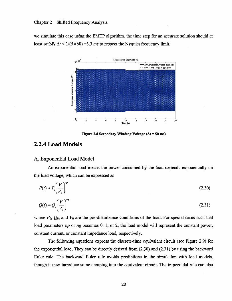
As a test case, a two winding transformer with the on-load tap changer (OLTC) is
simulated using the SFA model. The rated line-to-line voltage of the primary winding is 110kV.
The winding ratio is N1: N2 = 110 : 28.4. R = 10 , X 33.2174 2. The transformer is first
connected to the rated voltages and operating until the primary winding voltage suddenly drops
to 0.95 p.u. at t = lOs. Five seconds later, the secondary side OLTC changes the tap ratios to 1+
0.0125, attempting to bring the voltage back. The total simulation time is 20s. Figure 2.8
illustrates the dynamic phasor result together with the time domain result transformed back from
SFA solution. In this simulation, a very large time step At = 50 ms is used. On the other hand, if
19
Chapter 2 Shifted Frequency Analysis
we simulate this case using the EMTP algorithm, the time step for an accurate solution should at
least satisfr At < 11(5 x 60) =3.3 ms to respect the Nyquist frequency limit.
Figure 2.8 Secondary Winding Voltage (At = 50 ms)
2.2.4 Load Models
A. Exponential Load Model
An exponential load means the power consumed by the load depends exponentially on
the load voltage, which can be expressed as
( \flp
PQ)= PoLJ (2.30)
0
( \,nq
QQ) = (2.31)0
where Po, Qo, and Vo are the pre-disturbance conditions of the load. For special cases such that
load parameters np or nq becomes 0, 1, or 2, the load model will represent the constant power,
constant current, or constant impedance load, respectively.
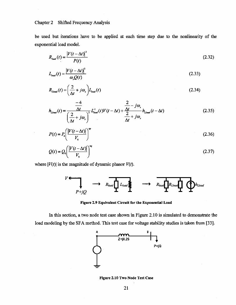
The following equations express the discrete-time equivalent circuit (see Figure 2.9) for
the exponential load. They can be directly derived from (2.30) and (2.31) by using the backward
Euler rule. The backward Euler rule avoids predictions in the simulation with load models,
though it may introduce some damping into the equivalent circuit. The trapezoidal rule can also
Transformer Test Case 02
— SFA Dynamic Phasor Solution
zsrV_ - V
0 2 4 6 8 10 12 14. 16 18 20Time (s)
20
Chapter 2 Shifted Frequency Analysis
IV(t - At)12RlOOd (t) =
P(t)
V(t - At)12kOd(t) =
oQ(t)
RL1d(t) = + JO)0 L10 (t)
—4 2
hLld(t)= At L1 (t)V(t — At) + At —
2 hL,d (t — At)(2
At
load
I + JoiAt
P(t)Iv(t—At)
=
(VQ—At)jiq
vc
P+jQ
—b Roa’ Lload —, RlaRLl0 hLload
Figure 2.9 Equivalent Circuit for the Exponential Load
In this section, a two node test case shown in Figure 2.10 is simulated to demonstrate the
load modeling by the SFA method. This test case for voltage stability studies is taken from [33].
Figure 2.10 Two Node Test Case
be used but iterations have to be applied at each time step due to the nonlinearity of the
exponential load model.
(2.33)
(2.34)
(2.32)
(2.35)
(2.36)
(2.37)
where I V(t)I is the magnitude of dynamic phasor V(t).
A B
ZjO.25
P+jQ
21

Chapter 2 Shifted Frequency Analysis
First, the system is operating with the load P= O.8p.u., and Q=O.4p.u. The load voltage at
node B is illustrated in Figure 2.11. It can be seen that the SFA curve is the complex envelope of
the time domain curve, to which the SFA result can be accurately transformed.
Two Node Test Csse Two Node Test Case
92
90
88>
86
84
-—0 1 2 3 4t (a)
(a) (b)
Figure 2.11 Simulation Results of the Node Voltage (a) SFA Solution (At = 10 ms) (b) EMTP Solution (At =
0.5 ms)
Second, the system is operating with a heavier load of P= 1 .85p.u., Q=O.1 5p.u. From the
nodal voltage shown in Figure 2.12, it can be seen that the system collapses in this case. These
results in Figure 2.12 are almost the same as the results obtained in [33], where the system is
found to collapse when P=1.843p.u and Q=O.15p.u.
Two Node Test Case
Figure 2.12 Simulation Results of Voltage Collapse (a) SFA Solution (At 10 ms) (b) EMTP Solution (At = 0.5
Now the system performance is simulated when the system load keeps increasing with
time. The system load is assumed to change in the way shown in Table 2.1. The SFA results of
22
- 0 0.2 0.4 0.6t (s)
0.8
Two Node Test Case
t (s)
ms)
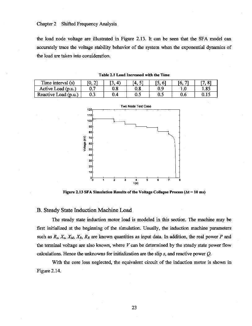
Chapter 2 Shifted Frequency Analysis
the load node voltage are illustrated in Figure 2.13. It can be seen that the SFA model can
accurately trace the voltage stability behavior of the system when the exponential dynamics of
the load are taken into consideration.
Table 2.1 Load Increased with the Time
Time interval (s) [0, 2] [3, 4) [4, 5] [5, 6] [6, 7] [7, 8]ActiveLoad(p.u.) 0.7 0.8 0.8. 0.9 1.0 1.85
Reactive Load (p.u.) 0.3 0.4 0.5 0.5 0.6 0.15
Two Node Test Case12C
110
100
______
901
80
70
, 60
50
40
t (s)
Figure 2.13 SFA Simulation Results of the Voltage Collapse Process (At = 10 ms)
B. Steady State Induction Machine Load
The steady state induction motor load is modeled in this section. The machine may be
first initialized at the beginning of the simulation. Usually, the induction machine parameters
such as R, X, XM, XR, RR are known quantities as input data. In addition, the real power P and
the terminal voltage are also known, where V can be determined by the steady state power flow
calculations. Hence the unknowns for initialization are the slip s, and reactive power Q.
With the core loss neglected, the equivalent circuit of the induction motor is shown in
Figure 2.14.
23

Chapter 2 Shifted Frequency Analysis
P + jQ,
X--
XM :RIs
Figure 2.14 Steady State Equivalent Circuit
The formula to calculate the initial slip s and the reactive power Q can be derived [34]
based on the equivalent circuit in Figure 2.14, as expressed below.
RR (2.38)_g2 -4AC
Q=Im(V2Y) (2.39)
where
A=A’---RV2
B=B’---X C=C’---RS(XS+XM)V2
A’ = + (x + XM)2 B’ = 2RX C’ = (XSXM + XSXR + XRXM
)2+ R:(xR + XM)2
Then the initial slip can be validated by checking whether the power factor falls into a
reasonable range, for instance,
0.7<cosq=cos arctan2 <0.9P-I
If the inequality is not satisfied, an error message will be printed.
The discrete time equivalent circuit in the shifted frequency domain is shown in Figure
2.15. The phasor dynamics are introduced to the steady-state equivalent circuit to capture the
dynamics in the electrical part. The parameters in the SFA model can be obtained as follows.
1G23=
2LR + + KLS
s=2A
3
Figure 2.15 Discrete Time Equivalent Circuit
(2.40)
24

Chapter 2 Shifted Frequency Analysis
1G
2L(2.41)
+
1G30 = (2.42)
R
sQ — At) At
4L 2L—R +—-—KLS
hjj_ (t) = —[v (t — At) — v (t — At)] At S At2 + 2L
hstator (t — At) (2.43)
R +_!+KLS
— KLAt Athm (t) = J/ (t — At)
+ K2
+ 2Lmhm (t — At) (2.44)
At Lm)—+KLfl
- Rr
At s(t — At) At+ h1 (t — At) (2.45)
Rr +---+K2 R 2L
h, (t) = —J (t — At)
st — At) At sQ — At) AtLrJr
When the system voltages change, there is a mismatch between the electromagnetic
torque and mechanical torque since mechanical torque usually cannot change instantaneously.
Then the acceleration equation of the rotor mass is represented as
ITm (2.46)dt pdt
where pf is the number of poles.
Therefore the slip can be calculated using the backward Euler rule,
sQ) = sQ — At) — PjII (t)
— Tm (t)]At (2.47)200J
where
V (t)
(2.48)I(t)32 Er Rr
[Rm+ s(t — At)
+ (XTH + Xr)2]
If the mechanical torque is assumed to be a quadratic function of co,
25
Chapter 2 Shifted Frequency Analysis
(2.49)=a +13s(t—/xt)+ys2(t—eXt)
where
at=a+bas+ccos2 y=ccos2
v -v XR -
—
+ (X + XM)2 m
— R + (X + X, )2
x — RX1 + xsX (X + X)TH R2+(X+X)2
Equation (2.49) represents constant torque if a = 0 and b = 0, and a torque linearly
dependent on o. if c = 0.
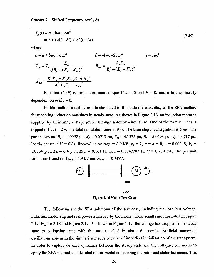
In this section, a test system is simulated to illustrate the capability of the SFA method
for modeling induction machines in steady state. As shown in Figure 2.16, an induction motor is
supplied by an infinite voltage source through a double-circuit line. One of the parallel lines is
tripped off at t = 2 s. The total simulation time is 10 s. The time step for integration is 5 ms. The
parameters are R3 = 0.0092 pu, X. = 0.0717 pu, X, 4.1375 pu, Rr = .00698 pu, Xr .0717 Pu,
inertia constant H = 0.6s, line-to-line voltage 6.9 kV, pj = 2, a = b = 0, c = 0.00308, V0 =
1.0064 p.u., P0 0.4 p.U., Rime = 0.161 2, Lime = 0.0042707 H, C = 0.209 mF. The per unit
values are based on Vbe = 6.9 kV and Sbase = 10 MVA.
The following are the SFA solutions of the test case, including the load bus voltage,
induction motor slip and real power absorbed by the motor. These results are illustrated in Figure
2.17, Figure 2.18 and Figure 2.19. As shown in Figure 2.17, the voltage has dropped from steady
state to collapsing state with the motor stalled in about 6 seconds. Artificial numerical
oscillations appear in the simulation results because of imperfect initialization of the test system.
In order to capture detailed dynamics between the steady state and the collapse, one needs to
apply the SFA method to a detailed motor model considering the rotor and stator transients. This
Figure 2.16 Motor Test Case
26

600(
500(
400(
— 3001
1 2 3 4 5 6 7 8 9 10Timo (s)
2.3 Numerical Accuracy Analysis
As mentioned in Chapter 1, the theory of Shifted Frequency Analysis (SFA) needs to be
implemented in a circuit analysis program such as the EMTP to achieve its advantage of using
large solution step and getting correct simulation results in the neighborhood of the 60 Hz
frequency. In the EMTP, a numerical discretization rule (integration rule) is used to convert the
27
Chapter 2 Shifted Frequency Analysis
is further investigated in Chapter 4, where a general-purpose induction machine model in the
shifted frequency domain is proposed.
8000
7000
2000
I000
Figure 2.17 Induction Motor Terminal Voltage (At =5 ms)
-x 10’
2 3 4 5 6 7 8 9T,mo 6)
Figure 2.18 Real Power Absorbed by the Induction Motor (At = 5 ms)
2 3 4 5T.oo 6)
Figure 2.19 Slip of Induction Motor (At = 5 ms)

Chapter 2 Shifted Frequency Analysis
equivalent circuit of each network component into an equivalent discrete time model consisting
of an equivalent resistance and a history term. These equivalent circuits of components are used
to build the nodal equations of the whole system, which can be solved by using the numerical
linear algebra. The trapezoidal and backward Euler rules are the most common choices to
perform the discretization from continuous time models into discrete time models.
An illustrative and effective way to analyze the numerical accuracy of an integrator
(integration rule) is to examine the behavior of an inductance L with v(t) as input and 1(t) as
output (or a capacitance C with 1(t) as input and v(t) as output) [30]. The magnitude and phase
distortion introduced by an integrator can be quantitatively analyzed by calculating the frequency
domain equivalent circuit of L which is discretized by the given integration rule. This approach is
adopted in this section to analyze the numerical accuracy of an integrator in the SFA domain.
To analyze frequency responses of an inductance L, first take an input that has only one
frequency co (close to w) and a unity magnitude, i.e. v(t) = cos cot.
The dynamic phasor of v(t) in the SFA domain is
V(t) = [v(t) + jH(v(t))]e’ = ej°°’ = e°’ (2.50)
Now suppose the output is
1(t) = Y(Aco)e’. (2.51)
where ) (iXco) is the admittance of an L in the discrete-time SFA domain.
A. Frequency Domain Equivalent Circuits for L
The SFA domain equivalent circuit of L is obtained with the trapezoidal and backward
Euler rule. The equivalent circuit parameters can be plotted as functions of Af (=.4), as is2r
shown in Figure 2.20.
Substitute (2.50), (2.51) into the difference equation it is easy to find Y(z\co) for each
discretization rule.
(1) Trapezoidal rule
With trapezoidal rule,
V(t)= (._+foJ3LJI(t)_ VQ—At) + —._!+JcoLJI(t—At) (2.52)
Substitute (2.50), (2.51) into (2.52),
28
Chapter 2 Shifted Frequency Analysis
e30f +et
=+ foLJYe3c0t + + jwLej&0(t
Then
— 1 — 1—
2L e°t —1 — /Xa/XtjcoL+—• tan
S 2t e + joL+jAoL•AoizV
2
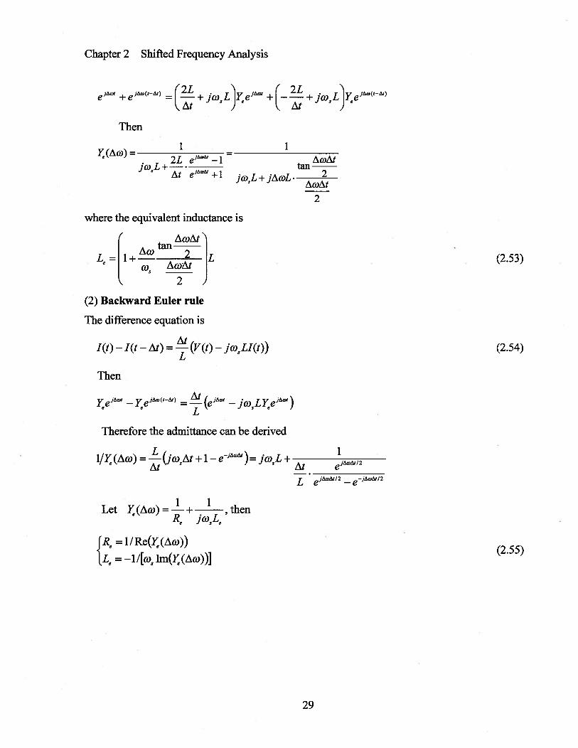
where the equivalent inductance is
AoiAttan
Le= 2 L (2.53)AoAt
2
(2) Backward Euler rule
The difference equation is
1(t) — I(t — At) = .4 (v(t)—jo5LIQ)) (2.54)
Then
— Ye W(t&) =— josLYee’)
Therefore the admittance can be derived
l/}(Aco) = ——(joi5At+ 1— e)= jo5L +A
L e’°”2 — e°’2
Let Y (Ao) =+ 1
, thenRe J(Ds1e
IR = 1 / Re(Y (Am))e e (2.55)= —ii[o Im(1’(Ao))J
29

Chapter 2 Shifted Frequency Analysis
B. Accuracy of Discretization Rules
The accuracy of the discrete-time integration rules can be expressed by the following ratio
H(Aw) = (Aa)(2.56)
H(Aco) Y(Aco)L=1
(1) Trapezoidal rule
He(CO)— Js
HQo) —2 —1
JcO+—•S At ej0( + 1
-10)5
— 2 ej2’1
At + 1
(2) Backward Euler
H(o)—
_____________
H(a) — jco5At +1 — e3A0S
= j0)5At
jo5At + 1 —
-1 0z f(Hz)
Figure 2.20 Equivalent Circuit Le for Backward Euler and Forward Euler (L=1; t =1 cycle, 3 cycles, 5 cycles)
30
(b)
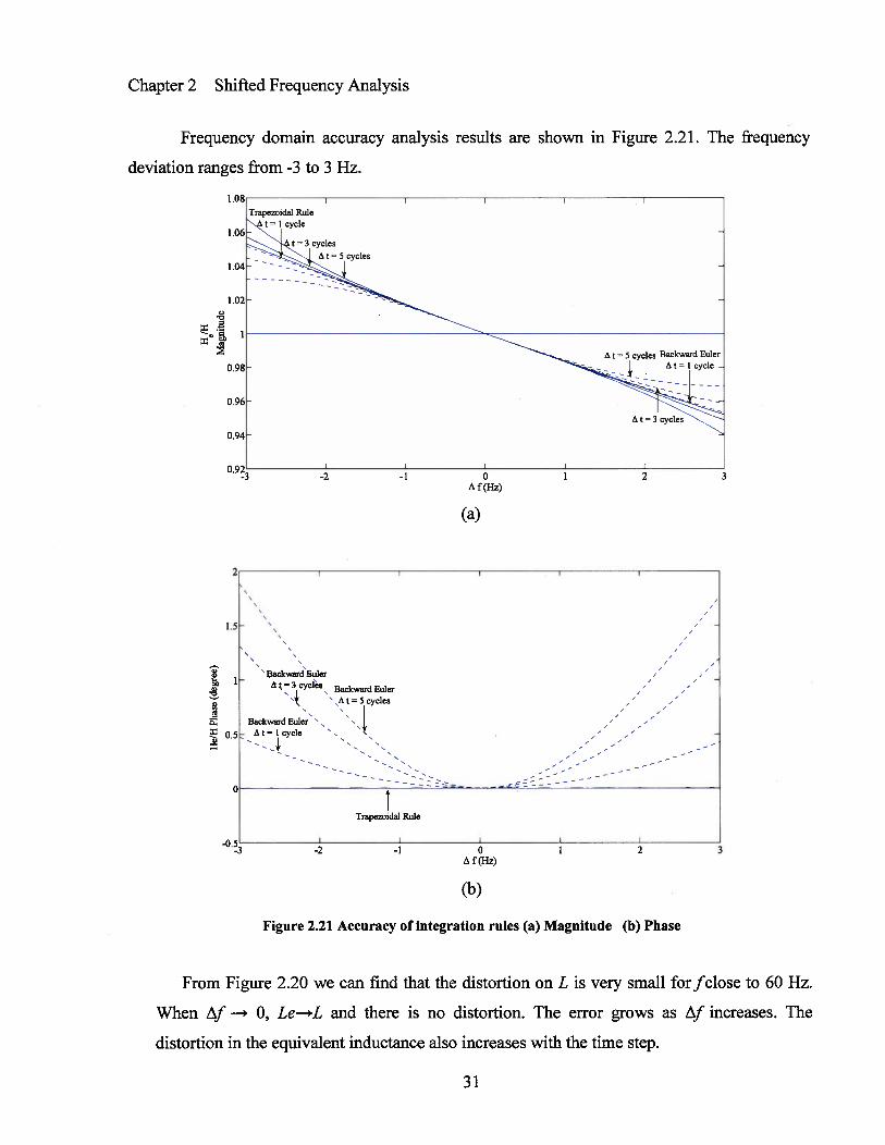
Figure 2.21 Accuracy of integration rules (a) Magnitude (b) Phase
From Figure 2.20 we can find that the distortion on L is very small for fclose to 60 Hz.
When Af —* 0, Le—*L and there is no distortion. The error grows as txf increases. The
distortion in the equivalent inductance also increases with the time step.
Chapter 2 Shifted Frequency Analysis
Frequency domain accuracy analysis results are shown in Figure 2.21. The frequency
deviation ranges from -3 to 3 Hz.
0
A f(H.z)
(a)
I I I — I I
1.5
0
Cs
0.5
ackward EulerA = 3 cycles. Backward Euler
‘5At5 cycles
Backward Euler.Atlcycle
tTrapezoidal Rule
-2 —l 0A f(Hz)
31

Chapter 2 Shifted Frequency Analysis
Figure 2.2 1(a) shows that the trapezoidal rule is slightly less accurate than the backward
Euler rule in the shifted frequency domain. On the other hand, Figure 2.2 1(b) shows that the
trapezoidal rule has no phase distortion while the backward Euler rule can cause larger phase
distortions especially when Afbecomes larger.
It is clearly shown in equation (2.55) that the backward Euler rule adds a fictitious
resistance to the circuit, which introduces numerical damping. Therefore, it may be
advantageous when the trapezoidal rule has the risk of numerical oscillations when it is used
as a differentiator. Here the backward Euler rule may be used over a few integration steps to
damp numerical oscillations whenever some discontinuities occur, which is the major idea of
CDA [30].
Unless specially noted, in this thesis the trapezoidal rule is used for the component
modelling and the system solver because SFA equivalent circuits similar to those in the
EMTP can facilitate the implementation of SFA concepts in the EMTP algorithm.
32

Chapter 3 Synchronous Machine Modelling Based on Shifted Frequency Analysis
Chapter 3
Synchronous Machine Modelling Based on
Shifted Frequency Analysis
3.1 Introduction
This chapter describes a new synchronous machine model based on the Shifted
Frequency Analysis (SFA) method, which uses dynamic phasor variables rather than
instantaneous time domain variables. Discrete-time SFA component models have a form which
is similar to the EMTP component models. Dynamic phasors provide envelopes of the time
domain waveforms and can be accurately transformed back to instantaneous time values. When
the frequency spectra of the signals are close .to the fundamental power frequency, the SFA
model allows the use of large time steps without sacrificing accuracy. This makes the SFA
method particularly efficient for power system dynamics.
3.2 Voltage-behind-Reactance Synchronous Machine
Model
The SFA method can be applied to a number of synchronous machine models, such as
the phase domain synchronous machine model of [35], the voltage-behind-reactance (VBR)
model of [36], and others. As reported in [37], the VBR model is more efficient and stable than
other traditional machine models used in the EMTP and it was chosen for the SFA
implementation in this chapter.
33

Chapter 3 Synchronous Machine Modelling Based on Shifted Frequency Analysis
Cs,
bs axis as
bs
Figure 3.1 Salient-Pole Synchronous Machine and Its Windings
The cross-section of a salient pole synchronous generator is shown in Figure 3.1. The
generator has a 3-phase stator winding, a rotor field winding (fd winding), M rotor damper
windings in the q-axis (kql, ..., kqM), and N rotor damper windings in the d-axis (kdl, ..., kdN).
The equivalent circuit in Figure 3.1 can be used for modelling different types of synchronous
machines without losing generality since straightforward changes can be made without much
difficulty to adapt this model for other types of synchronous machines. In this chapter, some
assumptions [38] are made in developing the mathematical model of the synchronous machine:
The 3-phase stator winding is assumed to be symmetrical;
The capacitances of all the windings are neglected;
Each of the distributed winding can be represented by a concentrated winding;
34

Chapter 3 Synchronous Machine Modelling Based on Shifted Frequency Analysis
The change in the inductance of the stator windings due to rotor position is sinusoidal and
does not contain higher harmonics;
Hysteresis loss is negligible while the effect of eddy current is included in the damper
winding models.
In Figure 3.1, the motor convention is adopted for the machine modelling, which means
the stator currents are positive when flowing into the machine terminals. The damper windings
are shown to represent the. paths for induced rotor currents. In a salient-pole machine, the rotor is
laminated and therefore the damper winding currents are largely confined to the cage windings
embedded in the rotor surface. Usually the dynamic behaviour of the salient-pole machine can be
predicted accurately enough by using one equivalent damper winding kq2 in the q-axis and one
damper winding kd in the d-axis. On the other hand, a cylindrical-rotor machine has a solid iron
rotor with a cage-type winding embedded in the rotor surface, and the damper winding currents
can flow either in the cage winding or in the solid iron. In order to accurately simulate the
transient process in the cylindrical-rotor machine, it is necessary to put two equivalent damper
windings kql, kq2 in the q-axis and one damper winding lcd in the d-axis.
The dqO synchronous machine model is most widely used in power system
electromagnetic transient simulations. However, to interface the dqO model to the network in the
phases a, b, c coordinates, some electrical variables have to be predicted, which may
theoretically cause numerical instability. The dqO model needs prediction because the dqO
electrical variables are not solved simultaneously with abc external network variables. A phase-
domain model avoids predicting the electrical quantities and therefore is more robust than the
dqO model. The SFA model implemented in this Chapter is based on phase coordinates and
therefore does not need predictions of the electrical variables. A detailed discussion of the
prediction in EMTP machine models can be found in Chapter 8 of [9].
The original phase-coordinate synchronbus machine model consists of three stator
voltage equations, M + N +1 rotor voltage equations, M + N +4 flux linkage equations, and
mechanical part equations for the torque and speed. To improve the numerical efficiency and
stability, a new phase-coordinate model called Voltage-behind-Reactance (VBR) model has been
derived in [36]. The rotor voltage equations and flux linkages equations are manipulated so that
the derivatives of the rotor flux linkages are algebraically incorporated into the stator voltage
equations, resulting in an efficient voltage-behind-reactance form model. The VBR model for the
35

Chapter 3 Synchronous Machine Modelling Based on Shifted Frequency Analysis
synchronous machine in Figure 3.1 includes the stator voltage equations, flux linkages equations
and rotor mechanical part equations, which can be stated as follows.
A. Stator Voltage Equations
va (t) = r5iabcs (t) + P[Lbcs (0r )‘abcs (t)] + (t) (3.1)
where r5 is the stator winding resistance matrix, and
L:bcs(Or)=L+(—L:)A (3.2)
L,+L: - -
L” = — —s- L + L” —0 2 Is2
• —--s- —--s- L15+L’
cos(20r) C0S(28 — 2?r/3) Co5(20 + 2n/3)
A = C05(20 — 2n/3) C05(20r — 47r/3) cos(20r)
cos(20r + 2nj3) cos(20r) cos(20r + 42r/3)
L”= LZq + Ld
a 3
L0”= — L’
M-1
L:q =1/Lmq +1/LlkJ ‘
N-1
Ld =1/Lmd +1/L1+1/L ,
(As an example, for a salient-pole machine, L,0 and L,d may be expressed as
Lq = (1/Lmq + 1/L,2)‘ , L = (1/Lmd + 1/L1 + 1/Lw )‘. Otherwise, L,q = (1/L,,3q+ 1/L,1 + 1/LIkq2)’
Ld = (1/Lfl,d + 1/Llka + 1/Lw )‘ may be used in modelling a cylindrical-rotor machine.)
The subtransient voltages in equation (3.1) can be expanded
V:bcs(t) = [K’(O(t))J_1 v (3.3)
0
36

Chapter 3 Synchronous Machine Modelling Based on Shifted Frequency Analysis
where
Vq = OrLmN ,2 “ M Lmqr
(LM L2mqr,qj •r (3.4)fd +
+
_____
kqi
_____
L j1 L1) j=1 L2,kmq
— k) +L2,k
1qi j=1 lkaj
M) N”
+—L mdl ds
f= lkqi 1=1 L,k L21LmdL+_2]
r .2Vd Lrnq+
Lmar,jj
[T,.
(AfdN A.
(3.5)
+‘‘fd E, N
J +rfd 2
null —+---— — L r
L2L L L L”fd 1=’ Ikdj
B. Flux Linkages Equations
—-s- ctP’kqi= L . kqj — kq) ,f = 1, 2, ..., M (3.6)
Ikqj
r(3.7)
Ikdj
—‘A. A.md)+Vfd (3.8)Pfd L fd
fd
where
MA.
= Lmq (-- + qs) (3.9)J1 lkqj
A. NA.
Ad =Lmd(++ldS) (3.10)L j=1 L,
C. Mechanical Part Equations
P8r0JJr (3.11)
PWr°jTm) (3.12)
f(2isqs Aqslds) (3.13)
where
M
Aqs L’qlqs (3.14)
37

Chapter 3 Synchronous Machine Modelling Based on Shifted Frequency Analysis
(A NA
(3.15)Lifd =1L1)
Discretizing the above VBR model with the trapezoidal integration results in a more
flexible and robust EMTP-type model than the qd0 model [37]. The qdo model is numerically
efficient and is widely used in EMTP simulators. However, the interfacing of qd0 quantities with
the electrical network, which is modeled in abc coordinates with the EMTP, is not direct and
requires some prediction. The SFA model proposed in this chapter is based on the VBR model.
Therefore, the SFA model is still in abc coordinates and the interfacing in the EMTP or in a
hybrid environment like the OVNI [39] simulator does not require prediction but interpolation
(in a similar way to what is discussed in reference [40] for the coupling of different size time
steps). Section 3.3 details the development of the SFA-based synchronous machine model.
3.3 Synchronous Machine Modelling with SFA
3.3.1 Synchronous Machine Model Based on SFA
The following equations are based on the salient-pole generator with one field windingfd,
one damper winding kd in the d-axis, and one kq2 damper winding in the q-axis. These formulas
can be modified with minor efforts for synchronous machines with arbitrary numbers of
windings in the d- and q-axis, following the procedures in Section 2.1.1.
To construct the SFA-based stator voltage equations, we first rewrite the electrical
variables using equation (2.5)
‘abcs (t) = acsi (t) cos cost — ‘ abcsQ (t) sin co5t (3.16)
Vabcs (t) = VabCSI (t) cos oit— VabcsQ (t) sinco5t (3.17)
Substituting equation (3.16) and equation (3.17) into equation (3.1) results in
VabcsI (t) cos °‘! — V abcsQ (t) sin cost
= r5 L’abcsJ (t) cos ot— abcsO (t) sin (,itj + L [P1abcsl (t) cos (flat
— ‘abcsl (t)0)5 sin o1)st
— P1 abcsQ (t) sin ot— acs (t)o5 cos5tj — L,’ {p[A cos ot] ‘ abcsl (t) + A cos oi3t . P abcsl (t)
— P[45h1 oJ5t]abcsO (t) — Asina3t PabcsQ (t)}+VbCSJ (t) cost— VbCSO (t) sin ot (3.18)
38

Chapter 3 Synchronous Machine Modelling Based on Shifted Frequency Analysis
Applying the Hilbert Transform to the left hand side (LHS) and right hand side (RHS) of
(3.18), respectively, we can construct the analytic signal (3.19), as follows
VabcS (t)et = r5 ‘abcs(t)e°’s’ +Lg [Plabcsl (t) + füI abcsl
(t)Je.b0)t
—4 {j(2ü + )Kalabcs (t) + J(2Or — UJs )K bI abcs (t)
+ KaPIabcs (t) + K bP’ abcs (t)} + Vabcs (t)e°t (3.19)
Here ‘abcs (t) , Vabcs (t) are the dynamic phasors of stator currents and voltages,
respectively; I atcs (t) is the conjugate ofI abcs (t) . K a and Kb are expressed as
ej(28. +or)
ej(28. +t—2ir/3)
ej(28 +t+2,/3)
Ka = ei(20_23) ej(280st_42r3) e1(280t)
ej(2O +t+2r/3)
ej(28, +t)
ej(28 +t+4,r/3)
ej(29 —t)
ej(28,. —at—2r/3)
Kb = ej(28r —t—2i/3)
ej(29 —t—4ir/3)
ej(28 —at)
ej(20. —,t+2nj3) e1(28, —ot)
Performing the frequency shifting as explained in equation (2.7), the SFA based formulas
for the stator voltage equations can be expressed as
Vabcs (t) = r5 ‘abcs (t) +L [PIabcs (t) + Jo sI abcs (t)j+
+ J(2COr + co5 )L e ‘abcs (t) + J(2COr — 0)s )L “ej(2o,—2f)1
abcs (t)
+ L”e2p1 abcs (t) + LeJ(28_2o)1)pI *
abcs (t) + V:bcs (t) (3.20)
where
1
L=—-- a2 a=ef2V13.
a
The SFA formulas for the subtransient voltages Vbcs (t) can be derived using the same
approach described above.
3.3.2 Discrete Time Model
Discretizing (3.20) with the trapezoidal rule of integration and rearranging,
39

Chapter 3 Synchronous Machine Modelling Based on Shifted Frequency Analysis
Vabcs(t) = A1 Iabcs(t)+A21*abcsQ)+A3I ai,cs(t — At)+A41*abcsQ
— At) + V:bCS(t)
+Vabcs(tAt) —VObCS(t—At) (3.21)
where
A1=r +I—+fJL +_+jwLneJ29
A2 =I_+jcAt
JLe1(29t)_2øo)
A3=r +I——+4 2
“L” +‘___+joLffe12t
At0J ° At
A4 =1 ——+ja JLej(20__2t_
Equation (3.21) can be further decomposed into real and imaginary parts
rvabcsr (t)1 EA1r + A2r — A1, + A2,][Iabcsr (t)
[Vacsi (t)j = [A1, + A2, Air — A21 ‘abcs,i
rVn (t)1 rA31 +A4r —A3,+A4jTIabcsr(tAt)lI abcs,r
[v:bcS,(t)j LA3,, +A4, A31 —A41 ][Iabcs,,Q_At)]
r’Vlf (t—At)1 EVabcsr(tAt)I abcs,r
+ V” (t — At)]— L VObCSZ (t —At)]
(3.22)L abcs,,
The discrete time formulas for the subtransient voltage can be similarly derived, giving
V” (t) = K(t)Ib(t)+e(t) (3.23)abcs
The time-varying factors K(t) and e (t) are expanded as follows
r e°’ ef(o_a_,r/2) ii
e (t) = e°243 ei(O_mst_23_2) 1j(8 —o,t+2/3) —,t+2,/3—/2) ij
t—At)1 1[KI2(t — At) +K2[
— At)]+ K3vf (t) + K4v(t — At)
+ [K (° (t))]
0 ]2 Fcos(Q (t — At)) cos(O,. (t — At) — 22r/3) cos(01(t — At) + 2n/3)l
Lsrn(Or (t — At)) sin(Or (t — At) — 2r/3) sin(Or (t — At) + 22r/3)](t — At)K6]—
0
(3.24)
40

Chapter 3 Synchronous Machine Modelling Based on Shifted Frequency Analysis
_1rK9 K10 0K(t)=[K’(O(t))]
[ 00][K(Or(t))] (3.25)
where
Ecos(Or) COS(Or — 2ir/3) COS(Or + 2r/3)l21
K;(or) = __[Sin(Or) Sjfl(Or — 2r/3) Sjfl(Or + 2r/3)1 1 1 I2 2 2 i
is the Park’s transformation matrix, and
L”r 1L”
_______
mq Imq kq2 ...f!.L_1] 2—At---’1—L”
L2
________________
_CUr(t)Ll2A1jlLN
lkq2 Llkq2 Llkq2 L,2J
nq I
Llkq2 ] Llkq2 Llkq2J
r
LJ LLK2 =K7 •K8 IL” N
L1 L Llkd [ L1 )J[At-- Lrnd
2- At1 1-
01K3 K4
ml
[LJ
= +_I
r\1K4 =K7 •K8
LiL:qrkq2
“ L”
L2
_____
r(J2Ltq
)r(t)l2+Athl_L
NK lkq2 l\Ikq2
L,,,2
mq
Llkq2 J Llkq2 Llkq2J
At“
fdnd
Ifd IK6=K7•K8•
At’_“kdmd I
Lj
L” L”(Or(t)
LK7JLr Ldrffl(L” Lr L”r
_________ ________ _________
,,,d kd I rnd
__ __
d_1
L2L + L2[
md
_______ ________ _______
LL + L lfd lkd lkd llf
41

Chapter 3 Synchronous Machine Modelling Based on Shifted Frequency Analysis
K9=K +
0
K10=K6+
!kd
Equation (3.23) is then decomposed into real and imaginary parts
EV:bcs,r (t)1 — rKr — K1 1EI1,r (t)1 + re,r (t)
[v:bCS, (t)]— LK1 Kr JL1abcs,i (t)J Le,1 (t)
Substituting equation (3.24) into equation (3.22) produces
E”abCs. (t)1 = R E’a,0 (t)1 +ECh.r(t)
LVabcs.j (t)]eq
[Iab, (t)] [eh, (t)
where
EA1r +A2r +K —A1, +A21 1Req =[ A11 +A21 A1 A2r+K]
reh,r (t)1 = EA3,r + A4 — A31 + A4 (t— At)1 + rVabcS. (t
— At)1 — rva,r(t
— At)1 +
[ehl (t)] [A31 + A41 A3 — A4r ][Iasi (t — At)] LVa”bCS,I (t — At)] [Vabcsi (t — At)]
EC,r (t)
[e1Q)
Equation (3.27) is the SFA-based formula, which has a similar form to the phase
coordinates EMTP synchronous machine model of [41]. The SFA equivalent circuit is shown in
Figure 3.2.
rfd
LJK8 =[ -
L1 L
-‘-1In I
fdJ I
L”1kd
LJJ
(3.26)
(3.27)
42

Chapter 3 Synchronous Machine Modelling Based on Shifted Frequency Analysis
-
-
Req(t)
zvvv)
±1+
-.
..
-
Iabc,r(t) eh,r(t)
_
s-H3-H
_
+0—H+0-H
:-
Figure 3.2 SFA Equivalent Circuit of a Synchronous Generator
In each time step, the,flux linkages can be updated as follows
r2L,q
____________________
2kq2 (t) =
_____________________
—[cos(O (t)) COS(Or (t) — 2r/3) COS(Or (t) + 22r/3)]Re[Iab (t)et]
2+At-hi_-LJL,2 1\ L!kq2
2_At1”1 L” ‘mq
_______
+ LIkq2l\ LIkq2J,;1,
2+At!1i1L”
kq2(
mq I
LJ2l. ‘!kq2JJ
—1r L” 1 [rfdLd1
- I
__
LdL Lvd
2+AJL” r L”
kd mdII At kd md
U L1)J [ LlkdJ
Sjfl(Or (t) + 22r/3)JRe[Iabcg (t)e]
r U”--
LL
2+Atr L” N
imIU L/kd)
r 1fd’ I
L L (t — At)1
2 Atr N Lkdt—AtilmdI- :{ L1Jj
r U”kq2 mq
Llkq2
r ( L”2+At—-I 1——---
Llkq2 L12
• [COS(O (t — At)) COS(O (t — At) — 22r/3) cos(Or (t — At) + 2nj3)]Re[Iab (t — At)e°’]
r L””[2+At fd 1mdI
Efd(t)I- [
U U JLkd(t
— —A-r-——kd
Llkd Ld
.[sin(O (t)) sin S(Or (t) — 2r/3)
(3.28)
f2+At--”l_LN
UJ
- At--.;LL, L
2AtLtLIl4fd Lu
AtL,kd L
43

Chapter 3 Synchronous Machine Modelling Based on Shifted Frequency Analysis
2+ At --- 1’l — — At---.- At
rLZdL Lw,) LL L
— At-—-- 2 + At--1’l _.-‘l AtmdI
L1 L Llkd L L,,) L,
• [Sjfl(Or(t — At)) sin(Or(t — At) — 2ir/3) sin(OrQ — At) + 22r/3)]Re[Iabcs(t — At)e°’]
2+ At 1— ‘rnd- At —a-- !::‘.r;
+ L
L”
L L[t1vfa(t+vfd(t_At (3.29)
-At------ 2+At---I1----L1L L1 L1
2Lqs (t) = L-[cos(Or (t)) cos(Or (t) — 2r/3) cos(O,. (t) + 22r/3)]Re[Iab (t)e3°’1+ L2Lkq2 (t)
(3.30)Ikq2
ds (t) = L [sin(O (t)) 5(0r (t) — 2r/3) sin(Or (t) + 22r/3)]Re[Iabcs (t)e’ 1+ L[fd (t) +
fd lkd
(3.31)
The differential equations of the generator’s mechanical part also have to be discretized
and can be solved together with the electrical equations. The discrete time equations of the
mechanical part are expressed
‘r (t) = ‘r (t — At) + (t) + Tm (t — At)— Te (t) + Te (t — At)] (3.32)
T (t) = _.f (t)Iqg (t) + 2qs (t)idS (t)] (3.33)
Or(t) = Or(tAt)+[COr(t)+COr(tAt)] (3.34)
r (t) = or (t — At) + At[C0r (t) + U) (t — At)
— ] (3.35)
where
p is the number of poles and
‘qdOs = K (o (t))Re[Iabcs (t)et]
Refer to [9] for more detailed multi-mass mechanical part models.
44

Chapter 3 Synchronous Machine Modelling Based on Shifted Frequency Analysis
3.3.3 Note on the Cylindrical-Rotor Machine Model
The shifted-frequency-domain equivalent circuit of a cylindrical-rotor synchronous
machine is similar to that of the salient-pole machine. As mentioned in Section 3.2, however, the
cylindrical-rotor machine has different rotor windings from the salient-pole machine. Therefore,
particular equations and factors in Sections 3.3.1 and 3.3.2 have to be re-written., which can be
expressed as follows.
ei(_0t) 1
e (t) — e°’243 eJ(G 22n/3_2n/2) 1
e j(r —sr÷2/3)e
j(9,. —t+2a/3—r/2)
rAk (t—At)1 A (t—At)[K1LAt — At)jAkb2 (t — At) + K2
— At)+K3vf(t) +K4vf(t — At)]
+ [iç (o (t))]-’
[K K ]Ecos(Or (t — At)) cos(Or (t — At) — 2r/3) cos(Or (t — At) + 22r/3)11(t — At)6
[sin(Or (t — At)) sm(0r (t — At) — 2n/3) sin(Or (t — At) + 2r/3)J abcs
0
(3.36)
Lqrkql 1L L:q2rkq2 L:qrkq2(L L:q2rkql
K1Lqi 1 LlkqI ,) Lq2Llkql Lq2 L ) LqlLIkq2
Ikql !kq2
2— At-!!—I!L— i”1 — At
rkqiLrnq2+ At-_I-_ — At
rkqlLrnq
L,,,1 Ljjqi ,) LlkqlLlkq2 L,1 Lijq1 ) LIkqlLIkq2
— Atrkq2Lmq
2— At--1’-- — Atrkq2Lmq
2+ At--(i_ —
L11L12 L12 L Llkq2 ) LlkqlLIkq2 L,2 Li*q2
Lrkql [!_—
+ L:q2rkq2 L,qrkq2—
+ ‘mqkq1
K = Ikql lkql Ikq2 lkql lkq2 Ikq2 lkql lkq2
L”r(t)
L11 lkq2
45

Chapter 3 Synchronous Machine Modelling Based on Shifted Frequency Analysis
rr L”
H d’]I kql mq
—Atrkq2Lrnq
Llkql Llkq2
rkql mq-
—Atrkq2Lrnq
L,1L2
L— kql inIr
r L” N
LIql[LlkqI )—Atr2L,q
Llkql L,,2
i-I
—AtrkqlLrnq [rkq1LIql
Llkql LIkq2 Llkql
2— At—-- rnqI At kq2 mqL” r L” I
L12 [UIkq2 L Liq2 ]
L”—At
rkql mq
LikqlL1,2
rkq2 mq2_At__[___lJj
K9=K5+
-.[cos(O,. (t)) cos(9r (t) — 2nj3)
L”At1
LIkql
Atrkq2Lrnq
L12
cos(Or (t) + 2n/3)}Re[Iab (t)e°’ 1+L”
—Atrkql
L,1L12
2-L112 Lijq2
L”
LIkqIL12
L”At
rkq2
LIkqlL,2
-At--I -n--iLlkql L1,
r—At kq2 mq 2
L1,1Llkq2
[cos(O,. (t — At)) cos(Or (t — At) — 22r/3) cos(Or (t — At) + 27r/3)]Re[Iabc$ (t — At)e°’] (3.37)
Aq 0’) = Lq”- [COS(r (t)) cos(O (t) — 2n/3) cos(Or (t) + 22r/3)]Re[Iabcs (t)e°’ 1+LZq[kl(t) +212(t1
(3.38)Ikql Ikq2
Thus, it can be seen that separated subroutines have to be coded for salient-pole and
cylindrical-rotor machines when implementing them in a computer program. If both the salient
pole and the cylindrical-rotor machine could use a single model with the same number of damper
windings, this would be more convenient for the code maintenance and extension.
46

Chapter 3 Synchronous Machine Modelling Based on Shifted Frequency Analysis
Before we solve the above problem, let us first examine the subtransient reactance matrix
in the stator equation (3.2), where L0= L + (— L)A. If the dynamic saliency effect, which
means L L, can be neglected from the stator equations, we get L= L —
= 0 and L8
becomes a constant matrix. This will effectively improve the numerical efficiency in simulations.
References [42j has proposed a method to neglect the dynamic saliency effect. First, the
operational impedances are calculated based on the original parameters of the machine. Second,
an artificial q-axis winding is added in the machine model such that X’ = Xd”, at the same time,
the frequency response curve of the new operational impedance accurately matches that of the
original Xq (s) over a frequency range,U’ where f. is a user-defined frequency. By fitting
the frequency response curve of the new operational impedance, a new set of machine
parameters can be obtained.
Therefore, we can always build a three damper windings model to represent both salient-
pole machine and the cylindrical-rotor machine with acceptable frequency response. Because the
dynamic saliency is eliminated, the refitted model is numerically more efficient than that with
the dynamic saliency. We then need to develop only one uniform subroutine for different types
of synchronous machines. Thus the problem is solved.
3.4 Simulation Results
Three test cases have been simulated to illustrate the efficiency and accuracy of the SFA
model. The first two cases illustrate that the SFA model is a general purpose model, which can
simulate both slow and fast dynamics. The third case shows that the SFA model is numerically
more efficient and stable than the phase-domain EMTP model. Throughout this chapter, both the
EMTP and SFA programs for simulating the single machine dynamics are implemented and
tested in the same MATLAB environment.
The synchronous machine parameters for the three cases are shown in Appendix A taken
from [43].
A. Simulation of Slow Dynamics
The first test case consists of a salient-pole hydro turbine generator connected to an
47
Chapter 3 Synchronous Machine Modelling Based on Shifted Frequency Analysis
infinite bus. It was assumed that the system is initially operating in steady state with a
mechanical torque Tm = 0 and a field voltage Vj1 .0 p.u.
At t = 1 .Os, the field voltage is stepped down to 0.8 p.u. Later, at t = 7.0 s, the field
voltage is stepped up to 1.2 p.u. Finally, at t = 15.0 s the mechanical torque is stepped up to Tm
0.85 p.u. The total simulation time is 20 s.
The simulation results with the SFA model are shown in Figure 3.3. The variables plotted
in this figure are ‘as (phase A stator current), ld (field current), Te (electromagnetic torque), or
(rotor angle), cor (rotor speed), P (real power) and Q (reactive power); all values except for 0r are
in per unit of the machine ratings. In this simulation, a large time step & = 7 ms is used. Note
that the SFA model can produce both dynamic phasor and time domain results (refer to equation
(2.7)). The uppermost subplot in Figure 3.3 shows the magnitude of dynamic phasor for phase A
stator current. The dynamic phasor solution gives the envelope of the time domain results. The
reconstructed instantaneous time domain values were identical to those obtained with the EMTP
simulation with the synchronous machine represented with our own VBR model implementation.
The EMTP and SFA programs for simulating the single machine dynamics are both developed in
MATLAB script. The total CPU time for the SFA responses on a 1 .83G Hz PC was 7.0 s.
B. Simulation of Fast Transients
The second simulation is a three phase fault for a single machine infinite bus system. The
parameters of the hydro turbine generator used for this case are also those in Appendix A. The
system is initially operating with Tm = 0.85 p.u. and Vj = 1.0 p.u. At t =1.0 s, a three-phase fault
is applied to the generator terminals. Then, at t = 1.4 s, the fault is removed with the simulation
continuing to t = 8.0 s. The simulation is then repeated with the fault cleared at t = 1.5 s.
A & of 0.Sms was used in order to capture the fast transients caused by the fault. When
the fault is cleared in 0.4 s the system remains stable. However, when the fault is removed in 0.5
s the system loses synchronism. By repeating the simulation, we found that the critical fault
clearing time to prevent instability is close to 0.462 s. The SFA-based model gave identical
results to those of the instantaneous time domain simulation. The time domain results are from
the same MATLAB program mentioned in Section A. The CPU time needed to calculate the
SFA responses for the stable case and the unstable case were 6.13 s and 6.14 s, respectively. The
simulation results of the three-phase fault case are illustrated in Figure 3.4-Figure 3.6. Zoomed
48

Chapter 3 Synchronous Machine Modelling Based on Shifted Frequency Analysis
in views of the unstable case with fault clearing time of 0.5 s are shown in Figure 3.6, which has
clearly captured the exponentially decaying of dc offsets in three-phase stator currents.
Simulation results for a single-phase-to-ground fault are presented in Figure 3.7. This
figure shows the stator currents ‘as, ‘bs and with a fault occurring at t = 1.1 s on phase A. Two
zoomed-in segments for ‘a are embedded in the top subplot to depict the relationship between
dynamic phasor and time domain results.
Case studies (a) and (b) show that the SFA model is adequate as a general purpose
machine model. It allows us to use large time steps to simulate slow transients (case (a)), while it
can also accurately capture the fast transients if an appropriate small time step is used (cases (b)).
C. Comparison between SFA and VBR Models
In order to further illustrate the advantages of the SFA solution domain and of the
proposed SFA phase-coordinates salient-pole synchronous generator model, a third case is
simulated comparing the SFA solution with a conventional EMTP solution that uses the
improved VBR phase-coordinates salient-pole synchronous generator model. In this example, a
steam turbine generator is connected to an infinite, bus that supplies rated three-phase voltages.
The system is running in no-load steady state with Tm = 0 and = 1.0 p.u. The torque Tm is
stepped up to 1.1 p.u. att=0.1 s.
The SFA model was used with different time steps At = 0.lms, At = 1 ms and At 10 ms.
The study was repeated using the VBR model with At = 0.1 ms. The VBR model was carefully
verified in [37] against the standard EMTP model and its results are assumed to be the reference
accurate time domain results. The results in Figure 3.8-Figure 3.12 show that the proposed SFA
model can accurately simulate the system dynamics with a very large time step of 10 ms. In fact,
the simulations show that if the time step is made as large as 15 ms, we still get accurate and
stable results. Table 3.1 indicates the CPU time needed for the VBR and SFA simulations. For
the same accuracy, the VBR model needed, a At = 0.1 ms and a total CPU time of 13.266 s, while
the SFA model needed a At = 10 ms and a total CPU time of 0.26 s. A zoomed in view of phase
A stator current is shown in Figure 3.9. The SFA model was in this case 50 times more efficient
than the VBR model. As reported in [37], for the same accuracy the EMTP VBR model can use
a 50 times larger time step than the conventional dqO model [41] (e.g. 0.5 ms vs 10 its) at the
expense of about 5 times the computational time per solution step. For this rotor dynamics
49

Chapter 3 Synchronous Machine Modelling Based on Shifted Frequency Analysis
example, the VBR model in the EMTP solution frame was, therefore, about 10 times more
efficient than the dq0 EMTP model, while the new proposed SFA model in the SFA solution
frame was about 500 times faster than the dqO EMTP solution. This example illustrates the very
high advantage of the SFA model for slow system dynamics. Table II also shows that SFA
simulation is computationally more intensive than EMTP simulation for the same At step. This is
due to the higher computational cost of operating with complex numbers (SFA) as compared to
real numbers (EMTP) and also to the overhead involved in transferring between shifted
frequency domain and normal time domain. These higher costs, however, are more than
compensated for by the gains achieved by using a much larger integration step At.
It is also interesting to compare the numerical stability of the SFA machine model in the
SFA frame with that of the VBR model in the EMTP standard frame. Figure 3.13 shows that if
we run an EMTP simulation with the VBR model using the time step of 10 ms that we use for
the SFA model, the VBR model results are no longer numerically stable. It is known that the
integration rule can only give reasonably correct results when the maximum frequency in the
simulation is at least five times less than the Nyquist frequency fNyquist = 1/(2fm)[30]. In other
words, the time step At should be less than 1/(5x2x60) = 1.67 ms for an EMTP simulation of
fundamental frequency dynamics. Table 3.2 shows the VBR model with a 5 ms time step has
11% numerical error, which makes the result no longer usable. When the time step used in the
simulation is too large, i.e. At = 10 ms, the simulation in the unshifted time domain will become
numerically unstable. On the other hand, as can be seen in Table 3.2, the SFA model with 10 ms
time step provides much more accurate result than the VBR model with 1 ms time step, and at
the same time is five times faster than the latter.
Table 3.1 CPU Times for 4s Simulation in Case C
VBR Model SFA Model
0.lms* 13.266s* 27.012sTimeSteps lms 1.328s 2.668s
lOms* ** 0.260s**values for same accuracy ** numerically unstable
50

Chapter 3 Synchronous Machine Modelling Based on Shifted Frequency Analysis
Li
a.
0€
a. 0.5
0,I
30
€1)20
0)€1)l0
1.00.
1 .DOC
I .0O
.1.00:
0.99€
0.:
-02
-0.6
-0.1
OZ
0.15
0,1
— 005
O .0,05
-0.1
.0.15
0 2 4 6 8 10 12 14 16 19 20
‘‘5 2 4 6 8 10 12 14 16 18 2C
Figure 3.3 Simulation Results with the SFA Model for Field Yoltage and Mechanical Torque Changes (At =7ms)
- —
— EMTP SOICCOOn- —SFASOkDOn
1 2 4 6 8 10 12 14 16 18
I I I0 2 4 6 8 10 12 14 16 18 20
H2 4 6 8 10 12 14 16 18
2 4 6 8 10 12 14 16 18 2
2 4 6 8 10 12 14 16 18
I C I C I I_
51
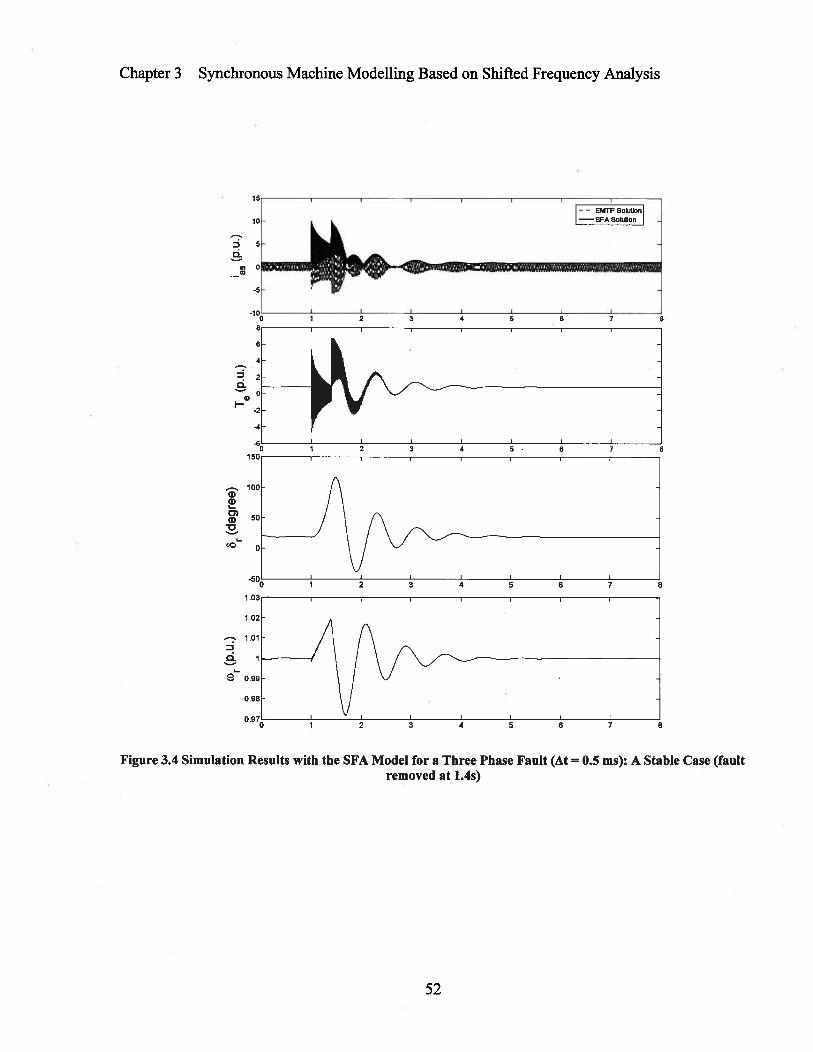
I
a)a)0)a)•0
Chapter 3 Synchronous Machine Modelling Based on Shifted Frequency Analysis
CoCU
-
- EMTP SoIutloj
150
8
Dci
2
Figure 3.4 Simulation Results with the SFA Model for a Three Phase Fault (At = 0.5 ms): A Stable Case (faultremoved at 1.4s)
52

Figure 3.5 Simulation Results with the SFA Model for a Three Phase Fault (At = 0.5 ms): An Unstable Case(fault removed at 1.5s)
Chapter 3 Synchronous Machine Modelling Based on Shifted Frequency Analysis
15 I I I
I EMTP Solution I
isFASoluuoa
ic I I I I I I
0 1 2 3 4 5 6 7
2 3 4 5 6 7
4000
a)2 30000)a)_ 2000
to1000
a.
$
t I 2 3 5 6 7
53

Chapter 3 Synchronous Machine Modelling Based on Shifted Frequency Analysis
1.02
1.01
0.
0.99
I 1.05 1.1 1.15 1.2 .25
Time (s)1.3 1.35 .4 1.45
Figure 3.6 Simulation Results with the SFA Model for a Three Phase Fault (At = 0.5 ms): Zoomed-in View ofa Portion of Results in Figure 3.5
Figure 3.7 Simulation Results with the SFA Model for a Single-Phase-to-Ground Fault (At = 0.5 ms)
0.
C
Ill
\ I,I 11111
Ij Il’?II I
—— EMTPSob9o1
I-si
Ii II1
I
l I! 1 II I,Ij
115 12
III II 0
lII I 1] 1 I,
cI.
0
54

Chapter 3 Synchronous Machine Modelling Based on Shifted Frequency Analysis
- - x 10
2
15
05
0
-05
—1
-1.5
-2
StorC,rentl(t)
Figure 3.8 Simulation Results by SFA: Phase A Stator Current
Figure 3.9 Simulation Results by SFA: Zoomed-in View of Phase A Stator Current
1.5
t
05
10P.IdCmnti0(A)
0.5 1 1.5 2fin,, (n)
2.5 3 3.5
Figure 3.10 Simulation Results by SFA: Field Current
SFAt0.1.-3.
SFAn,1o4n
—
— Aoo,r.t, Tin,. Oonn,in Ren,,It
—SFA5t0.1o-3
SFA8tle-3
05 1.5Inn, (n)
25 35
SFAI,r10.-3
55

Chapter 3 Synchronous Machine Modelling Based on Shifted Frequency Analysis
Electoomagneto Torque T0
z
0.5 1 1.5 2 2.5 3 3.51W,. (s)
Figure 3.11 Simulation Results by SFA: Electromagnetic TorqueRotor Speed e,
Wee(s)
Figure 3.12 Simulation Results by SFA: Rotor Speed
Table 3.2 Accuracy Comparison between SFA Model and VBR EMTP Model in Case C
NumericalModel Time Step CPU Time Error in Stator
CurrentVBR lms 1.328s 1.02%VBR 5ms 0.271s 11.0%SFA lOms* 0.260s 0.21%
I—a)
Co
CO
e
56

Chapter 3 Synchronous Machine Modelling Based on Shifted Frequency Analysis
4:
Figure 3.13 Time Domain Results Using the VBR Model (At = 10 ms)
3.4 Summary
This chapter has presented a very efficient synchronous machine model for the
simulation of slow system dynamics using EMTP modelling in the Shifted Frequency Analysis
framework. Instead of instantaneous time domain variables, the model uses time varying
complex variables (dynamic phasors). The SFA model results in an EMTP-type equivalent
circuit that retains the numerical properties of the EMTP solution at much larger integration
steps. The synchronous machine model implemented in this chapter for the SFA framework is
based on the VBR synchronous machine model, which is a very efficient implementation of a
phase-coordinates synchronous machine model. Working in phase coordinates provides a more
stable machine model than the traditional dqO model by avoiding predictions at the interface with
the external phase-coordinates power system network. The SFA framework reduces the size of
the equation set that describes the synchronous machine behaviour for large efficiency gains.
During system dynamics around the fundamental 60 Hz operating state of the system, a very
large time step can be used to capture time domain results without loss of accuracy. Speedups of
fifty times over traditional EMTP simulation were obtained for a case of mechanical torque step
changes. This proves the feasibility of using EMTP solutions in the Shifted Frequency Domain
for on-line assessment of large-scale power system dynamics. The SFA model is also capable of
simulating fast transients caused by topological changes in the electrical network by using
smaller time steps, but the extra overhead makes it slower than traditional EMTP for these
situations.
n,o ()
57

Chapter 4 Induction Machine Modelling Based on Shifted Frequency Analysis
Chapter 4
Induction Machine Modelling Based on
Shifted Frequency Analysis
4.1 Introduction
The intent of this chapter is to extend the SFA method to induction machine modelling.
Induction machines form a large portion of power system loads and serve as some Independent
Power Producer-owned generators. An accurate simulation of their dynamic behavior is therefore
required for voltage stability and transient stability, etc [7] [8]. The efficient and stable SFA
model for induction machines is well suited for such simulations in the SFA domain.
This chapter proposes a new efficient SFA model for induction machines, by combining
the SFA method with the phase-domain EMTP induction machine model. An equivalent-
reduction technique, which reduces the number of equations of stator, rotor, and flux linkages
into only those of stator variables without sacrificing numerical accuracy, is used in deriving the
SFA induction machine model. It allows the use of large time steps in simulating slow dynamics,
but the SFA model can also accurately simulate the fast transients in the induction machine,
which makes it a general purpose model.
Section 4.2 first proposes a new phase-domain induction machine model used in EMTP.
The philosophy inside the proposed equivalent-reduction (ER) approach will be described, and
case study results will also be discussed in this section. Section 4.3 extends the Shifted
Frequency Analysis method to the ER-based induction machine model, resulting in a very
58
Chapter 4 Induction Machine Modelling Based on Shifted Frequency Analysis
efficient, numerically stable model that is a valuable component for real-time EMTP simulations.
Section 4.4 summarizes the new contributions made in this chapter.
4.2 Equivalent-Reduction Approach to Induction Machine
Modelling in EMTP
Induction machines form a large portion of power system loads. Accurate EMTP
simulation of their transient behavior may be required for voltage stability, transient stability,
power quality analysis, and motor starting calculations, etc [8][44]. An efficient and stable
EMTP model for induction machines is therefore of importance.
Induction machine models being used in EMTP-type simulators are mainly dqO-domain
models [41], [45]-[48]. In terms of the ways they interface with EMTP, the dqO-domain models
[49] can be further classified into several groups. One group of dqO models, e.g. the universal
machine model [50], utilizes the compensation technique where the external system is modeled
as a three-phase Thevenin equivalent circuit and solved simultaneously with the machine
equations to obtain machine variables. Then the system node voltages are updated by using
linear superposition to take into consideration the machine effects. In order to use the Thevenin
equivalent and linear superposition, the external system seen from the machine terminals has to
be linear. Therefore, a distributed-parameter stub line has to be inserted to separate the machine
model from other machines or nonlinear elements, which usually requires very small integration
time steps [45][46]. The synchronous machine model in [41] can be directly converted to the
induction machine model by feeding it with modified data entries [46]. However, this model
requires predictions of flux linkages and mechanical variables. With this approach, the dqO
model is transformed to a phase quantities model, after application of the trapezoidal rule and
equations reduction to stator variables only. To keep the equivalent resistances constant and not
rotor-angle dependent, the d- and q-resistances are averaged, and a correction term is added to
compensate for this error. This correction term requires .prediction of the stator currents. All of
these predictions require a smaller time step than actually needed, to avoid numerical
instabilities. Other dqO models include the voltage-behind-subtransient-reactance (and armature
resistance) model and Norton-equivalent-based model [47], etc, which have similar
59
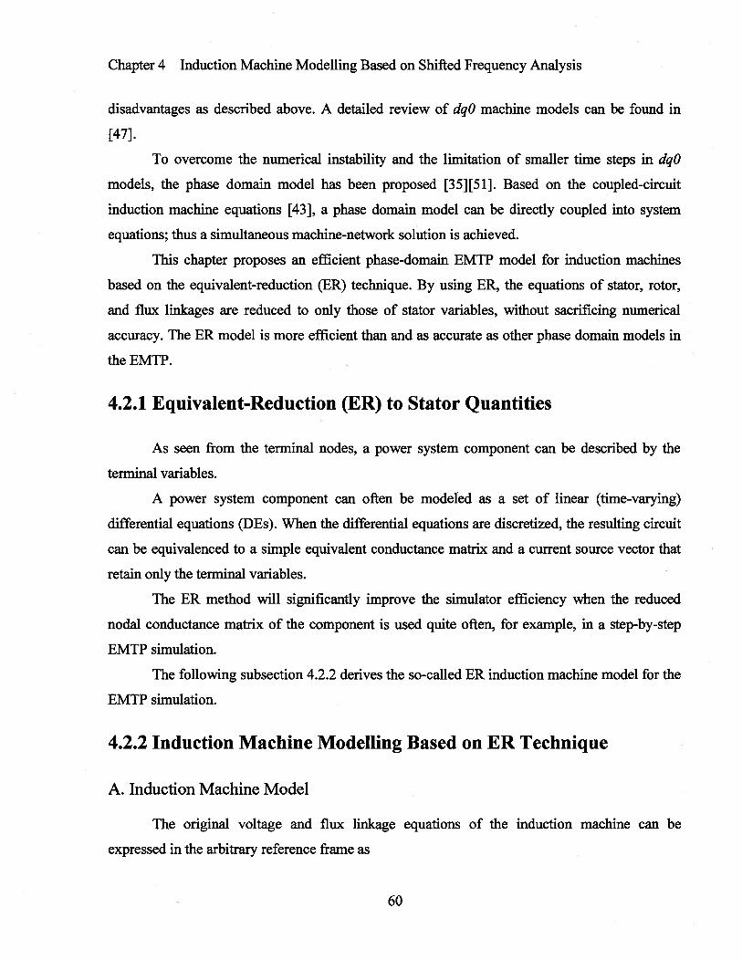
Chapter 4 Induction Machine Modelling Based on Shifted Frequency Analysis
disadvantages as described above. A detailed review of dqO machine models can be found in
[47].
To overcome the numerical instability and the limitation of smaller time steps in dqO
models, the phase domain model has been proposed [35][51]. Based on the coupled-circuit
induction machine equations [43], a phase domain model can be directly coupled into system
equations; thus a simultaneous machine-network solution is achieved.
This chapter proposes an efficient phase-domain EMTP model for induction machines
based on the equivalent-reduction (ER) technique. By using ER, the equations of stator, rotor,
and flux linkages are reduced to only those of stator variables, without sacrificing numerical
accuracy. The ER model is more efficient than and as accurate as other phase domain models in
the EMTP.
4.2.1 Equivalent-Reduction (ER) to Stator Quantities
As seen from the terminal nodes, a power system component can be described by the
terminal variables.
A power system component can often be modeled as a set of linear (time-varying)
differential equations (DEs). When the differential equations are discretized, the resulting circuit
can be equivalenced to a simple equivalent conductance matrix and a current source vector that
retain only the terminal variables.
The ER method will significantly improve the simulator efficiency when the reduced
nodal conductance matrix of the component is used quite often, for example, in a step-by-step
EMTP simulation.
The following subsection 4.2.2 derives the so-called ER induction machine model for the
EMTP simulation.
4.2.2 Induction Machine Modelling Based on ER Technique
A. Induction Machine Model
The original voltage and flux linkage equations of the induction machine can be
expressed in the arbitrary reference frame as
- 60

Chapter 4 Induction Machine Modelling Based on Shifted Frequency Analysis
Vqaos =rsiqaos +O•)Idqs +P%qdos (4.1)
0 = rriqaor + (a— “r)dqr + Pqdor (4.2)
P’s 1 = FcL:’ KLK; qaos 1 (4.3)[qaor] [KrLK:’ KrLrK;’Jiqaor]
where co is the speed of the reference frame. K and Kr are the transformation matrices that map
the stator variables and rotor variables to the reference frame [43], respectively.
B. Machine Modelling via ER
Rewriting equations (4.1)-(4.3) into a new matrix form, excluding the 0 equations
because it is already decoupled from the d and q equations, we get
FA11 A12 1qds 1 = FB11 B12 [iqds 1 + (4.4)[A21 A22][qdrJ [B21 B22 J[Iqdr•j [ 0 ]
where
L1 + LM
A11= L,S+LM
L1
LM
A12 = A21 = LM
0
L1 + LM
A22=
L1
—r3 —w(Ll$+LM) 0
B11 — + LM) —
—‘
0 —coLM
B12= coLM 0
0
0 (COCOr)LM
B21= (Ct;—cor)LM 0
0
61

Chapter 4 Induction Machine Modelling Based on Shifted Frequency Analysis
rr (OrXLlr+LM)
22 = (0—
X1tr + LM) — rr
rr
The number of equations in (4.4) can be reduced by eliminating rotor equations via ER,
as follows
= BIllqds + Bi21qar + Vqds (4.5)
where
rL’
L”
L—r —aL r
L2LIr+LM
M —rrL1 +LM
LMr -L
—L1 + LM
r r M
12 LoL M
r M L1, +LMr
L”=L,3 +LZ
L”— LILM
M T TL1 + LM
Re-arranging (4.5), including the 0 equations, and applying Park’s inverse transformation
to it, we get
Vb rsiabcs + Labcslabcs + Vres (4.6)
where
T” 1”
L+L” MIs3M
3 3
Labcs ——a- L + — —
L —-
L,5+LZ,
62

Chapter 4 Induction Machine Modelling Based on Shifted Frequency Analysis
LMr,.COTLM
L+L
= [K5 (o)]’ —
LLM rr (47)
r M L1 + LM
0
In equation (4.6), no information for rotor electrical part is lost. In fact, the rotor
information is included in Labcs and Vre5 which is an equivalent seen from the stator. Rotor
currents ‘qdr can be represented using the following differential equations derived from (4.4)
A 22’qcfr =A2iIqas +B21q + B22qdr
Discretizing the above equation for qdr, we can obtain the discrete-time equations (see
equation (4.9) in subsection C) that can be used to update qdr at each time step.
The rotor circuits have to be retained explicitly when power electronics devices are
connected to them.
C. Discrete-Time ER Model
Discretizing (4.6) with the trapezoidal rule of integration gives us
Vb (t) = + Labcs Jlabcs (t) + Vrcs (t) + ehl (t) (4.8)
where
ehl(t) = — 1dabcs )‘abcs (t — At)+ Vres(t — At)— Vb(t — At)
After applying Kron’s reduction formula [52] to the discrete-time form of equation (4.4),
we can get
qar(t) = k1 (t)Iqds (t) +k2(t) (4.9)
Substituting (4.9) into (4.7) results in
Vres = k(t)Ib (t) + eh2Q) (4.10)
The equivalent circuit of the induction machine therefore becomes
Vabos (t) = R eq’ abcs (t) + Ch (t) (4.11)
where
L1 + LM
L,1 + LM
63

Chapter 4 Induction Machine Modelling Based on Shifted Frequency Analysis
Req = r3 + L abcs+ k(t) (Equivalent resistances)
eh (t) = Chl (t) + Ch2 (t) (History term)
The factor matrices and history terms in (4.9) and (4.10) can be expanded as follows
At-A21 +B21(t)—
At[co(t)—co(t)](L, +LM)
2Air—i- + + LM
—
LM
k2(t) = A22_B22Q)4J.J [(A21+B2l(t_At)•JIqds(t_At)
+(A22+B22(t_At)4Jiqcir(t_At)]
At[a(t)— CUr (t)Lir + LM)
2Air
+ L1 + LM
—-+L1+LMAt[CO(tIXt)COr(tAt)](Lir +LM)
At[(D(tAt)COr(tAt)](Llr+LM) —-+L +L2 2 Ir M
The time-varying factors k(t) and eh2(t) in (4.10) are expressed as
AIV’A22 _B22(t)___J (
Air__: + Lir + LM
2
LM
1qds (t — At)
LM
64

Chapter 4 Induction Machine Modelling Based on Shifted Frequency Analysis
k(t) = [K(o)]_1[k3(t) 0][K5(o)]
eh2(t)= [K(e)p[jt)]
LMrrCOr(t)LM
k3(t)= I —L1 +LM
L rk1(t)
O)Q)L Mr
r M L1 +LM
LMrrO)r(t)LM
k4Q) =—
L, + LM
L rk2 (t)
O)(t)LMT
M r
lrIt should be noted that, although the equations for the rotor electrical part are eliminated,
the rotor currents could be updated at each simulation step via (4.9).
Refer to [9] and [511 for the discrete-time equations of the mechanical part.
The ER induction machine model is actually a full-order accurate phase-domain model
because the information for the rotor electrical part has already been integrated into the stator
part equations. Also, because Park’s transformation is implicitly used in the ER model, the
elegance and simplicity in the discrete-time equivalent circuit are achieved. With a lower number
of equations in the model, it is simpler and faster than traditional phase-domain models in the
EMTP, without compromise in accuracy.
4.2.3 Simulation Results
Three test cases are simulated to illustrate the efficiency and accuracy of the ER model.
The first case illustrates free acceleration characteristics of a 3-hp induction machine and a 2250-
hp induction machine. The second case is a load torque change test which shows the slow
dynamics of the 3-hp machine. The third case simulates the fast transients caused by a three
phase fault. The induction machines parameters for the three cases are shown in Table A-TI taken
from [43]. Rotor parameters have been converted to the stator side.
As reported in [37], the voltage-behind-reactance (VBR) model [36] is more efficient
than traditional phase-domain EMTP models and more stable than dqO-domain models; hence a
discrete-time VBR induction machine model used in EMTP [53] was chosen to compare with the
65
L1 + LM
Lir + LM

Chapter 4 Induction Machine Modelling Based on Shifted Frequency Analysis
ER model. To facilitate the comparison of CPU times, both machine models are deliberately
implemented in the language of MATLAB® script.
A. Simulation of Free Acceleration
The start-up transients of the 3-hp and 2250-hp induction machines during free
acceleration from stall are simulated. The total simulation times are 1 s for the 3-hp induction
machine and 3 s for the 2250-hp induction machine, respectively. In this simulation, a time step
& = 500 ,us is used.
Figure 4.1 illustrates the torque-speed characteristics of the 2250-hp induction machine
during free acceleration. The simulation results, for the 3-hp induction machine are shown in
Figure 4.2. The variables plotted in this figure are ‘as (phase A stator current), ‘m (magnetizing
flux linkage), Te (electromagnetic torque) and mechanical rotor speed. These machine variables
are observed in the rotor reference frame; results viewed in other reference frames are omitted
here.
It can be seen that the time domain values obtained from the EMTP simulation with the
ER induction machine model are practically identical to those with the VBR model. In Figure 4.1
and Figure 4.2, the results from the ER model and the VBR model are so close that they become
indistinguishable from each other. Numerical tests also indicate that both ER and VBR model,
when a large time step of 1 ms is used, can still get accurate, stable, and identical solutions.
x i04
Figure 4.1 Torque-Speed Characteristics during Free Acceleration of a 2250-hp Induction Machine (At = 500 js)
2.j’ —ER Result-
- VBR Result
I,2
0 200 400 600 800 1000 1200 1400 1600 1800Speed (rpm)
66
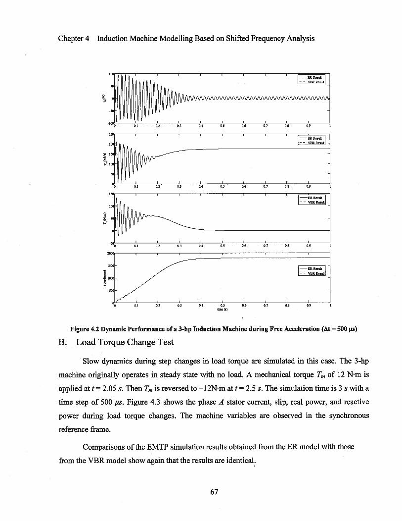
Chapter 4 Induction Machine Modelling Based on Shifted Frequency Analysis
Figure 4.2 Dynamic Performance of a 3-hp Induction Machine during Free Acceleration (At = 500 Its)
B. Load Torque Change Test
Slow dynamics during step changes in load torque are simulated in this case. The 3-hp
machine originally operates in steady state with no load. A mechanical torque Tm of 12 Nm is
applied at t = 2.05 s. Then Tm is reversed to —12Nm at t = 2.5 s. The simulation time is 3 s with a
time step of 500 ps. Figure 4.3 shows the phase A stator current, slip, real power, and reactive
power during load torque changes. The machine variables are observed in the synchronous
reference frame.
Comparisons of the EMTP simulation results obtained from the ER model with those
from the VBR model show again that the results are identical.
0.5the (s)
67

200C
1955
1905>
___________
O 1855
1805
1755
1702 2.1 2.2 2.3 2.4 2.5 2.6 2.7 2.8 2.9 3Ume (s)
Figure 4.3 Dynamic Performance of a 3-hp Induction Machine during Step Changes in Load Torque (At =
500 is)
C. Three Phase Fault Test
In this simulation of fast transients, the 2250-hp induction machine is first operating
under rated conditions with a load torque equal to TB. Here TB is the base torque defined by TB =
where PB is the rated power output of the machine and 0b is the rated speed of the(2/p)cob
machine. A 3-phase fault is then applied at the terminals at t = 6.1 s. After 6 cycles, the fault is
cleared. The simulation time is 10 s with a time step of 100 ,us. Figure 4.4 illustrates that the
proposed ER model can simulate fast dynamics of the machine as accurately as the VBR model.
Chapter 4 Induction Machine Modelling Based on Shifted Frequency Analysis
—002.1 2.2 2.3 2.4 2.5 2.6 2.7 2.8 2.9
300
2000
1005
-1005
-2005
11*
ER Result-- VBRResuH
I I
2.1 2.2 2.3 2.4 2.5 2.6 2.7 2.8 2.9 3
68

Chapter 4 Induction Machine Modelling Based on Shifted Frequency Analysis
E
Figure 4.4 Simulation Results for a 3-Phase Fault at the Terminals of a 2250-hp Induction Machine (At = 100its)
Cases A to C show that the ER model is as accurate as the VBR model for the same At
step. It is also interesting to explore the numerical accuracy and robustness of the ER model by
using different At steps in the fast transients simulation of Case C. Results obtained from the
VBR simulation [53] with a very small At = 10 ps are assumed to be the reference accurate time
domain results. A zoomed-in view of phase A stator current is shown in Figure 4.5. Figure 4.5
indicates that, if we run an EMTP simulation with the ER model using a time step of 1 ms,
relatively accurate results are still obtained. Even with a time step of 1.5 ms, the numerical
solution remains stable.
5000
-5000
ER Reso1-
- VBR Res,1t
6.1 6.2 6.3 6.4 6.5 6.6 6.7 6.8 6.9
69

Chapter 4 Induction Machine Modelling Based on Shifted Frequency Analysis
Table 4.1 summarizes the CPU times needed for the VBR and ER simulations in cases A
to C. The timing in Table 4.1 was obtained on a 1.83G Hz PC. It can be calculated that the ER is
usually 33%-36% faster than the VBR model for the same accuracy. The efficiency of the ER
model is due to its concise form and the low computer burden in updating electrical variables and
flux linkages.
The ER model has a further advantage in addition to the faster speed. Instead of being
specifically designed for the machines to achieve efficient phase domain models, the ER
technique used in the induction machine modeling is a general-purpose approach. ER can also be
used for building more efficient models for other types of machines, transformers and power
system elements, as long as they can be mathematically represented by differential equations
with mutually coupled (or decoupled) state variables.
Since the ER-based model proposed in this chapter is actually a full-order model, it is
different from the Model-Order-Reduction-based models. Model Order Reduction (MOR)
approaches have been proposed, either for constructing a reduced-order model of the machine
itself by neglecting stator flux derivatives, or for constructing a reduced-order model of the
external system by using techniques such as Krylov-subspace or Fourier methods [54]-[57].
MOR methods improve the simulation speed; however, undesirable inaccurate step-by-step
simulation results will be produced, especially from the latter one.
Figure 4.5 Simulation Results for a 3-Phase Fault with Different Time Steps
70

Chapter 4 Induction Machine Modelling Based on Shifted Frequency Analysis
Table 4.1 CPU Times for Simulations
Test Case VBR Model ER Model
Case A (3-hp induction machine,* 0.875 s 0.556 s
T= is, IXt=500,us)Case A (2250-hp induction machine,
2 601 . 1 698T=3s,At=5004us)Case B (3-hp induction machine,
2 606 . 696T=3s,At=SOO4us)Case C (2250-hp induction machine,
8 391 . 5 562T=iOs,At=500ps)Case C (2250-hp induction machine,
82.796 . 55.031 .
T lOs,At504us)* T stands for the total simulation time.
4.3 Induction Machine Modelling with SFA
4.3.1 Induction Machine Modelling Based on SFA
To build the dynamic-phasor-based stator equations, the stator variables are first
expressed as
‘abcs (t) = abcsl (t) C05— ‘abcsQ (t) sin w,t (4.12)
V abcs (t) = v abcsl (t) cos o t — v abcso (t) sin OJJ t(4.13)
Substituting (4.12) and (4.13) into (4.6), we get
1abcsI (t) cos (J)5t— VbQ (t) sin co5t
= r5 [Iabcd (t) cos cot — I abcsQ (t) sin th5t]+‘‘abcs [pi (t) cos cost
— abcs! (t)o5 sin oi5t
— P’abcso (t) sin ot— abcsQ (t)co5 cos oJ5t] (4.14)
Then we apply the Hilbert transform to both sides of (4.14) and construct the analytic
signal, which leads to
Vabcs (t)e°’ = r5 ‘abcs (t)e°’ + Labcs [Plabcs (t) + fcOSI abcs (t)] e°’ + V (t)e°t (4.15)
where VabL,s (t) and ‘abcs (t) are dynamic phasors of stator voltages Vabcs (t) and currents ‘abcs (t),
respectively, and Vre, (t) is the dynamic phasor of v (t).
71

Chapter 4 Induction Machine Modelling Based on Shifted Frequency Analysis
Applying frequency shifting as described in (2.7), we can obtain the dynamic-phasor
equations for the stator part as
Vb(t) r5 Iabcs(t)+Labcs[PIab5(t)+ JüSIabcS(t)] + Vres(t) (4.16)
4.3.2 Discrete Time Model
Discretizing (4.16) with the trapezoidal rule of integration gives us
Vb(t) = [r +--+foJLb ] Is(t) +V(t)+Ehl(t) (4.17)
where
Ehl (t)[i. +
+ js Jtabcs] ‘abcs (t — At)— Vb (t — At) + ‘res (t — At)
From the discrete-time equation of Vres (t) (see Section 4.2), the corresponding discrete-
time equation ofr8S
(r) can be derived as
Vres = k(t)Iabcs (t) + E$h (t)
e1(00t) e1(0__2) 1
— k(t)Iabcs(t) + eo23) ej(ot232) 1. [k4(t)]
(4 18)
ej(9—eot+22r/3)
ej(O—aI+2,r/3—nr/2) 1
The factors k(t) and k4(t) are explained in Section 4.2.
By substituting (4.18) into (4.17), we get the equivalent circuit of the induction machine
(4.11) in the SFA domain as follows
Vabcs(t) _ Req Iabcs(t)+EhQ) (4.19)
where
Req = r5 + + + k(t) (Equivalent resistances)
Eh (t) = Ehl (t) + Eh 0’) (History term)
The SFA equivalent circuit for the induction machine is illustrated in Figure 4.6.
72

Chapter 4 Induction Machine Modelling Based on Shifted Frequency Analysis
Figure 4.6 SFA Equivalent Circuit of an Induction Machine
Discretizing the rotor mechanical part equations [9], we can get the discrete time
equations of the mechanical part
O)r(t) = cr(t—At) (4.20)
I (t)= f[. (t)lq (t) + Aq3 (t)idS (t)] (4.21)
Or (t) = Or (t — At) + [C0r (t) + cUr (t — At)] (4.22)
where
p is the number ofpoles,
‘qdOs K(Or(t))Re[Iabcs(t)e’]
Lilq ± mq = Lislqs + LM (1qs + qr)
Aas = LIS1dS + kd = LiSidS + LM (Ids + dr)
and Iqar(t) can be updated by using (4.9).
The more complex mechanical part equations based on the multi-mass model can be
found in [9].
4.3.3 Simulation Results
The same three test cases described in Section 4.2.3 are simulated on a 1.83 GHz PC to
illustrate the efficiency and accuracy of the SFA model. The first case illustrates free
acceleration characteristics of a 3-hp induction machine and a 2250-hp induction machine. The
second case is a load torque change test which shows the slow dynamics of the 3-hp machine.
The third case simulates the fast transients caused by a three phase fault. The following
subsections A, B, and C explain that the SFA-based model is an accurate and general-purpose
one. Subsection D explores the very high efficiency of the SFA model. The author has developed
73
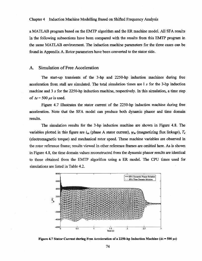
Chapter 4 Induction Machine Modelling Based on Shifted Frequency Analysis
a MATLAB program based on the EMTP algorithm and the ER machine model. All SFA results
in the following subsections have been compared with the results from this EMTP program in
the same MATLAB environment. The induction machine parameters for the three cases can be
found in Appendix A. Rotor parameters have been converted to the stator side.
A. Simulation of Free Acceleration
The start-up transients of the 3-hp and 2250-hp induction machines during free
acceleration from stall are simulated. The total simulation times are 1 s for the 3-hp induction
machine and 3 s for the 2250-hp induction machine, respectively. In this simulation, a time step
of & = 500 ps is used.
Figure 4.7 illustrates the stator current of the 2250-hp induction machine during free
acceleration. Note that the SFA model can produce both dynamic phasor and time domain
results.
The simulation results for the 3-hp induction machine are shown in Figure 4.8. The
variables plotted in this figure are ‘as (phase A stator current), Vm (magnetizing flux linkage), Te
(electromagnetic torque) and mechanical rotor speed. These machine variables are observed in
the rotor reference frame; results viewed in other reference frames are omitted here. As is shown
in Figure 4.8, the time domain values reconstructed from the dynamic phasor results are identical
to those obtained from the EMTP algorithm using a ER model. The CPU times used for
simulations are listed in Table 4.2.
Figure 4.7 Stator Current during Free Acceleration of a 2250-hp Induction Machine (At 500 jts)
74

Chapter 4 Induction Machine Modelling Based on Shifted Frequency Analysis
Table 4.2 CPU Times for Simulations
Free Acceleration Case SFA Model ER Model
3-hp induction machine, T = 1 s, tt = 500 4us 0.728 s 0.556 s2250-hp induction machine, T 3 s, & = 500 ,us 2.43 9 s 1.698 s
* T stands for the total simulation time.
B. Load Torque Change Test
Slow dynamics during step changes in load torque are simulated in this case. The 3-hp
machine originally operates in steady state with no load. A mechanical torque Tm of 12 Nm is
applied at t = 2.05 s. Then Tm is reversed to —12Nm at t = 2.5 s. The simulation time is 3 s with a
Time (s)
Figure 4.8 Dynamic Performance of a 3-hp Induction Machine during Free Acceleration (At = 500 jts)
75

Chapter 4 Induction Machine Modelling Based on Shifted Frequency Analysis
time step of 0.5 ms for the ER model, and a time step of 5 ms for the SFA model. Figure 4.9
shows the phase A stator current and the slip during load torque changes.
Figure 4.9 shows that simulation results from the SFA model with At = 5 ms are as
accurate as those from an EMTP solution with At = 0.5 ms. The CPU time for a 3 s simulation
with the SFA model is 0.266 s, while the simulation with the ER model uses 1.696 s. Therefore,
to achieve the same numerical accuracy, the SFA induction machine model can be more than 5
times faster than its corresponding ER model in this case.
Figure 4.9 Dynamic Performance of a 3-hp Induction Machine during Step Changes in Load Torque (RE At= 0.5 ms, SFA At =5 ms)
C. Three Phase Fault Test
In this simulation of fast transients, the 2250-hp induction machine is first operating
76
2.5Time (s)

Chapter 4 Induction Machine Modelling Based on Shifted Frequency Analysis
under rated conditions with a load torque equal to TB. A 3-phase fault is then applied at the
terminals at t = 6.1 s. After 6 cycles, the fault is cleared. The simulation time is 10 s with a time
step of 500 ps. Figure 4.9 illustrates that the proposed SFA model can simulate fast dynamics of
the machine as accurately as the ER model. The CPU times are 7.258s and 5.562 s for SFA
simulation and ER simulation, respectively.
D. Comparison between SFA and an EMTP Phase-Domain Model
Cases A to C show that the SFA model is as accurate as EMTP phase-domain models for
the same time step i.t. Now we will carefully explore the numerical accuracy and robustness of
Time (s)
Figure 4.10 Simulation Results for a 3-Phase Fault at the Terminals of a 2250-hp Induction Machine (At500 J4s)
77

Chapter 4 Induction Machine Modelling Based on Shifted Frequency Analysis
the SFA model, by using different time steps At in the slow dynamics simulation. The 2250-hp
machine originally operates in steady state with rated torque of 8900 Nm. The machine
dynamics are recorded when a sudden reverse of mechanical torque to -8900 Nm is applied at t
= 6 s. The total simulation time is 10 s.
The SFA model was run with different time steps At = 0.lms, At = lms, At = 5ms, and At
= lOms. The results obtained from an original phase-domain model (refer to p. 142-147 in [43])
with a small At = 0.1 ms are assumed to be the reference accurate time domain results. A
zoomed-in view of phase A stator current is shown in Figure 4.11, which shows that the SFA
model can accurately simulate the system dynamics with a large time step of 10 ms. In fact, even
with a time step of 15 ms, the numerical solution with SFA remains stable. On the contrary, an
EMTP simulation in the time domain with a time step of more than 4 ms became numerically
unstable, as is shown in Figure 4.12.
5.8 6 6.2 6.4 6.6Time (s)
Figure 4.11 Simulation Results by SFA
6.8 / 7.2
78

Chapter 4 Induction Machine Modelling Based on Shifted Frequency Analysis$
Figure 4.12 Time Domain Results from an EMTP Algorithm Implemented in MATLAB
Table 4.3 summarizes the CPU times needed for the SFA and ER simulations in this case.
It can be seen that the SFA model was about 10 times faster (0.370 s vs 2.80 1 s) than the EMTP
phase-domain model (ER model) to achieve a comparable accuracy. In certain situations, for
instance, when simulating a system with power electronics components, an EMTP-type
simulator may have to use very small time steps, for example, less than 0.1 ms. As can be seen
from Table 4.3 that a SFA model with zt = lOms can be about 75 times faster than an EMTP
model with & = 0.lms, for reasonable accuracy. Therefore, it is very promising to apply the SFA
model in hybrid simulators, where the power electronics components as well as the network can
be simulated with a small time step, while the SFA can be used for machine models with a larger
time step. Further, the new SFA model has the capability to be extended to model the saturation
and deep bar effects in induction machines. The SFA modeling framework is shown to be
successful for machine modeling as a new method, which opens the door for more future
research such as applying the SFA to wind turbine generator modeling, and developing SFA
based EMTP simulators or hybrid simulators, and so on.
Table 4.3 CPU Times for Simulations
2250-hp induction machineSFA Model ER Model
Torque Change CaseT=lOs,&0.lms 36.108 s 27.328sT=lOs,&=lms 3.725s 2.801sT=lOs,&5ms 0.738s --
T= 10 s, & = 10 ms 0.370 s* Numerically unstable.
79

Chapter 4 Induction Machine Modelling Based on Shifted Frequency Analysis
4.4 Summary
(1) An Equivalent-Reduction-based induction machine model is proposed. With a lower
number of model equations, it is actually a full-order phase-domain model but is simpler and
faster. Park’s transformation is implicitly used in the ER model in order to maintain the elegance
and simplicity in the discrete-time equivalent circuit. As a non-ad hoc approach, the ER can also
be used for building more efficient models for other power system elements.
(2) Based on the ER model, a SFA model is proposed as a general-purpose model capable of
simulating both fast transients and slow dynamics. Case study results have confirmed the SFA
induction machine model is a valuable component for real-time EMTP simulations. It is
observed that the SFA model is in excess of 70 times faster than the EMTP solution with the RE
model when simulating dynamics with frequency spectra close to the fundamental power
frequency.
80

Chapter 5 EMTP Implementation
Chapter 5
EMTP Implementation
5.1 Introduction
Since a number of power system component models in the shifted frequency domain
have been built in the previous chapters, it is now time to ask how they can be used in a general
purpose simulation tool based on the Shifted Frequency Analysis.
EMTP, which was originally developed for calculating the transient overvoltages in
transmission systems, has been significantly expanded to tracing the evolution of the system
states in arbitrary multi-phase power networks consisting of all types of components. With
improved functionality, accuracy and numerical stability, EMTP has become a standard tool
being widely used in the power industry for system planning and designing purposes. Now
EMTP is seeing broader applications in power system steady state [58] and dynamics studies and
will remain one of the mainstreams in power system research. The intention of this thesis is to
expand EMTP to efficiently simulate the slow dynamics in power systems, and to bridge the gap
between the EMTP and a unified power system analysis tool. This means that the EMTP
algorithm will be adopted in the SFA-based simulation tool. What makes a difference here is that
the electrical variables are described by dynamic phasors instead of instantaneous time values.
81

Chapter 5 EMTP Implementation
5.2 Program Structure
The implicit trapezoidal rule of integration, which has attractive characteristics in terms
of accuracy and numerical stability, is used in EMTP and is followed in the SFA-based
modelling of system components. By using the trapezoidal rule, the differential equations
representing all network components are converted into algebraic relationships which can be
interpreted as equivalent resistances or admittances, voltages, currents, and known history terms.
Then the nodal equations of the system can be written directly as follows.
[G][V(t)] = [I(t)]+ [H(t)] (5.1)
where
[G] is the matrix of the nodal equivalent admittances
[VQ)] is the vector of the nodal voltages, which are dynamic phasors
[1(t)] is the vector of the nodal currents, which are dynamic phasors
[11(t)] is the vector of the nodal history terms
The voltages of the nodes connected to voltage sources are known quantities, therefore
the corresponding equations can be eliminated. Suppose A is the index set denoting the nodes
with unknown voltages, and B is the index set for nodes with known voltages, then the nodal
equations can be written in a block matrix form
rGM G1EvA(t)1 = EIA(tHAt)1 (5.2)[GBA GBB][VB(t)J [IB(t)+HB(t)]
Thus the unknown voltages can be obtained at time t by solving the following equations
GVA(t) [IA(t) + HA(t)]—GVB(t) (5.3)
In this thesis, a toolbox for simulating power system dynamics in the shifted frequency
domain has been developed with MATLAB. This dynamic phasor tool consists of several files,
which are depicted in the schematic structure in Figure 5.1.
A. Input Data File
Input data file provides the data needed for the simulation of a multi-phase power
network. These include transmission line data, load data, machine data, switching operations
82

Chapter 5 EMTP Implementation
data, voltage sources data, etc. All these data are documented in a MATLAB script file and most
of the data are provided as the MATLAB arrays. Refer to Appendix C for the input data format.
System Solver Main.m
PiLineParameters.m
MacParameters.m
Data Processing LoadParameters.m
RLCParameters.m
EMTP Dynamic PhasorSimulation Tool
(EMTDP)
EquivalentAdmittance Matrix Gsys.m
Forming
Updating UpdateG.m
Admittance Matrixand History Terms UpdateHist.m
Data Input File Case_i 3Bus.m
Figure 5.1 Schematic Structure for the EMTP Dynamic Phasor Simulation Tool
B. Data Processing Files
When the input data are read by the main program, the data processing functions are
called to establish the equivalent circuit for different power system components, and initialize
their history terms for the simulation at the first time step. The equivalent circuit for different
components can be found in previous chapters.
The initialization in the SFA simulations is based on the snapshot method. First, let the
dynamic phasor program run with zero initial conditions and reaches the steady state. Then, a
snapshot of.the system is taken by saving system variables and history terms at a particular time
step. These system variables and history terms from the snapshot file are fed to the SFA program
as the initial conditions. With system variables and history terms initialized, the SFA simulation
83
Chapter 5 EMTP Implementation
will run with a ‘flat’ start, and the advantage of using large time step in simulating 60 HZ
dynamics is achieved.
C. File for Building G Matrix
The file ‘Gsys.m’ builds the system [G] matrix in equation (5.1) and returns the [Gj
and [Gp.i] to the system solver for calculating the unknown voltages. The following explains
how this simulation tool inserts power system components into equivalent admittance matrix [G]
by taking the it-circuit model of a transmission line as an example.
Suppose there is a three-phase it-circuit for a transmission line connecting node set J
(=[ji, j2, j3}) and node set K (=[k1,k2,k3]) as depicted in Figure 5.2. As can be seen in Figure 5.2,
the it-circuit model consists of a coupled RE branch and two coupled capacitances. When
discretized by the trapezoidal rule, the coupled RE branch will contribute a 3 x3 equivalent
admittance matrix to [G], and contributes a 3x1 history term hpj to [H]. Similarly, the
coupled capacitances will also contribute a 3 x 3 equivalent admittance matrix Gc and a 3 xl
history term hc. From equations (2.21) and (2.24), it can be found that GRL will be entered into
[G]j,j and [G]jçK in the system admittance matrix [G], and —G1j. into [G]J,K and [G]jçj. For
instance, G(ll) will be added to the element Ggi(1,2) will be added to [GJJ1i2, GII(l,2)to
[G]13, GRI(2,1) to [G]j21, and so on. This procedure is illustrated in Figure 5.3. The MATLAB
implementation of this process is shown in Figure 5.4.
This routine also moves the nodes connecting to the voltage sources to the bottom of the
system equation set, and then extract the sub-blocks [Gj and [Gpj] from [G].
C13
Figure 5.2 The fl Transmission Line Model
84

Chapter 5 EMTP Implementation
D. File for Updating [G] and [H]
The MATLAB files UpdateG.m will update the G matrix when changes happen in the
network configuration, e.g. line tripping or faults. The file UpdateHist.m will calculate the
history terms at each time step and return them to the solver for calculating unknown variables.
E. System Solver
The system solver Main.m is the core function in the simulation tool. In each time step,
this routine assembles the right hand side of (5.3), performs downward operations on it, and does
the back-substitution to obtain the unknown nodal voltages. After the unknowns are found, the
routines for updating history terms and/or admittance matrix are called, in preparation for the
calculations at the next step. The simulation run will continue until the total simulation time is
reached. A schematic flow chart of the system solver is presented in Figure 5.5.
111213 k1k2k3
\+Gc
+G -G\___ --- /
/-G +G
+ G1
[Gj [hj
Figure 5.3 Contributions of the fl-Circuit Transmission Line Model to the Nodal Admittance Matrix
3233
k1Ic2k3
jl32
33
k1Ic2Ic3
+ hcj
/hRL
+ hc K
85
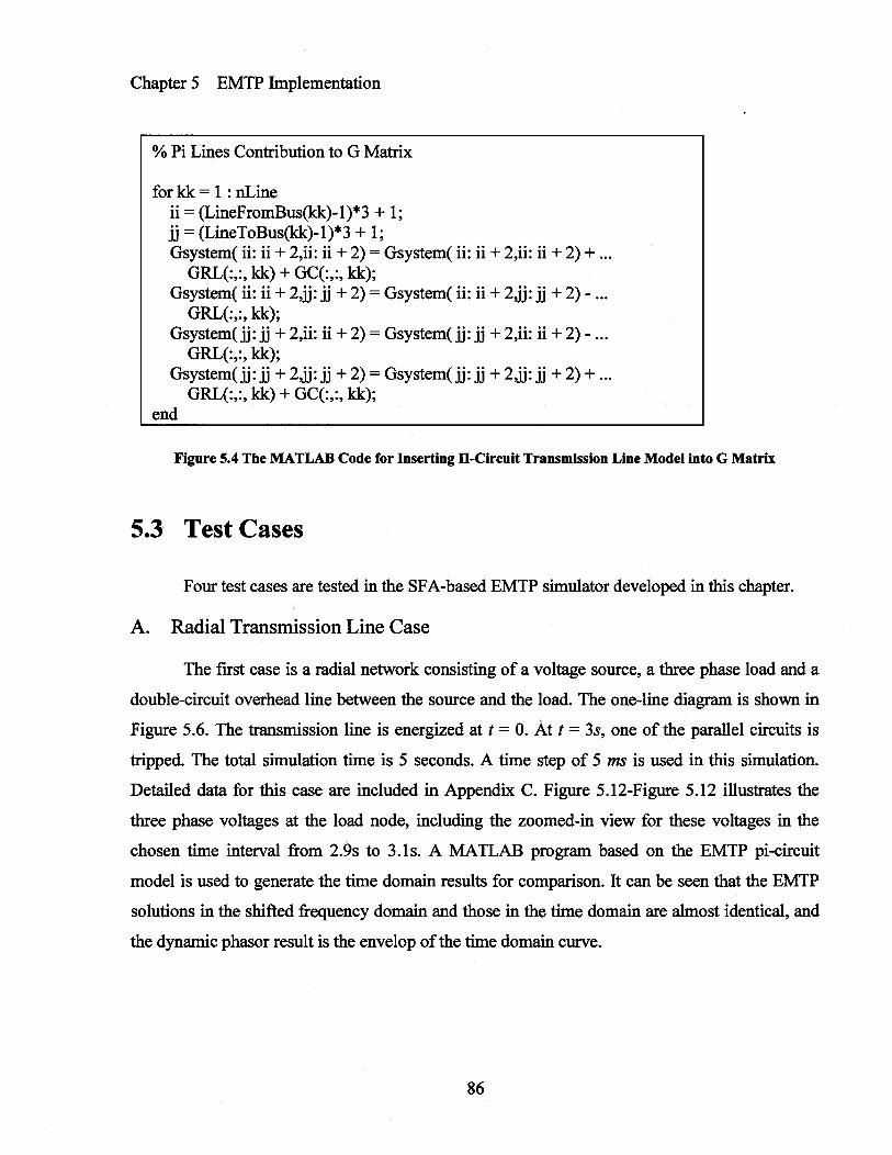
Chapter 5 EMTP Implementation
% Pi Lines Contribution to G Matrix
for kk = 1: nLineii = (LineFromBus(kk)- 1 )*3 + 1;jj = (LineToBus(kk)1)*3 + 1;Gsystem( ii: ii + 2,11: ii + 2) = Gsystem( ii: ii + 2,ii: ii + 2) +
GRL(:,:, kk) + GC(:,:, kk);Gsystem( ii: ii + 2,jj: jj + 2) = Gsystem( ii: ii + 2,jj: jj + 2) -
GRL(:,:, kk);Gsystem( jj: jj + 2,11: ii + 2) = Gsystem( jj: jj + 2,ii: ii + 2) -
GRL(:,:, kk);Gsystem(jj: jj + 2,jj:jj + 2) = Gsystem(jj:jj + 2,jj:jj + 2) +
GRL(:,:, kic) + GC(:,:, kk);end
Figure 5.4 The MATLAB Code for Inserting H-Circuit Transmission Line Model into G Matrix
5.3 Test Cases
Four test cases are tested in the SFA-based EMTP simulator developed in this chapter.
A. Radial Transmission Line Case
The first case is a radial network consisting of a voltage source, a three phase load and a
double-circuit overhead line between the source and the load. The one-line diagram is shown in
Figure 5.6. The transmission line is energized at t = 0. At t = 3s, one of the parallel circuits is
tripped. The total simulation time is 5 seconds. A time step of 5 ms is used in this simulation.
Detailed data for this case are included in Appendix C. Figure 5.12-Figure 5.12 illustrates the
three phase voltages at the load node, including the zoomed-in view for these voltages in the
chosen time interval from 2.9s to 3.ls. A MATLAB program based on the EMTP pi-circuit
model is used to generate the time domain results for comparison. It can be seen that the EMTP
solutions in the shifted frequency domain and those in the time domain are almost identical, and
the dynamic phasor result is the envelop of the time domain curve.
86

Chapter 5 EMTP Implementation
( Input Data
Find Steady State Solution to InitializeHistory Terms and Variables at I =
Jr
Build GAA, GAB for Transient Solution
1.Factor G into LU Form
JrStart Time Step Simulation
=
Evaluate Current and Voltage Sources,
__________
Update the Right Hand Side of(5.3)
J,N
I=t+Ai
Perform Downward Operations on RHS of(5.3),Do Back-substitution to Solve Nodal Voltages
‘I,Update History Terms
R,XLoad
Any Switching ‘‘ Modify and
Output Results
Figure 5.5 Flow Chart for Dynamic-Phasor-Based EMTP Simulator
Source Busi Bus2
Figure 5.6 One-line Diagram of a Radial Test System
87

Chapter 5 EMTP Implementation
‘C I
0 0.5 1 1.5 2 2.5 3 3.5 4 4.5 5Time (s)
Figure 5.9 Phase B Voltage at the Load Node (At = 5 ms)
88
SFA Solution‘nfl
—l
0.5 1 1.5 2 2.5 3 3.5 4 45 5Time (s)
Figure 5.7 Phase A Voltage at the Load Node (At = 5 ms)
Figure 5.8 Zoomed-in View of Phase A Voltage at the Load Node (At = S ms)
‘ r 1
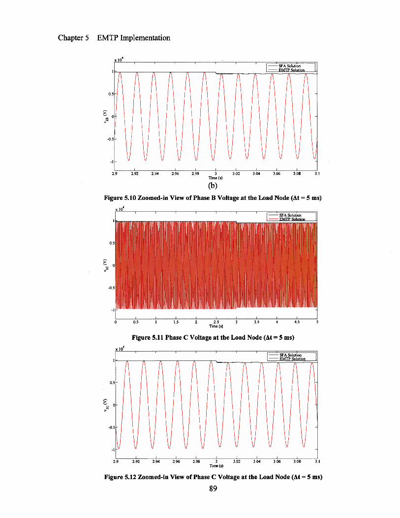
Chapter 5 EMTP Implementation
0.5
>
>
-0.5
Li
—1
,i i
2.9 2.92 2.94 2.96 2.98Time(s)
(b)
3.02 3.04 3.06 3.08 3 1
0 0.5 I 1.5 2 2.5 3 3.5 4 4.5 5Time (s)
Figure 5.11 Phase C Voltage at the Load Node (At =5 ms)
xI I I
SFA SolutionEMTP Solution
0.5
0
-0.5
—l
2.9 - 2.92 2.94 2.96 2.98 3 302 3.04 3.06 108 3.1Time (s)
Figure 5.12 Zoomed-in View of Phase C Voltage at the Load Node (At = 5 ms)
89
I I I I I I .1SFA Solution
Figure 5.10 Zoomed-in View of Phase B Voltage at the Load Node (At = 5 ms)
x
___________
1
IVVVVV\IVVVVV
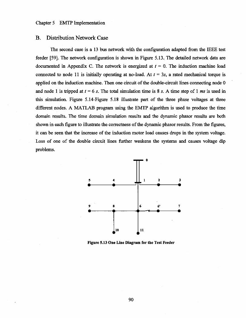
ChapterS EMTP Implementation
B. Distribution Network Case
The second case is a 13 bus network with the configuration adapted from the IEEE test
feeder [59]. The network configuration is shown in Figure 5.13. The detailed network data are
documented in Appendix C. The network is energized at t = 0. The induction machine load
connected to node 11 is initially operating at no-load. At t = 3s, a rated mechanical torque is
applied on the induction machine. Then one circuit of the double-circuit lines connecting node 0
and node 1 is tripped at t = 6 s. The total simulation time is 8 s. A time step of 1 ms is used in
this simulation. Figure 5.14-Figure 5.18 illustrate part of the three phase voltages at three
different nodes. A MATLAB program using the EMTP algorithm is used to produce the time
domain results. The time domain simulation results and the dynamic phasor results are both
shown in each figure to illustrate the correctness of the dynamic phasor results. From the figures,
it can be seen that the increase of the induction motor load causes drops in the system voltage.
Loss of one of the double circuit lines further weakens the systems and causes voltage dip
problems.
5 4
0
1 2 3
11•
Figure 5.13 One Line Diagram for the Test Feeder
90

ChapterS EMTP Implementation
>
Figure 5.15 Zoomed-in View of Phase A Voltage at the Induction Machine Node (At = 1 ms)
3 3.5 4 45 5 5.5 6 6.5 7 7.5 8Time (s)
Figure 5.16 Phase B Voltage at Load Node 6 (At = 1 ms)
91
— SFA Solution
EMTP Solution
3 3.5 4 4.5 5 5.5 6 6.5 7 7.5Time (s)
Figure 5.14 Phase A Voltage at the Induction Machine Node (At = 1 ms)
I
SFA SolutionEMTP Solution
I I I I I I I I
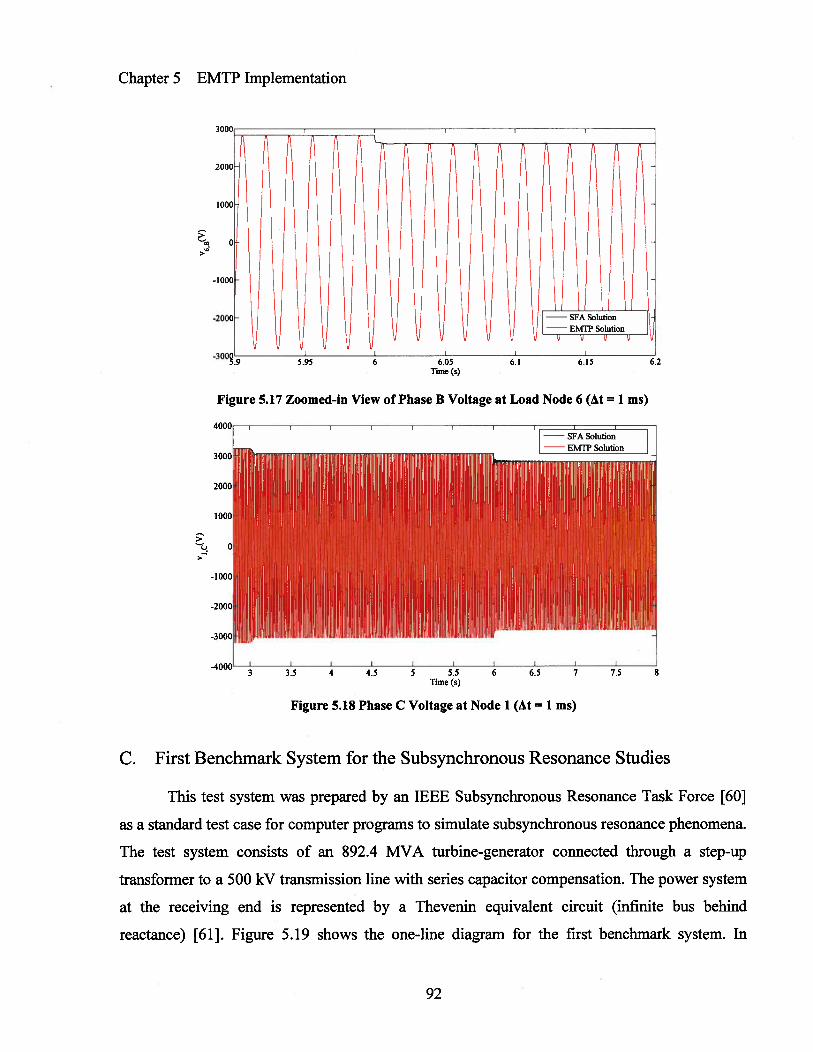
Chapter 5 EMTP Implementation
>
I I I I I
3.5 4 4.5 5 5.5 6Time (s)
Figure 5.18 Phase C Voltage at Node I (At = 1 ms)
C. First Benchmark System for the Subsynchronous Resonance Studies
This test system was prepared by an IEEE Subsynebronous Resonance Task Force [601
as a standard test case for computer programs to simulate subsynchronous resonance phenomena.
The test system consists of an 892.4 MVA turbine-generator connected through a step-up
transformer to a 500 kV transmission line with series capacitor compensation. The power system
at the receiving end is represented by a Thevenin equivalent circuit (infinite bus behind
reactance) [61]. Figure 5.19 shows the one-line diagram for the first benchmark system. In
Figure 5.17 Zoomed-in View of Phase B Voltage at Load Node 6 (At = 1 ms)
SFA SolutionEMTP Solution
.4OQO6.5
92

Chapter 5 EMTP Implementation
Figure 5.19, all data are represented in p.u. based on 892.4 MVA and 500 kV. The generator
parameters of the electrical part are listed as below
Xci = 1.79 p.U. Xq 1.71 p.U. Ra= 0
X’d = 0.169 p.U. X’q = 0.228 p.U. X1 0.13 p.U.
X”d = 0.135 p.U. X”q = 0.2 p.u. f 60 Hz
T’cio = 4.3 S T’qo 0.85 S it(O) = 1 f.U.
T”do 0.032 S T”qo = 0.05 5
The original purpose of this case was to simulate the interaction between the mechanical
torque placed on the generator turbines and the electrical torque related to the power network,
and the resulting shaft torsional oscillations. Accordingly, a detailed multi-mass modcl of the
mechanical shaft is adopted in [601, [611, where the generator shaft system is modeled by 6
masses including 4 turbine sections HP, IP, LPA and LPB, 1 generator and 1 exciter. This thesis
focuses on the feasibility of applying the SFA method, and thus uses a simpler single-mass
representation of the mechanical part. The total inertia constant of the turbine and generator is
2.894 seconds. The SFA synchronous machine model in Chapter 3 is used in this test case. It
should be noted that the SFA synchronous machine model of Chapter 3 can be extended to
model the multi-mass shaft system by adding differential equations for individual spring-masses
to the differential equations of the shaft system. The self and mutual damping effect can also be
easily included in the shaft system equations.
The detailed network parameters can be found in [601 and [611.
26kV/500kV A R1 0.02 X1 = 0.50B X1 = 0 06
R0=0.50 X0=l.56 —
IGenerator = 0.14 —
Infinite Bus
X0=0.14 Xc-O.371 X=0.04
10 = 0.04
Figure 5.19 The First Benchmark Network for Subsynchronous Resonance Studies
93

Chapter 5 EMTP Implementation
In this test, a three-phase fault occurs at bus B at t = 3 s. After 4 cycles, the fault is
cleared. The total simulation time is 3.5 s. A time step of 1 ms is used in this simulation. The
whole system is represented using the SFA models proposed in the previous chapters. The
generator terminal voltages, the voltages at bus A and bus B, and the voltages across the series
capacitors are monitored during the SFA simulation. Figure 5.20 to Figure 5.23 illustrate the
dynamic phasor results for the system voltages at different locations as well as the time domain
results transformed back from the corresponding dynamic phasors. The dynamic phasor results
show that, after the fault is applied and cleared, there are low frequency oscillations happening at
the generator terminals, on the transformer sides, and across the series capacitor banks.
‘U
‘U
C
C
‘UF
CC‘UC‘U
time (s)
Figure 5.20 Generator Terminal Voltage: Phase A (At = 1 ms)
94

Chapter 5 EMTP Implementation
0
0
.0
I
Figure 5.21 Transformer High Side (Bus A) Voltage: Phase A (At = 1 ms)
Figure 5.22 Voltage across Series Capacitor: Phase A (At = 1 ms)
These oscillations are an electrical phenomenon because the shaft system is modeled as a
single mass. The slow oscillations are caused by resonances with the series capacitor, which are
excited by the fault and the switching operations. The resonance mode(s) is determined by the
inherent characteristics of the power network. In fact, the modes or natural frequencies can be
quantitatively found by either performing a frequency scan (steady-state solutions over a
frequency range) or by calculating the eigenvalues of the admittance matrix of the electrical
95
3time (s)

Chapter 5 EMTP Implementation
network. Similar to the network resonance analysis, if the shaft system is represented by the
detailed multi-mass model, we can also determine the torsional natural frequencies (eigenvalues)
and mode shapes (eigenvectors) by applying the modal analysis to the shaft differential
equations. If the complement of the natural frequency of the network is close to one of the
torsional frequencies of the shaft system, torsional oscillations will be excited [331. This is the
mechanism of the subsynchronous resonance. The dynamic phasor results obtained from the
SFA simulations show that the oscillations with frequencies around 30 Hz have been excited in
this benchmark system. On the other hand, the natural frequencies of the 6-mass shaft system
were found to be 15.71 Hz, 20.21 Hz, 25.55 Hz, and 32.28 Hz [601. That means the complement
of the natural frequency of the series-compensated network is close to the torsional natural
frequencies, which would result in a subsynchronous resonance in this system and would build
up torsional oscillations on the shaft. This has been verified by EMTP simulations [611.
In summary, the SFA simulations are able to capture the slow oscillations in the
benchmark system and can be used for subsynchronous resonance studies once the detailed shaft
model is incorporated into the SFA synchronous machine models.
U,
0>U,0
0to
D. Second Benchmark System for the Subsynchronous Resonance Studies
Eight years after the first subsynchronous resonance benchmark was published, the IEEE
Subsynchronous Resonance Working Group proposed a second benchmark [621. The second
96
time (s)
Figure 5.23 Infinite Bus (Bus B) Voltage: Phase A (At = 1 ms)

Chapter 5 EMTP Implementation
benchmark is a case consisting of a 600 MVA generator connected through a step-up transformer
to two parallel lines, one of which is series compensated. The compensation rate of the line is
55%. The power system at the receiving end is represented by a Thevenin equivalent circuit
(infinite bus behind impedance). Figure 5.24 shows the one-line diagram for the second
benchmark system. All data in Figure 5.24 are represented in p.u. on a 100 MVA, 500kV base.
The mechanical part of the round rotor turbine generator is again represented as a single-mass
model with a total inertia of 2.683 seconds in the SFA simulation. In [621, a more detailed multi-
mass representation is used with 4 masses. The parameters of the electrical part are based on the
machine ratings, which are given below.
Xd = 1.65 p.U. Xq = 1.59 p.u. Ra = 0.0045 3.U.
X’d = 0.25 p.u. X’q = 0.46 p.U. Xi = 0.14 p.U
X”d = 0.20 p.U. X”q = 0.20 p.u. f 60 Hz
T’do = 4.5 S T’qo = 0.55 S if(O) = 1 3.U.
Tdo = 0.04 S T”qo = 0.09 s number of poles = 2;
The detailed benchmark network parameters can be found in [62] and [61].
In this test, a three-phase fault is applied at the high voltage side of the transformer
connecting to bus 2 at t = 3 s. The fault clearing time is 1 cycle, and the total simulation time is
3.5 s. The time step used in this simulation is 1 ms. Figure 5.25 to Figure 5.28 show the dynamic
phasor results for the system voltages at different locations together with the time domain results
transformed back from the corresponding dynamic phasors. Obviously, oscillations slower than
the fundamental frequency are excited in the system after the fault occurs, which can be seen
from the dynamic phasors of the generator terminal voltage, the transformer high side voltage
and the voltage across the series capacitor. Note that bus 1 does not see large deviations in the
voltage because it is electrically close to the infinite external system, and also because the series
capacitor is acting as a highpass filter that blocks the slow oscillations in the system. The test
results on the second benchmark system further verify that the SFA method can capture the so
called ‘parallel resonance’ phenomenon [62] in the meshed power system.
Note that relatively small time-step is used for the simulation of the subsynchronous
resonance because large frequency deviation occurs after the fault is applied. The reason why a
small time step has to be used is that large frequency deviation defines a wide bandwidth in the
shifted frequency domain, which in turn requires smaller time steps to respect the Nyquist
97

Chapter 5 EMTP Implementation
frequency limit in the shifted frequency domain. This indicates that a variable time step scheme
is a future research direction to realize full potential of the SFA method. The time step can be
reduced when system states are changing rapidly in order to achieve better accuracy in the SFA
simulation. On the other hand, when system dynamics slowdown, large time steps can be used to
avoid unnecessarily long computational time while still achieving reasonable accuracy.
Generator
R=0.0002X=0.02
Bus 2
R1 = 0.0067R0=0.0186
R1 = 0.0074R00.022
Xi = 0.0739X0=0.21
Bus 1
Xi = 0.08X0=0.24
Bus C
Xiijne
Ri =R0=0.0014
X1 = X0= 0.03
Infinite Bus
Figure 5.24 The Second Benchmark Network for Subsynchronous Resonance Studies
98

Chapter 5 EMTP Implementation
VC:
-C
V
C:
C>
I
VC:C:
-C
V
C
C
UCt
UC:V
VC’)
Figure 5.25 Generator Termiual Voltages: Phase A (At = 1 ms)
Figure 5.26 Voltage across Series Capacitor: Phase A (At = 1 ms)
time (s)
3time (s)
99

Chapter 5 EMTP Implementation
0
•0CD
I
I
>
0
ci,
0
Figure 5.27 Transformer High Side (Bus 2) Voltage: Phase A (At = 1 ms)
Figure 5.28 Infinite Bus (Bus 1) Voltage: Phase A (At = 1 ms)
The test results from all the above cases indicate that the dynamic phasor is a
generalization of the phasor concept, which can represent the dynamic waveform in power
systems, without loss of important information. The SFA method with its implementation in the
EMTP environment can integrate the differential equations of the power system in the SFA
domain and can produce dynamic phasors for electrical variables, which are visually clear and
100
2.5time (s)

Chapter 5 EMTP Implementation
easy to follow for power engineers. With the SFA method, power engineers may gain better
insight into the EMTP simulation results, and we would expect broader applications of the
EMTP in power system steady state and dynamics studies, beyond the fast transient simulations.
101

Chapter 6 Conclusions
Chapter 6
Conclusions
6.1 Summary of Contributions
The goal of this thesis is to extend EMTP functionality for power system dynamic
simulation, especially for simulating dynamics with frequency spectra close to the fundamental
power frequency. This has been accomplished by developing the Shifted Frequency Analysis
(SFA) method, modeling system components with SFA, and accelerating the EMTP simulations
for dynamics around 60Hz. A series of contributions made in this thesis are the following.
I. The theory of Shifted Frequency Analysis is proposed with the help of Hubert transform
and analytic signal concept. Numerical accuracy analysis is performed for the discrete-
time SFA simulation.
II. Linear circuit components, transformer, exponential load and steady-state induction
motor are modeled in the shifted frequency domain.
III. An efficient SFA-based synchronous machine model for the simulation of slow system
dynamics is developed. This model is a general-purpose model that can be used for
evaluating the dynamic performance of both the salient-pole and the cylindrical-rotor
machines.
IV. The SFA method is extended to model the induction machines. This thesis proposes a
new phase-domain induction machine model based on the equivalent-reduction (ER)
approach. The ER model has a concise discrete-time equivalent circuit that can be
directly incorporated into EMTP-type simulators. Based on the ER model, a SFA
induction machine model is proposed as a general purpose model capable of simulating
both fast transients and slow dynamics.
V. An EMTP simulation tool based on the SFA is developed. Simulation results
102

Chapter 6 Conclusions
validate that the SFA method is capable to efficiently simulate power system fundamental
frequency dynamics. This is the first practical accomplishment to build a unified power
system analysis tool based on the EMTP solution.
6.2 Future Research
The accomplishment achieved in this thesis will inspire researchers to apply SFA and
associated techniques to power system analysis and other potential areas. The success of the
applications of SFA may be achieved in different aspects such as:
Apply the SFA to the modeling and analysis of renewable energy resources, dispersed
generation plants, and industrial power systems. In the foreseeable future, more and more
independent-power-producer-owned (IPP-owned) generation units will be connected into
the power transmission and distribution system due to a deregulated electricity market.
Many of these plants will be cleaner, and many of them will be renewable energy sources
such as biomass, solar, wind, geothermal, small hydro, ocean energy, and so on. The IPP
interconnection impact studies, which identify the system constraints brought about by
the integration of IPPs, and determine network upgrades and remedial action schemes,
are therefore critical for the reliable and safe operation of the TPPs and associated power
systems. By applying the SFA technique in the IPP modeling, it may lead to accurate and
efficient solutions in the IPP impact study, which is hardly achievable with the current
phasor tools.
II. Develop new component models and controller models, and improve the SFA-based
EMTP solver. In addition, the future SFA simulator will adopt more object-oriented
design such that each module for new components can simply ‘plug into’ the simulation
engine without modifying the core codes. The robustness and efflciency of the core codes
will also be improved by using up-to-date sparsity techniques.
III. The equivalent-reduction idea can be used for building more efficient models for various
types of machines, transformers and power system equipments, as long as they can be
mathematically represented by differential equations with mutually coupled state
variables. These new models can then be further explored in the shifted frequency
domain.
103

Chapter 6 Conclusions
IV. Transform the SFA-based simulation tool into parallel programs. The UBC Object
Virtual Network Integrator (OVNI) [631 is a real time parallel simulator, which uses PC
clusters [64] as hardware and Muti-Area Thevenin Equivalent (MATE) algorithm as
solution engine [65]-[69]. MATE partitions the power system into subsystems and solves
them in parallel. By changing the real-valued component models to the dynamic phasor
models, a new OVNI simulator based on SFA can be implemented. In the future, one
may expect this new simulator to serve as a distributed simulation tool for the supervision
and control of self-healing power infrastructures.
V. Further investigate the basic theory of the SFA method. This will still be an interesting
field in future research. There are two limitations in the current SFA method. First, SFA
simulation is computationally more expensive than EMTP simulation for the same
integration step At. This is due to the higher computational cost of operating with
complex numbers in SFA as compared to real numbers in EMTP and also to the
computational cost involved in transferring between shifted frequency domain and time
domain. Second, the aliasing effect may occur when simulating very fast transients in a
system [24]. This may introduce error or distortion in SFA simulation result. Some new
theories such as discrete-time analytic signal, Hilbert-Huang transform, and new
antialiasing techniques are likely to bring theoretical breakthroughs and may lead to the
next generation SFA method, which may be more flexible and accurate than the current
SFA.
VI. It may be worthwhile to look into transformations to d,q,0-quantities as an alternative to
dynamic phasors [70], particularly for cases where the three-phase impedances are
balanced, and where the faults are symmetrical three-phase faults.
VII. Last but not least, the applications of the SFA method is not limited to the EMTP
solution. The Shifted Frequency Analysis can also be introduced into any other circuit
simulators, for instances, some state-space-based circuit and/or electric machinery
solvers, SPICE, and so on. It is equally suitable to be implemented in the variable time
step simulators such as Simulink®. It can also be used in hybrid simulations, and
hardware-in-loop simulators.
All in all, the SFA is believed to have opened new doors of opportunity for research
relating to dynamic simulations, and further theoretical work and applications are justified.
104

Bibliography
Bibliography
[1] U.S.-Canada Power System Outage Task Force, Final Report on the August 14, 2003
Blackout in the United States and Canada: Causes and Recommendations, Apr. 2004.
[2] G. T. Heydt, C. C. Liu, A. G. Phadke, V. Vittal, “Solution for the Crisis in Electric Power
Supply,” IEEE Computer Applications in Power, vol. 14, no. 3, pp. 22-30, Jul. 2001.
[3] IEEE/CIGRE Joint Task Force on Stability Terms and Definitions, “Definition and
Classification of Power System Stability,” IEEE Transactions on Power Systems, vol. 19, no.
3,pp. 1387- 1401,Aug.2004.
[4] W. Li, Risk Assessment of Power Systems: Models, Methods, and Applications, New York:
IEEE Press and Wiley & Sons, 2005.
[5] S. R. Aumuri, L. R. Malone, V. Burtnyk, “Representation of Single-Pole Open Conditions in
Stability Studies”, IEEE Transactions on Power Systems, vol. 6, no. 1, pp 9-15, Feb. 1991.
[6] V. Ajjarapu, C. Christy, “The Continuation Power Flow: a Tool for Steady State Voltage
Stability Analysis”, IEEE Transactions on Power Systems, vol. 7, no. 1, pp 416-423,
February 1992.
[7] T. Van Cutsem, C.Voumas, Voltage Stability of Electric Power Systems, Kluwer Academic
Publishers, 1998.
[8] IEEE/PES Power System Stability Subcommittee, Voltage Stability Assessment: Concepts,
Practices and Tools, Final Document, Aug. 2002.
[9] H. W. Dommel, EMTP Theory Book, 2nd edition, Vancouver, BC: MicroTran Power System
Analysis Corporation, 1996.
[10] H. W. Dommel, “Digital Computer Solution of Electromagnetic Transients in Single- and
Muti-Phase Networks,” IEEE Transactions on Power Apparatus and Systems, vol. 88, no. 2,
pp. 734-771, Apr. 1969.
105

Bibliography
[11] MicroTran Power System Analysis Corporation, MicroTran Reference Manual:
Transients Analysis Program for Power and Power Electronic Circuits, Vancouver, BC,
Canada, 2002.
[121 Manitoba HVDC Research Center, User’s Guide of PSCAD, Winnipeg, Manitoba,
Canada, 2003.
[13] Canada/America EMTP Users Group, ATP Rule Book, 1998.
[14] J. Mahseredjian, S. Dennetiere, L. Dube, B. Khodabakhchian, and L. Gerin-Lajoie, “On a
New Approach for the Simulation of Transients in Power Systems,” Electric Power Systems
Research, vol. 77, no. 11, pp. 15 14-1520, 2007.
[15] DIgSILENT GmbH, DlgSlLENTPowerFactory V13 User Manual, 2005.
[16] RTDS Technologies, Real Time Digital Simulator User Manual, 2003
[17] C. Henville, R. Folkers, A. Hiebert and R. Wierckx, “Dynamic Simulations Challenge
Protection Perfonnance,” Proceedings of the 30th Western Protective Relay Conference,
Spokane, WA, Oct. 2003.
[18] V. Venkatasubramanian, “Tools for Dynamic Analysis of the General Large Power
System Using Time-Varying Phasors,” International Journal ofElectrical Power and Energy
Systems, vol. 16, no. 6, pp. 365-376, Dec. 1994.
[19] M. Stubbe, A. Bihain, J. Deuse, J. C. Baader, “STAG-A New Unified Software Program
for the Study of the Dynamic Behaviour of Electrical Power Systems”, IEEE Transactions on
Power Systems, vol. 4, no. 1, pp 129-138, Feb. 1989.
[20] S. Henschel, “Analysis of Electromagnetic and Electromechanical Power System
Transients with Dynamic Phasors,” Ph. D. dissertation, The University of British Columbia,
Vancouver, Canada, 1999.
[21] A. M. Stankoviá, T. Aydin, “Analysis of Asymmetrical Faults in Power Systems Using
Dynamic Phasors,” IEEE Transactions on Power Systems, vol. 15, no. 3, pp. 1062-1068, Aug.
2000.
[22] A. M. Stankoviá, S. R. Sanders, T. Aydin, “Dynamic Phasors in Modeling and Analysis
of Unbalanced Polyphase AC Machines,” IEEE Transactions on Energy Conversion, vol. 17,
no. l,pp. 107-113, Mar. 2002.
106

Bibliography
[23] A. M. Stankovié, B. C. Lesieutre, T. Aydin, “Modeling and Analysis of Single-Phase
Induction Machines with Dynamic Phasors,” IEEE Transactions on Power Systems, vol. 14,
no. 1, pp. 9-14, Feb. 1999.
[24] J. R. Marti, “Shifted Frequency Analysis (SFA) for EMTP Simulation of Fundamental
Frequency Power System Dynamics”, Internal Report, Power System Laboratory, The
University of British Columbia, Vancouver, Canada, Apr. 2005.
[25] 5. L. Hahn, Hubert Transforms in Signal Processing, Norwood, MA: Artech House,
1996.
[26] A.V. Oppenheim and A. S. Wilisky, Signal and Systems, Upper Saddle River, NJ:
Prentice-Hall, 1996.
[27] R. Shintaku and K. Strunz, “Branch Companion Modeling for Diverse Simulation of
Electromagnetic and Electromechanical Transients,” IPST’OS, Montreal, Canada, Jun. 2005.
[28] P. Zhang, J. R. Marti, H. W. Dommel, “Synchronous Machine Modelling Based on
Shifted Frequency Analysis,” IEEE Transactions on Power Systems, vol. 22, no. 3, pp. 1139-
1147, Aug. 2007.
[29] P. Zhang, J. R. Marti, H. W. Dommel, “Induction Machine Modelling Based on Shifted
Frequency Analysis,” IEEE Transactions on Power Systems, Accepted for Publication.
[30] J. R. MartI, J. Lin, “Suppression of Numerical Oscillations in the EMTP,” IEEE
Transactions on Power Systems, vol. 4, no. 2, pp. 739-747, May 1989.
[31] L. W. Ehrlich, “Complex Matrix Inversion Versus Real,” Communications of the ACM
vol. 13, no. 9, pp. 561-562, Sept. 1970.
[32] L. Tornheim, “Inversion of a Complex Matrix,” Communications of the ACM, vol. 4,
issue 9, pp. 398, Sept. 1961.
[33] P. Kundur, Power System Stability and Control, New York: McGraw-Hill, 1994.
[34] BPA Transient Stability Program User’s Guide, Bonneville Power Administration, 1987.
[35] J. R. MartI and K. W. Louie, “Phase-Domain Synchronous Generator Model Including
Saturation Effects,” IEEE Transactions on Power Systems, vol. 12, no. 1, pp. 222—229, Feb.
1997.
[36] S. D. Pekarek, 0. Wasynczuk, and H. J. Hegner, “An Efficient and Accurate Model for
the Simulation and Analysis of Synchronous Machine/Converter Systems,” IEEE
Transactions on Energy Conversion, vol.13, no. 1, pp. 42-48, Mar. 1998.
107

Bibliography
[37] L. Wang and J. Jatskevich, “A Voltage-behind-Reactance Synchronous Machine Model
for the EMTP-Type Solution”, IEEE Transactions on Power Systems, vol. 21, no. 4, pp
1539—1549, Nov. 2006.
[38] J. Machowski, J. Bialek, and J. Bumby, Power System Dynamics and Stability, J. Wiley
& Sons, 1997.
[39] J. R. Marti, L. R. Linares, J. Calviflo, H. W. Dommel, J. Lin, “OVNI: An Object
Approach to Real-Time Power System Simulators, “Proceedings of the 1998 International
Conference on Power System Technology, Powercon’98, Beijing, China, August 18-21,
1998, pp. 977-981.
[40] F. Moreira, J. R. MartI, “Latency Techniques for Time-Domain Power System Transients
Simulation,” IEEE Transactions on Power Systems, vol. 20, no. 1, pp. 246-253, Feb. 2005.
[41] V. Brandwajn, “Synchronous Generator Models for the Analysis of Electromagnetic
Transients”, Ph.D. Thesis, The University of British Columbia, Vancouver, BC, Canada,
1977.
[42] 5. D. Pekarek, E. A. Walters, “An Accurate Method of Neglecting the Dynamic Saliency
of Synchronous Machines in Power Electronic Based Systems,” IEEE Transactions on
Energy Conversion, vol. 14, no.4, pp. l1771184, Dec. 1999.
[43] P. Krause, 0. Wasynczuk, and S. Sudhoff, Analysis of Electric Machinery and Drive
Systems, 2nd ed., New York: IEEE Press, 2002.
[44] IEEE Recommended Practice for Power Systems Analysis, IEEE Standard 399-1997,
Sept. 1997.
[45] J. Lin, J. Mahseredjian and S. Lefebvre, “Improvement of Synchronous Machine
Saturation Simulation in the EMTP,” Proceedings of IEEE Region 10 Conference, vol 5, pp.
127-132, Oct. 1993.
[46] R. Hung, H. W. Dommel, “Synchronous Machine Models for Simulation of Induction
Motor Transients,” IEEE Transactions on Power Systems, vol. 11, no. 2, pp 833—838, May
1996.
[47] IEEE Tutorial on Digital Simulation of Electrical Transient Phenomena, IEEE Catalog
No. 81 EHO173-5-PWR, 1981.
108

Bibliography
[48] G. J. Rogers, D. Shirmohammadi, “Induction Machine Modelling for Electromagnetic
Transient Program,” IEEE Transactions on Energy Conversion, vol. 2, no. 4, pp 622—628,
Dec. 1987.
[49] R. H. Park, “Two-Reaction Theory of Synchronous Machines—Generalized Methods of
Analysis—Part I,” AIEE Trans., vol. 48, pp. 716—727, July 1929.
[50] H. K. Lauw and W. S. Meyer, “Universal Machine Modeling for the Presentation of
Rotating Electric Machinery in an Electromagnetic Transients Program,” IEEE Transactions
on Power Apparatus and Systems, vol. PAS-lOl, no. 6, pp 1342—1351, Jun. 1982.
[51] J. R. MartI and T. 0. Meyers, “Phase-Domain Induction Motor Model for Power System
Simulators,” in Proc. IEEE Western Canada Conf Exhibition, pp. 276-282, 1995.
[52] G. Kron, Tensor Analysis ofNetworks, New York: J. Wiley & Sons; London: Chapman
&Hall, 1939.
[53] P. Zhang, “Symmetrical Induction Machine Simulation Based on the Voltage-behind-
Reactance Model”, Project Report, Power System Laboratory, The University of British
Columbia, Vancouver, Canada, Dec. 2005.
[54] D. Chaniotis and M. A. Pai, “Model Reduction in Power Systems Using Krylov Subspace
Methods,” IEEE Transactions on Power Systems, vol. 20, no. 2, pp 888—894, May 2005.
[55] J. Roychowdhury, “Reduced-Order Modeling of Time-Varying Systems”, IEEE
Transactions on Circuits and Systems—Il: Analog and Digital Signal Processing, vol. 46, no.
10, pp. 1273—1288, Oct. 1999.
[56] R. W. Freund, “Krylov-subspace Methods for Reduced-order Modeling in Circuit
Simulation” Journal of Computational and Applied Mathematics, vol. 123, pp. 395—421,
2000.
[57] A. C. Antoulas, D. C. Sorensen, and S. Gugercin, “A Survey of Model Reduction
Methods for Large-Scale Systems,” Contemporary Mathematics, vol. 280, pp 193—219, 2001.
[58] J. C. Fraga, “Tunable Difference Equations for the Time Domain Simulation of Power
System Operating States”, Ph.D. Thesis, The University of British Columbia, Vancouver,
BC, Canada, 2003.
[59] W. H. Kersting, “Radial Distribution Test Feeders,” IEEE Transactions On Power
Systems, vol. 6, no. 3, pp. 975-985, Aug. 1991.
109
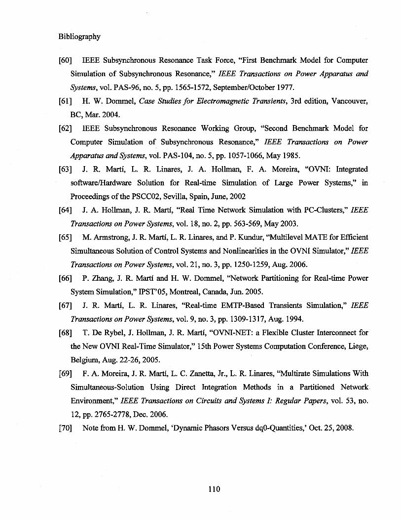
Bibliography
[60] IEEE Subsyncbronous Resonance Task Force, “First Benchmark Model for Computer
Simulation of Subsynchronous Resonance,” IEEE Transactions on Power Apparatus and
Systems, vol. PAS-96, no. 5, pp. 1565-1572, September/October 1977.
[611 H. W. Dommel, Case Studies for Electromagnetic Transients, 3rd edition, Vancouver,
BC, Mar. 2004.
[62] IEEE Subsynchronous Resonance Working Group, “Second Benchmark Model for
Computer Simulation of Subsynchronous Resonance,” IEEE Transactions on Power
Apparatus and Systems, vol. PAS-104, no. 5, pp. 1057-1066, May 1985.
[63] J. R. MartI, L. R. Linares, J. A. Hollman, F. A. Moreira, “OVNI: Integrated
software/Hardware Solution for Real-time Simulation of Large Power Systems,” in
Proceedings of the PSCCO2, Sevilla, Spain, June, 2002
[64] J. A. Hollman, J. R. MartI, “Real Time Network Simulation with PC-Clusters,” IEEE
Transactions on Power Systems, vol. 18, no. 2, pp. 563-569, May 2003.
[65] M. Armstrong, J. R. MartI, L. R. Linares, and P. Kundur, “Multilevel MATE for Efficient
Simultaneous Solution of Control Systems and Nonlinearities in the OVNI Simulator,” IEEE
Transactions on Power Systems, vol. 21,110. 3, pp. 1250-1259, Aug. 2006.
[66] P. Zhang, J. R. MartI and H. W. Dommel, “Network Partitioning for Real-time Power
System Simulation,” IPST’05, Montreal, Canada, Jun. 2005.
[67] J. R. MartI, L. R. Linares, “Real-time EMTP-Based Transients Simulation,” IEEE
Transactions on Power Systems, vol. 9, no. 3, pp. 1309-13 17, Aug. 1994.
[68] T. De Rybel, J. Hoilman, J. R. MartI, “OVNI-NET: a Flexible Cluster Interconnect for
the New OVNI Real-Time Simulator,” 15th Power Systems Computation Conference, Liege,
Belgium, Aug. 22-26, 2005.
[69] F. A. Moreira, J. R. MartI, L. C. Zanetta, Jr., L. R. Linares, “Multirate Simulations With
Simultaneous-Solution Using Direct Integration Methods in a Partitioned Network
Environment,” IEEE Transactions on Circuits and Systems I: Regular Papers, vol. 53, no.
12, pp. 2765-2778, Dec. 2006.
[70] Note from H. W. Dommel, ‘Dynamic Phasors Versus dqo-Quantities,’ Oct. 25, 2008.
110

Appendix A Machine Parameters
Appendix A
Machine Parameters
A.1 Synchronous Machine Parameters
TABLE A-ISmcHRoNous MACHINE PARAM1TERs
Parameters Hydro Turbine Generator Steam Turbine Generator
r3 0.00234 2 0.00243 2X, 0.1478(2 0.1538(2X 0.5911(2 1.457(2Xd 1.0467(2 1.457(2rfd 0.0005 (2 0.00075 (2X 0.2523(2 0.1145(2r1 - 0.00144(2Xlkql - 0.6578 (2r12 0.01675 (2 0.0068 1 (2X1 0.1267(2 0.07602(2rij 0.01736(2 0.0108(2X1 0.1970(2 0.06577(2J 3.51x10⁷Js2 6.58x10⁴Ps2Rating 325 MVA 835 MVALine-to-line
20 KV 26 KVvoltagePoles 64 2
111
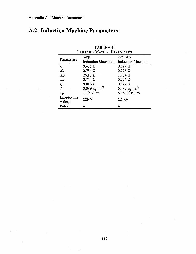
Appendix A Machine Parameters
A.2 Induction Machine Parameters
TABLE A-IlINDUCTION MACHINE PARAMi’rERs
3-hpInduction Machine0.435 20.754 2
2250-hpInduction Machine0.02920.2262
Parameters
rx’sXM 26.132 13.04Xir 0.754 2 0.226rr 0.816Q 0.022QJ 0.089kgm2 63.87 kgm2TB 11.9Nm 8.9x10³NmLine-to-line
220 V 2.3 kVvoltagePoles 4 4
112

Appendix B Voltage behind Reactance Induction Machine Model
Appendix B
Voltage behind Reactance Induction
Machine Model
This appendix faithfully reproduces reference [53], a project report for UBC course
EECE 549. The only difference here is that all equation numbers and figure numbers are added
with a ‘B.’. This report implemented the Voltage behind Reactance (VBR) model for the
symmetrical induction machine simulations. The discrete-time VBR model has the similar form
as the EMTP-type equivalent circuits. The simulation results validate the accuracy and efficiency
of this new induction machine model.
B. 1 Voltage Behind Reactance Model of Induction Machine
The equations of the induction machine can be expressed in the arbitrary reference frame
as
Vqs rslqs + + P)Lq (B.1)
VdS 1ds CO)Lqs +pAd$ (B.2)
= + pA0, (B.3)
o = rriqr + (o—
OJr )adr + Pqr (B.4)
o = rridr ( —0)r )Aqr + P21dr (B.5)
o = rrior + pA,0,. (B.6)
where each variable and parameter have been converted.to stator side, and
co = 0 for stationary reference frame, co = co,. for rotor reference frame and co = coe for
113
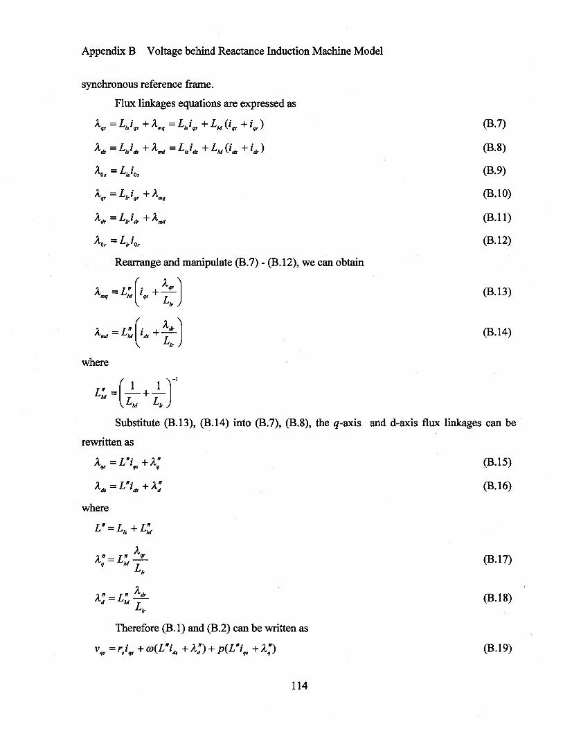
Appendix B Voltage behind Reactance Induction Machine Model
synchronous reference frame.
Flux linkages equations are expressed as
= Lislqs + Amq = Lis ‘qs + LM (‘qs + qr) (B.7)
= L1SIdS + Ad = L,SidS + LM (‘di + ld) (B.8)
A05 = L,5i05 (B.9)
Aqr LirIqr + Amq (B. 10)
Adr = Lirl& + A (B. 11)
‘0r =L1i0 (B.12)
Rearrange and manipulate (B.7) - (B.12), we can obtain
A,q = L [qs + (B. 13)
Amd1M[1ds +.z’,J (B.14)
where
LL =(+J’Substitute (B.13), (B.14) into (B.7), (B.8), the q-axis and d-axis flux linkages can be
rewritten as
Aq5 = L”1q5 + (B. 15)
A =L”idS +A’ (B.16)
where
L”—L -‘-L”— is M
(B.17)
(B.18)
Therefore (B.1) and (B.2) can be written as
Vqs = + o(L”idS + A) + P(1”lqs + A:) (B.19)
114

Appendix B Voltage behind Reactance Induction Machine Model
= rSidS — (D(L”qs + + p(L”i + (B.20)
By manipulating (B.1)-(B.18), we can obtain
=LZIqs )—(Co _Cor)2] (B.21)
1=r[
+LZidS _ar)+(0_C0r)2qr] (B.22)
Substitute (B.21), (B.22) into (B.19), (B.20), the voltage behind reactance form of the
voltage equations can be expressed
Vq = rsiqs + OJL”idS + P(L”lqs) + (B.23)
VdS = rSidS — (DL”lqs + P(L”lqs) + v (B.24)
where
=+ ‘‘
— lqg — —(co—
(B.25)
v=—coA:+(;—Adr)+i+(co—cor), (B.26)
Applying the inverse transformation to (B.23), (B.24), we can get the phase domain
equations
V (t) = (t) + p[L”i, (t)] + v(t) (B.27)
where
v(t) = [K(o)]’ v
0
L”L +±L” _LIs3M 3 3
LbCS = ——- L1+—L
L,+LZ
115
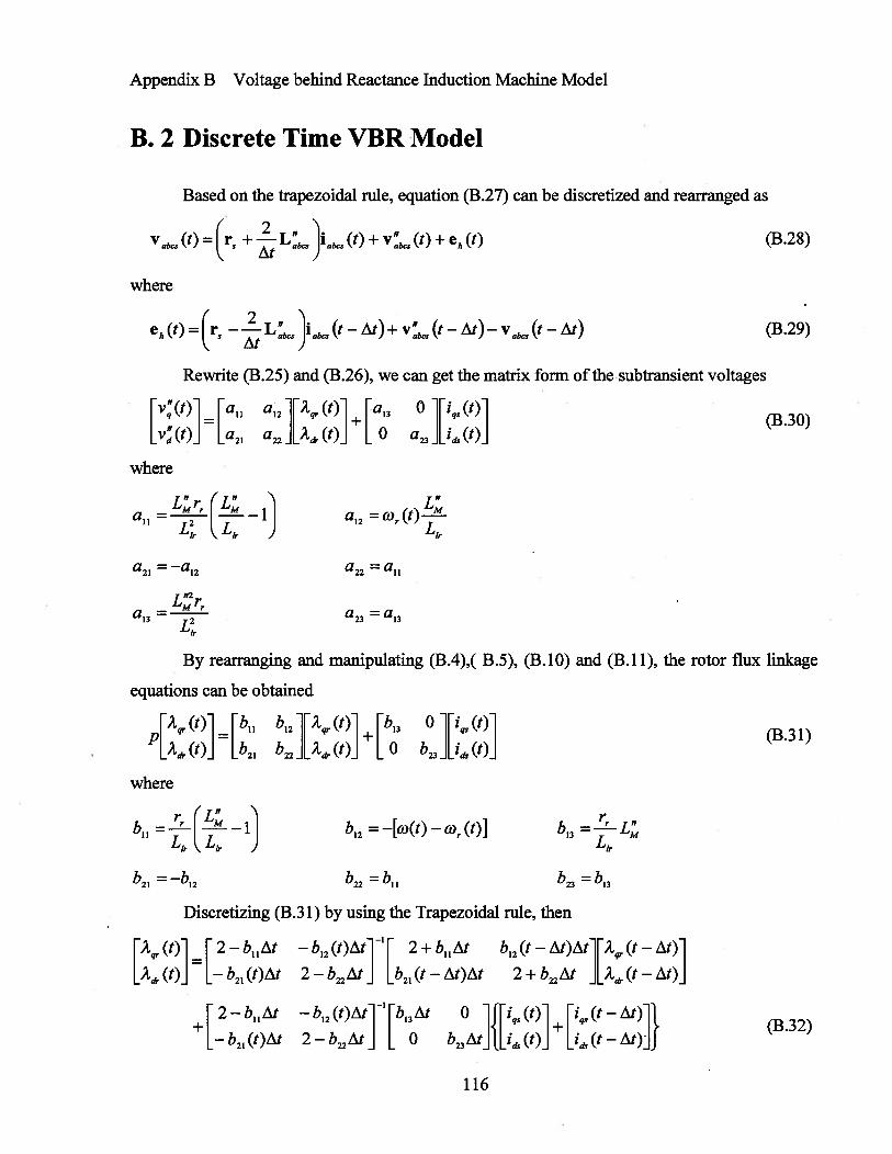
Based on the trapezoidal rule, equation (B.27) can be discretized and rearranged as
‘7abcs (t) = + --L5)iabcs(t) + vbC$(t) + ek (t) (B.28)
Ch (t) = — L5} abcs (t — At) + VbCS (t — At) — Vabcs (t — At) (B.29)
Rewrite (B.25) and (B.26), we can get the matrix form ofthesubtransient voltages
= fa11 a12 (t)1 + Ea130 ji (t)1 (B.30)
[v (t)J [a21 a22 ]Ldr (t)] [ 0 a3 ][i (t)]
a12 =Wr(t)jj
a22 = a11
a23 = a13
manipulating (B.4),( B.5), (B.10) and (B.11), the rotor flux linkage
(B.31)
Appendix B Voltage behind Reactance Induction Machine Model
B. 2 Discrete Time VBR Model
where
where
a =‘‘I—iL LL1r
a21 = a12
aLrr
13 L
By rearranging and
equations can be obtained
pH (t) E11 b12 (t)1 + rb!3 0 jIqs (t)
[A (t)J [b21 b22 ][A.. (t)] [0 b23 ][i (t)
where
b =--1-—1‘ L1L1,
b21 = —b12 b22 = b11
Discretizing (B.3 1) by using the Trapezoidal rule, then
E °‘)1 r 2 —b11At — b12 (t)At1 2 +b11At b12 (t — At)At1E (t — At)
L’dr (t)J [— b21 (t)At 2 —b22At J [b2, (t — At)At 2 +b22At J[2ar (t — At)
+2 —b11At — b12 (t)At1’ Ebi3At 0 Jj••1qS (t)1 + 1q5 (t — At)
2 — b22 At] [ 0 b23At] (t)J [i (t — At)
116
b12 = —[a(t) — 0)r (t)] b13 =--LZ
b23 = b13
(B.32)

Appendix B Voltage behind Reactance Induction Machine Model
Substitute (B.32) into (B.30), we can get the discrete time equations
r1 (i’)1
[ j =K(t)[ j+K2(t)vd(t) ldS(t)
where
K (t) = Hii a12 2—b11At — b12 (t)Atl1Ebi3At 0 1 + E’u13
[a21 a22 J[— b2 (t)At 2 —b22At] L 0 b23 At] [ 0 a23
K (t)— raii a12 ir 2 —b11At — b12 (t)Atlr 2 +b11At b12 (t
— At)&1r (t —
2— [ a22 ]L b21 (t)At 2 —b22At J[b2,(t — At)At 2 +b22At JL’dr (t — At)
+ Eaii a12 j 2 — b,1At — b,2 (t)At1’ P13 At 0 jqs 0’ — At)
[a2, a22 ][— b21 (t)At 2 —b22At] [ 0 b23At][idS (t — At)
Applying the inverse transformation to (B.33), we can transfer the qd0 variables to the
phase domain
VbCS (t) = K (t)Iabcs (t) + ChS (t) (B.34)
where
[K (t) 01K(t) = [K5 (0(t))]-’ [ j[K. (0(t))]
,EK 0’)ehS(t)=[KS(0(t))] LFinally, by substituting (B.34) into (B.28), the equivalent circuit for the stator voltage
equations can be written as
‘abcs (t) = G eqVabcs (t) — h(t) (B.35)
where
Geq [r5 + + K(t)]
h(t) =Geq[Ch(t) + ehS(t)]
117

Appendix B Voltage behind Reactance Induction Machine Model
B. 3 Free Acceleration Simulation of a 3-hp Induction
Machine
The first test case is to simulate the start-up transients of a 3-hp induction machine. The
parameters of the machine are
P=4 V1 220V r 0.4352 X, 0.754 2 XM= 26.13 2 X1r O.754
rr = 0.816c2 J 0.089 kg.m2.
The simulation results viewed from different reference frames are shown in Fig. B. 1- B.3.
(1) Figure B.1: Stationary Reference Frame
Because the initially position of the stationary qd0 reference frame is zero, thef = fqs.
Therefore the Iqs and Vqs are the same as i and v, respectively. The rotor variables are varying
at 60 HZ after referred to the stationary reference frame.
(2) Figure B.2: Rotor Reference Frame
At the very beginning, when the speed of the machine is slow, the variables in the rotor
reference frame are similar to those in the stationary reference frame. Then the stator variables
will vary at slip frequency when the rotor speed is increasing. After the speed reach the
synchronous speed, all variables in rotor reference frames becomes constant.
(3) Figure B.3: Synchronous Reference Frame
At stall the variables in the synchronous reference are varying at 60 HZ. The stator and
rotor variables will become constant when the rotor speed reaches synchronous speed. Note that
the zero position of synchronous reference frame that we chose is zero, therefore the magnitude
of Vqs is identical to this ofv and Vds is zero.
B. 4 Dynamic Performance of Induction Machine during
Mechanical Torque Changes
In this case, the machine originally operates in the steady state. At t = 0.05s, a constant
mechanical torque of 12 N.m2 is applied. Then the mechanical torque is reversed to -12N.m2at t
= 0.5s. The simulation time is ls.
Figure B.4 illustrates the simulation results with the VBR model.
118

Appendix B Voltage behind Reactance Induction Machine Model
0’
V
200.0
E 100
00
>0•
S0
0S
-100
0 0.1 0.2 0.3 0.4 0.5 0.6 0.7 0.8 0.9
Figure B.1 Free Acceleration Characteristics in Stationary Reference Frame
119
0.1 0.2 0.3 0.4 0.5 0.6 0.7 0.8 0.9 1
0 0.1 0.2 0.3 0.4 0.5 0.6 0.7 0.8 0.9

Appendix B Voltage behind Reactance Induction Machine Model
I i.J.. I
.:
0 06 07 08 09
1 OC
- I
0 0.1 0.2 0.3 0.4 0.5 0.6 0.7 0.8 0.9
30C I
\\45
0.6 0.7 0.8 0.9
,nn
______________________________________________________
I I I
2O0OjOi2Oi304 05 06 07 08 09
Figure B.2 Free Acceleration Characteristics in Rotor Reference Frame
120

Appendix B Voltage behind Reactance Induction Machine Model
I I I I I I I
0 0.1 0.2 0.3 0.4 0.5 0.6 0.7 0.8 0.9
2C I
C’
-4C I I I I I I I
0 0.1 0.2 0.3 0.4 0.5 0.6 0.7 0.8 0.9
-I (VI
JI0
0.1 0.2 0.3 0.4 0.5 0.6 0.7 0.8 0.9
50
0
-50
100
> -20
0.1 0.2 0.3 0.4 0.5 0.6 0.7 0.8 0.9
05 06 07 08 09
100O1
0I2 0I3 0I4 0i5 08 0I7 0809
300 I I I I I I I I I
Figure B.3 Free Acceleration Characteristics in Synchronous Reference Frame
121

Appendix B Voltage behind Reactance Induction Machine Model
21 22
22.12.2
2.3 2.4 2.5 2.6 2.7 2.8 2.9 3
j
500C
-500CI I I I I I
2 2.1 2.2 2.3 2.4 2.5 2.6 2.7 2.8 2.9 3
220C I I
iGoc
500C
—---
— I I I I I I I
2 2.1 2.2 2.3 2.4 2.5 2.6 2.7 2.8 2.9
Figure BA Dynamic Performance of a 3-hps Induction Machine during Step Changes in Load Torque
122

Appendix C Test Case Data
Appendix C
Test Case Data
%*********** ************ *** *** ********** ************ ******** ***************
% Test Case 1
% AnElectromagnetic Transient Program with Dynamic Phasor Solution
%
%
%
%
%
%
nBus=2;
Version 1.0 =
= Last revised: 24 Feb.2007 =
Peng Zhang =
= Copyright 2008 © Peng Zhang =
% P1 Line data
nLine=1; % Three phase line
LineFromBus(1)=1;
LineToBus(1)2;
I Ri ohm I Xl ohm I Cl muF 1R21 X2lC2l....
LineParameters =[0.0868455 0.0298305 0.0288883 0.2025449 0.0847210 0.0719161 0.00274 -0.0007 -0.00034;
0.0298305 0.0887966 0.0298305 0.0847210 0.1961452 0.0847210 -0.0007 0.00296 -0.00071
0.0288883 0.0298305 0.0868455 0.0719161 0.0847210 0.2025449 -0.00034 -0.00071 0.00274 1*10.56
% Load data
nLoadl;% Three phase load
LoadBus(1)=1;
rLoad(1,1)=(12.47*1000/sqrt(3))P2/(2000*1000); % phase A resistance
xLoad(1,1)=(12.47*1000/sqrt(3))t’2/(0.328684105 17886306346562595373367*2000*1000); % phase A reactance
rLoad(1,2)=(12.47*1000/sqrt(3)y2/(2000* 1000); % phase B resistance
xLoad(1,2)=(12.47*1000/sqrt(3)y2/(0.32868410517886306346562595373367*2000*1000); % phase B reactance
rLoad(1,3)(12.47*1000/sqrt(3))t2/(2000*1000);% phase C resistance
xLoad(1,3)(12.47* 1000/sqrt(3)y2/(0.32868410517886306346562595373367*2000*1000);% phase C reactance
% Voltage source data
nVSourcel;
VSourceBus(1)2;
Vabcs(1,1) 10182;%Vamp
Vabcs(1,2) = 10182 * exp(-jay * 2 * p / 3);
123

Appendix C Test Case Data
Vabcs(1,3) 10182 * exp(jay* 2 * pi/3);
T10= 3;
LineTripped = 1;
return;
%**************************************************************************
% Test Case 2
% An Electromagnetic Transient Program with Dynamic Phasor Solution
%
%
%
%
%
%
nBusl2;
Version 1.0 =
= Last revised: 24 Feb.2007 =
Peng Zhang =
= Copyright 2008 © Peng Zhang =
simT = 8; % total simulation time
ja’sqrt(-l);
ws2*pi*60;
% PT Line data
nLine=1 1; % Three phase line
LineFromBus(l)12;
LineToBus(1)=1;
LineFromBus(2)1;
LineToBus(2)4;
LineFromBus(3)4;
LineToBus(3)5;
LineFromBus(4)=1;
LineToBus(4)=2;
LineFromBus(5)2;
LineToBus(5)=3;
LineFromBus(6)=l;
LineToBus(6)6;
LineFromBus(7)6;
LineToBus(7)8;
LineFromBus(8)8;
LineToBus(8)9;
LineFromBus(9)8;
LineToBus(9)l0;
LineFromBus(10)=6;
LineToBus(10)1 1;
LineFromBus(1 1)6;
124
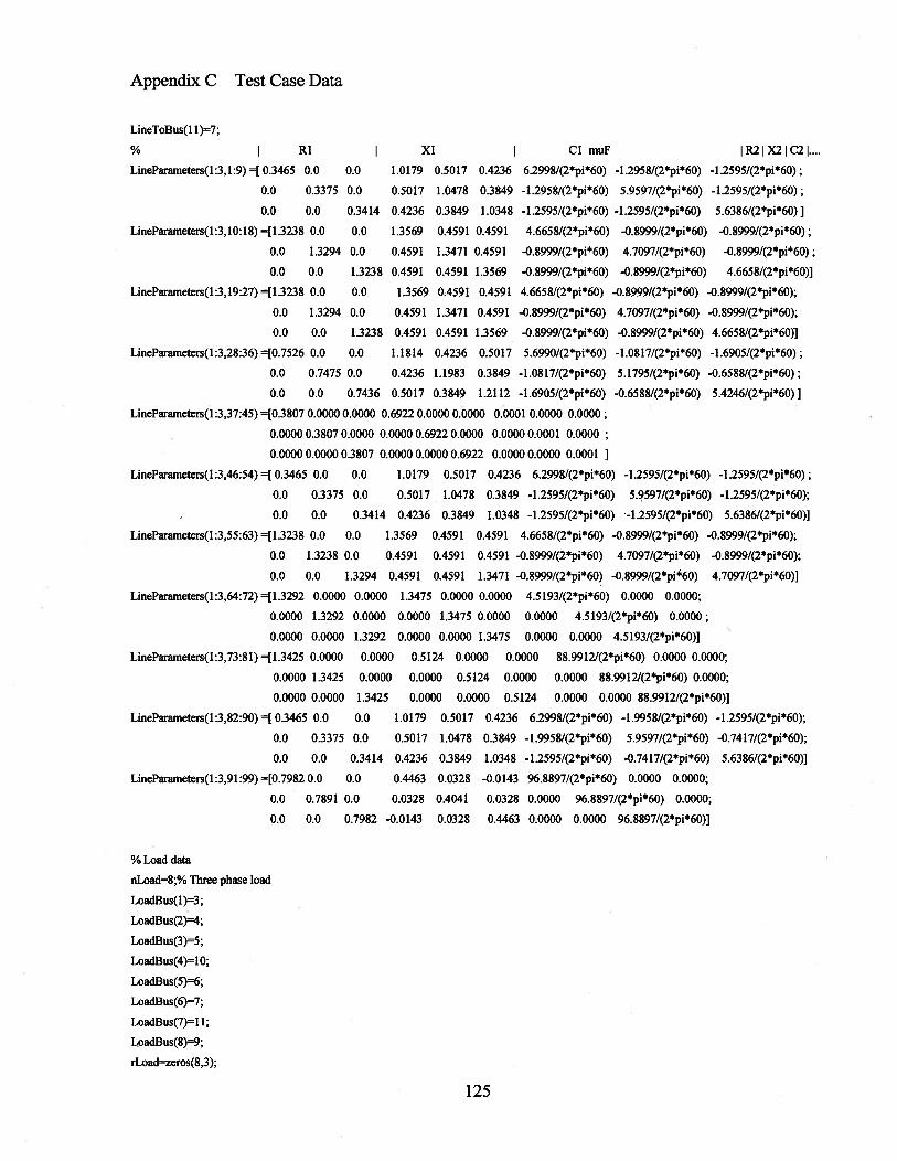
Appendix C Test Case Data
LineToBus(1 1)7;
I Ri I Xl I ClmuF 1R21X21C21....LineParameters(1:3,1:9)=[0.3465 0.0 0.0 1.0179 0.5017 0.4236 6.2998/(2*pi*60) _1.2958/(2*pi*60) 1.2595/(2*pi*60);
0.0 0.3375 0.0 0.5017 1.0478 0.3849 1.2958/(2*pi*60) 5.9597/(2*pi*60) 1.2595/(2*pi*60);
0.0 0.0 0.3414 0.4236 0.3849 1.0348 1.2595/(2*pi*60) 1.2595/(2*pi*60) 5.6386/(2*pi*60)]
LineParameters(1:3,10:18) =[1.3238 0.0 0.0 1.3569 0.4591 0.4591 4.6658/(2*pi*60) 0.8999/(2*pi*60) 0.8999I(2*pi*60);
0.0 1.3294 0.0 0.4591 1.3471 0.4591 0.8999/(2*pi*60) 4.7097/(2*pi*60) 0.8999/(2*pi*60);
0.0 0.0 1.3238 0.4591 0.4591 1.3569 .0.8999/(2*pi*60) .0.8999/(2*pi*60) 4.6658/(2*pi*60)]
LineParameters(1:3,19:27) =[1.3238 0.0 0.0 1.3569 0.4591 0.4591 4.66581(2*pi*60) 0.8999/(2*pi*60) 0.8999/(2*pi*60);
0.0 1.3294 0.0 0.4591 1.3471 0.4591 0.8999/(2*pi*60) 4.7097/(2*pi*60) 0.8999/(2*pi*60);
0.0 0.0 1.3238 0.4591 0.4591 1.3569 0.8999/(2*pi*60) 0.8999I(2*pi*60) 4.6658/(2*pi*60)]
LineParameters(1:3,28:36) [0.7526 0.0 0.0 1.1814 0.4236 0.5017 5.6990/(2*pi*60) 1.0817/(2*pi*60) 1.6905/(2*pi*60);
0.0 0.7475 0.0 0.4236 1.1983 0.3849 1.0817/(2*pi*60) 5.1795/(2*pi*60) 0.6588/(2*pi*60);
0.0 0.0 0.7436 0.5017 0.3849 1.2112 1.6905I(2*pi*60) 0.6588/(2*pi*60) 5.4246/(2*pi*60)]
LineParameters(1:3,37:45) =[O.3807 0.0000 0.0000 0.6922 0.0000 0.0000 0.0001 0.0000 0.0000;
0.0000 0.3807 0.0000 0.0000 0.6922 0.0000 0.0000 0.000 1 0.0000
0.0000 0.0000 0.3807 0.0000 0.0000 0.6922 0.0000 0.0000 0.0001
LineParameters(1:3,46:54) [ 0.3465 0.0 0.0 1.0179 0.5017 0.4236 6.2998/(2*pi*60) 1.2595/(2*pi*60) 1.2595I(2*pi*60);
0.0 0.3375 0.0 0.5017 1.0478 0.3849 1.2595I(2*pi*60) 5.9597/(2*pi*60) 1.2595/(2*pi*60);
0.0 0.0 0.3414 0.4236 0.3849 1.0348 1.2595/(2*pi*60) 1.2595/(2*pi*60) 5.6386/(2*pi*60)]
LineParameters(1:3,55:63) =[1.3238 0.0 0.0 1.3569 0.4591 0.4591 4.6658/(2*pi*60) 0.8999/(2*pi*60) 0.8999/(2*pi*60);
0.0 1.3238 0.0 0.4591 0.4591 0.4591 0.8999/(2*pi*60) 4.70971(2*pi*60) 0.8999/(2*pi*60);
0.0 0.0 1.3294 0.4591 0.4591 1.3471 0.8999I(2*pi*60) 0.8999I(2*pi*60) 4.7097/(2*pi*60)]
LineParameters(1 :3,64:72) =[1.3292 0.0000 0.0000 1.3475 0.0000 0.0000 4.5 193/(2*pi*60) 0.0000 0.0000;
0.0000 1.3292 0.0000 0.0000 1.3475 0.0000 0.0000 4.5193/(2*pi*60) 0.0000;
0.0000 0.0000 1.3292 0.0000 0.0000 1.3475 0.0000 0.0000 4.5193/(2*pi*60)]\
LineParameters(1:3,73:81)=[1.3425 0.0000 0.0000 0.5124 0.0000 0.0000 88.9912/(2*pi*60) 0.0000 0.0000;
0.0000 1.3425 0.0000 0.0000 0.5124 0.0000 0.0000 88.9912/(2*pi*60) 0.0000;
0.0000 0.0000 1.3425 0.0000 0.0000 0.5124 0.0000 0.0000 88.9912/(2*pi*60)]
Lineparameters(1:3,82:90) =[ 0.3465 0.0 0.0 1.0179 0.5017 0.4236 6.2998/(2*pi*60) .1.9958/(2*pi*60) ..1.2595/(2*pi*60);
0.0 0.3375 0.0 0.5017 1.0478 0.3849 1.9958/(2*pi*60) 5.9597/(2*pi*60) 0.7417/(2*pi*60);
0.0 0.0 0.3414 0.4236 0.3849 1.0348 -1 .2595/(2*pi*60) .0.7417/(2*pi*60) 5.6386/(2*pi*60)]
LineParameters(1:3,91:99) =[0.7982 0.0 0.0 0.4463 0.0328 -0.0143 96.8897/(2*pi*60) 0.0000 0.0000;
0.0 0.7891 0.0 0.0328 0.4041 0.0328 0.0000 96.88971(2*pi*60) 0.0000;
0.0 0.0 0.7982 -0.0143 0.0328 0.4463 0.0000 0.0000 96.8897/(2*pi*60)]
% Load data
nLoad=8;% Three phase load
LoadBus(1)’3;
LoadBus(2)=4;
LoadBus(3)5;
LoadBus(4)=10;
LoadBus(5)6;
LoadBus(6)=7;
LoadBus(7)1 1;
LoadBus(8)=9;
rLoad—zeros(8,3);
125

Appendix C Test Case Data
rLoad(:,:)1e6;
xLoad=zeros(8,3);
xLoad(:,:)=1e6;
rLoad(5,1)=(4. 16* 1000/sqrt(3))s2/(385* 1000); % phase A resistance
xLoad(5,1)=(4. 16*1000/sqrt(3))2/(220* 1000); % phase A reactance
rLoad(5,2)=(4. 16* l000/sqrt(3))/s2/(385* 1000); % phase B resistance
xLoad(5,2)=(4.16*1000/sqrt(3))f2/(220*1000); % phase B reactance
rLoad(5,3)=(4.16* l000/sqrt(3))f2/(385* 1000); % phase C resistance
xLoad(5,3)=(4. 16*100O/sqrt(3))l2/(220*1000); % phase C reactance
% Induction machine data
IndMacBus=1 1;
Ttorq=3; % torque applied
I S I VI I P J rs I Lls I LM I iT I Llr
IndMacParameters = [500 /(1.341e-3) 4600 4 11.06 0.262*4 1 .206*4/ws 54.02*4/ws 0.187*4 1 .206*4Iws];
% Voltage source data
nVSourcel;
VSourceBus(1)=12;
Vabcs(1,1) = (4.16*1000/sqrt(3))*sqrt(2) ; % Vamp
Vabcs(1,2) = (4.16*l000Isqrt(3))*sqrt(2) * exp(-jay * 2 * pj / 3);
Vabcs(1,3) = (4.16*l000Isqrt(3))*sqrt(2) * exp(jay * 2 * pi /3);
return;
126