buet, dhaka, july 15-17, 2004pdf.usaid.gov/pdf_docs/pnadd525.pdf · buet, dhaka, july 15-17, 2004...

Short Term Training on

Reliability and Operational Aspects of a Regional Grid

BUET, Dhaka, July 15-17, 2004

Table of Contents Agenda Overview of power system operation Role of reliability concept in a power system Decision variables for the optimal reliability level of a utility Devices for controlling power system operation Role of SCADA in power system operation Load carrying capability of newly added generating unit/units: Reliability aspects Evaluation techniques of reliability level of a single area utility Unit commitment procedure in meeting the demand economically Optimal dispatch of generating units Evaluation techniques of reliability level of interconnected utilities Interfacing of functions related to economic operation of interconnected power systems Concept and assessment of system security Capacity savings through interconnection and optimal tie line capacities Multi area evaluation approach in a single area system with limited transmission capabilities Secure operation of interconnected utilities

System reliability level: Impacts of load management schemes and joint ownership of generation Tutorials on reliability aspects Tutorials on operational aspects List of participants

Short Term Training on

Reliability and Operational Aspects of a Regional Grid Council Building (1st Floor), BUET, Dhaka, July 15-17, 2004

Organized by EEE Dept., BUET Sponsored by USAID and Winrock International

July 15, 2004 Thursday

INAUGURAL SESSION

08:30 Registration of Participants 09:00 Arrival of Chief Guest 09:05 Recitation from the Holy Quran 09:10 Welcome address and course overview

09:15 Introduction by participants and expectations in the training

09:30 Address by the Head, EEE Department, BUET 09:40 Address by local representative of USAID 09:50 Address by Chief Guest 10:00 Vote of Thanks 10:05 Refreshment

LECTURE SESSION 11:00 Overview of power system operation 11:45 Role of reliability concept in a power system 12:30 Decision variables for the optimal reliability level of a utility 13:15 Lunch 14:15 Devices for controlling power system operation 15:00 Role of SCADA in power system operation 15:45 Tea

16:00 Load carrying capability of newly added generating unit/units :Reliability aspects

16:45 Evaluation techniques of reliability level of a single area utility

July 16, 2004 Friday

08:30 Unit commitment procedure in meeting the demand economically 09:15 Optimal dispatch of generating units 10:00 TR1 11:00 Tea 11:30 Evaluation techniques of reliability level of interconnected utilities

12:15 Lunch & Prayer 14:00 Interfacing of functions related to economic operation

of interconnected power systems 14:45 Concept and assessment of system security 15:30 Tea 15:45 TO1

19:45 Dinner

July 17, 2004 Saturday

08:30 Capacity savings through interconnection and optimal tie line capacities

09:15 Multi area evaluation approach in a single area system with limited transmission capabilities

10:00 Secure operation of interconnected utilities 10:45 Tea

11:15 System reliability level: Impacts of load management schemes and joint ownership of generation

12:00 Discussion on “Regional grid: prospects, constraints and potential steps towards its achievement”

12:30 Lunch 13:30 TR2 14:15 TO2

15:00 Training Evaluation 15:15 Certificate Awarding 15:30 Tea 15:45 Special session for potential trainers selected from the participants (for others Site Visit)

TR = Tutorial on Reliability TO =Tutorial on Operation

1

S. Shahnawaz Ahmed, PhDProfessor, Dept. of Elect.& Electronic Eng.

BUET, Dhaka

Overview of Power System Operation

SOU

TH

ASI

A R

EG

ION

AL

INIT

IAT

IVE

/EN

ER

GY

Reliability and Operational Aspects of a Regional Grid, July 15-17, 2004, Dhaka

• Telephone vs. Power* Dial-Busy tone- “Wait and Call back later”

is the normal reaction from customers* Switch on electrical appliance-No power

(“Busy” e.g. fault)- “why not power now” is the reaction from customers

2

• Targets of power system operation1. Demand (MW) satisfied economically2. Voltage maintained3. Frequency maintained

• How to achieve?

• “MW” can be generated at power stations and despatched/exported to a far point.

• Nominal frequency can be maintained if MW generation is matched with MW demand.

• Voltage maintenance requires local injection of positive/negative “MVAR” . Because MVAR lacks mobility i.e. can not be despatched/transmitted as good as “MW”.

3

• Daily operation cycle (00-24 hrs)*Forecast demand (-24 hrs)*Choose units (-24 hrs)*bring them on-line (00-24 hrs)*Allocate load / (every 5 minutes)

review allocation *Send signals to generation units (instantly)

• What happens if- a unit is lost?- a transmission line is lost?- the interconnector goes into outage?- Contracted import is not firm/can not be

exceeded but local demand escalates?

4

• Entails the following depending upon severity of the outage and its effects

-load shed-brownout -blackout

• What is the redress? -Operational planning• What is that?-Differs from design/pre-implementation

stage planning done years (i.e.3-30x107

seconds) ahead• When to do it?-in real-time (i.e. 100 to around 4x103 seconds

ahead)

5

• Theme of operational planning:

-Monitor

-Manipulate

-Maintain

• “Manipulation” requires:-Decision support analyses-Convey decisions (sending commands

through SCADA)-Devices for execution (SCADA interfaced

with those devices)

6

• The whole thing of operational planning is automated in what is known as “EMS” i.e. Energy Management System.

• Development of EMS application functions require an effort of 20 man-years.

Bibliography

The lectures on ‘operational aspects of a regional grid’ delivered in this short-term training will help one navigate the too vast and diverse literature on power system operation objectively. Some of the titles suggested for further reading are as follows.

1.A.J. Wood and B. F. Wollenberg : “Power Generation, Operation and Control”, John Wiley & Sons, USA, 1996.

7

2.Hadi Saadat: “Power System Analysis”, McGraw Hill, Singapore, 1999.

3.J. J. Grainger and W. D. Stevenson, Jr.: “Power System Analysis”, McGraw Hill, Singapore, 1994.

4. W.A.Elmore, “Pilot Protective Relaying”, ABB-Marcel Dekker Inc., 2000.

5. N.G.Hingorani, “Flexible ac transmission”, IEEE Spectrum, April 1993, pp.40-45.

6.S. Shahnawaz Ahmed, S.Bashar, A.K.Chatterjee, M.A.Salam and H.B.Ahmad, “Use of superconducting magnetic storage device in a power system to permit delayed tripping”, IEE (UK) Proceedings-Genr. Transm. Distrib., Vol.147, No.5, September 2000, pp.269-273.

8

7. S. Shahnawaz Ahmed, Mahes Rajaratnam, Hussein Ahmad and Abu Bakar Sidik : “Potential Benefits of Using Distributed Parameter Model for Transmission Lines in Power System Analysis”, IEEE (USA) Power Engineering Review, Vol. 22, No.10, October 2002, pp.53-56.

8. S. Shahnawaz Ahmed, Narayan Chandra Sarker, Azhar b. Khairuddin, Mohd Ruddinb. Abd Ghani and Hussein Ahmad: "A Scheme for Controlled Islanding to Prevent Subsequent Blackout", IEEE (USA) Transactions on Power Systems, Vol.18, No.1, February 2003, pp.136-143.

9

9. Azhar B. Khairuddin, S. ShahnawazAhmed, Wazir b. Mustafa, Abdullah Asuhaimi b. Mohd Zin, and Hussein Ahmad: “A Novel Method for ATC Computations in a Large-Scale Power System”, IEEE (USA) Transactions on Power Systems, Vol.19, No.2, May 2004, pp. 1150- 1158.

10. Md. Abdus Salam and S. ShahnawazAhmed: “A New Method for Screening the Contingencies before Dynamic Security Assessment of a Multimachine Power System”, accepted for publication in European Transactions on Electric Power (Germany) and to appear in its early 2005 issue

1


BUET, Dhaka

Devices for Controlling Power System Operation

SOU

TH

ASI

A R

EG

ION

AL

INIT

IAT

IVE

/EN

ER

GY


• What are the operands?

-Frequency

-Voltage

-Real and Reactive Power

2

• Device for frequency control: generator governor

-Desired frequency-Sensed frequency-Control signal-Amplify-Valve control

Fig. A typical governor

3

• Speed changer-Provides set point-Shifts droop characteristics upward or

downward to schedule any output level from the generator at nominal frequency i.e. supplements governor action by letting in more or less energy from prime-mover

Fig. Governor droop characteristics

4

• It is the speed changer servomotor that can be operated either locally or by sending “raise” or “lower” pulses through SCADA.

• AGC (Automatic Generation Control)-single area or isolated system -interconnected system

5

Fig. AGC for a single area or isolated power system

Fig. AGC for two interconnected power systems

6

• Devices for voltage control:

- AVR for control from generator side

- VAR compensation devices for control from buses

Fig.LFC and AVR for a genertor

7

Fig. Details of a typical AVR

• LFC and AVR dynamics are weakly coupled as excitation system time constant is much smaller than prime-mover time constant.

• Voltage and frequency can be controlled almost independently.

8

• VAR compensation devices for voltage control from buses :

-synchronous condensers-SVC (e.g. STATCON, FC-TCR, TSC) under

FACTS family-TCUL and magnitude regulating (in-phase

booster) transformers

Fig.An SVC device comprising TCR and TSC/TCS

9

A FC-TCR (fixed capacitor-thyristor controlled

reactor) device

A static condenser (STATCON)

10

STATCON with all 3 phases shown

A TCUL transformer

kV 3

132

kV 3

33

11

An in-phase booster transformer

`

n

V an

V bn

V cn

∆ V anV an + ∆ V an

• Real power (MW) control devices:-control of injections from generator using

governor-control of flows in lines using (i) phase

shifting (quadrature booster) transformer or (ii) FACTS devices (e.g.TCSC,TCPA,UPFC)

12

A phase shifting transformer(details shown for phase-a)

Van

b

∆V=V'bcV'an =Van +V'bc

a

c

Vbc

V'bn =Vbn +V'ca

V'cn =Vcn +V'ab

The underlying phasor diagram for the phase shifting

transformer

V an

V 'bc

V 'an

V cn

V bn

V bc

θ

13

Fig. A thyristor controlled series capacitor (TCSC)

A thyristor controlled phase angle regulator(TCPA)

14

Unified power flow controller (UPFC)

A UPFC with all 3 phases shown

15

• Reactive power (MVAR) control devices:- control of injections from generator using

AVR- Control of flows in lines using (i)

magnitude regulating transformers or (ii) UPFC

• In addition to bus voltage and line flow control, FACTS devices can also damp out unwanted oscillations and hence improve dynamic performance of today’s highly stressed power systems.

1


BUET, Dhaka

Role of SCADA in Power System Operation

SOU

TH

ASI

A R

EG

ION

AL

INIT

IAT

IVE

/EN

ER

GY


SCADA (Supervisory Control and Data Acquisition) Features

• RTUs• Data Acquisition and Command implementation• Electrical and non-electrical data• Transducer, CT, PT etc.• Modem, Com. Links, RCS• Optimization of communication channels• LAN connected servers in master station• Hierarchical control

2

Basic structure of SCADA

Various communication links used in SCADA

3

Combination of radial (star) and multi-point (party line) master-RTU network

A typical layout of SCADA control centre

4

Recent developments and issues in SCADA

• RTU vs. IED• Use of GPS• Need of Standard Protocol

Connection of relay and transducers which are interfaced with a RTU

5

Direct interfacing between power system and an IED

6

Basic model of EMS that integrates application functions and

SCADA

Application Functions of EMS

• Data base: on-line data, fixed data, output of other functions.

• State Estimator: systematically cleans up raw data.

• Load Forecasting: real- time projection (half-an-hour to 24 hours ahead) of demand.

• Security control:monitoring, analysis, enhancement.

7

• Unit Commitment: usually 24 hours ahead decision on generating units/plants to be kept on or off.

• Economic Dispatch: how to allocate the generation share among committed units most economically.

• AGC: takes into account frequency mismatch, ED decisions and power interchange under contract.

Hierarchical control of a large power system’s operation

8

An example how respective SCADA/EMS system can be used by independent power

systems to coordinate their operation in interconnected mode

• Individual system’s detailed data can not be made available to one another i.e. the interconnection is not under “power pool”mode.

• So, no “pool control centre” exists. But each system’s EMS operators can communicate (voice or computer message) with theneighbouring systems’ ones e.g. via WAN.

• The following steps can then be taken.-Each system runs an economic dispatch (ED)

calculations for its own system and demand without assuming any power interchange with neighbours.

-By communicating with each other, the systems with lower incremental cost (IC) and those with higher one can then be identified.

9

-Then each system will carry out a series ofEDs by increasing the demand in each step (if lower IC) i.e. assuming an export or decreasing the demand (MW) in each step (if higher IC) i.e. assuming an import, and determine respective IC in each step.

-In each step the systems will communicate among them only respective IC and demand increment or decrement size (MW).

- If in a certain step the ICs for all the systems are found to be almost equal, the level of interchange (export or import) by each system can be determined from increment or decrement in its demand corresponding to that step.

- This will lead to almost the same conclusions on cost and size of transactions if a pool dispatch were performed considering all the interconnected systems as a single area.

1


BUET, Dhaka

Unit Commitment Procedure in Meeting the Demand Economically

SOU

TH

ASI

A R

EG

ION

AL

INIT

IAT

IVE

/EN

ER

GY


What is unit commitment (UC)?

• A procedure based on a heuristic /rigorous /semi-rigorous / artificial intelligence method

- to decide usually 24 hours ahead- which ones of the available generation units

should be turned on or off , - when, - and how long- so that the total fuel cost for satisfying the

forecasted load profile for the next 24 hours can be minimized.

2

Why it is needed?

• A utility has many generation units from reliability as well as operational needs.

• These are of varying characteristics and operating costs.

• These are at various distances from load centres.• The daily demand profile is not static. • A reduction in fuel cost by even 0.5% in a day

represents a saving of millions of dollar over one year for a large utility.

Complexities

• A plethora of constraints• Generation mix i.e. hydro and thermal units• Scheduled interchanges with neighbouring

utilities through interconnections.• If K units then there are 2K –1 possible

combinations to be examined in each stage or interval (e.g. every hour) of the study period (e.g. 24 hours).

3

Some simplifications

• Make the most of available hydropower (that implies zero fuel cost) within the transmission line limits.

• Given the scheduled interchange, commit the thermal units.

• Fortunately, all of the 2K –1 combinations are not feasible and hence may be ruled out, thanks to many constraints including demand vs. capability.

What are the main constraints to be considered ?

• Spinning reserve• Minimum up time of units• Minimum down time of units• Start-up cost that varies with hours of

operation the unit was in.

4

• Units that must run during certain times of the year

• Limited fuel or obligation to burn a specified amount of fuel in a given time

• Variable capacity of units due to maintenance or unscheduled outages of their components

Methods for UC

• Choice of method is important as the conclusion (i.e. savings in fuel cost) varies from method to method.

• However, none of the methods will result in the true optimal solution while their individual accuracy vary. This is due to assumed simplifications and the way a method takes into account the constraints.

• The most accurate method is not necessarily the one that poses the least computational burden.

5

Widely used methods

• Priority listing• Lagrangian relaxation• Dynamic programming

Priority listing

• The simplest method in respect of computational requirements.

• The units are ranked in descending order of respective full load average fuel cost (a linear input-output characteristics is assumed throughout the operating range).

• Priority in committing the units starts with the lowest ranked one.

• Further enhancements can also be made to include other constraints.

6

Lagrangian relaxation

• This is somewhat rigorous mathematics based method.

• The UC problem is formulated as minimization of an objective function, that in its simplest form takes into account the fuel cost (Fi), start up cost (Si) , and on/off status (Ui = 1 or 0) of all the units K in each interval ‘t’ of the window (study) period.

• The minimization is done subject to only two constraints viz. loading constraints (i.e. demand equals total of all the committed generation units’outputs) and units’ capacity limits, in each interval.

• The Lagrange function isL =∑t=1 to N ∑i=1 to K[Fi(Pi

t,Uit) +Si,t] Ui

t

+ ∑t=1 to Nλt (Ptload - ∑i=1 to K Pi

tUit) (1)

7

• Then minimization is done in two steps (or dual optimization) in each interval t.

-Firstly a λ is obtained for which L (excluding Pt

load that is constant) is maximized.-Keeping this λ fixed, Pi

t and Uit are adjusted

so that L (excluding Ptload that is constant) is

minimum subject to the units’ capacity limits.

• Other constraints can also be included in the second step of dual optimization.

• Due to convergence problem, Lagrangian relaxation method is run in combination with dynamic programming method in few initial iterations and a heuristic method in the later iterations.

8

Dynamic programming (DP)

• This is a semi-rigorous method and computationally also efficient.

• The UC for the whole window (N intervals) is divided as a number of optimization subproblems, one for each interval t so that the combined best decision for N subproblems yield the overall solution for the original UC problem.

• This combined with consideration of practical constraints leads to a phenomenal reduction in the number of candidate combinations to be examined by DP.

9

• In DP, equation (2) is used iteratively starting with the final stage (interval) N and carrying the cumulative minimum cost for each of the feasible combinations in the stage (t+1) i.e. xi(t+1) backward in time to each feasible combination i in stage t so that the minimum cumulative cost Fi*(t) can be found for each xi(t) .

Fi*(t) = [min{fi(t) +Tij(t)+Fj(t+1)}j=1……xj(t+1)]i=1….xi(t)

(2)where,fi(t) = fuel cost in stage t for its i-th feasiblec

combinationTij(t) = cost of transition from combination xi(t) to

combination xj(t+1) due to start up or shut down of one or more units.

10

• In this way eqn. (2) is applied till the first stage is reached.

• The optimal unit commitment schedule from stages 1 to N is then found by tracing the path that joins that specific feasible combination in each stage at which the cumulative cost becomes minimum when compared with cumulative cost at other feasible combinations in the same stage.

An example on UC of a 4-generator system using DP

• In a power system the daily load cycle experiences 1100 MW, 1400 MW, 1600 MW, 1800 MW, 1400 MW and 1100 MW respectively for stages 1 to 6. Each stage consists of 4 hours as shown in Fig. 1.

• There are 4 thermal generation units in the system having loading limits and quadratic fuel-cost characteristics with coefficients given in the Table 1.

11

Fig.1: Daily load cycle

Table 1:Loading limits and cost coefficients of 4 generators

Unit Minimum Maximum a ($/h/MW2) b ($/h/MW) c ($/MW)loading loading

1 100 MW 625 MW 0.0080 8.0 500

2 100 MW 625 MW 0.0096 6.4 400

3 75 MW 600 MW 0.0100 7.9 600

4 75 MW 500 MW 0.0110 7.5 400

12

• Let us consider that units 1 and 2 be treated as the must-run units.

• Assume that the start-up and the shut-down costs for each unit are $3000 and $1500 respectively.

• Consider that only the must-run units 1 and 2 will run in the 1st and the last (i.e.6th) stages of load cycle.

• Neglect transmission losses.• Use the dynamic programming approach

and determine the optimal unit commitment schedule for the system.

13

Solution

• First of all, for every stage (t) make an economic dispatch (ED) i.e. find the allocation of generation output for the units in each feasible combinations (within the constraints imposed) xi(t) and also the corresponding fuel or production cost fi(t).

• This is shown in Table 2. The way the ED has been done will be illustrated in an example in the next presentation on “Optimal dispatch of generating units”.

Table 2: ED results for feasible combinations

Comb.code Outputs in MW Total fuel cost/stage P1 P2 P3 P4 $

Stage 1,6Pload=1100 MWx1 (1111) 261 385 219 235 45,848x2 (1110 ) 351 459 290 - 45,848x3 (1101 ) 347 456 - 298 44,792x9 (1100) 509 591 - - 45,868

Stage 2,5Pload=1400 MWx1 (1111) 351 459 290 300 58,428x2 (1110 ) 464 554 382 - 59,356x3 (1101 ) 464 553 - 383 58,236x9 (1100) Infeasible

14

Table 2 /contd.Comb.code Outputs in MW Total fuel cost/stage P1 P2 P3 P4 $

Stage 3Pload=1600 MWx1 (1111) 410 508 338 344 70,908x2 (1110 ) 541 617 442 - 68,976x3 (1101 ) 542 618 - 440 67,856x9 (1100) Infeasible

Stage 4Pload=1800 MWx1 (1111) 469 558 386 387 76,472x2 (1110 ) 625 625 550 - 79,184x3 (1101 ) Infeasiblex9 (1100) Infeasible

Stage 6

• Now, begin with last stage (N=6). Though there are 4 feasible combinations. But it has been restricted that only the combination x9with only units 1 and 2 in ON state is to be considered.

• Apply equation (2) to this stage with only one i.e. x9 combination as the candidate.

• Since this is the last stage, cumulative cost Fj(t+1) up to this stage is zero.

15

• Since the first and the last stages are same in respect of demand and commitment (i.e. x9), the transition cost Tij(6) becomes zero.

• Now, on substituting f9(6) = $45,868 (for x9) the minimum production cost at stage 6 i.e. F9(6) becomes the same.

Stage 5

• Here feasible combinations are xi(5) = x1(5), x2(5), x3(5)

• In stage 6 the feasible combination was only one i.e. x9

• So eqn. 2 is to be applied by permutation of x1(5), x2(5), x3(5) each with x9(6).

16

• As for example,F1(5) = {f1(5)+T1,9(5)+F9(6)}=

{$58,428+$3000+$45,868}= $107,296Similarly, F2(5) = $106,724F3(5) = $105,604

Stage 4

• For this stage more permutations need to be done as there are 3 feasible combinations in stage 5 and 2 feasible combinations in stage 4.

• Applying eqn. (2) for each of x1 and x2 with 3 cumulative costs from stage 5 i.e. F1(5), F2(5) and F3(5) we can have minimum F1(4) and F2(4).

• All the cumulative costs in each stage and for each feasible combination are recorded in Fig.2.

17

Stage 3, 2, 1

• Eqn. (2) is applied for each of the stages in the way it was done for stage 4.

• Then it can be found that at stage 1for the lone combination x9(1) the cumulative cost function that was being carried back from stage 6 will stand at $361,536.

Fig.2: DP solution for the example UC problem

18

Optimal UC schedule for this example

• If the least cumulative cost path is traced from stage 1 to 6 then it is found that x9 in stage 1 derives from combination x3 in stage 2, which in turn derives from x3 in stage 3, and so on back to x9 in stage 6. This is summarized in Table 3.

Table 3: UC schedule for the example case

Stage load level comb. Units on/ofin MW

1 1100 x9 11002 1400 x3 11013 1600 x3 11014 1800 x1 11115 1400 x3 11016 1100 x9 1100

19

• In the example case, the total fuel cost to supply the forecasted load for 24 hours is $361,536.

A note

• The UC problem as discussed here can also be extended for a utility that has scheduled imports through interconnections with neighbours or power purchase agreements with IPPs.

• This can be done by treating the “import” / “agreed purchases” as equivalent must-run unit capacity in the corresponding intervals (stages).

1


BUET, Dhaka

Optimal Dispatch of Generating UnitsSO

UT

H A

SIA

RE

GIO

NA

L IN

ITIA

TIV

E/E

NE

RG

Y


• What is this?- This is popularly also known as economic

dispatch (ED). - This is a computational procedure by which the

generation is allocated among the units that have already been brought on-line i.e. committed in an interval of time (stage) such that the production cost in that stage is the optimum i.e.minimum subject to some constraints such as demand and transmission losses.

2

• How does it relate to UC?- Indeed, UC also requires that an ED be performed

in each stage. However, that is done for each of many feasible combinations not a specific one and yet to be implemented.

- Furthermore, ED when done as a part of UC it allocates generation outputs among the candidate units to meet a forecasted load, and usually does not consider even line losses.

ED for generators within a plant

• Transmission losses do not arise in this case.

• If the generators are loaded at such values that their respective incremental costs (λi)are equal to each other and the demand (PD) is equal to sum (PT) of their outputs, then this will result in an ED.

3

• The incremental cost λi of a generator (i-thunit) at its any output Pi is the additional cost per hour to increase the output by 1 MW i.e. Pi +1 MW.

• This is variable and depends on the fuel characteristics (input-output curve) i.e. MBtu/h vs. MW curve for a thermal unit.

• λi = dfi/dPi (1)

• The fuel cost in $/h is obtained by multiplying the fuel input by the cost of fuel in $/MBtu.

• Typically the fuel cost curves are quadratic and very often approximated in terms of vendor supplied coefficients as follows.

• fi = (ai/2)Pi2 + biPi + ci $/h (2)

4

• λi = dfi/dPi = aiPi + bi $/MWh (3) • For ED,λi = λ = aTPT + bT; i=1,2…..K (total no.of

generators under ED) (4)λ is also termed plant λ.whereaT = {∑i=1 to K (1/ai)}-1 (5)bT = aT {∑i=1 to K (bi/ai)} (6)

PT = ∑i=1 to KPi = PD (7)

Individual economic (optimal) output is thenPi = (λ - bi)/ai (8)

5

An example of ED for a power plant

• Let the example given in UC be considered.• Let the ED be made for stage 1 with

combination x1 (all the units to be run) for aPD=1100 MW.

Table 1:Loading limits and cost coefficients of 4 generators

Unit Minimum Maximum a ($/h/MW2) b ($/h/MW) c ($/MW)loading loading

1 100 MW 625 MW 0.0080 8.0 500

2 100 MW 625 MW 0.0096 6.4 400

3 75 MW 600 MW 0.0100 7.9 600

4 75 MW 500 MW 0.0110 7.5 400

6

• Solution:• Using equations (5), (6) and a,b,c

coefficients of 4 generators from Table 1aT = 2.3805x10-3

bT = 7.4712• Using equation (4) and PT = PD =1100 MWλ = 10.090 $/MWh

• Using eqn. (8), λ, and a,b, c of each unit, the ED outputs are obtained as

P1 = 261 MWP2 = 385 MWP3 = 219 MWP4 = 235 MW

7

• Substituting the ED outputs in eqn. (2) respective fuel costs are obtained as

f1= 2861 $/hf2= 3565 $/hf3= 2570 $/hf4= 2466 $/h• Total generation cost in stage 1 that comprises 4

hours would be 4 times the sum of f1 to f4 i.e. $45,848

ED for a number of plants

• Each plant may be considered to have a lumped output Pi and a plant incremental cost λi.

• Transmission losses now must be considered as a cheaper plant with low incremental cost may be far from the load centre.

• If the plants are allocated outputs Pi such that the product of respective λi and penalty factor Li is equal to that of another plant then ED has been achieved.

8

• λi Li= λ; i=1,2…….No. of plants (9)λ is now termed ‘system λ’• It is the penalty factor that takes into account

transmission losses in ED among plants.Li= 1/(1-∂PL/ ∂Pi) (10)where PL is total transmission loss in the system PL = ∑i=1 to S ∑j=1 to S PiBijPj (11) • ∑i=1 to S Pi = PD+PL (12)

• Eqn. 11 is a typical equation that expresses transmission loss in terms of B coefficients for S No. of sources connected to the transmission network.

• The source No. S must also include the additional points of power import into the transmission network such as scheduled import through interconnections or from hydropower plants. Because these imports contribute to PL and hence affects distribution of remaining loads among the thermal plants.

9

• This means for a 5-thermal plant system with 3 hydro plants and 7 interconnections, the loss coefficient (B) matrix will be 15x15 though only 5 thermal plant outputs to be obtained through ED.

• Usually a number of B coefficients sets corresponding to typical parts of the daily load profile are obtained by a series of off-line load flow solutions, and used in different stages (intervals) for ED.

1


BUET, Dhaka

Interfacing of Functions Related to Economic Operation of Interconnected

Power Systems

SOU

TH

ASI

A R

EG

ION

AL

INIT

IAT

IVE

/EN

ER

GY


Application functions directly related to economic operation

• Unit Commitment(UC): usually 24 hours ahead decision on generating units/plants to be kept on or off.

• Economic Dispatch: how to allocate the generation share among committed units.

• AGC: attempts to remove frequency mismatch, implements ED decisions and power interchange under contract.

2

Fig.1 Underlying logic of an AGC schemein each of the interconnected areas (systems)

Fig. 2 Use of SCADA in generation control

3

Role of ACE (Area Control Error)

ACEi = ∑(Pit,actual - Pit,scheduled)t - Bi ∆f (1)

where t implies all the tie lines (interconnections) between the area ‘i’ and other areas.

• The ACE of each area is to be zero. • If there is a loss of generation or change in

demand the ACE of only that area increases to such a value that the remaining generators, committed on-line in that area, will be forced to increase generation.

• ACE concept is effective only if the changes are such that the systems remain in steady state.

4

Role of participation factor (pf)

• ACE in each area serves to indicate whether total generation in the area needs to be raised or lowered.

• Now, the problem is that once having decided the base point generation (Pibase) of each unit by an ED at a regular interval, how to reallocate among the units the change in total generation (∆Ptotal) before the next interval?

• The solution is a pre-calculated participation factor (pfi) for each unit so that

Pides = Pibase + pfi x ∆Ptotal (2)where,Pides = new desired output from unit i∆Ptotal = Pnew total - ∑Pibase (3)

5

• The AGC control logic is also driven by the unit errors i.e. deviations of each generation unit from the desired economic output Pides

• To do the above, the sum of the unit errors (also termed SCE) is added to the concerned area’s ACE to form a composite error signal that drives the entire control system. This is what shown in Fig.1 that combines UC-ED with AGC.

An example of Steady state operation of AGC for three systems that are

interconnected• Three interconnected 60 Hz control areas

with autonomous AGC systems have respectively the following aggregate speed-droop (R) characteristics, on-line generation capacities (S) and frequency bias settings (B). Each area has a zero frequency-sensitive load coefficient (D).

6

R (p.u.) S (MW) B (MW/Hz)Area A: 0.0200 16,000 -12,000 Area B: 0.0125 12,000 - 15,000 Area C: 0.0100 6,400 - 9,500

• Each area has a load level equal to 80% of its rated on-line capacity. For reasons of economy, area C is importing 500 MW of its load requirements from area B, and 100 MW of this interchange passes over the tie lines B-A-C. Area A has a zero scheduled interchange of its own. The scenario is as in Fig. 3.

7

Fig.3: Operation scenario in a 3-area interconnected system

• i)What is the system frequency deviation (in Hz) and the generation changes (in MW) in each area when a fully loaded 400-MW generator in area B goes into forced outage?

• ii)What is the ACE (in MW) of each area before AGC action begins following the loss of the 400-MW generator in area B. Neglect losses in each area?

8

∆f (i.e. change in frequency in Hz) = ∆P (i.e. load change in MW)/ SUM (4)

where, • ∆P is negative for addition in load or loss

of generation• ∆P is positive for loss of load or surplus of

generation

• SUM = ∑((1/R)+D)i ; i= 1....No. of areas.• Ri (in Hz/MW) = (Ri (in pu) x f0) / Si ( i.e.

Rated MW capacity as base)• ∆f (in pu) = ∆f (in Hz) /f0 (rated frequency)• Individual generation change (∆Pgi ) in each

area in response to load change is given as∆Pgi (in MW) = ∆f (in Hz) /Ri (in Hz/MW)

(5)

9

i) The loss of the 400 MW is sensed by other on-line generators as an increase in load leading to a decrease in frequency given below, as determined by eqn. (4).

∆f = - 0.01 Hz i.e. –10-3/6 pu on f0 = 60 Hz basis

ii)The decrease in frequency leads to initial governor action of each of the remaining on-line generators in each area and causes increments in their outputs given below, as determined by eqn. (5).

∆PgA = 133 MW∆PgB = 160 MW∆PgC = 107 MW

10

• The increments in generations of the 3 areas following a loss of generation in area B and before AGC acts, will cause a redistribution of flows over the interconnections as in Fig. 4.

Fig. 4: Scenario after loss of a generator in the exporting area B

11

The ACEs in each area is then given below as determined applying eqn. (1).

ACEA = 13 MW

ACEB = -390 MW

ACEA = 12 MW

Inferences:• The increments in all 3 areas’ generation is

for a momentary period only.• The ACE in area B where generation loss

occurred is very high, and will command though AGC action the remaining on-line generators in B to increase their generation to make ∆f = 0 for all the areas.

12

• Once the frequency is restored to original 6o Hz, the generations in other areas A and C where ACEs are significantly much low (ideally zero) will be restored to their original values.

• The unavoidable or inadvertent energy interchanges (accumulated over a period) due to tie line flows beyond contract for the momentary time can be paid back either in cash or in “energy for energy”, on terms mutually agreed upon by the interconnected utilities.

1


BUET, Dhaka

Concept and Assessment of System Security

SOU

TH

ASI

A R

EG

ION

AL

INIT

IAT

IVE

/EN

ER

GY


Economy vs. Security

• “Security” must prevail over “economy”• Considering mere the cost characteristics,

minimum up/down time etc. of plants and line losses in making UC (Unit Commitment) and ED (Economic Dispatch) may result in cost optimization (i.e. economy) but not in “secure operation” of an interconnected or any power system.

2

• Security refers to a mode of operating a system such that at any time if any component (e.g. line/transformer/generator) fails the system will not experience “cascaded outage” or blackout.

• The question is why should security get so much importance when the reliability aspect has been considered at the planning stage?

• The answer is “simple”. • Studies carried out at the planning stage

years or even days ahead with respect to certain conditions can not cater to all the loading situations, generating patterns and the wide range of outages (contingencies) likely to arise when the system actually operates.

3

• A hypothetical solution can be provision of “highly adequate” reserve margins in generation and transmission capacities at the planning stage.

• But as reserve margin represents a large investment in spare (standby and uncommitted i.e. not in operation) equipment, this has to be limited.

How will security affect economy?

• A good example is a simple system as in Fig. 1 in which a hydro plant (being cheap) is committed and allocated 500 MW to supply over a double circuit line to a load centre that has 1200 MW demand. Each circuit has a thermal loading capability of maximum 400 MW.

4

Fig.1: Economic dispatch in a power system

• The operating condition in Fig. 1 represents an optimal or economic dispatch (ED). If one circuit trips due to a fault, such an operation will evidently result in overloading of the remaining circuit by an extra 100 MW that may also eventually trip.

• So ED may lead to insecure operation if the contingencies and constraints (e.g. line loading limit) are not considered.

5

• A solution to an insecure ED for the system in Fig. 1 is that shown in Fig. 2 where the cheaper hydro is allocated 100 MW less. As a result in the event of a contingency like outage of one circuit, this operating condition will not lead to any collapse of the system. This is called “secure dispatch”.

Fig.2:Secure dispatch in a power system

6

• A comparison of Figs. 1 and 2 tells us : better loose some “profit” but don’t risk “blackout”.

• This is what security i.e. run the system thinking of contingencies ahead of their occurrences.

How to implement security?

• Indeed, many utilities are practicing security concept in a primitive way. Even this does not involve ICT (information & communication technology) gadgets and sophisticated “3M” method i.e. monitor-manipulate-maintain.

• Rather, a thumb rule “load each circuit of a line to a maximum of half its thermal loadability” (i.e. as in Fig. 2) is followed.

7

• Similarly, “commit sufficient generation to maintain enough spinning reserve to compensate against a loss of a generation unit” is another thumb rule.

• However, the primitive way is too conservative in today’s context and compromises economy too much.

• Furthermore, adjustments of generation throughout a large system to effect even the thumb rules is beyond the capability of operators not aided by SCADA system.

8

Problems in implementing security

• Large system size• ‘Infinite’ number of contingencies• Speed limitations of the analytical /heuristic

tools for analyzing the effects and taking measures against so many contingencies even on today’s fast processors.

Real-time compatible solution

• Monitor to classify the system operating condition into one of the 4 states viz. ‘normal’, ‘alert’, ‘emergency’ and ‘restorative’.

• Screen the contingencies• Security constrained optimization

9

Figure 3 Typical classification of power system security related states

What are the constraints?

• Basically three sets of constraints viz. operating, load and security constraints.

• The operating constraints comprise mainly the operational limits on system variables and apparatus, for instance voltage limit, generator loading limit, transmission line thermal limit, tap position limit and so on.

10

• The load constraints mainly refer to customers’ total power demand.

• The security constraints are mainly the minimum reserve margin in generation and transmission capacity that is committed (i.e. in operation). These are also termed respectively “spinning reserve” and “transmission margin”.

• A system is in the normal state when all the constraints are met such that the occurrence of any credible but unforeseen disturbance or contingency (e.g. loss of line /generator /transformer/load) will not lead the power system to the emergency state.

11

• In emergency state the operating and security constraints are violated and the load constraints are not necessarily satisfied. “Blackout” is an extreme version of emergency state.

• In alert state security constraints are violated.

• Notably, many utilities in South Asian countries lack in requisite spinning reserve and hence are always in alert state.

12

• A system in normal state can go to alert or emergency state when any of the security constraints are violated.

• If a sufficiently severe disturbance takes place before control action can be taken, the system in the alert state enters the emergency state or its extreme version i.e. blackout state.

• The restorative state is a “transit” state between the emergency or blackout state and the normal state.

• This is associated with the period in which actions (ranging from fast valving, dynamic braking, etc. to load shedding, islanding, resynchronization etc.) are taken to bring the system from the emergency/blackout back to the normal state.

13

Contingency screening

• Do not bother the myriads of contingencies rather identify / select only a few of them that pose potential threats i.e. critical cases. Such a screening technique may involve simple DC load flow or linear sensitivity factors to correlate the effects on system to the contingency e.g. outage of a generator or line. Fast decoupled AC load flow is also used occasionally.

Security constrained optimal power flow (SCOPF)

• Run an SCOPF i.e. make a series of ED for each of the selected contingencies subject to the load flow equations, constraints on line flow, bus voltage, tap change, spinning reserves etc.

14

Difference between ED, OPF and SCOPF

• Normal ED optimizes only fuel cost considering generation unit capacity related constraints, demand and line losses.

• OPF optimizes fuel cost or line losses subject to the load flow equations and operational constraints.

• SCOPF considers contingencies and security constraints in addition to what is considered in OPF.

Outcome of SCOPF

• This will lead to a preventive operating strategy for a system identified to be in alert state.

• The preventive measures comprise any or all of the means such as redispatch of generation, VAR injections, shifting line flows or switching lines, transformer tap adjustments, and rescheduling (there must be provision for this in the contract) interchanges with neighbours so that the security constraints are not violated in the event of actual occurrence of any contingency.

15

Steady state and dynamic security

• Let’s refer back to Figs. 1 and 2.-When a circuit would go into forced outage

(i.e. a major disturbance), it was shown that the system would still operate with the other circuit exceeding (Fig. 1) or remaining within (Fig. 2) its normal loading limit.

-But the possibility that such a major disturbance can lead to loss of synchronism i.e. transient stability of the generators, has been overlooked.

-ORIt has been assumed that the generators’

swings subsided (transient stability maintained) and the system has gone to steady state.

16

• So if contingency screening is done with the assumption of “regaining steady state condition following a contingency”, it is termed steady state security assessment.

• On the contrary, if contingency screening takes into account the transient stability aspect following a contingency, it is termed dynamic security assessment.

• Usually screening the contingencies for dynamic security assessment involves various analytical / heuristic/ AI (artificial intelligence) methods based on transient stability model i.e. swing equations of generators.

17

• If a for a contingency the system retains both dynamic and steady state security only then it can be screened out.

• “Blackout” is the manifestation of violation of dynamic security.

• SCOPF will enhance both dynamic and steady state security for a selected contingency if also the transient stability model is considered in it besides the load flow model.

1


BUET, Dhaka

Secure Operation of Interconnected Utilities

SOU

TH

ASI

A R

EG

ION

AL

INIT

IAT

IVE

/EN

ER

GY


Benefits of interconnected systems (regional grid)

• Avoided capacity acquisition• Increased reliability• Profit to all the parties whether selling

or buying or even wheeling energy

2

• The benefits are achievable in any mode of management (e.g. power pool with a central dispatch office or just a brokerage office / independent multilateral or bilateral negotiations) and under any pricing policy (e.g. actual cost plus split the saving).

• However, the magnitude of overall benefits may vary in the above cases.

Validity of the benefits

• Following assumptions/simplifications form the premise which poses interconnection as beneficial.

- Use of aggregated generation and reduced transmission network model, mainly the tie lines, in benefit related analyses.

- The power (capacity) and energy interchanges are firm i.e. available whenever required.

3

- The exporting and importing systems remain in steady state throughout the period of interchanges.

- AGC action is lenient i.e. interchange of more power is allowed in the event of increase in demand or loss of generation in the importing system.

- Both exporting and importing utilities are self supporting in respect of MVAR i.e. voltage stability. This is because MVAR has less mobility compared to MW.

4

A big question mark?• If any of the assumptions, many of which

are contrary to the practice, does not remain valid then what happens?

• As for instance:- if the exporting area itself suffers from loss

and hence deficit of generation then what?- if one or all of the circuits of the tie lines go

into forced outage then what?

- If VAR support commensurate with magnitude of MW interchange is not available at the importing end then what?

- If the AGC is not lenient and the importing system lacks in generation capacity to absorb rise in its own demand then what happens?

5

Answer

• A precarious situation will arise and in most of the cases it leads to total blackout in all the systems whether they were exporting/ importing/wheeling energy.

• Even lack of VAR support will not only result in voltage instability in the importing area but eventually lead to angular instability of generators in all the interconnected utilities if a major fault occurs in the command area of any one of them.

Remedial practice

• Indeed, almost all the utilities that are interconnected in the developed parts of the globe, have adequate self generation capacities to combat the uncertainties likely to arise during operation.

• Mainly for economy, they interchange energy.• Furthermore, possessing an adequate generation

capacity offer other benefits such as strength for bargain with other utilities or the power pool.

6

Example of a “Pseudo-Interconnected System with 5-

Areas”• Indeed, this example has been derived from

a study made by this presenter’s group on the blackout incident that occurred around 7 pm (peak period) on June 20, 1998 in the Bangladesh Power Development Board grid system.

• The fault developed at the “area-3” side of the interconnector between areas 3 and 5.

G: 465 MW

D: 369 MW

G: 121 MW

D: 76 MWG: 103MW

D: 176 MW

G: 1198MW

D: 1070 MW

G: 84 MW

D: 220 MW

226 MW 44 M

W

84 MW

144

MW

1

2

5

3

4

G: Generation

D: Demand

Fig.: Scenario in a pseudo-interconnected system with 5 areas just prior to a fault

7

GS: 91 MW

R=99%

GS: 50 MW

LS: 13 MW

R=89%

LS: 115 MW

R= 59%

GS: 100MW

LS: 3MW

R=98%

GS: 2 MW

LS: 169 MW

R= 64%

1

2

5

3

4

GS: generation shed

LS: load shed

R= served load / generation

Fig.:Scenario with islanding and load shedding

Lessons from the Example of 5-areas Interconnection

• If the generation capacity in an area is inadequate, it will warrant a higher volume of power import. And, higher the trade volume more is the vulnerability to a blackout (instability of the generators) in all the areas in the event of a major fault.

• Controlled islanding is very often the most effective solution for preventing a blackout.

8

• If the generation capacity is inadequate in an area, massive load shedding is also necessary in addition to islanding, in order to avert a blackout in that area.

• Each of the interconnected areas must have adequate generation capacity (i.e. more than ‘maximum demand plus losses and spinning reserve’) to avert blackout or massive load shedding, and allow islanded operation in the event of outage of an interconnector or an important internal line in an area.

What to be done in the context of South Asia?

• Excepting Nepal and Bhutan (with large hydro potentials) other countries’ growing demand outstrips their potential and commercially viable resources available for conversion into electricity.

• All the countries lack in funds to build up new generation capacity in public sector.

9

• Very likely to be reluctant to make available the entire system data to a power pool, relinquishing responsibility of making unit commitment and ED to the power pool, loosing freedom to contract transactions bypassing the pool and undertake customized actions to serve the needs of own customers.

Customized recipe for secure and sustainable operation of South Asian grid

• Each country should make the most of their local energy resources and increase their own generation capacity through IPPs at least to the extent that 30% spinning reserve can be maintained while in operation so that in the event of outages of tie lines or generation in exporting areas, the individual utilities can avert blackout and stand on their own.

10

• A bare minimum capacity addition in each of the South Asian utilities will also help them overcome their perennial low voltage profile and curtail load shed in respective command area.

• Nepal and Bhutan i.e. the countries with low demand profile but very large hydro (a replenishable resource) potentials can be the major electricity exporting countries.

• Even the remaining countries in this region can invest together on building large power plants in these two countries for regional interchanges. The ownership can be transferred to Nepal and Bhutan.

11

• The price of electricity (MWh) imported from Nepal and Bhutan can be adjusted against respective investments of the importing countries over a mutually agreed time period.

• The South Asian countries can transact with each other through mutual communication of minimum data derived from respective ED e.g. incremental cost, sellable or purchasable quantum of power/energy.

• This will avoid continuing costs of supporting a central dispatch office required for managing and administering a power pool.

12

• Each country should make their own security assessment before negotiating every transaction with another country.

• The countries should be liberal at least to an extent that any one can buy power from any other and the necessary wheeling service will be provided by the intermediate utilities (countries) without sacrificing respective system security on mutually agreed upon terms and conditions.

13

• Another option for the countries with closely distanced borders e.g. India, Bangladesh, Nepal and Bhutan can be provision for both ‘wheeling’ and ‘leasing ROW (Rights of Way) for direct interconnections’.

• Power interchange can be in both modes but not in the same interval of time so that the unused mode can be turned off for that period.

• This can improve reliability and keep the utilities in generation deficit prone countries free from each other’s system disturbances.

• The lease of ROW can be priced and reviewed on mutually agreed upon terms and conditions.

14

• Notably, lease of ROW for the flow of electrons does not pose any threat to territorial security i.e. unlike leasing a corridor for passage of people.

1

ROLE OF RELIABILITY CONCEPT IN A POWER SYSTEM

Md. Quamrul AhsanDepartment of Electrical and Electronic

EngineeringBangladesh University of Engineering and

Technology, Dhaka-1000SOU

TH

ASI

A R

EG

ION

AL

INIT

IAT

IVE

/EN

ER

GY

SHORT TERM TRAINING ON ‘RELIABILITY AND OPERATIONAL ASPECTS OF REGIONAL GRID’

CONTENTS

RELATIONSHIP AMONG SYSTEM RELIABILITY, SYSTEM COST AND COST OF POWER INTERRUPTION

SYSTEM COST

QUANTIFICATION OF LOSS OF CONSUMERS DUE TO POWER INTERRUPTION

STATUS OF SYSTEM RELIABILITY IN GENERATION EXPANSION PLANNING PROCESS

CONCLUSIONS

2

Reliability (%)

Annual Cost ( $) Minimum

Cost

0 100

M

B

A

C

Fig. Reliability vs. Annual Cost

A= Cost of utility

B= Loss due to power interruption

C= A+B

COST OF UTILITY

Capacity Cost

Expected energy production cost

Operation and maintenance cost

All these are tangible and methodologies are available to evaluate

3

QUANTIFICATION OF LOSS DUE TO POWER INTERRUPTION

INTERRUPTION COST COMPONENTS FOR;

RESIDENTIAL CONSUMERSDamage of electrical appliances

Cost of alternative electrical source

Damage of perishable goods

Loss due to inconvenience

INDUSTRIAL CONSUMERSDamage of electrical appliance


Damage of raw materials

Additional wages

COMMERICAL CONSUMERSDamage of electrical appliance


Damage of perishable goods

Additional wages

Loss due to reduced sale

INTERRUPTION COST COMPONENTS FOR;

4

Mathematical Model1. Cost due to the damage of appliances:

∑=

⊥+=N

1i

12111 (da)]JI(da)[JJ

Where,

J11 = cost component due to the damage of the repairable item

J12 = cost component due to the damage of the irreparable item

N = total number of the damaged appliances

I(da) and ⊥(da) are characteristic functions

CR = Cost of repair =NRC

where, NR = possible no. of repair

C = cost per repair

J11 = CR + CRL

Cost due to the damage of appliances (Con’d)

CRL= Loss due to the decrease of the life span=R

R

τP

( – ) – SRτR

^

RτWhere,

τR

^

Rτ=Life of repairable appliance

=Reduced life of repairable appliance

SR=Salvage value

PR =Capacity cost

J12 = ( - ) – SIR IR

IR

τP

τIR

^IRτ

Similarly

5

Cost due to the use of alternative sources

J2 = (PAL – SAL) + CFAL NIAL T1

where, PAL = capacity cost of the alternative source

SAL = salvage value of the alternative source

CFAL= cost of the fuel for a unit duration of use

NAL= number of interruption during the life

T1 = mean duration of an interruption

Cost of perishable goods

J3 = CPG I(D)

where, CPG = cost of perishable goods I(D) = characteristic function

=

is the duration required for an item to be perished.

1 if D D

0 otherwise{ ≥D

D

6

Cost of inconvenience:Loss due to the inconvenience from the disturbance in study, computer works and accounting may be expressed as

Loss due to inconvenience in sewing,

Loss due to inconvenience in dinning or cooking,

= (CF + COF)⊥(D)

Loss due to inconvenience in family function,

= CD + CF + CA

∑=

+=M

1i

iMTRIN )C(CJ 1

∑=

=K

1i

iIN CTJ 2

3INJ

J 4IN

So, total inconvenience cost may be written as

Therefore, the sum of all four cost components J1, J2, J3 and J4 gives the total cost of interruption during the sampling period for residential consumers.

∑=i

IN4 i)(JJ

7

Table 4.1: Classification of Residential Respondents

Basis of clasification Class Criterion No. of respondentFloor area of Ar Below 1000 51

house Br 1000 - 1500 49( Sq. ft. ) Cr Above 1500 10

Connected electric Dr Less than 3 83load Er 3 - 5 15

( Kw ) Fr Above 5 12Payment of monthly Gr Less than 500 24

electricity bill Hr 500 - 1000 59(Taka) Ir More than 1000 27

Classification of Residential Respondents

32.34

37.00

47.86

33.37

39.69

52.43

30.7834.38

43.48

0.00

10.00

20.00

30.00

40.00

50.00

60.00

Ave

rage

loss

(T

aka/

hour

of i

nter

rupt

ion)

Ar Br Cr Dr Er Fr Gr Hr Ir

Class of residential respondents

Comparison of loss among different classes of residential respondents

8

Comparison of interruption cost with the electricity bill for residential respondents

30.7

8

34.3

8

43.4

8

52.4

3

39.6

9

33.3

7

47.8

6

37.0

0

32.3

40.

79 1.60 4.

52

0.81 2.

58 5.16

0.61

0.86 3.

66

0

10

20

30

40

50

60

Ar Br Cr Dr Er Fr Gr Hr Ir

Classes of residential respondents

Ave

rage

tota

l int

erru

ptio

n co

st p

er h

our

and

hour

ly a

vera

ge e

lect

ricity

bill

pai

d

(Tak

a)

171.44

346.48

507.55

176.57

258.86

596.60

183.49

323.52

659.60

0

100

200

300

400

500

600

700

Ave

rage

loss

(T

aka/

hour

of i

nter

rupt

ion)

Ai Bi Ci Di Ei Fi Gi Hi IiClasses of industrial respondents

Comparison of cost of interruption among different classes of industrial respondents

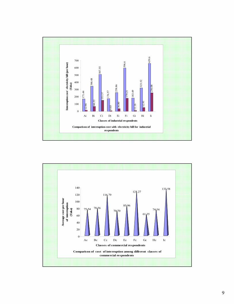
9

Comparison of interruption cost with electricity bill for industrial respondents

171.

44

346.

48

507.

55

176.

57 258.

86

596.

6

183.

49

323.

52

659.

6

12.9

4 66.3

3 153.

37

9.85 36

.80

179.

21

11.1

6 52.9

1

256.

08

0

100

200

300

400

500

600

700

Ai Bi Ci Di Ei Fi Gi Hi Ii

Classes of industrial respondents

Iinte

rrup

tion

cost

/ el

ectr

icity

bill

(per

hou

r)

(Tak

a)

75.54 78.56

116.79

70.70

85.96

125.27

61.3574.34

133.58

0

20

40

60

80

100

120

140

Ave

rage

cos

t per

hou

r of

int

erru

ptio

n

(Tak

a)

Ac Bc Cc Dc Ec Fc Gc Hc Ic

Classes of commercial respondents

Comparison of cost of interruption among different classes of commercial respondents

10

Comparison of interruption cost with electricity bill among different classes of commercial respondents

75.5

4

78.5

6

116.

79

70.7

85.9

6

125.

27

61.3

5 74.3

4

133.

58

2.49 3.74 12

.35

2.11

13.8

3

1.18 2.79 12

.75

5.01

0

20

40

60

80

100

120

140

160

Ac Bc Cc Dc Ec Fc Gc Hc Ic

Classes of commercial respondents

Inte

rrup

tion

cost

per

hou

r

and

hour

ly a

vera

ge e

lect

ricity

bill

(Tak

a)

Correlation between interruption costs and system reliability

0

50

100

150

200

250

300

350

400

60 65 70 75 80 85 90 95 100

System reliability (%)

cos

t per

hou

r of i

nter

rupt

ion

(Tak

a)

Industrial

Commercial

Residential

11

Comparison of interruption cost with the electricity bill for Residential Consumers

0.94.668.3810.3944.1857.08

Tk/hour of interruption

Tk/interruptionTk/hour of interruption

Tk/interruptionTk/hour of interruption

Average electricity

bill (Tk/hour of energy consumpti

on)

Without inconvenien

ce and damage of appliance

costs

Without inconvenience cost

Incorporating all Cost components

Average cost of interruption

Comparison of the Evaluated Interruption Cost with that of North American Utilities

Utility

Sector of consumer

Residential Industrial Commercial

Averageoutage

cost($/kwh)

Average outage

cost (taka/kwh)

Average outage

cost($/kwh)

Averageoutage

cost(taka/kwh

)

Averageoutage

cost($/kwh)

Average outage

cost (taka/kwh)

American 1 0.60 34.80 7.20 417.60 8.40 487.20

Canadian 1 0.46 26.68 15.24 883.92 15.78 915.24

DESA, Bangladesh

0.25 14.50 0.08 4.65 0.36 20.70

12

GENERATION EXPANSION PLANNING PROCESS

Forecasted demand

•construction time

• availability of sites

•availability of fuel

Planning analysis

A number of alternative plans

Comparison with desired level of

reliability

Final plan

Analysis of financial and environmental impacts

Economic analysis

Plans with desired level of reliability

Reliability analysis

Comparison with desired level of

reliability

Plans those do not satisfy desired level of

reliability

Rejected plans

Plans for modificationTechnical viability

CONCLUSIONS

BY PROPERLY EVALUATING THE LOSS DUE TO POWER INTERRUPTION THE OPTIMAL LEVEL OF SYSTEM RELIABILITY MAY BE EVALUATED.

PRESENT ELECTRICITY TARIFF IS MUCH LOWER THAN THE LOSS DUE TO POWER INTERRUPTION.

1

DECISION VARIABLES FOR THE OPTIMAL RELIABILITY LEVEL OF AN

UTILITY




TH

ASI

A R

EG

ION

AL

INIT

IAT

IVE

/EN

ER

GY


CONTENTS

FACTORS AFFECTING SYSTEM RELIABILITY .

IMPACTS OF FOR, UNIT SIZE AND RELIABILITY LEVEL ON SYSEM RESERVE AND ALLOWABLE PEAK DEMAND.

IMPACTS OF LOAD MANAGEMENT SCHEMES ON SYSTEM RELIABILITY.

RELIABILITY BENEFITS OF INTERCONNECTION WITH NEIGHBORING UTILITIES.

CONCLUSIONS.

2

FACTORS IMPROVING SYSTEM RELIABILITY

Forced outage rate (FOR) of generating unit

Selection of unit size

Interconnection with neighboring utilities

Application of load management schemes

UP TIMEm1

FailureRepair

m2 m3

r1 r2

DOWN TIME

TIME

DOWN

States of generatingunit

UP

EFFECT OF FOR

FIG. RUN-FAIL-REPAIR-RUN CYCLE OF A GENERATING UNIT

3

m = Mean up time =

r = Mean down time =

λ = Unit failure rate =

µ= Unit repair rate =

Forced outage rate = FOR = q =

FOR can be reduced byReducing DOWN time with improved repair facilities

Increasing UP time with proper maintenance and using quality devices

∑i

imN1

∑i

irN1

m1

r1

µλλ+

EFFECT OF FOR

Unit Size (MW) FOR LOLP Reserve (MW)

100 0.01 629

100 0.05 1408

100 0.10 2182

100 0.20 3484

[FOR A SYSTEM OF IC=10,000 MW]

⎪⎪

⎭

⎪⎪

⎬

⎫

×

×

×

×

−

−

−

−

4

4

4

4

104104104104

4

6000

7000

8000

9000

0.01 0.05 0.1 0.2

FOR

EFFECT OF FOR (CON’D)

EFFECT OF UNIT SIZE


50 0.05 1114

100 0.05 1408

200 0.05 1919

500 0.05 2984


⎪⎪

⎭

⎪⎪

⎬

⎫

×

×

×

×

−

−

−

−

4

4

4

4

104104104104

= 0.96 daysin 10 years

5

6800

7300

7800

8300

8800

50 100 200 500

Unit size (MW)

Max

imu

m a

llow

able

pea

k (M

W)

EFFECT OF UNIT SIZE (CON’D)

EFFECT OF LOLP


100 0.05 1 x 10-4 (0.96 days/10 years) 1536

100 0.05 2 x 10-4 (1.92 days/10 years) 1480

100 0.05 4 X 10-4 (3.84 days/10 years) 1408

100 0.05 8 x 10-4 (7.68 days/10 years) 1338


6

8500

8700

8900

0.0001 0.0002 0.0004 0.0008

LOLP

EFFECT OF LOLP (CON’D)

LOAD MANAGEMENT

Load management is the deliberate control or influencing of customer load in order to alter the pattern of electricity use by time-shifting some of the deferrable loads

BASIC APPROACHES OF LOAD MANAGEMENT

DIRECT CONTROL

INDIRECT CONTROL OR CUSTOMER INCENTIVES

ENERGY STORAGE

7

0

20

40

60

80

100

0 3 5 8 12 11 15 20 25

Percent reduction in Peak load

Per

cent

red

uctio

n in

LO

LP o

ver

base

cas

e

Direct LM 17to 23 hrs

Direct LM 18to 22 hours

EFFECT OF DIRECT LOAD CONTROL (LOAD REDUCED)

0

20

40

60

80

100

100 90 85 80 75 70

Prefixed value (in percent of peak load)Per

cent

red

uctio

n in

LO

LP o

ver

base

cas

e

EFFECT OF DIRECT LOAD CONTROL (CONSTANT PEAK)

8

0

10

20

30

40

50

60

70

80

90

100

0 5 8 10 15 20 25 30

Percent reduction in peak load

perc

ent r

educ

tion

in L

OLP

ove

r ba

se

case

EFFECT OF INDIRECT LOAD CONTROL

0

20

40

60

80

100

Pump ef f iciency75%



10 3020

-200

-400

-600

∼∼ Percent reduction in peak loads

Fig. Impacts of Energy Storage Scheme on Reliability

9

RELIABILITY BENEFITS OF INTERCONNECTION: BASIC CONCEPT

Utility X

Utility Z

Utility Y

CONFIGURATION 1: ALL UTILITIES ARE ISOLATED

TIE LINE ZY

TIE LINEX Z

CONFIGURATION 2: BILATERAL INTERCONNECTION

TIE LINEX Y

BASIC CONCEPT (cont’d)

10

TIE LINE TIE LINE

TIE LINEX

Z

Y

CONFIGURATION 3: ALL UTILITIES ARE INTERCONNECTED

BASIC CONCEPT (cont’d)

CONFIGURATION 1: ALL UTILITIES ARE ISOLATED

X Y Z

TABLE: GENERATION AND LOAD DATA

FOR

Z

80.1018

X

Capacity (MW)

Description of generation

Y

0.2 1020

Utility LOAD

(MW)

21 0.15 12

11

= Loss of load

= Demand met

= Available generation

510

15

20MW

58

18

90

MW

512

15

21

20 40 60 85 100Time in percent

MW

FIG: SCHEMATIC OF AVAILABLE GENERATION AND DEMAND MET

Utility X

Utility Y

Utility Z

80

Fig: Duration of loss of load when utilities

are isolated

Dur

atio

n of

loss

of

load

(L

OLP

)

(tim

e in

%)

20

10

15

02468

101214161820

X Y Z

Utilities

12

CONFIGARATION 2: BILATERAL INTERCONNETION

TABLE: CAPACITY STATE TABLE

ON 72ON8

UTILITY X UTILITY Y

OFFON

STATE OF GENERATION DURATION (PROBABILITY)

(TIME IN PERCENT)

ON 18OFFOFF 2OFF

FIG: UTILITYES X AND Y ARE INTERCONNECTED

GEN: 20 MW,

FOR=0.2

LOAD= 10MW

TIE LINEGEN: 18 MW,

FOR=0.1

LOAD= 8MWY

X

= Export

= Import

= Loss of load

LOLPX = 2%

LOLPY = 2%

510

15

20

20 40 60 72 100Duration (%)

MW

58

1518

20 40 60 100Duration (%)

MW

80 98

FIG: SCHEMATIC OF AVAILABLE GENERATION AND DEMAND MET

WHEN UTILITIES X AND Y ARE INTERCONNECTED

Utility X

Utility Y

72

18

= demand met by its own generation

= Available generation

13

20

10

15

2 2

15

20

10

15

20

1.5

15

0

5

10

15

20

ISOLATED X&Y X&Z Y&Z

XYZ

Fig: Comparison of loss of load: isolated utilities and bilateral

interconnection

Bilateral interconnection

Dur

atio

n of

loss

of l

oad

(LO

LP)

(tim

e in

%)

CONFIGARATION 3: MULTILATERAL INTERCONNECTION

Table: capacity state table

UTILITY X UTILITY Y

STATE OF GENERATION DURATION (PROBABILITY)

(TIME IN PERCENT)UTILITY Z

ONON ON

ON

61.2

OFF

OFF

OFF

ON

ON

OFF

OFF

OFF

ON

ON

ON

OFF

OFF

ON

OFF

ON

OFF

ON

OFF

OFF 1.2

6.8

10.8

15.3

2.7

1.7

0.3

GEN: 20 MW,

FOR=0.2

LOAD= 10MW

GEN: 21 MW,

FOR=0.15

LOAD= 12MW

GEN: 18 MW,

FOR=0.1

LOAD= 8 MW

Fig: All three utilities are interconnected

TIE LINE

(Infinite capacity)

14

CONFIGARATION 3: MULTILATERAL INTERCONNECTION


1.2

10010 40 50 60 8020 30 69.2 95.3

51015

20MW

6.810.8

61.2

0..3

2.7

10010 40 50 60 8020 30 69.2 95.3

58

1520MW

Y

1.7

10010 40 50 8020 30 69.2 95.3

5

1215

20MW

Fig: schematic of available generation and demand met when all utilities are interconnected

Time (%)

= generator available

61.2

61.2 62.4

X

= Export

= Import

= Loss of load

98

Configuration 3: Multilateral interconnection (cont’d)

20

10

15

38.8

2 2

1516.720

10

15

38.8

20

1.5

15

32

20.03

4.2 5.9

0

5

10

15

20

25

30

35

40

ALL AREISOLATED

X AND YCONNECTED

X AND ZCONNECTED

Y AND ZCONNECTED

ALL AREINTERCONNECTE

X

Y

Z

G

Fig: Comparison of loss of load for different configurations

Dur

atio

n of

loss

of l

oad

(LO

LP) (

time

in %

)

15

NR

WR

SR

ERNER

Ennore

KudankulamKayamkulam

Partabpur

Talcher/Ib Valley

Vindhyachal

Korba

MAJOR ENERGY RESOURCES IN INDIA

LEGEND

Coal

Hydro

Lignite

Coastal

Nuclear

VizagSimhadri

Kaiga

Tarapur

Mangalore

Krishnapatnam

RAPP

53,000MW

23,000MW

1,700MWSIKKIM

MYA

NMM

AR

CHICKEN NECK

Cuddalore

SRI LANKACOLOMBO

NEPALBHUTAN

DESHBANGLA

South Madras

Pipavav

Generation Load-Centre

Kolkata

Bhubaneswar

PatnaLucknow

Delhi

Mumbai

Chennai

Bangalore

Bhopal

Guwahati

Jammu

Ludhiana

Jaipur

Gandhinagar

Indore

Raipur

Thiruvananthapuram

Kozhikode

Hyderabad

* Hydro Potential : 1,10,000> 25,000MW already installed

> 19,000MW under implementation

> 66,000MW still to be exploited

* 90% coal reserves in ER & WR

EXPECTED BENEFITS OF INTERCONNECTION IN SOUTH ASIA

% OF THE POTENTIAL

(MW)

56.4511292000Sri Lanka

13.06496338000Pakistan

0.4436883290Nepal

33.72540775400India

1.4844430000Bhutan

65.71230555Bangladesh

ALREADY HARNESSEDPOTENTIAL(MW)

COUNTRY

HYDRO ELECTRIC POTENTIAL IN SOUTH ASIA

16

Initial data

1.116002829Sri Lanka

1.11400019500Pakistan

1.085501126Nepal

1.0582000102800India

1.01004409Bhutan

1.132005230Bangladesh

Load growth (%)

Initial peak demand (MW)

Initial installed capacity (MW)

Country

Unserved energy cost

0.00E+00

5.00E+08

1.00E+09

1.50E+09

2.00E+09

2.50E+09

3.00E+09

3.50E+09

1 2 3 4 5

Period

Cos

t in

$

Full trade

No trade

17

Total cost comparison (2003 - 2013)

7.30E+10

7.40E+10

7.50E+10

7.60E+10

7.70E+10

7.80E+10

7.90E+10

8.00E+10

8.10E+10

8.20E+10

8.30E+10

Cos

t in

$

Full trade 7.63E+10 8.20E+10

1 2

CONCLUSIONS

In expansion planning, factors, like unit size, interconnection, and load management schemes should duly be considered to improve the system reliability or to maintain the standard level of reliabilityHigher unit size should be avoided, in generation expansion, if it does not affect the economy.Interconnection with the neighboring utilities improves the system reliability.Load management is an option deserves to be considered when other options have problems to be implemented or fail to achieve desired level of reliability.Quick repair of faulty devices improves system reliability.

1

LOAD CARRYING CAPABILITY OF NEWLY ADDED GENERATING

UNIT/UNITS: RELIABILITY ASPECTS




TH

ASI

A R

EG

ION

AL

INIT

IAT

IVE

/EN

ER

GY


CONTENTS

EVALUATION TECHNIQUE OF LOAD CARRYING CAPABILITY (LCC) OF A GENERATING UNIT

IMPACTS OF FOR ON LCC

CONCLUSIONS

2

GENERATION MODEL

Capacity FOR

20 0.1

30 0.2

LOAD (MW)

30

% of time

LOAD MODEL

100%

ILLUSTRATION OF EVALUATION PROCEDURE OF LOAD CARRYING CAPABILITY (LCC) OF A

GENERATING UNIT

CAPACITY OUTAGE TABLE

Capacity Available Exact Cumulative

Out (MW) Capacity Probability Prob.

0 50 0.72 1.0

20 30 0.08 0.28

30 20 0.18 0.20

50 0 0.02 0.02

LOLP = Pr. (AC < PK) = 0.2

3

CAPACITY OUTAGE TABLE ( WITH AN ADDITIONAL UNIT OF 40 MW AND FOR OF 0.1)

Capacity on Available Cumul. outage (MW) Capacity Probability Prob.

0 90 0.648 1.020 70 0.072 0.35230 60 0.162 0.2840 50 0.072 0.11850 40 0.018 0.046

60 30 0.008 0.02870 20 0.018 0.02

90 0.0 0.002 0.002

FOR A PEAK OF 30 MW, LOLP = 0.02FOR LOLP = 0.2 60 < PEAK < 50∴ 20 < LCC < 30

0

0.1

0.2

0.3

0.4

0.5

0.6

0.7

0.8

0.9

1

0 10 20 30 40 50 60 70 80 90

AC

Com

Pro

b.

q=0.1 q=0.2

q=0.3 q=0.4

q=.05

With initial units

With additional unit (Cap=40 MW, FOR= 0.1 TO 0.5 )

EFFECT OF FOR ON LCC

4

FOR LCC (MW)

0.5 11.5

0.4 12

0.3 14

0.2 19

0.1 25.5

IMPACTS OF FORS ON LCC

CHANGES IN LCC IN A REALISTIC SYSTEMIC = 10,100 MW

Highest unit capacities 300 MW and 500 MW

LOLP = 0.1 day/year

Changing FOR of 300 MW and 500 MW only

--111213313404493579661739815

9006889587938693860285138427834582678191

456789

10111213

Reduction in peak carrying capacity (MW)

Peak load carrying capacity (MW)

FOR (%)

5

The above table shows the change in LCC for FOR values from 4% to 13%.

The decrease in LCC is 815 MW.

If the forecasted peak is 9006 MW and the FORs of large units are 13% then the system would have to install approximately 815 MW additional capacity to maintain LOLP (a reliability level of ) 0.1 day/year

CONCLUSIONS

• LCC is an useful measure to system planners to see the relative impact of new units in satisfying system load growth

• System with units of higher FORs requires higher installed capacity to meet the system demand (peak).

1

EVALUATION TECHNIQUES OF RELIABILITY LEVEL OF A SINGLE AREA

UTILITY




TH

ASI

A R

EG

ION

AL

INIT

IAT

IVE

/EN

ER

GY


CONTENTS

DIFFERENT RELIABILITY INDICES

DESCRIPTION OF DIFFERENT STEPS OF RECURSIVE METHOD

DEFFERENT TECHNIQUES OF DEVELOPING CAPACITY OUTAGE TABLE

EVALUATION OF LOLP

SEGMENTATION METHOD AND ITS ILLUSTRATION

2

RELIABILITY INDICES

Loss of Load Probability (LOLP)

Loss of Energy Probability (LOEP)

Frequency and Duration (FAD)

Monte Carlo Simulation (MCS)

METHODOLOGIES

Recursive (Booth –Baleriaux Technique) Method

Cumulant Method

Segmentation Method

DIFFERENT STEPS OF RECURSIVE METHOD

DEVELOP A CAPACITY OUTAGE TABLE OF THE GENERATING SYSTEM USING EITHER THE OUTAGE CAPACITY BUILDING ALGORITHEM OR BY USING THE RECURSIVE FORMULA.

INSERT THE AVAILABLE CAPACITY COLUMN OBTAINED FROM CAPACITY OUTAGED STATE AND THE INSTALLED CAPACITY .

ALSO INSERT A CUMULATIVE PROBABILITY COLUMN USING THE EXACT PROBABILITY VALUES (IF RECURSIVE FORMULA IS NOT USED).

FOR EACH LOAD LEVEL FIND THE LOLP CONSIDERING THAT LOLP = PROBABILITY {AVAILABLE CAPACITY < LOAD} FROM THE CUMULATIVE PROBABILITY COLUMN

3

MULTIPLY EACH LOLP VALUE OBTAINED FOR A GIVEN LOAD LEVEL BY THE PROBABILITY OF THE OCCURRENCE OF THAT LOAD

SUM THE PRODUCT OF LOLP CORRESPONDING TO EACH LOAD LEVEL AND THE PROBABILITY OF OCCURRENCE OF THAT LOAD TO GET THE FINAL VALUE OF LOLP

GENERATION MODELCapacity (MW) FOR

200 0.02

300 0.03

400 0.04

LOAD MODELLoad level (MW) No. of occurrence (days)

650 5

550 5

450 5

350 5

EXAMPLE CLARIFYING METHODOLOGY

4

GRAPHICAL REPRESENTATION OF GENERATION MODEL

0 200 0 300

Capacity on outage (MW) Cap on outage (MW)

0 300

Capacity on outage (MW)

0.97

0.03FOR = q = 0.02

P =0.98

Probability

0.04

0.96

GRAPHICAL REPRESENTATION OF LOAD

0 5 10 15 20Time (Days)

650

550

450

350

LOAD

(MW)

350 450 550 650

Probability5/20 5/20 5/20 5/20

LOAD (MW)

Probability Density Function of Load

5

CAPACITY OUTAGE TABLE( State Enumeration Technique )

STATES OF UNITS

UNIT UNIT UNIT CAPACITY ON PROBABILITY OF OCCURRENCE

# 1 # 2 # 3 OUTAGE (MW)

ON ON ON 0 0.98 x .97 x .96 = 0.912576

DOWN ON ON 200 0.018624

ON DOWN ON 300 0.028224

ON ON DOWN 400 0.038024

DOWN DOWN ON 500 0.000576

DOWN ON DOWN 600 0.000776

ON DOWN DOWN 700 0.001176

DOWN DOWN DOWN 900 0.000024

CAPACITY OUTAGE TABLE BUILDING ALGORITHM

0.98

0.02

This density function can be expressed in the form of

0 200 a Capacity Outage Table

Capacity on outage (MW) Probability

0 0.98

200 0.02

Table 1MW

Prob.

6

To incorporate 2nd unit

First , Considering 2nd. Unit in Service

Table – 2Capacity on Outage (MW) Probability

0 + 0 = 0 0.98 x .97 = 0.9506

200 + 0 = 200 0.02 x .97 = 0.0194

Outage Cap.(MW)

Prob..97

0.03

Next, Considering 2nd Unit (300 MW) out of Service

Table - 3


0 + 300 = 300 0.98 x .03 = .0394

200 + 300 = 500 0.02 x .03 = .0006

Combining Tables 2 and 3, one gets

Table – 4Capacity on outage (MW) Probability

0 0.9506

200 0.0194

300 0.0294

500 0.0006

7

To in corporate the 3rd Unit (400 MW, FOR = 0.04)

Follow the above procedure

Table – 5 ( Considering 400 MW Unit in service)


0 + 0 = 0 0.9506 x .96 = 0.912576

200 + 0 = 200 0.0194 x .96 = 0.018624

300 + 0 = 300 0.0294 x .96 = 0.028224

500 + 0 = 500 0.0006 x .96 = 0.000576

Table – 6 (Considering 400 MW Unit out of service)

Capacity on outage (MW) Probability0 + 400 = 400 0.9506 x .04 = 0.038024

200 + 400 = 600 0.0194 x .04 = 0.000776

300 + 400 = 700 0.0294 x .04 = 0.001176

500 + 400 = 900 0.0006 x .04 = 0.000024

Combining Tables 5 and 6 and reordering capacity states

Table – 7Capacity on outage (MW) Probability

0 0.912576

200 0.018624

300 0.028224

400 0.038024

500 0.000576

600 0.000776

700 0.001176

900 0.000024

8

Introducing available capacity and cumulative probability columns Table – 7 becomes

Capacity on Available capacity Exact CommutativeOutage (MW) (MW) Probability Probability

0 900 0.912576 1.0200 700 0.018624 0.087424300 600 0.028224 0.068800400 500 0.038024 0.040576500 400 0.000576 0.002552600 300 0.000776 0.001976700 200 0.001176 0.001200900 00 0.000024 0.000024

TABLE 8

The above table can also be obtained using a recursive formula

P(X) = (1 – q) P′ (X) + q P′ (X′ – c)

Where,

P’(X) = Cumulative probability of X MW or greater before the unit of C MW is addedP(X) = Cumulative probability of X MW or greater after the unit of C MW is added

⎭⎬⎫

⎩⎨⎧ ≤×

=wiseother

ifXP

001

)('

9

Load Probability of Reserve available LOLP (For individual load) Level Occurrence Capacity (MW)

350 5/20 550 0.001976 x

450 5/20 450 0.002552 x

550 5/20 350 0.040576 x

650 5/20 250 0.057424 x

LOLP = 0.028476

205

205

205

205

EVALUATION OF LOLP

SEGMENT METHOD

Concept behind segmentation method

For binary state model of a generating unit the convolution of the PDF of the outage capacity of a generating unit with the PDFload can be expressed as

qCLefplflef LLLe )()()( −+=

10

l1 l2 l3 l1+c l2 +c l3 +c

l1 l2 l3

Le

fL(l)

PL1 PL2PL3

LOutage capacityo c

p q

Pl1P Pl2P Pl3PPl1q Pl2q

Pl3q

PDF AFTER CONVOLUTION

PDF OF LOADPDF OF CAPACITY ON OUTAGE

Probability

*

DIFFERENT STEPS OF SEGMENTATION METHOD

Obtain the PDF of load by sampling the chronological historical or forecasted load.

Construct segments by dividing demand axis. The segment size is equal to the highest common factor of the generating unit capacities.

Obtain the distribution of segment by translating the PDF of load into the PDF of segment. This is done by simply attaching a probability to a segment, which is equal to the sum of probabilities of the load impulses lying in the range of that segment.

Convolve the PDF of each generating unit one by one with the PDF of segments. The convolution procedure requires.

Multiplication of the distribution of segments by the availability of the unit.

Shifting the original distribution of segments towards right by an amount equal to the capacity of the unit being convolved.

Multiplication of the shifted distribution by the unavailability of the unit.

Addition of the above two products to get the final distribution after convolution.After convolving all the units in the system LOLP is evaluated. LOLP is equal to theprobability value of the last segment in the final distribution.

11

c = Segment Size = Highest common factor of ( 200, 300, 400) =100

N = Number of segments =200 300 400 1 10

100+ +

+ =

0.250.250.250.25Shift= 200

0.0050.0050.250.250.2450.245

.25+.005+.005.25.245.245300 x .03

x 0.97

x 0.02

x 0.980.250.250.250.25

MWInstalled Capacity

0 100 900300 600

ILLUSTRATION OF METHODOLOGY

.0078.01235.0122.24985.2425.23765.23765 x .96

0.5247.23765.23765

x .04

0.0284760.0213620.021218

0.239856

0.23280.228144

LOLP = 0.028476

400 MW

0 100 300 600 900

MW

12

CONCLUSIONS

RECURSIVE AND SEGMENTATION METHODS FOR THE EVALUATION OF RELIABILITY INDEX, LOLP, FOR A SINGLE AREA SYSTEM ARE ILLUSTRATED THROUGH EXAMPLE

SEGMENTATION METHOD IS CONCEPTUALY STRAIGHT FORWARD

SEGMENTATION METHOD IS ALSO COMPUTATIONALY SIMPLE

1

EVALUATION TECHNIQUES OF RELIABILITY LEVEL OF

INTERCONNECTED UTILITIES




TH

ASI

A R

EG

ION

AL

INIT

IAT

IVE

/EN

ER

GY


CONTENTS

CAPACITY TRANSACTION DEPENDING FACTORS

DESCRIPTION OF SEGMENTATION METHOD FOR INDEPENDENT LOAD

EXAMPLE CLARIFYING METHODOLOGY FOR INDEPENDENT LOAD

DESCRIPTION OF SEGMENTATION METHOD FOR CORRELATED LOAD

EXAMPLE CLARIFYING METHDOLOGY FOR CORRELATED LOAD

2

Utility X Utility Y

TIE LINE

CAPACITY TRANSCTION BETWEEN THE INTERCONNECTED SYSTEMS DEPENDS ON

TIE LINE CAPACITY

DEMAND OF THE EXPORTING SYSTEMDEMAND OF THE IMPORTING SYSTEMAVAILABLE GENERATING CAPACITY OF THE EXPORTING SYSTEM

THE INCORPORATION OF THE ABOVE CONSTRANTS AND KEEPING THE INDENTITY OF EACH INDIVIDUAL UTILITY MAKE THE EVALUATION PROCEDURE OF INTERCONNECTED SYSTEM DIFFERENT FROM THAT OF THE SINGLE AREA SYSTEM

DIFFERENT STEPS OF SEGMENTATION METHOD FOR THE EVALUATION OF RELIABILITY INDICES OF TWO

NTERCONNECTED SYSTEM IN CASE OF UNCORRELATED (INDEPENDENT) LOAD

Develop the probability density function (PDF) of load .

Construct segments of equal size by dividing the demand axis. The segment size is the highest common factor of the generating units and tie line capacities. The total number of segments is equal to the installed generating unit capacity divided by the segment size plus one.

Obtain the distribution of segments by translating the PDF of load into that of segment . The probability of a segment is equal to the sum of the probabilities of the load impulses lying in the range of the segment.

Convolve the PDFs of all generating units of a system with that of the segment one by one. To do so,

Multiply the distribution of segments by the availability ofthe unit, i.e. (1 –FOR), being convolved.

3

Shift the original distribution of segments towards right by an amount equal to the capacity of the unit being convolved.

Multiply the shifted distribution by the FOR of the unit.

Obtain the distribution of segments after convolution by adding the above two product.

Form the joint PDF of segments (Venn diagram) by using the PDF of segments of each system obtained after convolving all the units in that system.

Integrate the different zones of Venn diagram to obtain the different reliability indices.

0

40

30

20

10

1 2 3 4

Utility 1

Utility 2

LOAD

(MW

)

TIME (HOURS)

FIG: HOURLY LOAD PROFILE

Table: Generating system description

Utility 1No of units Capacity (MW) FOR

2

30 0.1

0.2

1

10

Utility 2No of units Capacity (MW) FOR

2

25 0.3

0.1

1

15

EXAMPLE FOR CLARIFICATION (INDEPENDENT LOAD)

4

SEEGMENTATION METHOD (CON’D)(FOR INDEPENDENT LOAD)

FIG: PDF of load for utility 1

10 20 30 40

1/4 1/41/4 1/4

Pro

babi

lity

Load (MW)

.08.096.096.1.1.324.324.864.864.576.576

.8.96.96.64.6430 MW X.1

.04.04.36.36.96.96.64.64 X.9

.2.211.8.810 MW X.2

.2.211.8.8 X.8

111110 MWSHIFT X.2=FOR

111110 20 30 40 50 60

TCIC1

X.8 =(1-FOR)

Fig: schematic of convolution procedure of system 1 (all numbers in the boxes to be divided by 4)

0

40

30

20

10

1 2 3 4

Utility 1LOA

D (M

W)

TIME (HOURS)FIG: HOURLY LOAD PROFILE

SEGMENTATION METHOD (FOR INDEPENDENT LOAD) (CON’D)

0.0006350.0014850.0003050.001880.001250.0018450.0034650.000630.0028350.002840.00284

0.0007620.0017820.0003660.002260.00150.0022140.0041580.0007560.0034020.00340.0034

0.0007620.0017820.0003660.002260.00150.0022140.0041580.0007560.0034020.00340.0034

0.0007940.0018560.0003810.002350.0015630.0023060.0043310.0007880.0035440.003540.00354

0.0007940.0018560.0003810.002350.0015630.0023060.0043310.0007880.0035440.003540.00354

0.0025720.0060140.0012350.007610.0050630.0074720.0140330.0025520.0114820.011480.01148

0.0025720.0060140.0012350.007610.0050630.0074720.0140330.0025520.0114820.011480.01148

0.0068580.0160380.0032940.02030.01350.0199260.0374220.0068040.0306180.030620.03062

0.0068580.0160380.0032940.02030.01350.0199260.0374220.0068040.0306180.030620.03062

0.0045720.0106920.0021960.013540.0090.0132840.0249480.0045360.0204120.020410.02041

0.0045720.0106920.0021960.013540.0090.0132840.0249480.0045360.0204120.020410.02041

FIG: SCHEMATIC REPRESENTATION OF JOINT PROBABILITIES (VENN DIAGRAM) (ALL NUMBERS INSIDE THE BOX BE DIVIDED BY 4X4 AND ALL PROBABILITY VALUES OF THE VECTORS BE DIVIDED BY 4)

TCIC1

10 3020 604015 50

0.020.0240.0240.0250.0250.810.0810.2160.2160.1440.144

25

35

45

55

650.03175

0.07424

0.01525

0.094

0.0625

0.09225

0.17325

0.00315

0.14175

0.14175

0.14175

5

LOLP1 = 0.272/4= 0.068

LOLP2 = 0.485/4= 0.12125

LOLP1/2 =

LOLP1/2 =

031832.044

0.28120.0240.0360.0360.13192 =++++

X

0419297.044

0.4734560.02970.02970.00610.13192 =++++

X

LOLPG = (.031832+.0419297)-0.13192=0.065516

.4853.515

.2723.728

.473456

.0297.0297

.13192.0061

.036.036

.024

.2812

.08.096.096.1.1.324.324.864.864.576.576

10 20 30 40 50 60

.127

.297

.061

.376

.25

.369

.693

.126

.567

.567

.567 15

25

35

45

55

65

IC1 TC

Fig: schematic representation of joint probabilities (all numbers inside the joint probability matrix to be divided by 4x4 and all the probability values of the vectors outside the matrix to be divided by four)

IC2

TC

Some of the probabilities

DIFFERENT STEPS OF SEGMENTATION METHOD FOR THE EVALUATION OF RELIABILITY INDICES OF

TWO INTERCONNECTED SYSTEM IN CASE OF CORRELATED DEMAND.

Develop the joint PDF of load

Construct two dimensional segments by dividing X and Y axes forming segments of square size. That is all four sides of a segment are equal in size and each side is equal to the highest common factor of generating unit capacities of both systems and the tie line capacity. The total number of divisions of an axis is equal to the installed capacity of a system to which the axis is assigned plus tie line capacity divided by the segment size plus one.

Obtain the PDF of segment by translating the joint PDF of load. The probability of a segment is equal to the sum of the probabilities of the load impulses lying in the range of that segment.

6

Shift the original PDF, i.e, before multiplying by (1-q) in the above step.The amount of shift is equal to the capacity of the unit being convolved. The direction of shift depends on the system to which the convolving unit belongs to.If the unit belongs to a system which is assigned to x-axis, the direction of shift will be towards x-axis, otherwise the shift will be towards Y- axis.

Multiply the shifted distribution by the unavailability of the unit, q

Obtain the distribution of segments after convolution by adding the above two products.

Integrate the different zones of the probability mass, evolved after convolving all the units of both systems, to obtain the different probability indices.

SEGMENTATION METHOD FOR CORRELATED LOAD

0

40

30

20

10

1 2 3 4

Utility 1

Utility 2

LOAD

(MW

)

TIME (HOURS)FIG: HOURLY LOAD PROFILE OF TWO UTILITIES

Fig: joint PDF OF loads of two utilities

LOAD OF UTILITY 1

Probability

Load

of ut

ility 2

55

10 2015 25 30 35 40

40

1015

2025

3035

1/4

1/4

1/4

1/4

EXAMPLE FOR ILLUSTRATION

7

SEGMENTATION METHOD FOR CORRELATED LOAD (CONT’D)

1

1

1

1

10

65

55

45

35

25

20 30 40 50 6015

TCIC1

IC2

TC

System 1 (MW)S

yste

m 2

(M

W)

Fig: joint probability matrix for systems with correlated load (all numbers in the boxes to be divided by 4).

PROCESS OF CONVOLUTION

10

65

55

45

35

25

20 30 40 50 6015

TCIC1

IC2

TC

System 1 (MW)

Sys

tem

2 (

MW

)

Fig: Unshifted distribution of segment multiplied by the availability of the unit (All numbers in the boxes to be divided by 4)

1

1

1

1

X (1-0.2)

8

10

65

55

45

35

25

20 30 40 50 6015

TCIC1

IC2

TC

System 1 (MW)S

yste

m 2

(M

W)

Fig: Shifted distribution of segments (Multiplied by FOR) (all numbers in the boxes to be divided by 4)

1

1

1

1

Shift

(10 MW= 2 segments)

X 0.2

0.8 0.2

0.20.8

0.8 0.2

0.20.8

10

65

55

45

35

25

20 30 40 50 6015

TCIC1

IC2

TC

System 1 (MW)

Sys

tem

2 (

MW

)

Fig: Joint probability Matrix after convolving one 10 MW unit of system 1 (all numbers in the boxes to be divided by 4).


9


LOLP1 = (0.03628+0.018144+----------+0.025204+0.074188)/ 4 = 0.068

LOLP2 = (0.031104+---------------+0.000252+0.118588+0.025204) / 4 = 0.12125

LOLP1/2 = (0.025204+0.074188+0.000224+0.019584) /4 =0.0298

LOLP2/1 = (0.025024+0.118588+0.003456+0.015552+0.000252) /4 = 0.040763

LOLPG = (0.0298+.040763)-.0252044 =0.064262

.003456

.001944

.036288

.018144

.008064

.018144.004032

.008064.015552

.008224

.139968 .015552

.031104

.069984

.004032

.001944

.015552

.031004

0.118588

.015552.008748

.025204.000252.002016

.019584.000224

.074188.03628

10 20 30 40 50 6015

25

35

45

55

65

IC2

TC

IC1 TC

Fig: Joint probability matrix after convolving all the units of two utilities (all numbers in the boxes to be divided by 4)

CONCLUSIONS

CONSTRAINTS OF CAPACITY TRANSACTION MAKE THE EVALUATION OF INTERCONNECTED SYSTEM DIFFERENT FROM THAT OF A SINGLE AREA SYSTEM

AMONG DIFFERENT TECHNIQUES OF EVALUATION SEGMENTATION METHOD IS EASY TO IMPLEMENT

1

CAPACITY SAVINGS THROUGH INTERCONNECTION AND OPTIMAL TIE

LINE CAPACITIES




TH

ASI

A R

EG

ION

AL

INIT

IAT

IVE

/EN

ER

GY


CONTENTS

EVALUATION OF THE EQUIVALENT GENERATING UNIT CAPACITY

OPTIMAL TIE LINE CAPACITY EVALUATION THROUGH CASE STUDIES

IEEE RELIABILITY TEST SYSTEM

SMALL SYSTEM

2

ILLUSTRATION OF THE EVALUATION PROCEDURE OF A GENERATING UNIT CAPACITY EQUUIVALENT TO THE TIE LINE CAPACITY

SYSTEMA

SYSTEMB

TIE LINE

SYSTEM DATA

0101TIE LINE

CAPACITY

40600.020.02

1020

41B

50750.020.02

1025

51

A

PEAK LOAD(MW)

INSTALLED CAPACITY

(MW)

FORCAPACITY (MW)

NUMBEROF UNITS

SYSTEM

CAPACITY OUTAGE TABLE OF SYSTEM A

1.000000000.114157620.023765550.020076080.001997670.001922370.000077630.000076860.000001560.000001560.000000020.00000000

0.885842380.090392070.003689470.018078410.000075300.001844740.000000770.000075300.000000000.000001540.000000020.00000000

01020253035404550556575

Cum.probabilityIndividual probabilityCap.out (MW)

3

CAPACITY OUTAGE TABLE OF SYSTEM B

1.000000000.096079200.022289750.001583530.000046890.000000630.00000000

0.903920800.073789450.020706220.001536640.000046260.000000630.00000000

0102030405060

Cum. prob.Individual Prob.Cap.out (MW)

JOINT PROBABILITY DENSITY FUNCTION OF TWO INT. SYSTEMS

0.00000.00000.00000.00150.02070.07370.9039

6050403020100

0.000075

0.000065

0.000055

0.000050

0.000045

0.000040

0.001835

0.000030

0.018025

0.003620

0.090310

0.88580

0.00000.00000.00000.00000.00000.00000.0000

0.00000.00000.00000.00000.00000.00000.0000

0.00000.00000.00000.00000.00000.00000.0000

0.00000.00000.00000.00000.00000.00000.0000

0.00000.00000.00000.00000.00000.00000.0000

0.00000.00000.00000.00000.00000.00000.0000

0.00000.00000.00000.00000.00000.00010.0016

0.00000.00000.00000.00000.00000.00000.0000

0.00000.00000.00000.00000.00040.00000.0146

0.00000.00000.00000.00000.00400.00000.0099

0.00000.00000.00000.00010.01680.00980.0000

0.0000.00000.00000.00130.00450.05820.0000

RA = 25

(VENN DIAGRAM ) LOLPA/B = 0.00012042

RB = 20

4

PROBABILITY TABLE OF ASSISTANCE FROM SYSTEM B

0.022289750020

0.07378945101010

0.9039208020200

ProbabilityExpected Assistance from System B to System A (MW)

Reserve of System B

(MW)

Capacity outage of system B

(MW)

0.02228975

0.07378945

0.90392080

Probability

Capacity on outage (MW)

Probabilistic model of an equivalent assistance unit (From system B to System A)

0.02228975

0.97771025

Probability

Capacity on outage0 10

Probabilistic model of equivalent assistance unit incorporating tie line constraint

0 10 20

5

MODIFIED CAPACITY OUTAGE TABLE OF SYSTEM A INCLUDING EQUIVALENT ASSISTANCE UNIT

1.000000000.133902830.025780350.020158300.002482850.002327000.000120420.000117990.000003250.000003230.000000050.000000050.00000000

0.866097170.108122480.005622050.017675450.000155850.002206580.000002430.000114740.000000020.000003180.000000000.000000050.00000000

0102025303540455055606575

Cum. prob.Individual prob.Cap. out (MW)

LOLPA|B = Pr. {Cap out > Reserve} = 0.00012042

[Reserve = (75 + 10) – 50 = 35 MW]

The LOLPA|B obtained from the Venn diagram is same as obtained from the modified capacity outage table

IN THIS CASE A TIE LINE OF 10 MW CAPACITY WITH FOR = 0.0 IS EQUIVALENT TO A 10 MW UNIT OF FOR = 0.02228975

6

DEMAND DATA: 48-52 AND 1-8 WEEKS HOURLY LOADS OF IEEE-RTS

PEAK LOAD: 2850 MW, ENERGY : 4163.48 GWh

Type ofUnit

UnitSize

(MW)

No. ofUnits

FOR IncrementalCost

($/MWh)NuclearCoalCoalCoalOilOilOilOilHydro

40015035080

200100102050

241433546

0.120.040.080.020.050.040.020.100.01

5.59211.16011.40014.88219.87020.08028.55837.500

0.0

CASE STUDY


Utility 1Tie line

Utility 2

Type ofUnit

UnitSize

(MW)

No. ofUnits

FOR IncrementalCost

($/MWh)NuclearCoalCoalCoalOilOilOilHydro

50040035025035020050

100

12111243

0.130.130.130.080.140.100.110.01

4.50014.30015.10018.60030.40035.00043.200

0.0

HYPOTHETICAL SYSTEM

DEMAND DATA: 18-30 WEEKS HOURLY LOADS OF IEEE-RTS


CASE STYDY (CONT’D)

Utility 1Tie line

Utility 2

7

VARIAT ION OF LOLP G WIT H T IE LINE CAPACIT IES

-101234567

0 200 400 600 800

TIE LIN E C APAC ITIES (MW)

LO

LP

G (%

)



TABLE: RELIABILITY INDICES AT DIFFERENT TIE LINE CAPACITIES OF THE INTERCONNECTED UTILITIES

TIE LINE CAPACITY

(MW)

INDEPENDENT LOAD

LOLP1/2 LOLP2/1

0.0

100

200

300

400

500

600

700

.00274

.00143

.00079

.00050

.00037

.00032

.00031

.00030

.06543

.04533

.03026

.01942

.01219

.00775

.00505

.00337

CORRELATED LOAD

LOLP1/2 LOLP2/1

.00280

.00156

.00097

.00072

.00062

.00058

.00057

.00057

.06610

.04585

.03077

.02000

.01284

.00850

.00594

.00442

8

ENERGY GENERATION AND PRODUCTION COST OF INDIVIDUAL UTILITY AND OF GLOBAL SYSTEM

Table: Expected energy generation and production cost of two interconnected utilities (*pooling operation)

3949.52233785.30033634.04743507.39353409.96063348.72083311.49503296.8930

-------

4162.65054332.96534487.96334616.87584715.63514780.61784815.23364830.0331

--------

0.0100200300400500600700------------∝*

System 2System 1

Exp. Energy generation (GWh)

Tie Line Capacity

(MW)

44.59340.81937.52634.86432.84331.47830.70130.324

------

33.23435.55837.74439.59741.04442.03542.59842.867

------

System 2

System 1

Production cost (M$)

77.82876.37775.27074.46173.88873.51373.29973.192

73.093

15.45039.35695.61233.35372.02731.28440.89400.6991

0.5376

8112.17278118.26578122.01078124.26938125.59578126.33868126.72868126.9235

8127.0849

Production cost (M$)

Exp. Unservedenergy (GWh)

Exp. Energy generation

(GWh)

Global

Global production cost saving from interconnection

Fig: Global Expected saving and Expected unserved energy Vs. tie line capacity

0 200 400 600

73

74

75

76

77

78

Pro

duct

ion

Cos

t (M

$)

Tie Line Capacity (MW)

0

2

4

6

Exp

ecte

d S

avin

gs (M

$)

Saving

USE

9

11

Transmission Line Scenario

-----

_______

------

_______ 132 kV (existing)

132 kV (planned/ under construction

230 kV (existing)

230 kV (planned/under construction

LOLP for different tie line capacities

1.6402651.1614300.8271020.5777660.2970400.1633160.1268340.1203070.1197510.119732---------0.119732

1.1758050.8175270.5721980.3898230.1938880.1049230.0827290.0790140.0786880.078678------0.078678

0.4938900.3733320.2843330.2173720.1325820.0878220.0735350.0707220.0704930.070483------0.070483

1.1758051.1758051.1758051.1758051.1758051.1758051.1758051.1758051.1758051.175805----1.175805

0.4938900.4938900.493890 0.493890 0.4938900.4938900.4938900.4938900.4938900.493890- - --0.493890

0.010.020.030.050.075.0100.0125.0150.0175.0- - --∝

LOLPG (%)LOLP W|E(%)

LOLPE|W(%)

LOLPW(%)

LOLPE (%)Tie line capacity (MW)

10

0

200

400

600

800

1000

1200

1400

0 25 50 75 100 12 5 150 17 5 200

T ie line ca pacity (M W)

Perc

enta

ge d

iffe

ren

ce (

PD)

Percentage Difference in Global LOLP vs. Tie Line Capacity

Expected global savings (106 S)

Tie line capacity (MW)

Expected global unserved energy (MWh)

0 20010050 150

360

180

60

120

240

300

5

1

2

3

4Global savings

Global unserved energy

Expected global unserved energy and expected global savings vs. tie line capacity

11

CONCLUSIONS

INTERCONNECTION OPTION SHOULD BE EXPLORED IN GENERATION EXPANSION ANALYSIS IN PARALLEL WITH THE OPTION OF NEW CAPACITY ADDITION IN THE SYSTEM

EQUIVALENT GENERATING UNIT CAPACITY TO A TIE LINE CAPACITY MAY BE EASILY EVALUATED. THEN TWO OPTIONS, INTERCONNECTION AND INSTRALLATION OF NEW GEN. UNIT, SHOULD BE COMPARED

INCREASE OF TIE LINE CAPACITY BEYOND CERTAIN LIMIT DOES NOT IMPROVE SYSTEM RELIABILITY OR COST

1

MULTI AREA EVALUATION APPROACH IN A SINGLE AREA SYSTEM WITH LIMITED TRANSMISSION

CAPABILITIES




TH

ASI

A R

EG

ION

AL

INIT

IAT

IVE

/EN

ER

GY


CONTENTS

COMPARISON OF RELIABILITY INDICES OF A SYSTEM WITH LIMITED TRANSMISSION CAPACITY OBTAINED THROUGH SINGLE AREA APPROACH AND TWO AREA INTERCONNECTED APPROACH - AN ILLUSTRATIVE EXAMPLE

BANGLADESH POWER SYSTEM TREATED AS TWO AREA INTERCONNECTED SYSTEM TO EVALUATE ITS RELIABILITY INDICES

POWER SYSTEM OF INDIA: SHOULD IT BE TREATED AS A SINGLE AREA SYSTEM

CONCLUSION

2

L2L1

G2

G1 G3

LIMITED TRANSMISSION FACILITIES

A POWER SYSTEM WITH LIMITED TRANSMISSION FACILITY

Fig. 1: A Power System with limited Transmission Facility

L1 + L2

Fig.2: A Power System with no Transmission Constraint

System in Fig. 1 is not same as the system in Fig. 2 from reliability evaluation point of

view.

System in Fig. 1 resembles a two-area interconnected system

System in Fig. 2 resembles a single area system

Reliability evaluation techniques for the above two systems are different.

OBSERVATIONS

3

TIE

L1 L2System 1System 2

System Data of two interconnected system

55300.10.3

1525

212

50300.20.1

1030

211

Installed capacity (MW)

Peak Load(MW)

FORUnit capacity (MW)

No. of unitsSystem

CONSIDERING TWO INTERCONNECTED SYSTEM

Capacity Outage Table

0.567------

0.126---

0.2430.007

---0.054

------

0.003

0.576---

0.288---

0.036---

0.064---

0.032---

0.004---

05

10152025303540455055

System 2System 1ProbabilitiesCapacity on outage

(MW)

4

0.004--0.032--0.064--0.036--0.288

--0.576

50403020100

0.00855----------

0.0540----

0.00730

0.24325----

0.12615----------

0.5670

R=25 MW

TC=10 MW

0.000020.0000960.000190.000100.00030.00172

0.0002160.0012280.003450.001940.01550.03404

0.0000280.0002240.000480.000250.00200.00403

0.0009770.0077760.015550.008740.06990.13986

0.0005040.0040320.008040.004540.03620.07258

0.00280.018140.036280.020410.16330.32659

Joint Probability matrix (Venn diagram)

RELIABILITY INDICES

Loss of load probability(LOLP) of system 1 = LOLP1 = 0.1

LOLP of system 2 = LOLP2 = 0.064

LOLP of system 1 assisted by system 2 = LOLP1/2 = 0.0556

LOLP of system 2 assisted by system 1 = LOLP2/1 = 0.0580

LOLP of global system = LOLPG = 0.1072

5

CAPACITY OUTAGE TABLECONSIDERING SINGLE AREA SYSTEM

1.00.67340.51010.43750.41710.24090.20050.42600.07480.05800.03990.01860.01620.00700.00340.00230.00050.00030.00010.0000

0.32660.16330.07260.02040.17630.04030.07450.05130.01680.01810.02130.00240.00910.00370.00110.00180.00020.00020.00010.0000

0101520253035404550556065707580859095105

Cumulative ProbabilityIndividual ProbabilityCapacity Out (MW)

FOR A PEAK LOAD OF 30 MW ( RESERVE =105-30=75 MW)LOLP = 0.0023

NOTE THAT WHEN THE SYSTEM IS TREATED AS A TWO AREA INTERCONNECTED SYSTEM THE GLOBAL LOLP (LOLPG ) = 0.1072

THAT IS, THE RELIABILITY INDEX OBTAINED THROUGH SINGLE AREA APPROACH WIDELY VARIES FROM THAT OBTAINED THROUGH TWO AREA APPROACH

6

11

Transmission Line Scenario

-----

_______

------

_______ 132 kV (existing)

132 kV (planned/ under construction

230 kV (existing)

230 kV (planned/under construction

LOLP for different tie line capacities

1.6402651.1614300.8271020.5777660.2970400.1633160.1268340.1203070.1197510.119732---------0.119732

1.1758050.8175270.5721980.3898230.1938880.1049230.0827290.0790140.0786880.078678------0.078678

0.4938900.3733320.2843330.2173720.1325820.0878220.0735350.0707220.0704930.070483------0.070483

1.1758051.1758051.1758051.1758051.1758051.1758051.1758051.1758051.1758051.175805----1.175805

0.4938900.4938900.493890 0.493890 0.4938900.4938900.4938900.4938900.4938900.493890- - --0.493890

0.010.020.030.050.075.0100.0125.0150.0175.0- - --∝

LOLPG (%)LOLP W|E(%)

LOLPE|W(%)

LOLPW(%)

LOLPE (%)Tie line capacity (MW)

7

0

200

400

600

800

1000

1200

1400

0 25 50 75 100 12 5 150 17 5 200

T ie line ca pacity (M W)

Perc

enta

ge d

iffe

ren

ce (

PD)

Fig. Percentage Difference in Global LOLP vs. Tie Line Capacity

LOLPG- ĹOLPG

PD= -------------------

ĹOLPG

LOLP = GLOBAL LOLP FOR TWO AREA SYSTEM

ĹOLPG = GLOBAL LOLP FOR SINGLE AREA SYSTEM

OF INDIA

8

Salakati

Bongaigaon

Birpara

Malda

Dehri

Sasaram

Sahupuri

Allahabad

North-eastern

Eastern

Northernn

Belgaum

Kolhapur

Budhipadar

Rourkela

Korba

Raipur

Auraiya

Malanpur

Western

Southern

Balimela

UpperSileru

Chandrapur

Ramagundam

Jeypore

Gazuwaka

Singrauli

Vindhyachal

400kV

220kV

220kV

500MW

500MWW220kV

1000MW 500MW 220kV

400kV

220 kV

220kV

Talcher

Kolar

2500MW

Gorakhpur/Lucknow

INDIA’S MAJOR INTER REGIONAL LINKS-8000 MW CAPCITY

CONCLUSION

A POWER SYSTEM WITH LIMITED TRANSMISSION CAPABILITIES BETWEEN REGIONS SHOULD NOT BE TREATED AS A SINGLE AREA SYSTEM IN EVALUATING RELIABILITY INDEX.

BANGLADESH POWER SYSTEM IS A TYPICAL EXAMPLE OF A POWER SYSTEM TO BE TREATED AS AN INTERCONNECTED SYSTEM (EASTERN AND WESTERN GRIDS) IN EVALUATING RELIABILITY INDICES.

1

SYSTEM RELIABILITY LEVEL: IMPACTS OF LOAD MANAGEMENT SCHEMES




TH

ASI

A R

EG

ION

AL

INIT

IAT

IVE

/EN

ER

GY


CONTENTS

BASIC APPROACHES OF LOAD MANAGEMENT SCHEMES

IMPACTS OF LOAD MANAGEMENT SCHEMES ON THE SYSTEM RELIABILITY.

EQUIVALENCE OF NEW CAPACITY ADDITION TO THE MAGNITUDE OF LOAD MANAGEMENT

IMPACTS OF LOAD MANAGEMENT ON THE RELIABILITY OF INTERCONNECTED SYSTEMS

COMPARISON OF IMPACTS OF DIFFERENT LOAD MANAGEMENT SCHEMES

CONCLUSION

2

LOAD MANAGEMENT

Load management is the deliberate control or influencing of customer load in order to alter the pattern of electricity use by time-shifting some of the deferrable loads

Basic approaches of load management

1. Direct control

2. Indirect control or customer incentives

3. Energy storage

DIRECT CONTROL

In direct control approach, the utility controls the customer loads usually during the peak period. A unidirectional or bi-directional communication system is used to activate control devices at the customer location. Direct load control is attractive to utilities because they can plan for specific demand level.

(a) = L (t) – (a L (t)) D (t) ; 0 ≤ a ≤ 1

In this approach, load is reduced by a certain fixed percentage during the peak hours.

)( 21 tt( )L t

∧

3

t

L(t)

L(t)

)(tL∧

DIRECT CONTROL (CONT.)

L(t)

t

L( t)

)(tL∧

)(tL∧

cpk

(b) The second direct load control approach is to reduce the demand whenever it exceeds a prefixed value.

= L (t) – ( L (t)- CPK) D (L(t))

DIRECT CONTROL (CONT.)

( )L t∧

4

INDIRECT CONTROLThe art of indirect control approach is based on the incentives/motivation of customers to shift some of the loads from peak to off-peak period.

( ) ( ) ( ) ( ) ( )( , )ini

L t L t L t a bL t ti t trλ

∧= + −∑

t

L(t)

L(t)

)(tL∧

ENERGY STORAGEEnergy storage is the use of electricity during off-peak hours to store energy for use during on-peak period . Pumped hydro storage is almost only successful form of storage system.

3 4, )( ) ( ) ( ) ( ) ( )( , ) t t

nL t a L t t bL t tt tr

λ= − + (Ι

L(t)

t

L(t))(tL

∧

( )L t∧

5

0

20

40

60

80

100

0 3 5 8 12 11 15 20 25

Percent reduction in Peak load

Per

cent

red

uctio

n in

LO

LP o

ver

base

cas

e

Direct LM 17to 23 hrs

Direct LM 18to 22 hours

EFFECT OF DIRECT LOAD CONTROL (LOAD REDUCED)

0

20

40

60

80

100

100 90 85 80 75 70

Prefixed value (in percent of peak load)Per

cent

red

uctio

n in

LO

LP o

ver

base

cas

e

EFFECT OF DIRECT LOAD CONTROL (CONSTANT PEAK)

6

0

10

20

30

40

50

60

70

80

90

100

0 5 8 10 15 20 25 30

Percent reduction in peak load

perc

ent r

educ

tion

in L

OLP

ove

r ba

se

case

EFFECT OF INDIRECT LOAD CONTROL

0

20

40

60

80

100




10 3020

-200

-400

-600

∼∼ Percent reduction in peak loads

Fig. Impacts of Energy Storage Scheme on Reliability

7

COMPARISON OF LOAD MANAGEMENT SCHEMES WITH CAPACITY ADDITION

5550

71.555

71.5

5050

71.5

71.5

252052025

101520

10

5

10

30

152520

10

15

202530

54050608590100110120130140145150160165185

Pump efficiency (%)

(% reduction of load)



Energy storageIndirectDirectGeneration Capacity addition (MW)

DIRECT CONTROLa) LOLPs of the global system for the reduced load (Load reduced by 10% during peak hours)

0.050660.033320.021060.013040.008180.00513

0.051810.033990.021530.013480.008680.00572

0.067410.046410.030940.019940.012610.00816

0.068560.047070.031410.020390.013120.00875

0100200300400500

Load reduced in both systems

Load reduced in system Yonly

Load reduced in system X only

Base-caseTie-line (MW)

IMPACT OF LOAD MANAGEMENT ON TWO AREA INTERCONNECTED SYSTEM

8

b) Any value exceeding 2565 MW in X system is reduced to that and in system Y by the pre-specified value 2308.5 MW

0.060090.042540.026640.016080.010450.00696

0.060810.042930.026920.016300.010690.00720

0.067840.046690.131120.020160.012870.00849

0.068560.047070.031410.020390.013120.00875

0100200300400500

Load management applied to both system

Load management applied to system Y only

Load management applied to system X only

Base-caseTie-line(MW)

DIRECT CONTROL (CON’D)

LOLPs of the global system for the energy storage scheme

0.053960.035340.022210.013650.008500.00530

0.055090.036000.022690.014090.009000.00589

0.067440.046420.030940.019940.012620.00817

0.068560.047070.031410.020390.013120.00875

0100200300400500

Load management applied to both systems

Load management applied to system Y only

Load management applied to systemX only

Base-caseTie-line(MW)

9

0

0.25

0.5

0.75

1

1.25

1.5

1.75

2

0 100 200 300 400 500

Tie line capacity (MW )

Per

cent

age

redu

ctio

n in

LO

LP

Prespecif ied peakload

Energy s torage

Load reduced inpeak hrs

Fig. LOLP reduced by different management schemes

CONCLUSION

THE APPLICATION OF LOAD MANAGEMENT SCHEMES SHOW AN IMPROVEMENT OF SYSTEM RELIABILITY ONLY UP TO CERTAIN LIMIT OF LOAD REDUCTION IN MOST OF THE CASES; EXCEEDING THIS LIMIT DETERIORATES THE RELIABILITY

LOAD MANAGEMENT MAY BE CONSIDERED AS AN ALTERNATIVE TO NEW CAPACITY INSTALLATION

LOAD MANAGEMENT SCHEMES MAY BE APPLIED INSTEAD OF INCREASING TIE LINE CAPACITY.

1

SYSTEM RELIABILITY LEVEL: IMPACTS JOINT OWNERSHIP OF GENERATION




TH

ASI

A R

EG

ION

AL

INIT

IAT

IVE

/EN

ER

GY


CONTENTS

• Introduction

• Intuitive knowledge about impacts of JOU through heuristic approach

• Methodology of evaluating reliability indices and production cost with JOU

• Case study

• Sensitivity of reliability and production cost to JOU.

2

REASONS OF JOINLY OWNED CAPACITY BUILD UP

• USE OF UNTAPPED NATURAL RESOURCES FOR GLOBAL BENEFITS

• REQUIREMENT OF HUGE INVESTMENT FOR THE INSTALLATION OF LARGE GENERATING UNITS

PROSPECT OF JOU IN THE REGION

-1300225 1300

29556

-4500

50000

550

82490

-10000

0

10000

20000

30000

40000

50000

60000

70000

80000

90000

Bangladesh Bhutan India Nepal

Deficit/Surplus in2010-2012

Untapped hydropotential

Fig: Forecasted electrical energy supply status in 2010-2012 (Nexant) and uptapped hydro potential (ecomic reforms………..)

country

MW

3

GEN: 12MW FOR=0.2

GEN: 10 MW FOR=0.2

Tie line

3 ( MW)

CONCEIVING OF IMPACTS OF JOU THROUGH HEURISTIC APPROACH

UTILITY X UTILITY Y

FIG: LOAD PROFILE OF TWO UTILITIES

0

20

15

7

5

25 50 75 100

Utility Y

Utility X

LOA

D (M

W)

TIME (IN PERSENT)

22OFFOFF

88ONOFF

88OFFON

3232ONON

with load levels 10, 10 MW

with load levels 15, 7 MW

UTILITYYUTILITY X

DURATION (time in present)STATE OF GENERATORS

Table: Generation capacity state without JOU

EVALUATION OF ENERGY TRANSACTION OF INTERCONNECTED UTILITIES WITHOUT JOU. (unit of single ownership)

98


MW

35

1215

Load

in s

yste

m X

(M

W)

30 9048 8070605040 100

3TIE

(MW

)

32 9048 8270605040 100

3

7

10

Load

in s

yste

m Y

(M

W)

30 9048 8070605040 100

FIG: LOAD LEVELS AND POSSIBLE TRANSACTION WITHOUT JOU

Time (%)= Export

= Import

= Loss of load

4

ESX =12×.4+10×.4+3×.08=9.04 MWh

ESY =10×.32+.08×10+10×.4=8.0 MWh

ESG =17.04 MWh

USEG = EDG-ESG={(15+10)+(7+10)} ×0.5-17.04=3.96 MWh

EXPG= (0.32+.08 ×2) ×3=1.44 MWh

ES= ENERGY SUPPLY

USE= UNSERVED ENERGY

ED= ENERGY DEMAND

EXP=EXPORT

Utility X Utility YTIE (3MW)

Conn

ectin

g lin

e (1

0MW

)

JOU (22MW, FOR= 0.2)

12 MW

EVALUATION OF ENERGY TRANSACTION OF INTERCONNECTED UTILITIES WITH JOU (CONFIGARATION 1)

5

5

1012

15

Load

in s

yste

m X

(M

W)

30 9048 8070605040 100

EVALUATION OF ENERGY TRANSACTION OF INTERCONNECTED UTILITIES WITH JOU (CONFIGARATION 1) (cont’d)

MW

3

32 9048 8270605040 100

5

7

10

Load

in s

yste

m y

(M

W)

30 9048 8070605040 100


TIE

(MW

)

= Export

= Import

= Loss of load

Fig: LOAD LEVELS AND POSSIBLE TRANSACTIONS WITH JOU.

ESX=(12+10) 0.4=8.8 MWh

ESY= (7+10) 0.4+3×.4=8.0 MWH

ESG=16.8 MWh

USEG= 4.2 MWh

EXPG= 1.2MWh

TIME (%)

EVALUATION OF ENERGY TRANSACTION OF INTERCONNECTED UTILITIES WITH JOU (CONFIGURATION 2)

JOU22 MW

FOR=0.2

TIE LINE Y

(10 MW)

Utility X Utility Y

6

5

1012

15

Load

in s

yste

m X

(M

W)

30 908070605040MW

EVALUATION OF ENERGY TRANSACTION OF INTERCONNECTED UTILITIES WITH JOU (CONFIGURATION 2) (CONT’D)

= demand met by

its own generation

TIE

(MW

) 10

32 908270605040

7

1015

Load

in s

yste

m X

(M

W)

30 90 1008070605040

= Export

= Import

= Loss of load

ESX=(12+10) 0.4=8.8 MWh

ESY= (10+10) 0.4 =8.0 MWH

ESG=16.8 MWh

USEG= 4.2 MWh

EXPG= 1.2MWh

7

IMPACTS OF JOU

4.2

1.2

4.2

1.2

3.96

1.44

00.5

11.5

22.5

33.5

44.5

With JOUconfiguration 1

With JOUconfiguration 2

Without JOU (unitof single

ownership)

USEG

EXPG

7

METHODOLOGY TO EVALUATE TWO INTERCONNECTED UTILITIES WITH JOU

• EVALUATION TECHNIQUE IS DIFFERENT FROM THAT OF INTERCONNECTED UTILITIES WITH SINGLE OWNERSHIP UNITS

• SEGMENTATION METHOD IS THE ONLY AVAILABLE TECHNIQUE TO EVALUATE INTERCONNECTED UTILITIES WITH JOUs

SALIENT ASPECTS OF THE METHODOLOGY THAT ARE DIFFERENT FROM THOSE OF THE METHODOLOGY WITH SINGLE OWNERSHIP UNITS

• NUMBER OF SEGMENT ARE DECIDED BY INCORPORATING THE MODIFIED VALUE OF TIE LINE CAPACITY

• ALL THE SINGLE OWNERSHIP UNITS ARE COVOLVED TO OBTAIN THE JOINTPROBABILITY MATRIX OF SEGMENTS (VENN DIAGRAM)

• RELIABILLITY INDICES ARE CALCULATED FOR EACH STATE OF THE JOU SEPARATELY

• DURING THE EVALUATION OF INDICES THE TIE LINE CAPACITY IS APPROPRIATELY MODIFIED

• THE RELIABILITY VALUES OBTAINED FOR EACH STATE OF JOU ARE MULTIPLIED BY THE STATE PROBABILITY

• TO OBTAIN THE FINAL RELIABILITY INDEX THE CORRESPONDING VALUE OBTAINED FOR EACH STATE IS ADDED.

EVALUATION OF RELIABILIYY INDICES

0

40

30

20

10

1 2 3 4

Utility 1

Utility 2

LOA

D (M

W)

TIME (HOURS)

Fig: hourly load profile of two utilities

UTILITY X UTILITY Y

Tie line

20 ( MW)

ILLUSTRATION OF DIFFERENT STEPS OF THE METHODOLOGY TO EVALUATE RELIABILITY INDICES THROUGH A NUMERICAL EXAMPLE

JOU

FIG: Two interconnected utilities with a JOU

8

Table: generation system description

0.10.3

1525

11

0.20.1

1020

21

FORCapacity (MW)

No of unitsFORCapacity (MW)

No of units

Utility YUtility X

Located in utility y

0.1SHY=

15 MWSHX=

10 MWJOU

FORMATION OF SEGMENTS AND DEVELOPMENT OF ITS PDF

LOAD OF UTILITY 1

Probability

Load

of ut

ility 2

55

10 2015 25 30 35 40

40

1015

2025

3035

1/4

1/4

1/4

1/4

Fig: joint PDF OF correlated loads of two utilities

9

1

1

1

1

10

65

55

45

35

25

20 30 40 50 6015

Utility X (MW)U

tility

y (M

W)

FORMATION OF SEGMENTS AND DEVELOPMENT OF ITS PDF (cont’d)

Fig: Joint PDF of load (probability values in the boxes are divided by 4)

CONVOLUTION OF UNITS OF SINGLE OWNERSHIP

65

55

45

35

25

1510 20 30 40 50 60

Utility X (MW)

Util

ity y

(MW

)

Fig: Joint PDF after convolving all the units except the JOU (probability values in the boxes to be divided by 4)

.00012.00096.003.00864.01728

.0012.00096.003.00864.01728

.00108.00012.00864.00096.027.003.07776.00864.15552.01728

.00012.00096.003.00864.01728

.00106.00892.02924.08476.17568.04032

.00108.00864.027.07776.16552

.00136.00224.00864.007.027.02016.07776.04032.16552

.00252.00028.02016.00224

.00028.00224.007

.00252.02016.063

.00252.02016

.00252.02016.063

75

85

10

10 20 30 40 50 60

65

55

45

35

25

15

Utility X (MW)

Util

ity y

(MW

)

0.0

.00096.003.00864

.003.00864

.0084.00096

0.00348

0.00892

0.00776

75

85

Fig: different zones of integration while the JOU is considered to be available

TCY

ICY

TCX

ICX

LOLP X/Y (CJOU>0)=1/4(0.00348+0.00776+0.00892)

=0.00504

LOLP Y/X (CJOU>0)=1/4(0.00348+0.0+0.00864+0.003+0.00096

+0.00864 +0.003+0.00096+0.00864)

=0.00933

6055

45

35

25

1510 20 30 40 50 60

Utility X (MW)

Util

ity y

(MW

)

Fig: Different zones of integration while the JOU is considered to be unavailable

0.34404.00864.01728

.08476.17568

.027

0.11524

.02016

.00252.00028.02016.00224

.00224

.02016

0.00532

TC

TC

LOLP X/Y(CJOU=0)=1/4[0.11524+0.00532+(0.00224+0.02016

+0.00028+0.00252+0.00224+0.02016)]

=0.04204

LOLP Y/X (CJOU>0)=1/4 [0.11524+0.34404+(0.01728+0.17568

+0.027+0.02106+0.00864+0.08476)]

=0.1982

LOLP X/Y =(0.00504 X 0.9)+(0.04204 X 0.1)

=0.00874

LOLP Y/X =(0.00933 X 0.9)+(0.1982 X 0.1)

=0.028217

11

DEMAND DATA: 48-52 AND 1-8 WEEKS HOURLY LOADS OF IEEE-RTS


Type ofUnit

UnitSize

(MW)

No. ofUnits

FOR IncrementalCost

($/MWh)NuclearCoalCoalCoalOilOilOilOilH ydro

40015035080

200100102030

241433546

0.120.040.080.020.050.040.020.100.01

5.59211.16011.40014.88219.87020.08028.55837.500

0.0

CASE STUDY


Utility 1Tie line

Utility 2

Type ofUnit

UnitSize

(MW)

No. ofUnits

FOR IncrementalCost

($/MWh)NuclearCoalCoalCoalOilOilOilHydro

50040035025035020050

100

12111243

0.130.130.130.080.140.100.110.01

4.50014.30015.10018.60030.40035.00043.200

0.0

HYPOTHETICAL SYSTEM

DEMAND DATA: 18-30 WEEKS HOURLY LOADS OF IEEE-RTS



Utility 1Tie line

Utility 2

12

DESCRIPTION OF JOU: (350 MW COAL UNIT OF Y IS COMBAINED WITH 150 MW COAL UNIT OF X TO FROM THE JOU)(CAPACITY=500 FOR=0.08 ,SHARE OF UTILITY X=30% ,SHARE OF UTILITY Y=70% ,LOCATED IN UTILITY Y)

0.001770.001360.000910.000780.000730.000710.000700.00070

0.106630.074920.052210.035640.023570.015170.010100.00706

0.0027650.001550.000970.000720.000620.000580.000570.00057

0.065820.045690.030630.019880.012770.008460.005910.00439

0.0100200300400500600700

LOLP Y/XLOLP X/YLOLP Y/XLOLP X/Y

System with a JOUBase caseTie line capacity (MW)

00.020.040.060.080.1

0.12

0 200 400 600 800


Base case

System w ith JOU

Fig: Global LOLP variation with tie-line capacity

L OL P

G

3947.513831.393720.833623.333544.593486.903445.123414.56

4171.134292.884406.854506.594586.934645.834688.374719.45

0.0100200300400500600700

System YSystem X

Expected energyGeneration (GWh)

Base caseTie line capacity

(MW)

Table: Variation of energy generation with tie line along with the base case

3304.493385.663459.873521.863543.983526.643510.223494.72

4820.304741.394666.894602.844580.444600.074616.154630.445

System YSystem X

Expected energyGeneration (GWh)

To area interconnected system with JOU

13

FIG: Impact of location of JOU on global reliability index

0

0.05

0.1

0.15

0 100 200 300 400 500 600


LOLP

G

JOU located outside the utility

JOU located inside utility

Base case ( without JOU)

Figure: comparison between system including a JOU with and without tie line capacity and base case. [ An additional tie line capacity of 150 MW exist to transfer the share of X. this is also used for export when JOU is on forced outage]

0

0.02

0.04

0.06

0.08

0.1

0.12

0 200 400 600 800 1000 1200

Tie line capacity

Glo

bal L

OLP

With JOU

With JOU with Additional Cop.

Base case

14

CONCLUTIONS

Interconnection• Improves the reliability

• Decreases the production cost of generation

• Increases the production cost savings of individual utility as well as the global network

Causes creating benefits• Diversity of load (including time zone difference)

• Diversity of outages of generating unit

• Maximum use of global cheaper resources

From the analysis• optimal tie line capacity

• equivalent capacity saving can be determined

Although JOU has other benefits (investment constraint, harnessing natural resources) but it decreases

•reliability and

• production cost savings of the interconnected system.

This can be reduced by additional share transfer arrangement along with tie line.

It is expected that the global benefits of interconnection will increase with the joining of more and more utilities in the network.

TR 1: LOAD CARRYING CAPABILITY An utility has three generating units. The generation and load models are given below: Generation model: Total No. of units: 3

Serial No. Capacity (MW)

FOR

1 200 0.02 2 300 0.03 3 400 0.04

Load model: Peak load: 350 MW

What will be the LOLP of the system ? If a new generating unit is added to

the system of capacity 200 MW and FOR of 0.1 what will be the effective

load carrying capability (ELCC) of this new unit when the system reliability is

same as before. Also observe the impacts of FOR on ELCC by varying the

FOR of the new unit.

TR 2: INTERCONNECTED SYSTEM

Two utilities, X and Y are interconnected through a tie line of capacity 5 MW. The generation and load models of both the systems are given below:

SYSTEM ‘X’ SYSTEM ‘Y’

Serial No. Capacity (MW)

FOR Serial No. Capacity (MW)

FOR

1 5 0.2 1 10 0.2

Generation System

2 10 0.1 2 2 0.1 Load Model Peak Load

(MW) 10 5

Determine:

(i) Reliability of system X, LOLPX (ii) Reliability of system Y, LOLPY (iii) Reliability of system X assisted by system Y, LOLPX/Y (iv) Reliability of system Y assisted by system X, LOLP Y/X (v) Reliability of the global system, LOLPG

Also, calculate the above indices with (i) a different tie line capacity and (ii) a new unit added to system X or system Y.

Tutorial on Operational Aspects-1: Steady state operation of a 3-area interconnected power

system

An interconnected system consists of 3 areas as shown in Figure below. Area 1 comprises only bus 1, area 2 includes buses 2,4,6, and area 3 comprises buses 3 and 5. All the tie line data are given. The load and generation schedules for all the areas in a base case condition are also given. Using a Newton-Raphson or fast decoupled load flow analysis program determine the following. Use bus 1 as the slack.

a) Which area is importing or exporting how much power? b) What happens to voltage at bus 6 incase the load at bus 6 in area 2 is increased

from 160 MW + j110 MVAR to (i) 200 MW + j110 MVAR and (ii) 200 MW + j140 MVAR?

c) Repeat (b) if generation at bus 2 in area 2 is increased from 150 MW to 190 MW.

d) What happens to voltages at buses 4 and 6 and the line flows over all the tie lines

to area 2 if generation at bus 2 decreased from 150 MW to 75 MW due to loss of a unit?

e) What happens to voltages at bus 6 if the load at bus 1 in area 1 is increased from

0.0 MW + j0.0 MVAR to 100MW + j 50 MVAR ?

Assume area 1 i.e. generator 1 has a generation limit of 200MW+j 200 MVAR. Based on this and the results from this case study as above, summarize your conclusions regarding requirements for the safe operation of interconnected systems.

Tutorial on Operational Aspects-2:

Dynamic operation of a 3-area interconnected power system A fault occurs near bus 6 on the tie line 1-6 of the system considered in tutorial-1. The machine data i.e. armature resistance and transient reactances in per unit and inertia constants in seconds on 100 MVA base are given below. The system was operating with the base case load and generation schedule considered for the tutorial –1.

a) Determine the stability of the whole system if the fault is cleared in 0.4 sec after the fault occurs.

b) Repeat (a) if generation at bus 2 is decreased from 150 MW to 75 MW due to loss

of a unit in the prefault condition. c) Repeat (a) if in the prefault condition the load at bus 6 in area 2 is increased from

160 MW + j110 MVAR to (i) 200 MW + j110 MVAR and (ii) 200 MW + j140 MVAR?

d) Repeat (b) if the fault is cleared in 0.3 seconds.

Based on the results from this case study as above, summarize your additional conclusions regarding requirements for the safe operation of interconnected systems.

List of participants

INDIA

1. Dr. Ravindra Babu Misra Professor Reliability Engineering Centre Indian Institute of Technology Kharagpur –721302, West Bengal India e-mail: [email protected] Tel: 91-3222-283992(O) 03222-283993(R), Mobile: 91-094341013564 Fax: 91-3222-282290, 255303

2. Dr. Goshaidas Ray

Associate Professor Electrical Engineering Centre Indian Institute of Technology Kharagpur –721302, West Bengal India e-mail: [email protected] Tel: 91-3222-283078(0), 283079(R), 277661(R) Fax: 91-3222-255303, 282262

3. Mr. Bichitrananda Mahapatra

Manager (Planning), SLDC Grid Corporation of Orissa O/o SrGM(Power System) SLDC Building, Mancheswar Railway Colony Bhubaneswar - 751 017, Orissa India e-mail: [email protected] Tel: 91-674-2743856, 1744089 Fax: 91-674-2742509, 2744218

4. Mr. Santosh Kumar Das

Manager (Planning), SLDC Grid Corporation of Orissa O/o SrGM(Power System) SLDC Building, Mancheswar Railway Colony, Bhubaneswar - 751 017, Orissa India e-mail: [email protected] Tel: 91-674-2743856, 1744089 Fax: 91-674-2742509, 2744218

5. Mr. Saktipada Mishra Asst. Manager (Corporate Planning), HQ Office Grid Corporation of Orissa O/o General Manager (Corporate Planning) Gridco Head Qrs. Office, Bhoi Nagar, Bhubaneswar - 751 022, Orissa India e-mail: [email protected] Tel: 91-671-2542731 Fax: 91-674-2742509, 2744218

NEPAL

6. Mr. Mahesh Prasad Acharya The Project Coordinator NEA Transmission and Distribution Component Power Development Project 168/22 Saraswati Marg-1

Thapagaon, New Baneswor, P.O. Box 5117 Kathmandu

Nepal e-mail: [email protected] Tel.: 977-1-4479840, 4477119, 4432547(R) Fax: 977-1-4499203

7. Mr. Nava Raj Karki

Program Coordinator, MSc Power Systems Engineering Program Department of Electrical Engineering, Institute of Engineering Tribhuvan University Anand Niketan, Lalitpur Nepal e-mail: [email protected] Tel: 977-1-5543081(off) Fax: 977-1-5525830

8. Mr. Dipak Prasad Upadhyay

Director, Grid Operation Department Nepal Electricity Authority Meen Bhawan, Kathmandu Nepal e-mail: [email protected]

SRI LANKA

9. Ms. Mohideen Marikkar Noorul Munawwara Chief Engineer Ceylon Electricity Board D.G.M's Office, No.4, Asgiriya Road, Kandy Sri Lanka e-mail: [email protected], [email protected] Tel No: 94 - 81 – 4472724, 2234324 (O), 2498669 (R) Fax No: 94 -81 – 2228603

10. Dr. Janaka Ekanayake Lecturer, Department of Electrical Engineering, Faculty of Engineering, University of Peradeniya Peradeniya Sri Lnaka Email: [email protected] Tel: 94-182579733, Mobile: 94-77 7146979 Fax: 94-182385772

BHUTAN

11. Mr. Sherub Engineer Transmission Department Bhutan Power Corporation Post Box No. 580, RICB Building, 2nd Floor Thimphu Bhutan e-mail: [email protected] Tel: 975-2-325095 extension No. 303 Fax: 975-2-322279

12. Mr. Namgay Wangchuk Engineer Transmission Department Bhutan Power Corporation Post Box No. 580, RICB Building, 2nd Floor Thimphu Bhutan e-mail: [email protected] Tel: 975-2-325095 extension No. 304 Fax: 975-2-322279

BANGLADESH

13. Mr. Palash Kumar Banarjee Assistant Professor Dept. of Electrical and Electronic Engineering Dhaka University of Engineering & Technology (DUET) Gazipur Bangladesh e-mail: [email protected]

14. Dr. Abul Kalam Azad

Professor and Head Dept. of Electrical and Electronic Engineering Khulna University of Engineering & Technology (KUET) Khulna Bangladesh email: [email protected] Tel: 880-41-774782

15. Dr. Mirza Golam Rabbani

Associate Professor Department of Electrical and Electronic Engineering Rajshahi University of Engineering & Technology (RUET) Rajshahi Bangladesh e-mail:[email protected] Tel: 880-721-750714

16. Mr. Md. Quamruzzaman Assistant Professor Department of Electrical and Electronic Engineering Chittagong University of Engineering & Technology (CUET) Chittagong Bangladesh e-mail: [email protected] Tel: 880-31-714952

17. Mr. A. K. M. Tofazzal Hossain

Project Manager Westmont Power (Bangladesh) Ltd. House No. 7/A, Road No. 124 Gulshan-1, Dhaka 1212 Bangladesh e-mail: [email protected] Tel: 880-2-9886676

18. Mr. Md. Delwar Hossain Director, System Planning Bangladesh Power Development Board WAPDA Building, 5th Floor, Room No. 503 Motijheel C/A, Dhaka 1000 Bangladesh Tel: 880-2-9560884

19. Mr. Md. Abdul Hamid Deputy Director, Design & Inspection II Bangladesh Power Development Board 9B Motijheel C/A Dhaka 1000 Bangladesh Tel: 880-2-9566610, 9558250

20. Mr. Abdur Rashid Khan Deputy Manager, Planning Power Grid Company of Bangladesh Concord Tower, 7th Floor 17 Mohakhali, Dhaka 1215 Bangladesh Tel: 880-2-9888970

21. Ms. Kaniz Fatema Khondoker, Assistant Manager, Design Power Grid Company of Bangladesh Concord Tower, 7th Floor 17 Mohakhali, Dhaka 1215 Bangladesh Tel: 880-2-9888589

22. Mr. Md. Abdur Rahim Executive Engineer, System Operation Rural Electrification Board Head Office, Nikunja North Dhaka 1229 Bangladesh Tel: 880-2-8916443, 7708433 (R)

buet, dhaka, july 15-17, 2004pdf.usaid.gov/pdf_docs/pnadd525.pdf · buet, dhaka, july 15-17, 2004...

Documents