Santander Bank ChallengeDuy Tran, Indranil Dey, Sriram RV, Sushir Simkhada, Dane Arnesen

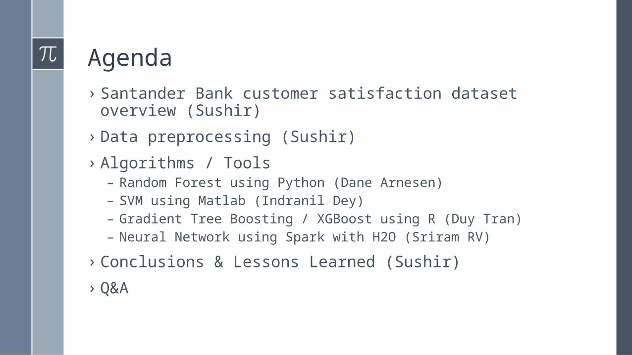
Agenda› Santander Bank customer satisfaction dataset overview

(Sushir)› Data preprocessing (Sushir)› Algorithms / Tools

– Random Forest using Python (Dane Arnesen)– SVM using Matlab (Indranil Dey)– Gradient Tree Boosting / XGBoost using R (Duy Tran)– Neural Network using Spark with H2O (Sriram RV)

› Conclusions & Lessons Learned (Sushir)› Q&A

Santander Bank Challenge• The competition was listed in www.kaggle.com.• Santander Bank wants to identify the dissatisfied

customers.• This will help them to take actions to improve the

customers happiness.• Which customers are unhappy?

– Happy = 0, Unhappy = 1– 371 features including CustomerID & TargetAttr– 76,020 rows in training data, only 3,008 rows where TargetAttr=1

Preprocessing Issues: More happy customer than unhappy customer. Variables were provided in Spanish so we don’t understand

the meaning of these variables. Data processing • How to remove highly correlated variables and zero

frequency variables Solution• Removal of zero variance attributes• Removal of highly correlated attributes using correlation

matrix

Random ForestPython

Python RandomForestClassifier› Python DS library called Scikit-Learn

– Classification, Regression, Clustering, Dimensionality Reduction, Visualization, etc.– Open Source– Recommend Anacanda download: https://www.continuum.io/downloads

› RandomForestClassifier part of the Ensemble family of classifiers– Using random subset of features + bagging techniques– Lots of parameters…

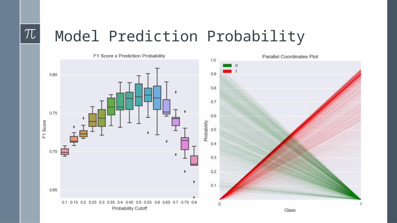
Model Prediction Probability

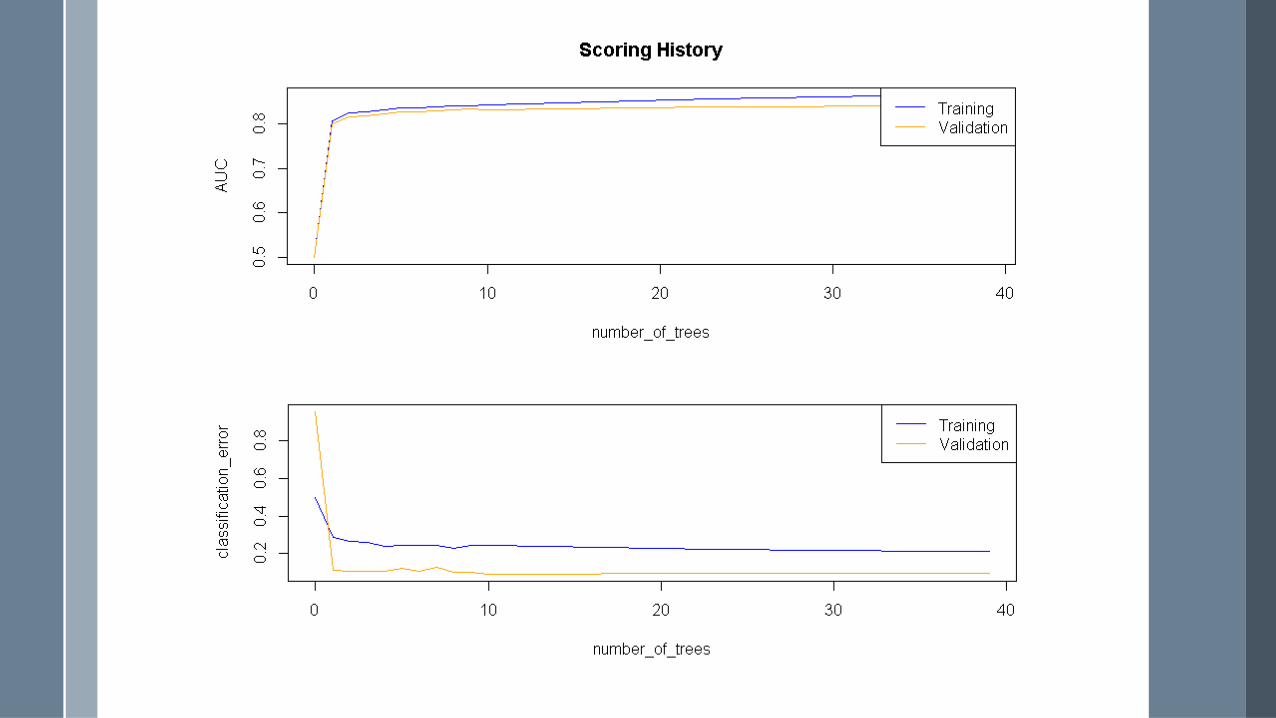
Number of Random Trees

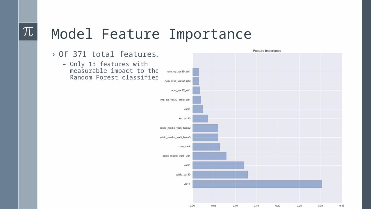
Model Feature Importance› Of 371 total features…

– Only 13 features with measurable impact to the Random Forest classifier

AUC Curve & Confusion MatrixClass 1 1 01 1603 (TP) 405 (FN)0 586 (FP) 1408 (TN)

› Using 55% probability cutoff:– Accuracy: 75%– TPR: 80%– FPR: 29%– Precision: 73%– F1: 76%

Support Vector MachineMatlab

12

Support Vector Machine › A Support Vector Machine (SVM) is a discriminative classifier formally

defined by a separating hyperplane. Given labeled training data (supervised learning), the algorithm outputs an optimal hyperplane which categorizes new examples.

Advantages:› SVMs produces large margin separating hyperplane, and efficient in higher dimension› It maximizes the margin between points closest to the boundary› SVMs only consider points near the margin (support vectors) – more robust

Disadvantages:› Due to complexity of the algorithm it requires high amount of memory and takes long time

to train the model and predict the test data› The model is sensitive to optimal choice of kernel and regularization parameters

13

Support Vector Machine MODEL INFO:Status: TrainedTraining Time: 04:48:27

Classifier Options Type: SVM Kernel function: Linear kernel scale: 1.0 Kernel scale mode: Auto Box constraint level: 1.0 Multiclass method: One-vs-One Standardize data: true Cross Validation: 10 Folds

Feature Selection Options  Features Included: 369

Validation Results Validation accuracy: 96%

› Model 1 : SVM using Linear Kernel – complete dataset with 369 predictors

Class Precision

Recall F1

0 100% 96.04% 97.98%1 0% 0% --

Class 0

AUC: 58.01%

Class 1

AUC: 58.01%

14

Reducing the Number of Predictors › By using MATLAB we created a correlation matrix for 369 predictors› From the correlation matrix we identified predictors which are highly

positively or negatively correlated– Highly positively correlated: Correlation greater than 0.75– Highly negatively correlated: Correlation less than -0.75

› After removing the highly correlated predictors the total number of predictors gor reduced to 115 from 369

Correlation Matrix with 369 Predictors

15

Balancing the Dataset & Applying PCA› After removal of correlated predictors the SVM models became more

trained in predicting class 0, which was not a desired outcome› To overcome this issue we had to balance the training dataset, i.e.

keeping equal number of records of both the classes in the training data– Using MATLAB randomly selected 3008 records of class 0 and combined 3008 records of

class 1

› Also to improve the SVM models further, we used PCA with 50 components– Principal component analysis (PCA) is a statistical procedure that uses an orthogonal

transformation to convert a set of observations of possibly correlated variables into a set of values of linearly uncorrelated variables called principal components#.

16

Support Vector Machine MODEL INFO:Status: TrainedTraining Time: 00:06:42

Classifier Options Type: SVM Kernel function: Linear kernel scale: 1 Kernel scale mode: Auto Box constraint level: 1.0 Multiclass method: One-vs-One Standardize data: true Cross Validation: 10 Folds

Feature Selection Options  Features Included: 115

PCA Options Enable PCA: true Maximum number of components: 50

Validation Results Validation accuracy: 72.6%

› Model 6 : SVM using Linear kernel – PCA (50 components)

Class Precision

Recall F1

0 72.47% 72.67% 72.57%1 72.74% 72.55% 72.64%

Class 0

AUC: 77.54%

Class 1

AUC: 77.54%

PCA explained variances: 61.5%, 28.6%, 10.0%, …….

17

Comparing the SVM Models› The model 6 has best prediction accuracy for both the classes

Model No.

Description Accuracy

Class Precision

Recall F1 AUC

Model 1 SVM Linear Kernel – Complete dataset with 369 predictors 96%

0 100% 96.04% 97.98%58.01%

1 0% 0% --

Model 2 SVM Linear Kernel – Complete dataset with 115 predictors 96%

0 99.99% 96.04% 97.98%59.68%

1 0% 0% --

Model 3SVM Gaussian Kernel – Complete dataset with 115 predictors

96%0 99.99% 96.04% 97.98%

51.07%1 0% 0% --

Model 4 SVM Linear Kernel – Balanced dataset with 115 predictors 70.8%

0 67.75% 72.14% 69.88%78.64%

1 73.84% 69.6% 71.66%

Model 5SVM Gaussian Kernel – Balanced dataset with 115 predictors

70.2%0 84.48% 65.71% 73.92%

77.58%1 55.92% 78.27% 65.23%

Model 6SVM Linear Kernel (PCA) – Balanced dataset with 115 predictors

72.6%0 72.47% 72.67% 72.57%

77.54%1 72.74% 72.55% 72.64%

* All models built with 10 folds cross-validation

18

Learnings from building SVM Model› Removing highly correlated predictors simplifies models› PCA is also a good way to deal with correlated attributes in a dataset› Unbalanced training dataset will impact the model’s prediction, and skew

it towards the class with higher number of instances in the dataset› There is no single way for increasing the prediction accuracy of a model,

we should take multiple approaches to iteratively improve the prediction accuracy of the predictive models

Gradient Tree BoostingR

Performance Metrics - GBMClass 1 Class 0

Class 1 256 316

Class 0 1104 13569

› Accuracy : 0.9069› Precision : 0.44755› TPR : 0.18824› TNR: 0.97724› F1 : 0.51751

Training Process - GBMNumber of TreesUse all observations?Use all predictors?Maximum depth of each treeLearning rateBalance response classes? Increase true positive rate but also increase false positive rate!

Hyperparameter optimization – Grid vs Random

http://h2o-release.s3.amazonaws.com/h2o/rel-turchin/3/docs-website/h2o-docs/booklets/GBM_Vignette.pdf

› Grid search – exhaustive, curse of dimensionality.

› Random search – found to be more effective: http://jmlr.csail.mit.edu/papers/volume13/bergstra12a/bergstra12a.pdf

› Easy parallelization

Neural NetworkSpark with H2O

What is Deep Learning?› Deep Learning learns a hierarchy of non linear transformations.› Neurons transform their input in non linear way.› Three types of neurons Input, Output and Hidden neurons› Input neurons get activated by numbers in your dataset and output neurons is

the output you want to see.

Why did I choose this model?• Prediction speed is fast and also the results are very significant with less

misclassification errors compared to any other algorithms. • Handles lots of irrelevant features well (separates signal from noise). • Automatically learns feature interactions.• H2O is a Java Virtual Machine that brings database-like interactiveness to

Hadoop that is optimized for doing “in memory” processing of distributed, parallel machine learning algorithms on clusters. It can be installed as a standalone or on top of existing Hadoop installation.

Performance Metrics – Deep LearningClass 0 Class 1

Class 0 64856 8156

Class 1 1673 1335

› Error Rate:0.12925› Accuracy: 0.70785› F1 : 0.31751

0.129295

Performance Metrics

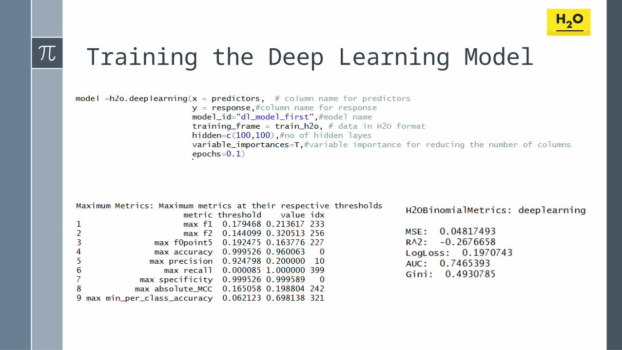
Training the Deep Learning Model

Spark Integration RStudio

Drawbacks› Needs a large data set.› The training time is long.› Needs a lot of parameter tuning (feature selection).› Features need to be on the same scale.

Conclusions & Lessons Learned

Conclusions & Lessons Learned› Understanding the concept of data mining using

Classification› Python/R/Scala/Matlab are useful tool for data mining› Data processing and removal of highly correlated

variables helps to identify the main variables.› Random Forest classifier/Confusion matrix

/PCA/SVM/Neural Network/ Gradient Tree Boosting› Combination of various technique helps to identify the

factors related to unsatisfied customers.› ROC curve was helpful to detect the accuracy of the

model.› Gradient Tree Boosting gave us the best model.

Q&A