bunker consumption optimization in liner shipping a metaheuristic approach

7/17/2019 Bunker Consumption Optimization in Liner Shipping a Metaheuristic Approach

http://slidepdf.com/reader/full/bunker-consumption-optimization-in-liner-shipping-a-metaheuristic-approach 1/11

International Journal on Recent and Innovation Trends in Computing and Communication ISSN: 2321-8169Volume: 3 Issue: 6 3766 - 3776

_______________________________________________________________________________________________

3766IJRITCC | June 2015, Available @ http://www.ijritcc.org

_______________________________________________________________________________________

Bunker Consumption Optimization in Liner Shipping: A Metaheuristic

Approach

Maxim A. Dulebenets

Department of Civil Engineering and Intermodal Freight Transportation InstituteThe University of Memphis

Memphis TN, USAE-mail: [email protected]

Abstract -Taking into account increasing volumes of the international seaborne trade, liner shipping companies have to ensureefficiency of their operations in order to remain competitive. The bunker consumption cost constitutes a substantial portion of thetotal vessel operating cost and directly affects revenues of liner shipping companies. “Slow steaming” became a common strategy

among ocean carriers to decrease vessel sailing speeds and reduce bunker consumption costs. However, decreasing vessel sailingspeeds may require deployment of more vessels on a given shipping route to provide the agreed service frequency at each port ofcall. Several bunker consumption optimization methods were developed in the past to capture those conflicting decisions. This

paper describes existing bunker consumption optimization methods, outlines their drawbacks, and proposes a new metaheuristicapproach. Numerical experiments demonstrate efficiency of the suggested metaheuristic in terms of solution quality and

computational time.Keywords- Maritime Transportation, Liner Shipping, Bunker Consumption Optimization, Metaheuristics

__________________________________________________*****_________________________________________________

I. I NTRODUCTION

The volume of cargo, carried by vessels, significantlyincreased over the last decades. According to InternationalChamber of Shipping [1], seaborne trade volumes havequadrupled over the last four decades and increased from8,000 billion ton-miles in 1968 to 32,000 billion ton-miles in2008. The heavy fuel oil (HFO) currently costs around $600

per ton, but is forecasted to increase up to $1,000 by 2020 [2].Furthermore, International Maritime Organization (IMO)regulations set a new limit for sulphur oxides (SOx) content inthe fuel outside the emission control areas from 4.50% m/m

before January 1, 2012 to 3.50% after January 1, 2012, fallingto 0.50% after January 1, 2020 [3]. Such drastic changes in thefuel chemical content requirements will force liner shippingcompanies to switch from HFO to more expensive marine gasoil (MGO). Currently MGO costs around $960 per ton, but is

projected to increase to $1,800 by 2020 and to $2,300 by 2035[2].

In order to improve transport efficiency liner shippingcompanies are slowing down their vessels, leading to

significant bunker consumption cost savings that maycomprise up to 75% of total vessel operational costs [4].Psaraftis and Kontovas [5] indicate that “slow steaming”,when a vessel sails at lower than the designed speed, became acommon strategy among liner shipping companies to reduce

bunker consumption costs. According to COSCO’s first half

year earnings statement, “slow steaming” reduced bunkerconsumption expenses by 18% in the first half of the year2014 [6]. However, “off-schedule ships, particularly the mega-

ships that are slow sailing to save costs, are also a

factor…causing port congestion” [7]. Drewry MaritimeResearch underlined that Asia-Europe route was the leastreliable during August-October 2014 with only 58% of vessels

arriving within the allocated time window (TW), which isconsidered as unacceptable for many shippers [8].

Several bunker consumption optimization (BCO) methodswere proposed in the literature to assist liner shippingcompanies in designing efficient vessel schedules. This paper

provides an overview of the existing approaches and suggestsa new metaheuristic approach. The rest of the paper isorganized as follows. The next section provides the problemdescription, while the third section presents the mathematicalformulation. The forth section overviews the existing BCOmethods to solve the considered problem and outlinesdrawbacks of those methods, while the fifth section describesthe developed metaheuristic. The sixth section discussesnumerical experiments that were performed in this study,while the last section provides conclusions and future researchavenues.

II. PROBLEM DESCRIPTION

The problem of vessel routing and scheduling in linershipping received a lot of attention from researchers and

practitioners, especially during the last ten years. For anexcellent review of strategic, tactical and operational decision

problems in liner shipping this study refers to Meng et al. [9].

This paper focuses on the vessel schedule design problem,described next.

A. Liner Shipping Route

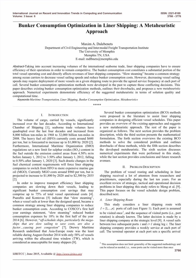
This study considers a liner shipping route with

},...,1{ n I ports of call (see Figure 1). Each port is assumed

to be visited once1, and the sequence of visited ports (i.e., port

rotation) is already known. The latter decision is made by aliner shipping company at the strategic level [9]. A vessel sails

between two subsequent ports i and i+1 along leg i. The linershipping company provides a weekly service at each port ofcall. The terminal operator at each port sets a specific arrival

1 This assumption does not limit generality of the suggested methodology and

can be relaxed as needed, i.e., some ports can be visited more than once

http://www.ijritcc.org/







_______________________________________________________________________________________________


_______________________________________________________________________________________

TW [ eitw – the earliest start at port i, l itw – the latest start at

port i], during which a vessel should arrive at the port (can beup to 1-3 days depending on the port). Weekly demand(TEUs) at each port is known, while the quantity of containerstransported by alliance partners is excluded from the totalweekly demand, as this decision is usually made by the liner

shipping company at the strategic level [9].

Figure 1. Illustration of a Shipping Route.

B. Vessel Service at Ports of Call

Terminal operators have various contractual agreementswith the liner shipping company, according to which eachterminal operator offers a set of handling rates

I i sS ii },...,1{ to the liner shipping company. If faster

service is requested, the port handling time for a given vesseldecreases, but the port handling charges, imposed to the linershipping company, increase. Note that reduced handling timeat a port may result in bunker consumption cost savings, sincea vessel can sail at a lower speed to the next port of call.

C. Vessel Arrivals

The following scenarios of vessel arrivals will be modeledin this study:

1) If a vessel arrives within a set arrival TW, no penaltieswill be imposed to the liner shipping company.

2) In certain cases a vessel departing from port i may arrive

at the next port i+1 before the earliest start eitw 1 , even when

sailing at the lowest possible speed minv . In such cases it is

assumed that the vessel will wait at a dedicated area at port i toensure arrival within the allocated TW at port i+1

2. The port

waiting time iwt can be estimated as d i

i

ieii t

v

l twwt 1 ,

where iv is the sailing speed on leg i, il is length of leg i, d it

is departure time from port i.

3) If a vessel arrives after the end of the latest start l itw 1 ,

monetary penalties are imposed to the liner shipping company(in USD/hr.), but the vessel will still start service uponarrival

3. The penalty value is assumed to linearly increase with

late arrival hours 1ilt .

2

Technically the vessel can also wait at port i+1, or split waiting times between ports i and i+1 3 It is assumed that the liner shipping company under consideration cannegotiate such an agreement

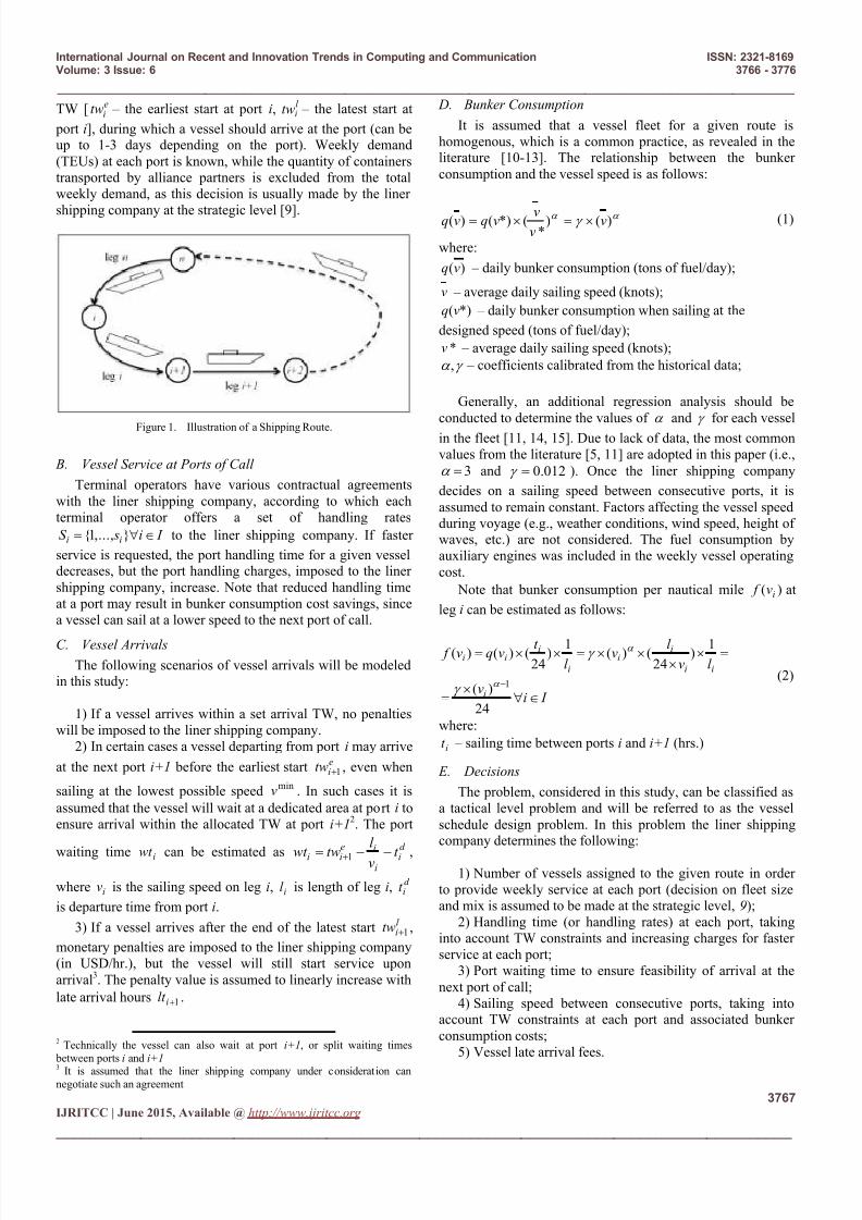
D. Bunker Consumption

It is assumed that a vessel fleet for a given route ishomogenous, which is a common practice, as revealed in theliterature [10-13]. The relationship between the bunkerconsumption and the vessel speed is as follows:

)()

*(*)()( v

v

vvqvq (1)

where:

)(vq – daily bunker consumption (tons of fuel/day);

v – average daily sailing speed (knots);

*)(vq – daily bunker consumption when sailing at the

designed speed (tons of fuel/day);

*v – average daily sailing speed (knots);

, – coefficients calibrated from the historical data;

Generally, an additional regression analysis should be

conducted to determine the values of and for each vesselin the fleet [11, 14, 15]. Due to lack of data, the most commonvalues from the literature [5, 11] are adopted in this paper (i.e.,

3 and 012.0 ). Once the liner shipping company

decides on a sailing speed between consecutive ports, it isassumed to remain constant. Factors affecting the vessel speedduring voyage (e.g., weather conditions, wind speed, height ofwaves, etc.) are not considered. The fuel consumption byauxiliary engines was included in the weekly vessel operatingcost.

Note that bunker consumption per nautical mile )( iv f at

leg i can be estimated as follows:

I iv

l v

l v

l

t vqv f

i

ii

ii

i

iii

24

)(

1)

24()(

1)

24()()(

1

(2)

where:

it – sailing time between ports i and i+1 (hrs.)

E. Decisions

The problem, considered in this study, can be classified asa tactical level problem and will be referred to as the vesselschedule design problem. In this problem the liner shipping

company determines the following:

1) Number of vessels assigned to the given route in orderto provide weekly service at each port (decision on fleet sizeand mix is assumed to be made at the strategic level, 9);

2) Handling time (or handling rates) at each port, takinginto account TW constraints and increasing charges for fasterservice at each port;

3) Port waiting time to ensure feasibility of arrival at thenext port of call;

4) Sailing speed between consecutive ports, taking intoaccount TW constraints at each port and associated bunkerconsumption costs;

5)

Vessel late arrival fees.









_______________________________________________________________________________________________


_______________________________________________________________________________________

A liner shipping company sets a maximum quantity of

vessels that can be deployed at any given route ( maxqq ) and

sets limits on lower and upper vessel sailing speed

( I ivvv i maxmin ). The minimum sailing speed minv is

selected to reduce wear of the vessel’s engine [16], while the

maximum sailing speedmax

v is defined by the capacity of thevessel’s engine [5]. Note that all decisions are interrelated.Selecting lower sailing speed reduces bunker consumption, butmay require deployment of more vessels at the given route toensure that weekly service is met, which increases the totalweekly operating cost (e.g., crew costs, maintenance, repairs,insurance, etc.). Various port handling rates further allow theliner shipping company to weigh different options betweensailing and port handling times (e.g., faster handling ratereduces the service time at a given port, which may allowsailing at a lower speed to the next port of call). On the otherhand, higher handling rates may not always be favorable asthey may lead to the vessel waiting once service is completed.

III.

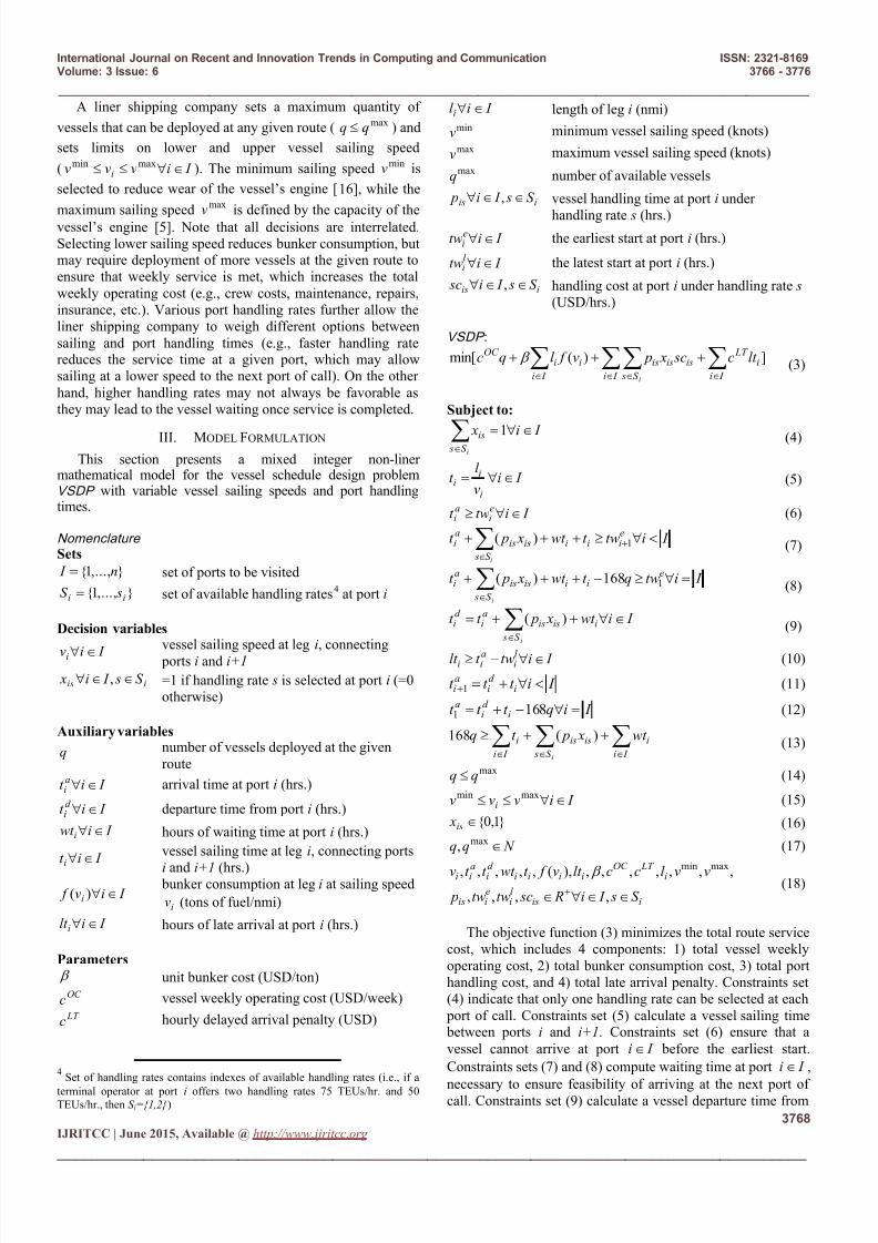
MODEL FORMULATION

This section presents a mixed integer non-linermathematical model for the vessel schedule design problemVSDP with variable vessel sailing speeds and port handlingtimes.

Nomenclature

Sets

},...,1{ n I set of ports to be visited

},...,1{ ii sS set of available handling rates4 at port i

Decision variables

I ivi vessel sailing speed at leg i, connecting ports i and i+1

iis S s I i x ,

=1 if handling rate s is selected at port i (=0otherwise)

Auxiliary variables

q number of vessels deployed at the givenroute

I it ai arrival time at port i (hrs.)

I it d i departure time from port i (hrs.)

I iwt i hours of waiting time at port i (hrs.)

I it i vessel sailing time at leg i, connecting portsi and i+1 (hrs.)

I iv f i )( bunker consumption at leg i at sailing speed

iv (tons of fuel/nmi)

I ilt i hours of late arrival at port i (hrs.)

Parameters unit bunker cost (USD/ton)OC c vessel weekly operating cost (USD/week) LT c hourly delayed arrival penalty (USD)

4 Set of handling rates contains indexes of available handling rates (i.e., if a

terminal operator at port i offers two handling rates 75 TEUs/hr. and 50TEUs/hr., then S i={1,2})

I il i length of leg i (nmi)

minv

minimum vessel sailing speed (knots)maxv

maximum vessel sailing speed (knots)max

q

number of available vessels

iis S s I i p ,

vessel handling time at port i under

handling rate s (hrs.)

I itwei the earliest start at port i (hrs.)

I itwl i the latest start at port i (hrs.)

iis S s I i sc ,

handling cost at port i under handling rate s (USD/hrs.)

VSDP :

])(min[ i

I i

LT

I i S s

isisisi

I i

iOC lt c sc x pv f l qc

i

(3)

Subject to:

iS s

is I i x 1 (4)

I iv

l t

i

ii (5)

I itwt e

iai (6)

iS s

eiiiisis

ai I itwt wt x pt 1)(

(7)

iS s

eiiisis

ai I itwqt wt x pt 1168)(

(8)

I iwt x pt t

iS s

iisisai

d i

)( (9)

I itwt lt l i

aii

(10)

I it t t id i

ai 1 (11)

I iqt t t id i

a 1681 (12)

iS s I i

iisis

I i

i wt x pt q )(168

(13)

maxqq (14)

I ivvv i maxmin

(15)

}1,0{is x (16)

N qq max

, (17)

iisl i

eiis

i LT OC

iiiid i

aii

S s I i R sctwtw p

vvl cclt v f t wt t t v

,,,,

,,,,,,,),(,,,,, maxmin (18)

The objective function (3) minimizes the total route servicecost, which includes 4 components: 1) total vessel weeklyoperating cost, 2) total bunker consumption cost, 3) total porthandling cost, and 4) total late arrival penalty. Constraints set(4) indicate that only one handling rate can be selected at each

port of call. Constraints set (5) calculate a vessel sailing time between ports i and i+1. Constraints set (6) ensure that a

vessel cannot arrive at port I i before the earliest start.

Constraints sets (7) and (8) compute waiting time at port I i ,necessary to ensure feasibility of arriving at the next port ofcall. Constraints set (9) calculate a vessel departure time from








_______________________________________________________________________________________________


_______________________________________________________________________________________

port I i . Constraints set (10) estimate hours of late arrival at

port I i . Constraints sets (11) and (12) compute a vessel

arrival at the next port of call I i )1( . Constraints set (13)

ensure weekly service frequency (168 denotes the totalnumber of hours in a week). The right-hand-side of an equalityestimates the total turnaround time of a vessel at the given

route (where the first component is the total sailing time, thesecond component is the total port handling time, and the thirdcomponent is the total port waiting time). Constraints set (14)ensure that the number of vessels to be deployed at the givenroute should not exceed the number of available vessels.Constraints set (15) show that a vessel sailing speed should bewithin specific limits. Constraints (16) – (18) define ranges of

parameters and variables.

IV. STATE OF THE ART

One of the difficulties in solving tactical level problems inliner shipping is non-linearity of the bunker consumption

function (the second component of the VSDP objective). Thereexist several methods to address this issue:

1) Enumeration Method (M1) – it is assumed that sailingspeed remains constant throughout the voyage, i.e. does notchange from leg to leg [17, 18]. In this case the required sailingspeed can be determined based on the number of vesselsdeployed at the given route, the total port handling and waitingtimes, and required frequency of service (using eq. (13) inVSDP ). The total cost (estimated as a sum of bunkerconsumption and operating costs) should be computed for all

possible scenarios by varying the number of deployed vessels(typically does not exceed 20-25), and then the best alternativeshould be selected (see Figure 2A).

Figure 2. Existing BCO Methods.

2)

Dynamic Programming Method (M2) – requiresconstruction of a time-space network, where the x-axisrepresents ports to be visited (see Figure 2B) and y-axisrepresents time, discretized in days. Once the time-spacenetwork is created, the problem of selecting vessel speed andquantity of deployed vessels can be reduced to the shortest path

problem [19, 20].

3) Discretization Method (M3) – vessel sailing speed

reciprocali

iv

y 1 is discretized (see Figure 2C), and the

bunker consumption )( i yG is estimated for each value of i y

[15, 21].

4)

Tailored Methods (M4) – a linear or quadraticapproximation is used for the non-linear bunker consumption

function [11, 12, 16]. The linear approximation can berepresented either by a set of tangent (see Figure 2D) or secantlines (see Figure 2E). The quadratic approximation can berepresented by a set of parabolas (see Figure 2F).Approximations can be static or dynamic. Staticapproximations have a predetermined number of elements(either lines or parabolas). Dynamic approximations requiregenerating additional elements if after solving linear orquadratic VSDP the approximation error ε exceeds a targetlimit.

5) Second Order Conic Programming (SOCP) Method (M5) – requires transformation of the original VSDP formulation tothe SCOP formulation [14].

For a detailed review of BCO methods this study refers toWang et al. [16]. Drawbacks of the existing methods can besummarized as follows:








_______________________________________________________________________________________________


_______________________________________________________________________________________

1) In reality it is highly unlikely that a vessel will sail at thesame speed throughout the whole voyage as assumed by M1.The vessel may be required to wait at the given port of call fora significant amount of time in order to arrive at the next portof call within the allocated TW.

2) Higher time discretization rate (e.g., discretize every 4hrs. instead of discretizing every day, see Figure 2B) will

increase the number of nodes in the time-space network, whichin turn will increase the computational time of M2.Furthermore, the optimal solution, which lies between twonodes (e.g., 8.7 hrs. lying between 8 hrs. and 12 hrs. in case of4 hrs. discretization rate), will never be discovered.

3) Similar to M2, higher speed discretization rate willincrease the computational time of M3.

4) All tailored methods have an approximation error ε. Theerror can be reduced by increasing number of elements in theapproximation. Dynamic approximations require solvinglinearized or quadratic VSDP more than once.

5) M5 requires a mixed integer SOCP solver for VSDP withSOCP constraints.

V.

SOLUTION APPROACH

A Memetic Algorithm (MA) was developed to addressdrawbacks of the existing BCO methods, described in the

previous section. MAs belong to the group of EvolutionaryAlgorithms (EAs ), and are widely used for solving complex

problems in different fields [22]. However, while EAs construct individuals using stochastic operators, MAs employalong with the stochastic operators local search heuristics andgenerally provide higher quality solutions and fasterconvergence [22]. Advantages of the proposed MA to existingBCO methods are as follows:

1) Does not restrict the vessel sailing speed to remainconstant throughout the voyage (unlike M1);

2) Considers the entire search space (unlike M2 and M3,which discretize the search space);

3) Estimates bunker consumption using the non-linearfunction without generating approximations, which have acertain error ε (unlike M4);

4)

Does not require any specific solvers and transformationof VSDP formulation (unlike M5);

The main steps of the developed MA are outlined inProcedure 1. In steps 1- 4 the chromosomes and population areinitialized. In step 5 fitness of the initial population isevaluated. Then, the algorithm enters the main loop (steps 7

through 11). In step 8, function )( gen Popnts SelectPare

identifies parents from the current population (i.e., variable

gen Parents ) to be used in step 9 and produce new offspring. In

step 9, function ),( MutRate Parents genn MAoperatio applies a

custom operator, which uses a stochastic search and a localsearch heuristic (LSH ) to produce new offspring (i.e., variable

genOffspring ). In step 10, function )( genOffspring Evaluate

calculates fitness function values (i.e., variable gen Fit ) for the

offspring, and in step 11, function

),( gen gen Fit Offspring Select selects individuals, based on

their fitness, to become candidate parents in the nextgeneration. MA exits the loop, when a termination criterion issatisfied. The algorithm was coded in MATLAB R2014a.

Next this section presents in detail each of the components ofthe developed MA.

Procedure 1. Memetic Algorithm),,,,( ionStopCriter MutRate PopSizeS I iMA

in: },...,1{ n I - set of ports to be visited; },...,1{ ii sS - set of available rates at each port; PopSize - population size;

MutRate - mutation rate; ionStopCriter - stopping criterion

out: BestChrom - the best vessel schedule

1: ;;;; PopSizeOffspring PopSize Parents PopSize Fit PopSize Pop ⊲ Initialization

2: ),( iS I Chrom InitChrom ⊲ Chromosome initialization

3: 0 gen

4: ),( PopSizeChrom Pop gen InitPop ⊲ Population initialization

5: )( gen gen Pop Fit Evaluate ⊲

Initial population fitness evaluation

6: while FALSE iterionStoppingCr do

7: 1 gen gen

8: )( gen gen Pop Parents nts SelectPare ⊲ Select parents

9: ),( MutRate ParentsOffspring gen gen n MAoperatio ⊲ Produce offspring

10: )( gen gen Offspring Fit Evaluate ⊲ Offspring fitness evaluation

11: ),(1 gen gen gen Fit Offspring Pop Select ⊲ Define population in the next generation

12: end while

13: return BestChrom








_______________________________________________________________________________________________


_______________________________________________________________________________________

A. Chromosome Representation

A real valued chromosome was used in the developed MA to represent a solution (i.e., vessel schedule). An example of achromosome is presented in Figure 3 for a liner shipping routewith 8 ports of call. For each port the chromosome includesthe following information: a) arrival time, b) sailing speed to

the next port, c) handling rate selected, and d) waiting time.For example, according to the schedule the vessel shouldarrive at the 3rd port of call on Thursday at 2:42 PM (i.e.,3×24+14.7=86.7 hrs.), be served at the port under handlingrate of 100 TEUs/hr., wait for 14.7 hrs. after servicecompletion, and sail to the next port of call at the speed of 24.0knots.

Figure 3. Chromosome Representation.

B. Chromosome and Population Initialization

Two LSHs are used to initialize the population. The firstLSH is directed to minimize the total number of deployedvessels at the given route by selecting the maximum handlingrate (i.e., minimum port time) at each port of call and themaximum possible sailing speed between ports, taking into

account TW constraints. The first LSH will be referred to asMinimizing the Number of Deployed Vessels Heuristic(MINDVH ). The second LSH is directed to maximize the totalnumber of deployed vessels at the given route by selecting theminimum handling rate (i.e., maximum port time) at each portof call and the minimum possible sailing speed between ports,taking into account TW constraints. The second LSH will bereferred to as Maximizing the Number of Deployed VesselsHeuristic (MANDVH ). LSHs are outlined in Procedures 2 and3.

Procedure 2. Minimizing the Number of Deployed Vessels Heuristic

),,,,,,( min

isl i

eiii pvtwtwl S I MINDVH

in: },...,1{ n I - set of ports to be visited; },...,1{ ii sS - set of available rates at each port; il - length of leg i; eitw - the

earliest start at port i; l itw - the latest start at port i; minv - minimum sailing speed; is p - vessel handling time at port i under


out:at - arrival time at each port of call; v - vessel sailing speed; p - handling time at each port of call; wt - waiting time at

each port of call;

1: nwt n pnvnt a ;;; ⊲ Initialization

2: ea twt i 11;1

3: for all I i do

4: )min( isi p p ⊲ Select handling time

5: if min

1 )(v

pt tw

l

iai

l i

i

then

6: )(min1 i

ai

il ii pt

v

l twwt ⊲ Estimate waiting time

7: else

8: 0iwt

9: end if

10:)(1 ii

ai

l i

ii

wt pt twl v

⊲

Estimate vessel sailing speed

11:i

iii

ai

ai

v

l wt pt t 1 ⊲ Estimate arrival time at the next port of call

14: 1 ii

15: end for

16: return wt pvt a

,,,

Half of the population will be initialized using MINDVH ,while the other half will be initialized using MANDVH .Preliminary MA runs were performed to select the population

size PopSize, and results will be presented in the numericalexperiments section.

C. Parent Selection

Parent selection determines individuals from the current

population that will be allowed to produce offspring via MA operations at a given generation. The proposed MA applies a








_______________________________________________________________________________________________


_______________________________________________________________________________________

deterministic parent selection scheme (i.e., all survivedoffspring become parents), as this strategy is widely used inEvolutionary Programming and Genetic Algorithms [22].

Procedure 3. Maximizing the Number of Deployed Vessels Heuristic

),,,,,,( minis

l i

eiii pvtwtwl S I MANDVH

in: },...,1{ n I - set of ports to be visited; },...,1{ ii sS - set of available rates at each port; il - length of leg i; eitw – the

earliest start at port i; l itw – the latest start at port i; minv - minimum sailing speed; is p - vessel handling time at port i under


out:at - arrival time at each port of call; v - vessel sailing speed; p - handling time at each port of call; wt - waiting time at

each port of call;

1: nwt n pnvnt a

;;; ⊲ Initialization

2: ea twt i 11;1

3: for all I i do

4: )max( isi p p ⊲ Select handling time

5: if min

1 )(v

pt twl

iai

l i

i

then

6: )(min1 i

ai

il ii pt

v

l twwt ⊲

Estimate waiting time

7: else

8: 0iwt

9: end if

10:)(1 ii

ai

l i

ii

wt pt tw

l v

⊲ Estimate vessel sailing speed

11:i

iii

ai

ai

v

l wt pt t 1 ⊲ Estimate arrival time at the next port of call

14: 1 ii

15: end for

16: return wt pvt a

,,,

D. MA Operations

A custom MA operator was developed in this study to produce offspring. The MA operation will be performed forrandomly selected ports of call, belonging to the given shippingroute (stochastic search). The mutation rate MutRate definesthe number of ports, which will undergo the MA operation. Forselected ports the MA operator will apply LSH . An example ofthe MA operation at port i is presented in Figure 3, where theMA operator performs the following steps:

1) Generate a number of candidate solutions Dd with i)arrival times, satisfying TW constraint at port i:

rand twtwtwt ei

l i

ei

aid )( , where rand is a random number

between 0 and 1, and ii) randomly selected port handling ratefrom the available handling rates at port i;

2) Flip the coin and get the value between 0 and 1;

3) If the coin value is zero, select new arrival time aid t and

handling rate ir , which minimize the bunker consumption cost

from sailing between ports i-1 and i+1 and the handling cost at port i (i.e., find the shortest path between ports i-1 and i+1);

Else, select new arrival time aid t and handling rate ir , which

maximize the bunker consumption cost from sailing between ports i-1 and i+1 and the handling cost at port i (i.e., find thelongest path between ports i-1 and i+1);

4) Update the chromosome based on new arrival time andhandling rate.

Figure 4. MA Operation.

Note that by selecting the shortest path between ports i-1 and i+1 the MA operator might increase the number of vessels








_______________________________________________________________________________________________


_______________________________________________________________________________________

to be deployed at the given route and vice versa. The number ofcandidate solutions, generated at each mutated port of call, will

be referred to as discretization rate DisRate . Preliminary MA

runs were performed to select MutRate and DisRate values,and results will be presented in the numerical experimentssection.

E.

Fitness FunctionFor EAs/MAs the fitness function is usually associated

with the objective function [22]. In the proposed MA thefitness function value was set equal to the objective functionvalue without applying any scaling mechanisms.

F. Offspring Selection

The offspring selection at a given generation of a MA is animportant part of its design [22]. The Tournament Selection isused in the developed MA. The Tournament Selection has two

parameters: a) tournament size ( TourSize ) – number of

individuals participating in each tournament, and b)

individuals selected ( IndSel ) – number of individuals selected

based on their fitness in each tournament to become candidate parents in the next generation. Preliminary MA runs were performed to select values of those parameters and results will be presented in the numerical experiments section. The ElitistStrategy [22] is applied in the developed MA to ensure that the

best individual lives more than one generation.

G. Stopping Criterion

In this paper the algorithm was terminated, if no change inthe objective function value was observed after a pre-specified

number of generations ( MaxNumGen of 300 generations) or

the maximum number of generations was reached

( LimitGen of 500 generations).

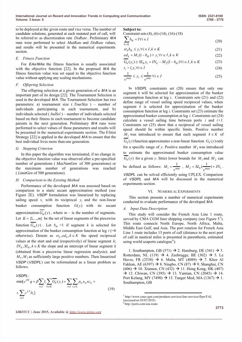
H. Comparison to the Existing Method

Performance of the developed MA was assessed based oncomparison to a static secant approximation method (seeFigure 2E). VSDP formulation was linearized by replacing

sailing speed iv with its reciprocal i y and the non-linear

bunker consumption function )( yG with its secant

approximation )( yGm , where m – is the number of segments.

Let },...,1{ m K be the set of linear segments of the piecewise

function )( yGm . Let ik b =1 if segment k is selected for

approximation of the bunker consumption function at leg i (=0

otherwise). Denote as K k ed st k k ,, the speed reciprocalvalues at the start and end (respectively) of linear segment k ;

K k SL IN k k ,, the slope and an intercept of linear segment k

(obtained from a piecewise linear regression analysis); and

21, M M as sufficiently large positive numbers. Then linearized

VSDP (VSDPL) can be reformulated as a linear problem asfollows.

VSDPL :

]

)(min[

i I i

LT

I i S s

isisis

K k

ik

I i

iOC

lt c

sc x p yGl qc

i

(19)

Subject to:Constraint sets (4), (6)-(14), (16)-(18)

K k

ik I ib 1 (20)

K k I i yb st iik k , (21)

K k I i yb M ed iik k ,)1(1 (22)

K k I ib M IN ySL yG ik k ik ik ,)1()( 2 (23)

I i yl t iii (24)

I iv

yv

i minmax

11 (25)

In VSDPL constraints set (20) ensure that only onesegment k will be selected for approximation of the bunkerconsumption function at leg i. Constraints sets (21) and (22)define range of vessel sailing speed reciprocal values, whensegment k is selected for approximation of the bunkerconsumption function at leg i. Constraints set (23) estimate the

approximated bunker consumption at leg i. Constraints set (24)calculate a vessel sailing time between ports i and i+1.

Constraints set (25) show that a reciprocal of vessel sailingspeed should be within specific limits. Positive number

1 M was introduced to ensure that each segment K k of

)( yGk function approximates a non-linear function )( yGk only

for a specific range of y. Positive number 2 M was introduced

to estimate the approximated bunker consumption value

)( yGk for a given y. Strict lower bounds for 1 M and 2 M can

be defined as follows:min1

1

v M , 1max2 )

1( IN

vSL M k .

VSDPL can be solved efficiently using CPLEX. Comparisonof VSDPL and MA will be discussed in the numericalexperiments section.

VI. NUMERICAL EXPERIMENTS

This section presents a number of numerical experimentsconducted to evaluate performance of the developed MA.

A. Input Data Description

This study will consider the French Asia Line 1 route,served by CMA CGM liner shipping company (see Figure 5

5).

This route connects North Europe, North Africa, Malta,Middle East Gulf, and Asia. The port rotation for French AsiaLine 1 route includes 15 ports of call (distance to the next portof call in nautical miles is presented in parenthesis, estimatedusing world seaports catalogue

6):

1. Southampton, GB (571) 2. Hamburg, DE (341) 3.Rotterdam, NL (119) 4. Zeebrugge, BE (302) 5. LeHavre, FR (2538) 6. Malta, MT (4089) 7. Khor AlFakkan, AE (6397) 8. Ningbo, CN (87) 9. Shanghai, CN(606) 10. Xiamen, CN (432) 11. Hong Kong, HK (407) 12. Chiwan, CN (395) 13. Yantian, CN (2045) 14.Port Kelang, MY (7490) 15. Tanger Med, MA (1367) 1.Southampton, GB

5 http://www.cma-cgm.com/products-services/line-services/flyer/FAL(accessed on 03/07/2015)6 http://ports.com/sea-route








_______________________________________________________________________________________________


_______________________________________________________________________________________

Figure 5. French Asia Line 1.

The required numerical data were generated based on theavailable liner shipping literature and are presented in Table 1.The latest start at each port of call was set using the following

relationship:];[

maxmin1vvU

l twtw il

il i , where U denotes

uniformly distributed pseudorandom numbers. The duration of

a TW ( ei

l i twtw ) was assigned as ]72;24[U hrs. [23]. A set of

available port handling times is p at each port of call was

assigned based on the weekly demand i NC (in TEUs) and the

available handling rates iS at the given port. Large ports were

assumed to have the weekly demand, uniformly distributed between 500 TEUs and 2000 TEUs. Note that term “large

port” was applied to those ports of call, if they were included

in the list of top 20 world container ports based on theirthroughput [24]. Weekly demand for smaller ports wasuniformly distributed between 200 TEUs and 1000 TEUs.Large ports were able to offer 4 possible handling rates: [125;100; 75; 50] TEUs/hr. Smaller ports could provide either 3([100; 75; 50] TEUs/hr.) or 2 handling rates ([75; 50]TEUs/hr.). The latter assumption can be explained by the factthat terminal operators at large ports usually have more vesselhandling equipment available and can offer more handling rateoptions to the liner shipping company. Furthermore, higher

amounts of TEUs handled can increase productivity.TABLE I. NUMERICAL DATA

Bunker consumption coefficients α,γ α=3,γ=0.012

Unit bunker cost β (USD/ton) 500

Vessel weekly operating cost cOC (USD/week) 300,000

Delayed arrival penalty c LT (USD/hr.) U[5,000; 10,000]

Minimum vessel sailing speed vmin (knots) 10

Maximum vessel sailing speed vmax (knots) 25

Maximum number of deployed vessels qmax 20

TW duration (hrs.) U[24; 72]

The handling cost at each port i under handling rate s was

computed as: iis S s I iU asc sc ,]50;0[ , where asc is

the average container handling cost. Based on the availableliterature [25-28] and assuming a mix of vessel operations thatinclude mooring, loading and discharge of containers, type of

container (empty, loaded, size, reefer), re-stowing (on-boardthe vessel or via quay), the average container handling costwas set equal to [700; 625; 550; 475] USD/TEU for handlingrates [125; 100; 75; 50] TEUs/hr. respectively. It was assumedthat each terminal operator perceives handling cost differently(i.e., service charge for the same handling rate varies from portto port), which is accounted for by the second (and random)

term of the is sc formula.

All numerical experiments were conducted on a DellT1500 Intel(T) Core i5 Processor with 1.96 GB of RAM. Astatic secant approximation for the bunker consumptionfunction was developed using MATLAB 2014a. A linearized

mixed-integer problem formulation VSDPL was solved usingCPLEX of General Algebraic Modeling System (GAMS).

B. MA Parameter Tuning

Based on preliminary MA runs the following values will beset for MA parameters: 1) PopSize = 40, 2) MutRate = 2, 3)

DisRate = 10, 4) TourSize = 15, and 5) IndSel = 10.

C. MA Performance

A total of 20 instances were developed using the data,described in the beginning of section VI and presented inTable 1, by changing arrival TW at each port of call. Thedeveloped MA was compared to VSDPL , which applies thestatic secant approximation with m=100 segments for the

bunker consumption function linearization. Results for all 20 problem instances are presented in Table 2, where columns 1through 8 show the following: 1) problem instance; 2) truevalue of the objective function Z at the optimal solution (i.e.,value of the non-linear objective function at the solution,

provided by VSDPL); 3) objective function value, provided byVSDPL ; 4) average over 10 replications objective function

value, provided by MA; 5) VSDPL gap Z

Z Z )(VSDPL ;

6) MA gap Z

Z Z )(MA ; 7) average over 10 replications

VSDPL computational time t(VSDPL); 8) average over 10

replications MA computational time t(MA).








_______________________________________________________________________________________________


_______________________________________________________________________________________

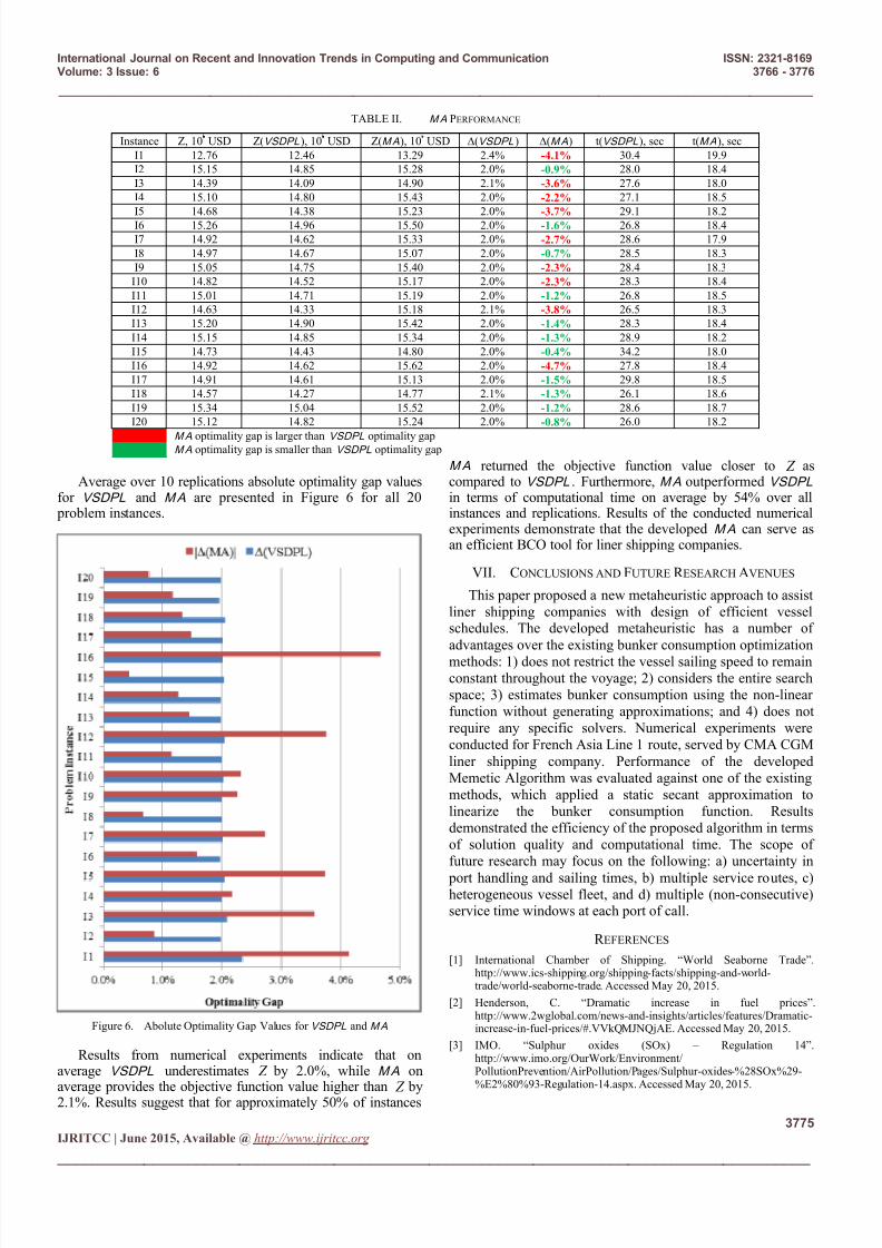
TABLE II. MA PERFORMANCE

Instance Z, 10 USD Z(VSDPL ), 10 USD Z(MA), 10 USD ∆(VSDPL ) ∆(MA) t(VSDPL), sec t(MA), sec

I1 12.76 12.46 13.29 2.4% -4.1% 30.4 19.9

I2 15.15 14.85 15.28 2.0% -0.9% 28.0 18.4

I3 14.39 14.09 14.90 2.1% -3.6% 27.6 18.0

I4 15.10 14.80 15.43 2.0% -2.2% 27.1 18.5

I5 14.68 14.38 15.23 2.0% -3.7% 29.1 18.2I6 15.26 14.96 15.50 2.0% -1.6% 26.8 18.4

I7 14.92 14.62 15.33 2.0% -2.7% 28.6 17.9

I8 14.97 14.67 15.07 2.0% -0.7% 28.5 18.3

I9 15.05 14.75 15.40 2.0% -2.3% 28.4 18.3

I10 14.82 14.52 15.17 2.0% -2.3% 28.3 18.4

I11 15.01 14.71 15.19 2.0% -1.2% 26.8 18.5

I12 14.63 14.33 15.18 2.1% -3.8% 26.5 18.3

I13 15.20 14.90 15.42 2.0% -1.4% 28.3 18.4

I14 15.15 14.85 15.34 2.0% -1.3% 28.9 18.2

I15 14.73 14.43 14.80 2.0% -0.4% 34.2 18.0

I16 14.92 14.62 15.62 2.0% -4.7% 27.8 18.4

I17 14.91 14.61 15.13 2.0% -1.5% 29.8 18.5

I18 14.57 14.27 14.77 2.1% -1.3% 26.1 18.6

I19 15.34 15.04 15.52 2.0% -1.2% 28.6 18.7

I20 15.12 14.82 15.24 2.0% -0.8% 26.0 18.2

MA optimality gap is larger than VSDPL optimality gapMA optimality gap is smaller than VSDPL optimality gap

Average over 10 replications absolute optimality gap valuesfor VSDPL and MA are presented in Figure 6 for all 20

problem instances.

Figure 6. Abolute Optimality Gap Values forVSDPL and MA

Results from numerical experiments indicate that on

average VSDPL underestimates Z by 2.0%, while MA onaverage provides the objective function value higher than Z by2.1%. Results suggest that for approximately 50% of instances

MA returned the objective function value closer to Z ascompared to VSDPL . Furthermore, MA outperformed VSDPL in terms of computational time on average by 54% over allinstances and replications. Results of the conducted numericalexperiments demonstrate that the developed MA can serve asan efficient BCO tool for liner shipping companies.

VII. CONCLUSIONS AND FUTURE R ESEARCH AVENUES

This paper proposed a new metaheuristic approach to assistliner shipping companies with design of efficient vesselschedules. The developed metaheuristic has a number of

advantages over the existing bunker consumption optimizationmethods: 1) does not restrict the vessel sailing speed to remainconstant throughout the voyage; 2) considers the entire searchspace; 3) estimates bunker consumption using the non-linearfunction without generating approximations; and 4) does notrequire any specific solvers. Numerical experiments wereconducted for French Asia Line 1 route, served by CMA CGMliner shipping company. Performance of the developedMemetic Algorithm was evaluated against one of the existingmethods, which applied a static secant approximation tolinearize the bunker consumption function. Resultsdemonstrated the efficiency of the proposed algorithm in termsof solution quality and computational time. The scope of

future research may focus on the following: a) uncertainty in port handling and sailing times, b) multiple service routes, c)heterogeneous vessel fleet, and d) multiple (non-consecutive)service time windows at each port of call.

R EFERENCES

[1] International Chamber of Shipping. “World Seaborne Trade” . http://www.ics-shipping.org/shipping-facts/shipping-and-world-trade/world-seaborne-trade. Accessed May 20, 2015.

[2] Henderson, C. “Dramatic increase in fuel prices”.http://www.2wglobal.com/news-and-insights/articles/features/Dramatic-increase-in-fuel-prices/#.VVkQMJNQjAE. Accessed May 20, 2015.

[3] IMO. “Sulphur oxides (SOx) – Regulation 14”.http://www.imo.org/OurWork/Environment/

PollutionPrevention/AirPollution/Pages/Sulphur-oxides-%28SOx%29-%E2%80%93-Regulation-14.aspx. Accessed May 20, 2015.








_______________________________________________________________________________________________


_______________________________________________________________________________________

[4] Ronen, D. “The effect of oil price on containership speed and fleet size”.Journal of the Operational Research Society, vol. 62, 2011, pp. 211-216.

[5] Psaraftis, H. and Kontovas, C. “Speed models for energy-efficientmaritime transportation: A taxonomy and survey”. TransportationResearch Part C, vol. 26, 2013, pp. 331 – 351.

[6] Cargo Business. “Cosco adds fuel-efficient ships to revive profits”.http://www.cargobusinessnews.com/news/092514/news2.html. AccessedMay 20, 2015a.

[7]

Cargo Business. “Drewry explores global port congestion”.http://www.cargobusinessnews.com/ news/093014/news1.html.Accessed May 20, 2015.

[8] Cargo Business. “Drewry: Maersk and Hamburg Süd are the top twomost reliable container carriers”.http://www.cargobusinessnews.com/news/techwire/Tech_Archives/121214/news.html. Accessed May 20, 2015.

[9] Meng, Q., Wang, S., Andersson, H., and Thun, K. “ContainershipRouting and Scheduling in Liner Shipping: Overview and FutureResearch Directions”. Transportation Science, vol. 48, 2014, pp. 265 -280.

[10] Wang, S. and Meng, Q. “Liner ship route schedule design with seacontingency time and port time uncertainty”. Transportation ResearchPart B, vol. 46, 2012, pp. 615 – 633.

[11] Wang, S. and Meng, Q. “Sailing speed optimization for container ships

in a liner shipping network”. Transportation Research Part E, vol. 48,2012, pp. 701 – 714.

[12] Wang, S. and Meng, Q. “Robust schedule design for liner shippingservices”. Transportation Research Part E, vol. 48, 2012, pp. 1093 – 1106.

[13] Wang, S., Meng, Q., and Liu, Z. “Containership scheduling with transit-time-sensitive container shipment demand”. Transportation ResearchPart B, vol. 54, 2013, pp. 68 – 83.

[14] Du, Y., Chen, Q., Quan, X., Long, L., and Fung, R. “Berth allocationconsidering fuel consumption and vessel emissions”. TransportationResearch Part E, vol. 47, 2011, pp. 1021 – 1037.

[15] Yao, Z., Ng, S., and Lee, L. “A study on bunker fuel management for theshipping liner services”. Computers and Operation Research, vol. 39,2012, pp. 1160-1172.

[16] Wang, S., Meng, Q., and Liu, Z. “Bunker consumption optimizationmethods in shipping: A critical review and extensions”. Transportation

Research Part C, vol. 53, 2013, pp. 49 – 62.

[17] Corbett, J, Wang, H., and Winebrake, J. “The effectiveness and costs ofspeed reductions on emissions from international shipping”.Transportation Research Part D, vol. 14, 2009, pp. 593 – 598.

[18] Ronen, D. “The effect of oil price on containership speed and fleet size”.Journal of the Operational Research Society, vol. 62, 2011, pp. 211 – 216.

[19] Fagerholt, K., Laporte, G., and Norstad, I. “Reducing fuel emissions byoptimizing speed on shipping routes”. Journal of the OperationalResearch Society, vol. 61, 2010, pp. 523-529.

[20]

Norstad, I., Fagerholt, K., and Laporte, G. “Tramp ship routing andscheduling with speed optimization”. Transportation Research Part C,vol. 19, 2011, pp. 853 – 865.

[21] Gelareh, S. and Meng, Q. “A novel modeling approach for the fleetdeployment problem within a short-term planning horizon”.Transportation Research Part E, vol. 46, 2010, pp. 76 – 89.

[22] Eiben, A.E. and J.E. Smith. “Introduction to Evolutionary Computing”.Springer-Verlag, Berlin/Heidelberg, 2003.

[23] OOCL. “e-Services, Sailing Schedule, Schedule By Service Loops, Asia-Europe (AET)”. http://www.oocl.com. Accessed May 20, 2015.

[24] World Shipping Council. “Top 50 World Container Ports”.http://www.worldshipping.org/about-the-industry/global-trade/top-50-world-container-ports. Accessed May 20, 2015.

[25] Trade Fact of the Week. “Cost to export one container of goods, NewYork to London”. http://progressive-economy.org/. Accessed May 20,2015.

[26] Dulebenets, M.A., Golias, M.M., Mishra, S., and Heaslet. C. “Evaluationof the Floaterm Concept at Marine Container Terminals via Simulation”.Simulation Modelling Practice and Theory, vol. 54, 2015, pp. 19-35.

[27] Dulebenets, M.A., Deligiannis, N., Golias, M.M, Dasgupta, D., andMishra, S. “Berth Allocation and Scheduling at Dedicated MarineContainer Terminals with Excessive Demand”. Transportation ResearchBoard, 94th Annual Meeting, January 11-15, 2015.

[28] TRP. “TRP 2013 General Schedule of Rates and Services”.www.trp.com.ar. Accessed May 20, 2015.





bunker consumption optimization in liner shipping a metaheuristic approach

Documents