Setting frequency relays and voltage relays to protect synchronous distributed

generators against islanding and abnormal frequencies and voltages

by

BOMBAY BABI

Submitted in accordance with the requirements for

the degree of

MAGISTER TECHNOLOGIAE

In the subject

ELECTRICAL ENGINEERING

at the

UNIVERSITY OF SOUTH AFRICA

SUPERVISOR: PROF S DU

NOVEMBER 2015

brought to you by COREView metadata, citation and similar papers at core.ac.uk

provided by Unisa Institutional Repository

2

Abstract

This study concerns frequency relays and voltage relays applied to the protection of

synchronous distributed generators operating in reactive power control mode without

a frequency regulation function. The effect of active and reactive powers combination,

load power factor, and reactive power imbalance are investigated for their implication

for the anti-islanding setting of the frequency relay. Results reveal that the effect of

these factors must be considered when setting the relay for islanding detection. For

the voltage relay, results reveal that the effect of active and reactive powers

combination, load power factor, and active power imbalance must be considered when

setting the relay for islanding detection. The effect of multi-stage tripping on the

frequency relay ability to detect island was also investigated. Results show that multi-

stage tripping can improve the anti-islanding performance of the frequency relay.

Index terms: Distributed generation; embedded generation; dispersed generation;

renewable energy; frequency relay; voltage relay; islanding; anti-islanding; non-

detection zone;

3

Declaration

I declare that Setting frequency relays and voltage relays to protect synchronous

distributed generators against islanding and abnormal frequencies and voltages

is my own work and that all the sources that I have used or quoted have been indicated

and acknowledged by means of complete references.

I further declare that I have not previously submitted this work, or part of it, for

examination at Unisa for another qualification or at any other higher education

institution.

Bombay Babi

4

Acknowledgement

I wish to express my sincere gratitude to the University of South Africa for the bursary

I received. The bursary allowed me to pay for the registration fees and study fees, buy

a new laptop, buy the simulation software and pay for the training on its use. Without

this bursary, I wouldn’t have been able to complete this dissertation.

I also express my gratitude to Mr Stuart van Zyl for his willingness to review this

dissertation.

5

TABLE OF CONTENTS

ABSTRACT 2

DECLARATION 3

ACKNOWLEDGEMENT 4

TABLE OF CONTENTS 5

LIST OF ABBREVIATIONS 8

1. INTRODUCTION 9

1.1 ROLE OF DISTRIBUTED GENERATION……………………………………………….. 9 1.1.1 MOTIVATION FOR DISTRIBUTED GENERATION……………………………………. 9 1.1.2 DEFINITION OF DISTRIBUTED GENERATION……………………………………….. 11 1.2 CONTRIBUTION AND CONTEXT OF THE DISSERTATION………………………………12 1.2.1 BACKGROUND OF THE RESEARCH…………………………………………………12 1.2.2 STATEMENT OF THE PROBLEM……………………………………………………. 12 1.2.3 OBJECTIVES OF THE RESEARCH………………………………………………….. 13 1.2.4 RESEARCH QUESTIONS………..………………………………………………….. 13 1.2.5 SIGNIFICANCE OF THE RESEARCH………………………………………………… 14 1.2.6 OUTLINING OF THE DISSERTATION………………………………………………... 14 1.2.7 STRUCTURE OF THE DISSERTATION………………………………………………. 15 1.3 TERMINOLOGY………………………………………………………………………. 15

2. LITERATURE REVIEW 18

2.1 INTRODUCTION……………………………………………………………………… 18 2.2 PROTECTION CHALLENGE WITH DISTRIBUTED GENERATION….……………………. 18 2.2.1 INTRODUCTION....……………..…………………………………………………...18 2.2.2 FAULT CURRENT…………………..……………………………………………….18 2.2.3 REDUCED REACH OF IMPEDANCE RELAYS…………………………………………19 2.2.4 REVERSE POWER FLOW AND VOLTAGE PROFILE...……………………………......20 2.2.5 INTERFERENCE WITH TAP-CHANGING TRANSFORMERS...…………………………21 2.2.6 ISLANDING AND AUTOMATIC RECLOSING.…………………………………….……21 2.2.7 ISLANDING DETECTION METHODS………………………………………………….22 2.2.8 ANTI-ISLANDING PERFORMANCE CHARACTERISTICS………………………….......24 2.2.9 FREQUENCY VARIATION IMMUNITY REQUIREMENT……...…………………………30 2.2.10 VOLTAGE VARIATION IMMUNITY REQUIREMENT…………………………….…….31 2.3 ASPECTS OF SYNCHRONOUS MACHINES OPERATION AND MODELLING……………. 32 2.3.1 INTRODUCTION ...……………..…………………………………………………...32 2.3.2 DESCRIPTION OF SYNCHRONOUS MACHINES…………………………………..….32 2.3.3 EQUIVALENT CIRCUITS OF THE SYNCHRONOUS MACHINE…………………………32 2.3.4 PHASOR DIAGRAMS….....................................................................................33

6

2.3.5 REACTIVE AND ACTIVE POWER CONTROLS……………...…………………………34 2.3.6 THE TWO-AXIS SYNCHRONOUS MACHINE MODEL…………………………….…….36 2.3.7 STANDARD PARAMETERS………………………………….……………………….37 2.3.8 ROTOR DYNAMICS AND THE SWING EQUATION…….………………………….......38 2.3.9 EXCITATION SYSTEM MODELLING…..................................................................40 2.4 ASPECTS OF LOAD MODELLING FOR DYNAMIC ANALYSIS………………………...…42 2.4.1 INTRODUCTION...……………..…………………………………………………. 42 2.4.2 DEFINITION OF TERMS……………..……………………………………………….43 2.4.3 BASIC STATIC LOAD MODELS…………….…………………………………………44

3. SYSTEM MODELLING AND SIMULATION PLANNING 47

3.1 INTRODUCTION……………………………………………………………………… 47 3.2 THE SIMULATION SOFTWARE……………………………………………………….. 47 3.3 DESCRIPTION OF THE TEST SYSTEM………………………………………………… 48 3.4 SYSTEM COMPONENTS MODEL AND DATA………………………………………….. 48 3.4.1 CONSTANT VOLTAGE SOURCE DATA……………………………………………… 48 3.4.2 FREQUENCY RELAY MODEL……………………………………………………….. 48 3.4.3 VOLTAGE RELAY MODEL…………………………………………………………...50 3.4.4 LINES AND TRANSFORMERS MODELS…………………………………………….. 51 3.4.5 EXCITATION SYSTEM MODEL……………………………………………………... 51 3.4.6 GOVERNOR MODEL……………………………………………………………….. 52 3.4.7 SYNCHRONOUS GENERATOR MODEL……………………………………………... 52 3.4.8 LOAD MODEL……………………………………………………………………… 52 3.5 METHODS OF VALIDATION OF SIMULATION RESULTS………………………………..53 3.5.1 STANDARD DEVIATION……………..……………………………………………… 53 3.5.2 ABSOLUTE DEVIATION…….………………………………………………………. 54

4. SETTING THE FREQUENCY RELAY 55

4.1 INTRODUCTION……………………………………………………………………… 55 4.2 SIMULATION PROCEDURE…………………………………………………………… 55 4.3 FLOWCHART OF THE SIMULATION PROCESS………………..……………………….56 4.4 IMPACT OF OPERATING QUADRANT ON THE RELAY PERFORMANCE………………...57 4.4.1 SIMULATION RESULTS……………………………………………………………...57 4.4.2 VALIDATION OF THE SIMULATION RESULTS……………………………………….. 57 4.4.3 ANALYSIS AND INTERPRETATION OF THE RESULTS……………………………… 58 4.5 IMPACT OF LOAD POWER FACTOR ON THE RELAY PERFORMANCE……………….... 59 4.5.1 SIMULATION RESULTS…………………………………………………………….. 59

7

4.5.2 VALIDATION OF THE SIMULATION RESULTS………………………………………..60 4.5.3 ANALYSIS AND INTERPRETATION OF THE RESULTS………………………………..61 4.6 IMPACT OF REACTIVE POWER IMBALANCE ON THE RELAY PERFORMANCE………… 61 4.6.1 SIMULATION RESULTS…………………………………………………………….. 61 4.6.2 VALIDATION OF THE SIMULATION RESULTS……………………………………….. 62 4.6.3 ANALYSIS AND INTERPRETATION OF THE RESULTS………………………………..62 4.7 IMPACT OF MULTI-STAGE TRIPPING ON THE RELAY PERFORMANCE………………...63 4.7.1 SIMULATION RESULTS…………………………………………………………….. 63 4.7.2 VALIDATION OF THE SIMULATION RESULTS……………………………………….. 64 4.7.3 ANALYSIS AND INTERPRETATION OF THE RESULTS………………………………..65 4.8 GUIDELINE FOR SETTING THE FREQUENCY RELAY…………………..………………65

5. SETTING THE VOLTAGE RELAY 67

5.1 INTRODUCTION……………………………………………………………………… 67 5.2 SIMULATION PROCEDURE…………………………………………………………… 67 5.3 FLOWCHART OF THE SIMULATION PROCESS………………..……………………….67 5.4 IMPACT OF OPERATING QUADRANT ON THE RELAY PERFORMANCE………………...68 5.4.1 SIMULATION RESULTS…………………………………………………………….. 68 5.4.2 VALIDATION OF THE SIMULATION RESULTS……………………………………….. 69 5.4.3 ANALYSIS AND INTERPRETATION OF THE RESULTS………………………………..70 5.5 IMPACT OF LOAD POWER FACTOR ON THE RELAY PERFORMANCE……………….... 70 5.5.1 SIMULATION RESULTS…………………………………………………………….. 70 5.5.2 VALIDATION OF THE SIMULATION RESULTS………………………………………...71 5.5.3 ANALYSIS AND INTERPRETATION OF THE RESULTS………………………………..72 5.6 IMPACT OF ACTIVE POWER IMBALANCE ON THE RELAY PERFORMANCE…………… 73 5.6.1 SIMULATION RESULTS…………………………………………………………….. 73 5.6.2 VALIDATION OF THE SIMULATION RESULTS……………………………………….. 73 5.6.3 ANALYSIS AND INTERPRETATION OF THE RESULTS………………………………..74 5.7 GUIDELINE FOR SETTING THE VOLTAGE RELAY…………………..………………….74

6. CONCLUSION AND FUTURE WORK 76

6.1 GENERAL DISCUSSION……………………………………………………………....76 6.2 CONCLUSIONS………………………………………………………………………. 77 6.3 FUTURE WORK………………………………………………………………………. 78

BIBLIOGRAPHY 79

8

List of abbreviations

DG: Distributed generation or distributed generator

NDZ: Non-detection zone

PF: Power factor

PUC: Point of utility connection

9

1. Introduction

Local generation of electricity is not a new idea. Decades ago, electricity was

generated locally as users owned their own generators. With time, as more

installations required electricity, the need of an economically viable way of generating

and distributing electricity arose. This led to power stations and distribution networks.

The very first power station was opened by Thomas Edison in 1882 at Pearl Street,

New York City. There, electricity was generated by dc generators then called dynamos

which were driven by steam engines. Initially a total power of 30 kW at 110 V was

generated to power incandescent lights for 59 customers over a surrounding area of

2.5 square kilometres (Glover et al, 2012: 10). From there the electricity industry grew

at a fast pace; a growth characterised by the reduction in the price of electricity and

aided by technological accomplishments and the ingenuity of engineers. Nowadays,

we are witnessing a reversion where once again, power is generated in small scale

local generating plants. Distributed generation (DG) is one of the terms used to

differentiate this paradigm from the conventional power generation strategy. In

conventional power stations electricity is centrally generated and then transported,

often over long distances to substations and then distributed to customers over a wide

area. By contrast, with distributed generation, electricity is generated close to the load.

1.1 Role of distributed generation

1.1.1 Motivation for distributed generation

Renewable energy has been the focus of governments, scientists, researchers and

ecologists for the past two decades and is expected to dominate governments’ energy

policies for the future.

The limitation of greenhouse gas emissions, the reluctance to construct new

transmission networks and large generating plants, the general uncertainty in the

electricity market and energy security are some of the factors behind the growth of the

renewable energy industry (Lopes et al 2006: 1190-1191) (Carley, 2009) (Driesen &

Belmans, 2006: 1- 2). The interest in renewable energy is evidenced by the numerous

researches in the field and governments’ policies, investments and international

summits.

The global use of renewable energy is growing every year. The US Department of

Energy (2010: 43) estimates that, including hydropower, renewable energy now

10

accounts for 21% of all global electricity generation. Working Group III of the

Intergovernmental Panel on Climate Change (IPCC) meeting in Abu Dhabi, published

on 9 May, 2011 a report in which it outlines that by the year 2050, close to 80% of the

world’s energy supply could be provided by renewable sources (IPCC, 2001).

There is a very close relation between renewable energy and DG because often the

term distributed generation is mentioned in combination with renewable energy

technologies (Ackermann et al 2001:198). Grubb (1995: I.69), notes that 60% of the

renewable energy potential can be categorised as decentralised power sources.

Competition in the electricity market is another factor that promotes DG.

Stoft (2002: 12) explains that competition provides stronger cost-minimising incentives

than typical cost-of-service regulation and results in suppliers making many kinds of

cost-saving innovations more quickly. DG is an area in which innovation may be much

quicker under competition than under regulation and cogeneration is an example

thereof.

1.1.2 Definition of distributed generation

Despite all the interest DG has attracted, there is not yet unanimity on what constitutes

DG and different definitions and terms are used in reference thereof. For example,

Anglo-American countries use the term “embedded generation”, North-American

countries the term “dispersed generation”, and some European and Asian countries

the term “decentralised generation” (Ackermann et al 2001:195).

It is commonly accepted that the prime purpose of DG is to provide active electrical

power. This means that DG does not necessarily have to be capable of providing

reactive power.

Disagreements concern aspects such as (Ackermann et al 2001:195):

The location of the DG

Some researchers believe that DG is generation located on the customer side of the

meter while others include also the distribution network and even the transmission

network.

The rating of the DG

Opinions on the maximum rating of DG vary widely.

11

The area supplied by the DG

Some researchers believe that all the power supplied by the DG must be consumed

locally.

The technology

Often the term distributed generation is used in conjunction with renewable energy

technologies, but other technologies may be used as well.

The environmental impact

DG technologies are often believed to be more environmentally friendly than

conventional technologies. This may be a short-sighted opinion because it ignores the

harmful emissions that occur during the other phases of development and

decommissioning (exploration, manufacturing, transportation, and disposal) of the

generator.

The mode of operation

There is a widespread belief that DG is locally dispatched and that it is not concerned

by the rules of operation of centrally-dispatched systems (scheduling, dispatch, pool

pricing). This may however depend on the applicable regulations in different countries.

The ownership

It is commonly believed that DGs must be owned by independent power producers or

by customers themselves. There is however no valid reason why public electricity

utilities may not own DGs.

The penetration

It is believed that DG should only provide a fraction of the local power requirement.

However, with increased interest in renewable resources, the amount of DG may

increase considerably.

For our purpose we shall define distributed generation in the following terms:

Distributed generation is an electrical power source connected directly to the

transmission or distribution network (Ackermann et al 2001:195).

12

According to this definition, only the connection point of the power source is sufficient

to classify a generator as DG. All other contentious aspects are not included in the

definition.

1.2 Contribution and context of the dissertation

1.2.1 Background of the research

Synchronous distributed generators (DGs) must be protected against islanded

operation, particularly when the network is fitted with an auto-recloser. Islanding occurs

when the DG continues to supply loads after the grid has tripped. Islanding is

detrimental for the safety of the network and that of the personnel (Geidl, 2005: 12).

The current industry practice is to disconnect DGs almost immediately upon the

occurrence of energised islands (Geidl. 2005: 14). Many algorithms exist (Bright, 2001)

(Salman, 2001) (O’Kane, 1997) (Geidl, 2005: 14 – 19) (Freitas et al, 2007) (Affonso et

al, 2005) but frequency relays and voltage relays have attracted a lot of interest

because of the simplicity of their control circuit and the need to avoid false tripping, a

weak point of commonly used anti-islanding relays (Freitas & Xu, 2004) (Freitas et al,

2005).

The aim of this research is to study how the islanding performance characteristics of

the frequency relay and voltage relay are affected by network operating parameters in

order to understand how these relays should be set to detect islanding without

interfering with the normal operation of the network.

1.2.2 Statement of the problem

If a frequency relay should be used to detect the islanding of a synchronous distributed

generator, its anti-islanding performance characteristics must satisfy the islanding

detection requirement (maximum time to detect islanding) and the frequency variation

immunity requirement (range of frequency variation for which the generator is required

to remain connected to the network and uphold generation) (Vieira et al, 2006: 1123 -

1125). Setting the frequency relay to satisfy the two requirements simultaneously is a

challenging task. If the relay is adjusted sensitive enough to detect islanding

conditions, it may disconnect the generator for frequencies lying inside the permissible

operating range of the network (the range [49 Hz, 50 Hz] in this work). On the other

hand, if the relay is adjusted less sensitive to satisfy the frequency variation immunity

requirement, it may not detect islanding conditions timeously. Similarly, if a voltage

13

relay is adjusted sensitive enough to detect islanding conditions, it may disconnect the

generator for voltages lying inside the permissible operating range of the network (the

range [0.9 pu, 1.1 pu] in this work), and if it is adjusted less sensitive to satisfy the

voltage variation immunity requirement, it may not detect islanding conditions

timeously (Vieira et al, 2007: 489 - 490).

In this context, the aim of this research is to set up a guideline for setting a frequency

relay to satisfy the islanding detection requirement and the frequency variation

immunity requirement simultaneously. For the voltage relay, the aim is to set up a

guideline for setting a voltage relay to satisfy the islanding detection requirement and

the voltage variation immunity requirement.

1.2.3 Objectives of the research

This research will specifically pursue the following objectives:

(a) To investigate the effect of the following parameters on the frequency relay anti-

islanding performance curve and the implication for the relay setting: island operating

quadrant, load power factor (PF), and reactive power imbalance in the island (ΔQ).

(b) To investigate the effect of the following parameters on the voltage relay

performance curve and the implication for the relay setting: island operating quadrant,

load PF, and active power imbalance in the island (ΔP).

(c) To investigate the effect of multi-stage tripping on the frequency relay ability to

detect islanding.

1.2.4 Research questions

To meet these objectives, the following questions will have to be answered.

Question 1

With respect to the frequency relay:

(a) How is the critical active power imbalance affected by the island operating

quadrant?

(b) How is the critical active power imbalance affected by the load PF?

(c) How is the critical active power imbalance affected by the reactive power imbalance

in the island?

14

(d) How is the critical active power imbalance affected by the relay frequency setting

and time delay setting?

Question 2

With respect to the voltage relay:

(a) How is the critical reactive power imbalance affected by the island operating

quadrant?

(b) How is the critical reactive power imbalance affected by the load PF?

(c) How is the critical reactive power imbalance affected by the active power imbalance

in the island?

1.2.5 Significance of the research

This research is important to relay engineers because it sets up a guideline for

adjusting the frequency relay and the voltage relay to detect islanding and abnormal

frequencies and voltages without interfering with the normal operation of the network.

1.2.6 Outlining of the dissertation

An imaginary border is drawn through the connection point of the DG to the distribution

line. This dissertation studies the DG side and is not interested in the substation side

of the network. Our main focus is on the frequency relay and voltage relay at the

connection point of the generator.

This dissertation is not concerned with the control system of the generator. This is

modelled later in the study but it is for the sole purpose of facilitating the study of the

relay at the connection point. Only the synchronous generator is considered here. The

other types of DG technology are not of interest. Nor is the type of primary energy

source (hydro, nuclear, fossil, etc.). This dissertation does not suggest new protection

techniques but gives more insight on the existing ones.

The studies will be performed on a typical South African medium voltage distribution

network. This means a 33 kV/ 50 Hz symmetrically loaded three-phase radial

distribution network. The permissible frequency operating range of the network is

[49 Hz, 51 Hz] and the permissible voltage operating range is [0.9 pu, 1.1 pu] (NERSA,

2012: 12 – 16). The studied network consists of overhead lines and transformers. It is

assumed that the system is protected by only one relay, either a frequency relay or a

15

voltage relay, situated at the connection point of the generator. No other relay, breaker

or fuse is present on the feeder.

The results of this study may be applied to similar networks.

1.2.7 Structure of the dissertation

Chapter 2 entitled literature review summarises published literature on distributed

generation and materials on the synchronous generator and load representation.

Chapter 3: System modelling and simulation planning lays a foundation for Chapter 4

and Chapter 5. These deal with the setting of the frequency relay and voltage relay

respectively. The work concludes in Chapter 6. Here, inferences are drawn and future

research is suggested. These are preceded by a general discussion and a summary

of the entire dissertation.

1.3 Terminology

The meaning of most of the words used in this dissertation comply with IEEE

definitions. The following is a clarification of certain words that have a particular

meaning in this dissertation or that are less familiar.

Active power imbalance in the island (ΔP): The difference between the active power

supplied by the generator and the active power consumed by the local load, expressed

in per unit of the generator MVA rating. If the active power supplied by the generator

is bigger than that consumed by the local load, the active power imbalance in the island

is positive and we say that there is excess of active power in the island. The term active

power imbalance is used as a short form of the term active power imbalance in the

island.

Anti-islanding performance curve: For the frequency relay, the curve islanding

detection time versus active power imbalance in the island. For the voltage relay, the

curve islanding detection time versus reactive power imbalance in the island. The term

performance curve is used as a short form of the term anti-islanding performance

curve.

Anti-islanding protection: Electrical protection applied to a distributed generator to

disconnect it from the main grid in the event this one trips. It is synonymous with

islanding protection and loss-of-mains protection.

16

Frequency variation immunity requirement: Requirement for a distributed generator

to remain connected to the main grid and uphold normal operation during a permissible

system frequency deviation caused by a disturbance other than islanding.

Generator: A distributed generation unit. The term generator is used as a short form

of the term distributed generator or distributed generation unit.

Island: A portion of the utility’s distribution network energised solely by a distributed

generator following the loss of the main grid.

Island operating point: Operating condition of the island before islanding that can be

represented graphically with a point with an abscissa equal to the active power

imbalance in the island and an ordinate equal to the reactive power imbalance in the

island. The term operating point is used as a short form of the term island operating

point.

Island operating quadrant: One of the four possible combinations of excess or deficit

of active power imbalance in the island and excess or deficit of reactive power

imbalance in the island before islanding. The term operating quadrant is used as a

short form of the term island operating quadrant.

Islanding: Disconnection of the main grid during operation which results in an island.

Islanding is often the result of a fault.

Local load: All loads situated on the distributed generator side of the point of utility

connection.

Non-detection zone (NDZ): An operational area within which a frequency relay or a

voltage relay is not able to detect an islanding condition within the maximum time

defined by the applicable grid connection code. Seen differently, this is the area within

the thresholds of the permissible frequency or permissible voltage operating range.

Point of utility connection (PUC): The exact point where the circuit breaker connects

the distributed generation plant to the distribution network. The PUC forms the point of

demarcation between the assets of the electricity utility and those of the distributed

generation plant.

17

Power mismatch plane: A system of rectangular Cartesian coordinates where the

active power imbalance in the island is represented in abscissa and the reactive power

imbalance in the island is represented in ordinate.

Permissible frequency operating range: The range [49 Hz, 51 Hz]

Permissible voltage operating range: The range [0.9 pu, 1.1 pu]

Reactive power imbalance in the island (ΔQ): The difference between the reactive

power supplied by the generator and the reactive power consumed by the local load,

expressed in per unit of the generator MVA rating. If the reactive power supplied by

the generator is bigger than that consumed by the local load, the reactive power

imbalance in the island is positive and we say that there is excess of reactive power in

the island. The term reactive power imbalance is used as a short form of the term

reactive power imbalance in the island.

Voltage variation immunity requirement: Requirement for a distributed generator to

remain connected to the main grid and uphold normal operation during permissible

voltage deviations at the PUC, caused by a disturbance other than islanding.

18

2. Literature review

2.1 Introduction

Published literature on distributed generation covers a wide range of topics. This

Chapter is mainly concerned with aspects of the operation, protection, and modelling

of networks with distributed generation. Section 2.2 reviews the protection challenges

that an existing network may face following the introduction of a distributed generator.

Section 2.3 reviews the theory of operation and modelling of synchronous generators,

and section 2.4 deals with the mathematical representation of loads for the purpose of

dynamic analysis.

2.2 Protection challenges with distributed generation

2.2.1 Introduction

Conventional power systems are designed as passive networks with unidirectional

power flow from the power stations at high voltage level down to the loads at medium

or low voltage level. The protection system is designed based on this principle. With

the introduction of a generator on the transmission or distribution line, the network

becomes active and this may pose problems for the existing protection system. This

chapter reviews some of the protection challenges faced by networks with distributed

generation.

2.2.2 Fault current

Distributed generation may affect the amplitude, duration and direction of the fault

current.

Amplitude

The amplitude of the fault current can be calculated simply by dividing the pre-fault

voltage at the faulted point by the Thevenin impedance of the system at that point. With

the introduction of a generator on the distribution line, the equivalent Thevenin

impedance becomes smaller due to parallel paths and this will lead to increased fault

currents. This situation puts protection equipment at great risk because it was not

designed for this fault current.

19

Duration

Consider a fault at point a in Figure 2.1. The total fault current is given by

If = Ig + Idg. Relay R only measures a portion of the actual fault current and may not

trigger within the appropriate time.

Direction

Consider a fault on bus 1 in Figure 2.1. In this case, the fault current contribution from

the generator traverses the relay in reverse direction. This could pose a problem if a

directional relay is used.

Figure 2.1: Distributed generator contributes to fault current (Geidl, 2005: 9)

2.2.3 Reduced reach of impedance relays

The reach of an impedance relay is the maximum fault distance that triggers the relay

in a certain impedance zone, or in a certain time due to its configuration. This maximum

distance corresponds to a maximum fault impedance or a minimum fault current that

is detected (Geidl, 2005: 10). Consider Figure 2.1. The voltage measured by the relay

is given by (Geidl, 2005: 10):

Vr = Ig Z23 + (Ig + Idg) Z3a (2.1)

Where Z23 is the line impedance between bus 2 and bus 3 and Z3a the line impedance

between bus 3 and the faulted point, a.

Now the impedance measured by the relay is

Vr

Ig= Z23 + Z3a +

Idg

Ig Z3a (2.2)

The impedance measured by the relay is higher than the real fault impedance by an

amount Idg

Ig Z3a which is variable. This corresponds to an increased fault distance.

20

Hence, for a fault at point a, the relay will trigger in a higher grading time. For relay

settings which were determined before the introduction of the generator, the fault has

to be closer for the relay to trip within the originally intended zone; this corresponds to

a reduced reach of the relay.

2.2.4 Reverse power flow and voltage profile

Distribution networks are designed for unidirectional power flow from the infeed down

to the loads. With the introduction of a generator on the distribution line, the direction

of power flow may change, particularly when the local generation exceeds the local

consumption. This will affect the voltage profile.

Consider Figure 2.2 (b). The solid line shows the voltage profile before the introduction

of the generator. The voltage slops from bus 1 to bus 4. The voltage gradient along the

line is negative. Let’s assume that a generator is connected to bus 3 and that the

generator’s supply is bigger than the local demand (Idg > (Il2 + Il3)). In this case, current

flows in reverse direction between bus 3 and bus 2. The voltage at bus 3 is higher than

previously. The resulting voltage profile and voltage gradient are shown in dotted lines.

Reverse power flow is problematic for directional relays.

Figure 2.2. (a): Connection of DG to bus 3. (b): Voltage profile. (c) Voltage gradient (Geidl,

2005:11)

Distributed generation always affects the voltage profile along the distribution line.

Besides the power quality problem, this can result in the violation of voltage limits and

21

add additional stress to equipment. On highly loaded and weak networks, the effect of

the distributed generator on the voltage profile may be a benefit.

2.2.5 Interference with tap-changing transformers

Tap changing transformers regulate the voltage on a network based on the load

current. A distributed generator connected near a tap-changing transformer

(for example at bus 2 in Figure 2.2 (a)) reduces the transformer load current.

Consequently, the tap changing characteristics may be shifted and the voltage may

not be properly regulated.

2.2.6 Islanding and automatic reclosing

Islanding occurs when the distributed generator continues to supply loads after the

disconnection of the grid. Islanding can lead to serious problems. These are outlined

below (Geidl, 2005: 12).

Fault arc clearing

Islanding is normally the result of a fault. When islanding occurs due to a short circuit,

the fault arc may not clear even after the opening of the distribution line circuit breaker

because the distributed generator will continue feeding it.

Undefined voltage magnitude

Small distributed generators are often not equipped with voltage control. When

islanding occurs, the voltage in the island may fluctuate uncontrollably.

Frequency deviation

When islanding occurs, the frequency in the island may deviate considerably. Let ΣPdg

be the total power supplied by the generators before islanding and ΣPl the total power

consumed by the loads before islanding. Since real systems are never balanced

exactly, two things will happen after islanding. If ΣPdg > ΣPl, the frequency in the island

increases after islanding. If ΣPdg < ΣPl, the frequency in the island decreases after

islanding.

Automatic reclosing

Two things may happen when the auto-recloser tries to reconnect the network after

islanding.

22

(a) The fault arc may not have cleared because it was fed by the distributed generator.

Hence automatic reclosing will fail.

(b) The frequency in the island may have changed during islanding due to active power

imbalance and the auto-recloser will be trying to reconnect two asynchronously

operating systems.

Presently, the only solution to islanding is to disconnect the distributed generator soon

after the grid is lost. For that islanding has to be detected fast and reliably. Many

methods exist to that effect. Some of them are reviewed in the following sections.

2.2.7 Islanding detection methods

Islanding detection methods can be classified in two groups: passive methods and

active methods (Geidl, 2005: 14). In passive methods of islanding detection, the relay

monitors the state of the network to decide if there is islanding. These methods are

briefly discussed in the sections below.

Voltage deviation

Let ΣQdg be the total reactive power supplied by the distributed generators before

islanding and ΣQl the total reactive power consumed by the loads before islanding.

Since real systems are never balance exactly, two things will happen after islanding.

If ΣQdg > ΣQl, the voltage in the island increases after islanding. If ΣQdg < ΣQl, the voltage

in the island decreases after islanding. The voltage relay uses this phenomenon to

detect islanding.

Frequency deviation

As explained in section 2.2.6, the frequency will deviate after islanding due to active

power imbalance. The frequency relay uses this phenomenon to detect islanding.

Voltage vector shift

This method is also called phase displacement or phase jump method. Figure 2.3 (a)

shows a network where part of the load is supplied by the distribution network and part

by the distributed generator. The distribution network and the distributed generator are

represented by their Thevenin equivalent circuits in Figure 2.3 (b). Figure 2.3 (c) shows

the vector diagram for the distributed generator. After the transmission line switch

opens, the load demand has to be fully met by the distributed generator. Assuming a

constant load, the load current will suddenly jump after islanding and the transmission

23

angle, i.e. the angle between the load voltage and the generator terminal voltage, will

suddenly increase. Figure 2.3 (c) and Figure 2.3 (d) show the situation in the phasor

domain and in the time domain. The dotted lines correspond to the situation after

islanding and the continuous lines represent parallel supply. Due to vector jump, the

duration of the concerned period becomes longer. The voltage vector relay (also called

vector surge relay) monitors the duration of each half cycle and trips if the threshold is

reached.

Vector surge relays are susceptible to false tripping during a fault on an adjacent

feeder, especially on weak networks (Freitas & Xu, 2004).

Figure 2.3. (a): Load supplied by DG and grid. (b): Thevenin equivalent of the network. (c):

Phasor domain illustration of phase jump. (d): Time domain illustration of phase jump.

Rate of change of frequency (ROCOF)

As explained in section 2.2.6, the frequency in the island will deviate due to active

power imbalance. The rate of change of frequency (df/dt) will be significantly higher

during islanding. The ROCOF relay measures the rate of change of the frequency and

initiates tripping when a threshold is reached.

A major problem with the ROCOF relay is false tripping due to frequency change

following a loss of generation. Another reason for false tripping is phase jump caused

by other faults than islanding.

24

Rate of change of voltage

The rate of change of voltage in large networks is normally slow. If islanding occurs, a

faster rate of change of voltage occurs which can be detected by a relay after a

threshold is reached (Salman et al, 2001).

Besides the passive methods of islanding detection there are also active methods.

With these methods, the relay constantly communicates with the network to be

informed of an islanding. These methods are very complex because they require

communication between the relay and the network. Some of them are mentioned

below:

Reactive error export (O’Kane & Fox, 1997)

The relay monitors the error between a fixed maximum value of reactive power that

the generator is allowed to deliver and the reactive power it actually delivers. An off

limits error is an indication of islanding.

System impedance monitoring (O’Kane & Fox, 1997)

The relay monitors the impedance of the system to decide whether there is islanding.

Comparison of rate of change of frequency (COROCOF) (Bright, 2001)

The COROCOF relay compares the rate of change of frequency of the generator with

that of the rest of the system to decide if there is islanding.

2.2.8 Anti-islanding performance characteristics

Frequency relay

Frequency relays can be used to protect synchronous distributed generators against

islanding. For that purpose, the relay anti-islanding performance characteristics must

satisfy the islanding detection requirement (maximum time to detect islanding) and the

frequency variation immunity requirement (range of permissible frequencies for which

the generator is required to remain connected to the network and uphold normal

generation) (IEEE, 2003: 9).

When employed for anti-islanding protection, frequency relays are triggered by the

frequency variation in the island after the disconnection of the grid. If prior to islanding

the active power supplied by the generator was bigger than the active power consumed

by the local load (excess of active power in the island), the frequency in the island will

25

rise upon the occurrence of islanding and trigger the relay when the value reaches the

relay overfrequency setting. Likewise, if prior to islanding the active power supplied by

the generator was smaller than the active power consumed by the local load (deficit of

active power in the island), the frequency in the island will fall upon the occurrence of

islanding and trigger the relay when the value reaches the relay underfrequency

setting.

Adjusting a frequency relay to satisfy the islanding detection requirement and the

frequency variation immunity requirement is a challenging task. If the relay is adjusted

sensitive enough to detect islanding conditions, it may disconnect the generator for

frequencies lying inside the normal operating range of the network (the range [49 Hz,

51 Hz] in this paper). On the other hand, if the relay is adjusted less sensitive to satisfy

the frequency variation immunity requirement, it may not detect islanding conditions

timeously (Vieira et al, 2006: 1123).

This problem is solved by determining the critical active power imbalance of the relay

in the islanding detection time versus active power imbalance graph. If a frequency

relay must be adjusted to detect islanding effectively without violating the frequency

variation immunity requirement, its performance curve must present an active power

imbalance bigger than the critical active power imbalance (considering absolute

values) (Vieira et al, 2006: 1124).

The anti-islanding performance characteristics of the frequency relay can be defined

in a three-dimensional Cartesian coordinates system (ΔP, ΔQ, t) as shown in Figures

2.4, 2.5 and 2.6. In Figure 2.4, the islanding detection time (t) axis is not seen because

it is perpendicular to the plane of the paper. ΔP and ΔQ are respectively the active and

reactive power imbalances in the island at islanding. A positive value of ΔP or ΔQ

represents excess power. As shown in Figure 2.4, any particular situation of power

imbalance in the island, can be represented by a unique point called the island

operating point (point A for example) in the (ΔP, ΔQ) plane called the power mismatch

plane (Vieira et al, 2008: 594).

ΔP axis and ΔQ axis define four quadrants (Q1 to Q4) in the power mismatch plane in

which the following operating conditions prevail:

26

Figure 2.4: Power mismatch plane with islanding detection time axis perpendicular to the plane

of this paper

Q1: excess of active and reactive powers

Q2: deficit of active power and excess of reactive power

Q3: deficit of active and reactive powers

Q4: excess of active power and deficit of reactive power

Point B in Figure 2.5 is the relay operating point. Its position is defined by the island

operating point and by the islanding detection time.

Figure 2.5: Power mismatch plane and islanding detection time axis

The reactive power imbalance axis cannot be seen in Figure 2.6 because it is

perpendicular to the plane of the paper. In reactive power control mode generators

operate at constant reactive power output (Jenkins et al, 2000: 103). Thus island

operating points can be seen as points on the ΔP axis and the frequency relay

operating point can be seen as a point in the (ΔP, t) graph.

27

Figure 2.6: Power mismatch plane with ΔQ axis perpendicular to the plane of this paper

In this way, the sets of active power imbalance and islanding detection time at constant

reactive power imbalance can be used to plot the performance curve of the frequency

relay in the (ΔP, t) plane, literally omitting the ΔQ axis.

Figure 2.7 is an example of a frequency relay performance curve. It was plotted using

repeated simulations. The active power imbalance values in this figure are in pu

referred to the generator MVA rating. The curve was plotted for a frequency of 51 Hz

and a time delay of 0 ms.

Figure 2.7: Anti-islanding performance curve of a frequency relay

If we define an islanding detection time of 600 ms for example, we can obtain an

operating point (point C) on the performance curve. The value of active power

imbalance at this point (0.2 pu) is called the critical active power imbalance. This is the

smallest value of active power imbalance for which islanding is detected timeously.

The area on the left of point C is the non-detection zone (NDZ) of the frequency relay.

In this area, islanding conditions are not detected timeously. This area corresponds to

28

the normal operation of the network. No performance curve must lie inside this area

since this will cause the relay to trip the generator between 50 Hz and 51 Hz. That is

why the frequency relay performance curve must present an active power imbalance

bigger than the critical active power imbalance to satisfy the islanding detection

requirement and the frequency variation immunity requirement.

The islanding detection time of a frequency relay may be calculated directly by applying

equation (2.3) (Vieira et al, 2006: 1125 – 1126). This equation gives an estimate of the

islanding detection time and allows the protection engineer to adjust the instantaneous

and time delay settings readily, thus avoiding time consuming simulations.

t = 2H∆f

fo∆Po(

10.8

)+ td (2.3)

In this equation, t is the islanding detection time (in seconds), H the inertia constant of

the synchronous generator (in pu), fo, the rated frequency of the network (in Hz) and

ΔPo, the active power imbalance at the instant of islanding (in pu). Δf and td are relay

settings with Δf being the frequency setting (in Hz) and td the time delay setting (in

seconds).

Equation (2.3) does not account for the effect of reactive power imbalance on the

islanding detection time. For accurate results, simulations should be run, considering

the reactive power imbalance in the island.

Voltage relay

The voltage relay can protect a synchronous distributed generator against islanding.

To accomplish this task reliably, the relay must fulfil two requirements: the islanding

detection requirement (maximum time to detect islanding) and the voltage variation

immunity requirement (range of permissible voltages for which the generator should

remain connected to the network and uphold generation) (the range [0.9 pu, 1.1 pu] in

this work).

When employed for islanding protection, voltage relays are triggered by the voltage

variation in the island after the disconnection of the grid. If at the time the grid trips the

reactive power supplied by the generator is bigger than the reactive power consumed

by the local load (excess of reactive power in the island), the voltage in the island will

rise and trigger the relay when the value reaches the relay overvoltage setting.

Likewise, if at the time the grid trips the reactive power supplied by the generator is

29

smaller than the reactive power consumed by the local load (deficit of reactive power

in the island), the voltage in the island will fall and trigger the relay when the value

reaches the relay undervoltage setting.

If a voltage relay must be adjusted to detect islanding without violating the voltage

variation immunity requirement, its performance curve must present a reactive power

imbalance bigger than the critical reactive power imbalance (Vieira et al, 2007: 489 –

490).

Let’s turn the three-dimensional Cartesian coordinates system of Figure 2.5 so that the

active power imbalance axis is perpendicular to the plane of this paper (see Figure

2.8).

If we consider that the active power imbalance is constant (This assumption is valid

because DGs generally operate at constant active power output (Jenkins et al, 2000:

136)), island operating points can be seen as points on the ΔQ axis and the voltage

relay operating point can be seen as a point in the (ΔQ, t) graph. Thus the sets of

reactive power imbalance and islanding detection time at constant active power

imbalance can be used to plot the performance curve of the voltage relay in the (ΔQ,

t) plane, omitting the ΔP axis altogether.

Figure 2.8: Power mismatch plane with ΔP axis perpendicular to the plane of the paper

Figure 2.9 is an example of a voltage relay performance curve. The reactive power

imbalance values in this figure are in pu referred to the MVA rating of the generator.

The curve was plotted for a voltage of 1.1 pu and a time delay of 0 ms.

30

Figure 2.9: Anti-islanding performance curve of a voltage relay

If we define an islanding detection time of 600 ms for example, point D can be

determined on the performance curve. The value of reactive power imbalance at this

point (0.1 pu) is called the critical reactive power imbalance. This is the smallest value

of reactive power imbalance for which islanding is detected timeously. The area on the

left of point D is the non-detection zone of the voltage relay. In this area, islanding

conditions are not detected timeously. This area corresponds to the normal operation

of the network. The voltage relay must not present performance curves in this area as

this will cause the relay to trip the generator between 1.0 pu and 1.1 pu. This is why

the performance curve of a voltage relay must present a reactive power bigger than

the critical reactive power imbalance to detect islanding without violating the voltage

variation immunity requirement.

2.2.9 Frequency variation immunity requirement

Synchronous DGs that are not equipped with a frequency control function are required

to withstand frequency deviations at the PUC while reducing their active power output

as little as possible. Hence they operate as a constant power source.

Figure 2.10 shows the characteristic minimum DG disconnection time as a function of

network frequency, recommended by NERSA (2012: 13) for DGs connected to the

South African network. We note for example that when the frequency on the network

is higher than 51.5 Hz for longer than 4 seconds or less than 47 Hz for longer than 200

ms, the DG is disconnected from the network. However, the DG may not be

disconnected when the frequency fluctuates between 49 Hz and 51 Hz. This range

constitutes the permissible frequency operating range defined in section 1.3.

31

Figure 2.10: Characteristic minimum DG disconnection time versus system frequency

(NERSA, 2012:13)

2.2.10 Voltage variation immunity requirement

Figure 2.11 shows the characteristic minimum DG disconnection time as a function of

network voltage (NERSA, 2012: 16). We can see for example that when the network

voltage is higher than 1.2 pu for longer than 2 seconds or zero pu for longer than 0.15

second the generator is disconnected from the network. However, when the network

voltage fluctuates between 0.9 pu and 1.1 pu, the DG may not be disconnected. This

range constitutes the permissible voltage operating range defined in section 1.3.

Figure 2.11: Characteristic minimum DG disconnection time versus voltage at PUC

(NERSA, 2012:16)

32

2.3. Aspects of synchronous machines operation and modelling

2.3.1 Introduction

The synchronous machine is a versatile machine. When driven by a turbine, it operates

as a generator and converts mechanical energy into electrical energy. When

connected to a voltage source, it operates as a motor and converts electrical energy

into mechanical energy. Here we are mainly concerned with synchronous generators,

in particular synchronous generators connected to an infinite bus. The main area of

focus is the control and modelling of such generators.

2.3.2 Description of synchronous machines

The synchronous machine has two main parts: the stator also called armature, and the

rotor. The stator is a hollow cylinder with slots cut longitudinally along the inner surface.

Inside these slots are windings that carry the current supplied to a load in the case of

a generator or the current received from the voltage source in the case of a motor. The

rotor is mounted on a shaft and rotates inside the stator. The rotor can be of one of two

possible designs: cylindrical rotor or salient pole rotor. The rotor carries the field

winding which is supplied by a dc source termed the exciter. The magneto motive force

(mmf) produced by the field winding combines with that produced by the armature

windings to create a magnetic flux in the air gap between the rotor and the stator. This

flux is responsible for the voltage induced in the armature windings and the

electromagnetic torque on the shaft of the machine. If the machine is a motor, the

electromagnetic torque on the shaft drives the mechanical load coupled to the shaft. If

the machine is a generator, the electromagnetic torque on the shaft opposes the torque

on the prime mover.

2.3.3 Equivalent circuits of the synchronous machine

Figure 2.12 shows the equivalent circuits of the synchronous machine. In Figure 2.12

(a), the machine is operating as a generator and supplies current to the load. The

internal voltage Ea forces current through the load and is termed electromotive force

(emf). In Figure 2.12 (b), the machine is operating as a motor and receives current

from the voltage source. The internal voltage Ea opposes the voltage and is termed

counter-electromotive force (cemf).

The combined quantity ω (Ls + Ms) in the two circuits has the dimensions of a reactance

and is called synchronous reactance (Xd) of the machine. The synchronous impedance

33

(Zd) of the machine includes both the armature resistance and the synchronous

reactance.

Zd = R + j Xd (2.4)

Figure 2.12: Equivalent circuits of a synchronous machine. (a): generator. (b): motor

2.3.4 Phasor diagrams

Using Figure 2.12 (a) we can develop the following equation for a synchronous

generator:

Ea = Va + Ia R + j Ia Xd (2.5)

This equation is represented with the phasor diagram of Figure 2.13 (a) for a lagging

armature current. Figure 2.13 (b) for the synchronous motor leads to equation (2.6)

and to the phasor diagram of Figure 2.13 (b).

Va = Ea + Ia R + j Ia Xd (2.6)

Figure 2.13: Phasor diagrams of a synchronous machine operating with a lagging current. (a):

generator. (b): motor

34

2.3.5 Reactive and active power controls

When a synchronous machine is connected to an infinite bus its speed is fixed and

cannot be altered because it is imposed by the system frequency. The terminal voltage

is also fixed and cannot be changed because it is imposed by the system voltage. The

only two control variables available are the excitation current and the shaft torque.

For simplicity, let’s neglect the comparatively small armature resistance and let’s call

the armature voltage Vt (for terminal voltage) rather than Va. Figure 2.13 (a) is redrawn

as Figure 2.14 (a) taking into account this adjustments.

The complex power supplied by the generator to the infinite bus is given by

S = P + j Q = Vt Ia* = Vt Ia (cos θ + j sin θ) (2.7)

Equating real and imaginary parts, we have:

P = Vt Ia cos θ (2.8)

Q = Vt Ia sin θ (2.9)

Q is positive for lagging power factors and negative for leading power factors.

Reactive power control

It is clear from equations (2.8) and (2.9) that if we want to vary the reactive power in

such a way that the active power is not affected, Ia cos θ must remain constant. We can

see in Figure 2.14 (a) that this can be achieved by varying the machine’s emf Ea. As

the field current is varied, Ea moves along line BD in such a way that Ia cos θ is always

constant.

Normal excitation is the condition when Ea cos δ = Vt. The machine is said to be

overexcited or underexcited depending on whether Ea cos δ > Vt or Ea cos δ < Vt. In

Figure 2.14 (a), the generator is overexcited and supplies reactive power to the

network. From the system point of view, the machine operates as a capacitor. In Figure

2.14 (b), the machine is underexcited and absorbs reactive power. From the system

point of view, it operates as an inductor.

35

Figure 2.14: Reactive power control. (a): Overexcited generator delivering reactive power to

the system. (b): Underexcited generator receiving reactive power from the system (Grainger &

Stevenson, 1994: 106).

Figure 2.15 shows the phasor diagrams of an overexcited and an underexcited

synchronous motor. The machine in Figure 2.15 (a) is overexcited and absorbs leading

current. From the point of view of the network where it is connected, it behaves like a

capacitor supplying reactive power. The machine in Figure 2.15 (b) is underexcited

and absorbs lagging current. This machine behaves like an inductor when viewed from

the network from which it absorbs reactive power.

We can then conclude from the study of Figure 2.14 and Figure 2.15 that overexcited

generators and motors supply reactive power to the system and underexcited

generators and motors absorb reactive power from the system.

Active power control

The active power of the generator is increased by allowing more water or more steam

through the valves of the turbine. As more water or more steam comes in, the speed

of the rotor starts to increase and angle δ starts to increase too. This can be seen if

vector Ea is turned counter clockwise in Figures 2.14 (a) and 2.14 (b). If the excitation

36

is kept constant, the quantity Ia cos θ increases proportionally. A machine with a bigger

Ia cos θ supplies more power and exerts a bigger counter torque on the shaft of the

prime mover. Finally, balance is reached with a bigger prime mover torque and a speed

corresponding to the frequency of the network

Figure 2.15: Phasor diagrams of a synchronous motor. (a): Overexcited motor supplying

reactive power to the system. (b): Underexcited motor absorbing reactive power from the

system.

2.3.6 The two-axis synchronous machine model

The theory and equations presented above for the cylindrical rotor machine are

accurate for steady-state performance analysis only. For transient analysis, the two-

axis model of the machine is used. The theory and equations for the two-axis model

are developed considering a salient pole rotor because it has unequal air gaps along

the direct axis and the quadrature axis between the poles. The air gap along the direct

axis is narrower than the air gap along the quadrature axis.

The stator of a cylindrical rotor machine and that of the salient pole machine are exactly

the same. However, because of the unequal air gaps in the salient pole machine, the

self and mutual inductances of the armature coils are not constant like those of the

cylindrical rotor machine but rather vary with the rotor position. For both machines the

field winding has a constant self- inductance and a mutual inductance with the

armature winding that is a cosine function of the rotor position.

In brief, except for the field winding self-inductance, all the inductances of a salient

pole machine vary with the rotor position. This makes the manipulation of the equations

of a salient pole machine more difficult than those of a cylindrical rotor machine.

Luckily, the equations of the salient pole machine can be expressed in a simple form

37

by transforming the a, b, and c variables of the stator into corresponding sets of new

variables called the direct-axis, quadrature-axis and zero-sequence quantities which

are distinguished by the subscripts d, q, and 0 respectively. For example armature

currents ia, ib, and ic can be transformed into currents id, iq, and io called the direct-axis

current, quadrature-axis current and zero-sequence current respectively. The

transformation is made through the application of a matrix P called Park’s

transformation. Park’s matrix which is given below has a particular algebraic property

called orthogonality. This means that the transpose of the matrix is the same as its

inverse. Orthogonality ensures that the power delivered by phases a, b, and c is

conserved after the transformation.

P = √2

3[

cosθd cos (θd − 120°) cos (θd − 240°)sinθd sin (θd − 120°) sin (θd − 240°)

1

√2

1

√2

1

√2

] (2.10)

The currents, voltages, and flux linkages of phases a, b, and c are transformed to the

d, q, and 0 variables as follows:

[idiqio

] = P [iaibic

] [vdvqvo

]= P [vavbvc

] [λdλqλo

]= P [𝜆𝑎𝜆𝑏𝜆𝑐

] (2.11)

Park’s transformation defines a set of currents, voltages, and flux linkages for three

fictitious windings: the d-winding, the q-winding, and the 0-winding. The d-winding and

the q-winding rotate in synchronism with the field winding and have a constant mutual

inductance with this winding and with any other winding that may exist in the machine.

The 0-winding is stationary.

2.3.7 Standard parameters

When there is a disturbance on the network or in the loading of the synchronous

machine, the rotor swings. The swinging of the rotor causes currents to be induced in

its windings. Some of these currents decay very fast and they are called subtransient

currents. Some decay slowly and they are called transient currents. There are also

steady-state currents that are sustained by the machine during normal operation after

the rotor has reached dynamic equilibrium.

Reactances that determine subtransient currents are called subtransient reactances.

Reactances that determine transient currents are called transient reactances, and

those that determine the steady-state currents are called synchronous reactances.

38

The reactance affects the magnitude of the current, but the rate of decay of the current

depends on the time constant of the circuit. We define subtransient and transient time

constants as those time constants that determine the rate of decay of the subtransient

and transient currents.

These time constants together with the reactances defined above constitute the

standard parameters of a synchronous machine which are used to characterise the

machine for dynamic performance. The standard parameters of a synchronous

machine are calculated for the fundamental frequency currents. They can be

accurately calculated from the two-axis operational parameters of the machine. The

interested reader may consult Kundur (1994: 144) for these calculations. Table 2.1

gives typical values of standard parameters for hydraulic and thermal units.

Table 2.1: Typical values of standard parameters of synchronous machines (Kundur, 1994:

153)

Parameter Hydraulic units

units

Thermal units

Synchronous reactance Xd 0.6- 1.5 1.0 – 3.2

Xq 0.4 – 1.0 1.0 – 2.3

Transient reactance X’d 0.2 – 0.5 0.15 – 0.4

X’q - 0.3 – 1.0

Subtransient reactance X”d 0.15 – 0.35 0.12 – 0.25

X”q 0.2 – 0.45 0.12 – 0.25

Transient open circuit

time constant

T’do 1.5 – 9.0 3.0 – 10.0

T”qo - 0.5 – 2.0

Subtransient open circuit

time constant

T”do 0.01 – 0.05 0.02 – 0.05

T”qo 0.01 – 0.09 0.02 – 0.05

Stator leakage reactance Xl 0.1 – 0.2 0.1 – 0.2

Stator resistance Ra 0.002 – 0.02 0.0015 – 0.005

Notes: Reactance values are in per unit of the machine rated values. Time constants are in seconds

2.3.8 Rotor dynamics and the swing equation

When a synchronous machine is operating in steady-state and a sudden change in the

operating quantities of the system or machine occurs, we say that the machine has

undergone a disturbance. A machine is operating in steady-state if all the measured or

calculated quantities describing the operating condition can be considered constant for

the purpose of analysis. Disturbances can be small or big. Big disturbances are often

39

caused by generation loss, load loss, line switching, or line faults. An adjustment in the

parameters of the excitation system for example would cause a small disturbance.

A power system is steady-state stable for a given operating point if, following a small

disturbance it returns to the same operating point. However, if following a big

disturbance, it returns to a different stable operating point, we say that the system is

transiently stable.

Often transient stability studies are carried out for the first swing which lasts one

second. If the system is found to be stable during the first swing, it is considered to be

transiently stable. First swing transient stability studies use a simplified generator

having a transient emf E’ behind a transient synchronous reactance X’d. In these

studies, excitation systems and speed governors are not represented. Multiswing

stability studies extend over longer periods. The effects of the synchronous generator

control units are represented because they can affect its dynamic behaviour.

The purpose of all stability studies is to determine whether or not the speed of the

synchronous machine’s rotor will return to synchronous speed after the disturbance.

The equation governing the rotor dynamics during a disturbance is called the swing

equation and it is given below as equation (2.13) (Grainger & Stevenson, 1994: 701).

To simplify calculations, three fundamental assumptions are made in all stability

studies (Grainger & Stevenson, 1994: 697):

(a) Only the fundamental component of currents and voltages is considered. The dc

offset and harmonic components are neglected.

(b) Symmetrical components are used to represent unbalanced faults.

(c) The effect of rotor speed swings on the emf is neglected.

2 H

ωs d2 δ

d t2 = Pa = Pm − Pe (2.12)

The parameters in this equation have the following meanings: H is the inertia constant

of the rotor in MJ/MVA. ωs is the synchronous speed in rad/s. δ is the angular

displacement of the rotor, in electrical degrees, from a synchronously rotating

reference axis. t is the time in seconds. Pm is the mechanical power input to the

machine. Pe is the electrical power output, and Pa the accelerating power which

40

accounts for any imbalance between Pm and Pe. Pm, Pe, and Pa are expressed in pu on

the same base as H.

2.3.9 Excitation system modelling

The mathematical model of the excitation system is very important for the assessment

of the desired performance requirements. It must be compatible with the purpose of

the study being carried out. Figure 2.16 presents the mathematical model of the IEEE

type AC1A excitation system (IEEE, 2005: 10 – 11).

This exciter represents a field-controlled alternator-rectifier exciter. The main exciter is

an alternator with non-controlled rectifiers. The exciter does not employ self excitation

and the voltage regulator power is taken from a source that is not affected by external

transients. The characteristic of the rectifier in the exciter output imposes a lower limit

of zero on the exciter output voltage.

Figure 2.16: Mathematical model of IEEE type AC1A excitation system (IEEE, 2005: 11)

The parameters of Figure 2.16 have the following meaning:

EFD: Exciter output voltage [pu]

FEX: Rectifier loading factor, a function of IN [pu]

IFD: Synchronous machine field current [pu]

IN: Normalised exciter load current [pu]

KA: Regulator gain [pu]

KC: Field circuit commutating reactance [pu]

41

KD: Exciter constant related to field [pu]

KE: Exciter constant related to field [pu]

KF: Rate feedback gain [pu]

SE [VE1]: Saturation at VE1 [pu]

SE [VE2]: Saturation at VE2 [pu]

TA: Regulator time constant [s]

TB: Lag time constant [s]

TC: Lead time constant [s]

TE: Exciter time constant [pu]

TF: Rate feedback time constant [pu]

VAMAX, VAMIN: Maximum and minimum regulator internal voltages [pu]

VC: Output of terminal voltage transducer and load compensation elements [pu]

VE1: Exciter voltage for SE1 [pu]

VE2: Exciter voltage for SE2 [pu]

VF: Excitation system stabiliser output [pu]

VFE: Signal proportional to exciter field current [pu]

VOEL: Over-excitation limiter input [pu]

VR: Voltage regulator output [pu]

VREF: Voltage regulator reference (determined to satisfy initial conditions) [pu]

VRMAX, VRMIN: Maximum and minimum regulator outputs [pu]

VS: Combined power stabiliser and possibly discontinuous control output after any

limits of switching, as summed with terminal voltage reference signals [pu]

VUEL: Under-excitation limiter input [pu]

VX: Signal proportional to exciter saturation [pu]

42

Table 2.2: Sample data for a type AC1A excitation system (IEEE, 2005: 67)

Parameter Value Parameter Value Parameter Value

TR 0 KF 0.03 VAMIN -14.5

RC 0 TF 1.0 VRMAX 6.03

XC 0 KE 1.0 VRMIN -5.43

KA 400 TE 0.8 SE[VE1] 0.10

TA 0.02 KD 0.38 VE1 4.18

TB 0 KC 0.2 SE[VE2] 0.03

TC 0 VAMAX 14.5 VE2 3.14

2.4. Aspects of load modelling for dynamic analysis

2.4.1 Introduction

This section reviews the modelling of power system loads for dynamic simulation

purposes.

The power system engineer bases decisions concerning system modification in large

part on the results of power flow and stability simulation analysis. For reliable results,

it is therefore important that all system components be modelled accurately in the

simulation programme.

The modelling of rotating machines, transmission and distribution lines and

transformers is well understood but the modelling of loads remains an area of great

uncertainty because of the following factors (IEEE, 1993: 472):

(a) Large number of diverse load components.

(b) Inability of the electricity utility to access loads situated on customer premises.

(c) Changing load composition with time, weather condition and season.

(d) Lack of precise information on the composition of the load.

(e) Uncertainty regarding the characteristics of many load components, e.g. the

variation of the power absorbed by the load with the variation of voltage or frequency.

To improve load modelling, a number of load models have been devised. These will

be reviewed in this section.

43

2.4.2 Definition of terms

The terms in this section comply with IEEE definitions (IEEE, 1993: 472 – 475).

Load

The term load may have several meanings in power system engineering, including:

(a) A device connected to a power system that consumes power.

(b) The total power (active and/ or reactive) consumed by all devices connected to a

power system.

(c) A portion of the power system that is viewed as a single device consuming power.

(d) The power supplied by a generator or generating plant.

In this work, “load” should be understood as defined in (c) above. This means that

“load” includes not only the connected load device but all ancillary equipment that are

necessary for the correct functioning of the load device and its electrical protection and

the protection of users and maintenance personnel.

Accurate load representation should therefore account for the effect of the load itself

and the effect of all ancillary equipment.

Load characteristic

The term load characteristic refers to the set of all parameters that characterise the

behaviour of a specific load, like for example, power factor, variation of active or

reactive power with voltage or frequency, etc.

Load model

A load model is a mathematical equation that represents the relationship between the

load terminal voltage and the power consumed by the load.

Static load model

A static load model is a load model that represents the active and reactive powers

consumed by the load at any instant of time as functions of the voltage magnitude and

frequency at the same instant.

44

Static load models are used for the representation of physically static loads, e.g. a

resistive load and as an approximation for physically dynamic loads, e.g. motor-driven

loads.

Dynamic load model

A dynamic load model is a load model that represents the active and reactive powers

consumed by the load at any instant of time as functions of the voltage magnitude and

frequency at past instants of time and, usually, including the present instant.

Dynamic load models often make use of difference and differential equations.

Constant impedance load model

It is a static load model for which the active and reactive powers consumed vary

proportionally with the square of the terminal voltage magnitude.

Constant current load model

It is a static load model for which the active and reactive powers consumed vary

proportionally with the terminal voltage magnitude.

Constant power load model

It is a static load model for which the active and reactive powers consumed do not vary

with the variation of the terminal voltage magnitude.

Constant power loads such as motors and electronic devices do not maintain this

characteristic below some voltage (typically 80 to 90%) (IEEE 1993: 473). Because of

that, many computer programmes provide for changing constant power and constant

current loads to constant impedance loads or tripping the load outside a specified

voltage range.

2.4.3 Basic static load models

Polynomial load model

A polynomial load model represents the relationship between the power and the

voltage magnitude as a polynomial equation, usually in the following form (IEEE,

1993:473):

45

P = Po [a1 (V

Vo)

2

+ a2 (V

Vo) + a3] (2.13)

Q = Qo [a4 (V

Vo)

2

+ a5 (V

Vo) + a6] (2.14)

The parameters of this model are the coefficients a1 to a6 and the power factor of the

load. This model is sometimes referred to as the ZIP model because the two

polynomials consist of constant impedance (Z), constant current (I) and constant power

(P) monomials.

When this model or similar ones are used to represent a load device, Vo, Po and Qo are

the rated terminal voltage and rated active and reactive powers. However, if the models

represent a bus load, Vo, Po and Qo should be taken as the values at the initial system

operating condition for the study.

Exponential load model

An exponential load model represents the relationship between the power and the

voltage magnitude as an exponential equation, usually in the following form (IEEE,

1993:474):

P = Po (V

Vo)

NP

(2.15)

Q = Qo (V

Vo)

NQ

(2.16)

The parameters of this model are the power factor of the load and the exponents NP

and NQ. By setting these exponents to 0, 1 or 2, this model may represent constant

power, constant current or constant impedance loads. Other exponents may be

suitable for other types of loads. The meanings of NP and NQ are:

NP = dP/dV = voltage index for real power

NQ = dQ/dV = voltage index for reactive power

Frequency-dependent load model

A frequency-dependent load model is a static load model that accounts for the

frequency dependence of the load. This is achieved by multiplying either the

polynomial or the exponential load models by a factor of the following form (IEEE,

1993:474):

46

[1 + KF(f − fo)] (2.17)

where f is the frequency of the bus voltage, fo, the load rated frequency and KF the

frequency sensitivity parameter of the model. A frequency dependent exponential load

model will take the form

P = Po (V

Vo)

NP(1 + KPFdf) (2.18)

Q = Qo (V

Vo)

NQ

(1 + KQFdf) (2.19)

The meanings of KPF and KQF in these two equations are:

KPF = dP/df = frequency index for real power

KQF = dQ/df = frequency index for reactive power

47

3. System modelling and simulation planning

3.1 Introduction

Nowadays there are numerous softwares for simulating power systems. A number of

factors influence the choice of a software, including financial considerations, the

objective of the study and the end users of the results. The accuracy and the detail of

the results are very important to consider. These are anticipated during the research

planning and design stage. One factor between different softwares is the form in which

the results are presented. It is desirable that these are readily usable.

Power systems simulation softwares may be broadly classified as dynamical

simulation softwares or steady-state simulation softwares. Dynamical simulation

softwares perform a time domain analysis of the system model and display the results

as a graph in addition to a listing of instantaneous values of the output variables.

Steady-state simulation softwares perform a steady-state analysis of the network

model and display the results as rms values or vectors (magnitude and phase angle).

Regardless of the software used, the need for accurate and reliable results remains

unquestionable. To achieve these, the network data used as input data and the data

for network components modelling must be accurate. This is a serious problem with

simulation since accurate data may not always be available and the researcher may

have to resort to approximations or omissions. The general results hence obtained

may be acceptable if sufficiently small errors are maintained.

3.2 The simulation software

The research questions of section 1.2.4 seek to understand how different parameters

affect the correlation between the islanding detection time and the power imbalance.

To answer these questions, the study should be carried out in the time domain. Hence,

a dynamical simulation software is needed. PSCAD (Power Systems Computer-Aided

Design) was chosen. PSCAD is a time domain simulation software for studying the

transient behaviour of electrical, electromagnetic, and electromechanical systems. It

allows the user to schematically represent a circuit, run a simulation, analyse the

results, and manage the data in an integrated graphical environment. EMTDC

(Electromagnetic Transients including DC) which is the processor represents and

solves the differential equations of the circuit represented in PSCAD in the time

domain.

48

3.3 Description of the test system

The test system used in this work is schematically represented in Figure 3.1. It

comprises a 30 MVA synchronous distributed generator (DG) with a rated reactive

power of 18 MVAR operating in reactive power control mode. The generator is

connected via two transformers to a 132 kV/ 50 Hz subtransmission system with a

short-circuit level of 1500 MVA represented by a constant voltage source (CVS). A

relay (either a frequency relay or a voltage relay) protects the generator against

islanded operation and abnormal system frequencies or voltages at the point of utility

connection (PUC). It acts on circuit breaker Bkr. S is a switch.

Figure 3.1: Schematic of the test system

3.4 System components model and data

3.4.1 Constant voltage source data

The data for the constant voltage source is presented in Table 3.1. The values of

resistance and inductance were calculated by assuming a PF angle of 89°.

Table 3.1: Constant voltage source (CVS) data

Nominal voltage (kV) 132

Short circuit power (MVA) 1500

Resistance (Ω) 0.17

Inductance (mH) 3.1

3.4.2 Frequency relay model

The frequency relay will be modelled as shown in Figure 3.2 to fulfil the characteristic

of Figure 2.10. The relay checks whether the network frequency is above or below the

thresholds and gives the tripping order to breaker Brk. The relay is inhibited when the

49

distributed generator output voltage (Vdg) is lower than 0.6 pu to avoid that the breaker

trips at start up.

Figure 3.2: Frequency relay model

The input parameters to this model are the underfrequency setting (f1), the

overfrequency setting (f2), the generator terminal voltage (Vdg), the generator speed

(ωe), the time delay setting (td), and the minimum allowable voltage (Vmin). Vmin is set

equal to 0.6 pu for simulation purposes. The generator terminal voltage is measured

at the PUC while the generator speed is measured on the shaft. The values of f1, f2,

and td may be found in the characteristic of Figure 2.10. f1 = 49 Hz, f2 = 51 Hz, and the

range 49 Hz ≤ f ≤ 51 Hz is the permissible frequency operating range of the network

or the NDZ of the frequency relay. The values of td are summarised in Table 3.2.

Table 3.2: Time delay settings of the frequency relay model

System frequency td (sec)

f > 51.5 Hz 4

51 Hz < f ≤ 51.5 Hz 60

49 Hz ≤ f ≤ 51 Hz Infinitely long

48 Hz ≤ f < 49 Hz 60

47.5 Hz ≤ f < 48 Hz 10

47 Hz ≤ f < 47.5 Hz 6

f < 47 Hz 0.2

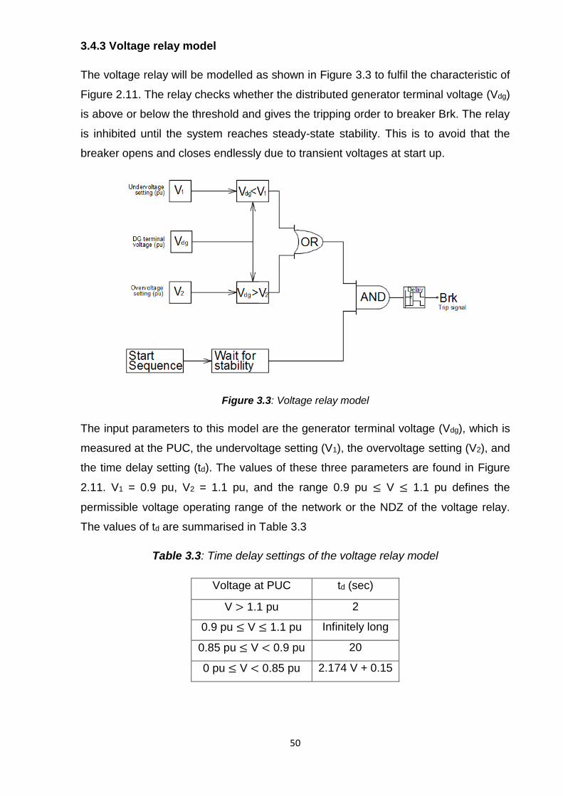
50

3.4.3 Voltage relay model

The voltage relay will be modelled as shown in Figure 3.3 to fulfil the characteristic of

Figure 2.11. The relay checks whether the distributed generator terminal voltage (Vdg)

is above or below the threshold and gives the tripping order to breaker Brk. The relay

is inhibited until the system reaches steady-state stability. This is to avoid that the

breaker opens and closes endlessly due to transient voltages at start up.

Figure 3.3: Voltage relay model

The input parameters to this model are the generator terminal voltage (Vdg), which is

measured at the PUC, the undervoltage setting (V1), the overvoltage setting (V2), and

the time delay setting (td). The values of these three parameters are found in Figure

2.11. V1 = 0.9 pu, V2 = 1.1 pu, and the range 0.9 pu ≤ V ≤ 1.1 pu defines the

permissible voltage operating range of the network or the NDZ of the voltage relay.

The values of td are summarised in Table 3.3

Table 3.3: Time delay settings of the voltage relay model

Voltage at PUC td (sec)

V > 1.1 pu 2

0.9 pu ≤ V ≤ 1.1 pu Infinitely long

0.85 pu ≤ V < 0.9 pu 20

0 pu ≤ V < 0.85 pu 2.174 V + 0.15

51

3.4.4 Lines and transformers models

Lines are represented as lumped RL impedances while transformers are represented

with their equivalent T circuits. The data are presented in Tables 3.4 and 3.5.

Table 3.4: Lines data

Line 1 Line 2

Resistance (mΩ) 36.2 0.362

Inductance (mH) 1.24 0.0124

Table 3.5: Transformers data

Transformer

132/ 33 kV 33/ 0.525 kV

Nominal power (MVA) 50 50

Primary winding Δ Δ

Primary voltage (kV) 132 33

Secondary winding Yn Yn

Secondary voltage (kV) 33 0.525

Resistance (pu) 0 0

Inductance (pu) 0.1 0.1

3.4.5 Excitation system model

The exciter is an IEEE type AC1A exciter, the data of which is given in Table 3.6 (IEEE,

2005: 67).

The simulations that will be carried out in this work require that the generator’s emf is

immune to system disturbances to avoid that such disturbances induce noise that

might unintentionally affect the relay’s anti-islanding performance. It is for this reason

that an IEEE type AC1A exciter was chosen. This exciter does not employ self

excitation and its voltage regulator is powered by an external source that is not affected

by system transients (see section 2.3.8).

52

Table 3.6: Exciter data

TR (s) 0 KF (pu) 0.03 VAMIN (pu) -

14.5 RC (pu) 0 TF (s) 1.0 VRMAX (pu) 6.03

XC (pu) 0 KE (pu) 1.0 VRMIN (pu) -

5.43 KA (pu) 400 TE (s) 0.8 SE[VE1] (pu) 0.10

TA (s) 0.02 KD (pu) 0.38 VE1 (pu) 4.18

TB (s) 0 KC (pu) 0.2 SE[VE2] (pu) 0.03

TC (s) 0 VAMAX (pu) 14.5 VE2 (pu) 3.14

3.4.6 Governor model

The active power output of the generator is considered constant because the

simulation time (1500 ms) is very short. Hence, the speed governor is not modeled.

3.4.7 Synchronous generator model

The generator is a steam turbogenerator. It will be represented with the two-axis model.

The data is presented in Table 3.7.

Table 3.7: Synchronous generator data

Pair of poles 2

Nominal power (MVA) 30

Nominal voltage (V) 525

Inertia constant, H(s) 2.0 Rated angular speed, ωo (rad/s) 314.159

Xd(pu) 1.79

Xd’(pu) 0.169 Xd”(pu) 0.135

Xq(pu) 1.71

Xq’(pu) 0.228

Xq”(pu) 0.2

T’do(s) 4.3 T”do(s) 0.032

T’qo(s) 0.85 T”qo(s) 0.05

Armature resistance (pu) 0.002

Potier reactance, Xp(pu) 0.13

3.4.8 Load model

Islanding is hardest to detect with constant impedance loads (Vieira et al, 2008: 596 -

598) (Vieira et al, 2005: 1661). For this reason loads will be modelled as non-frequency

53

dependent constant impedance loads (IEEE, 1993: 473). Hence, dP/dV = dQ/dV = 2

and dP/df = dQ/df = 0 (see section 2.4.3). The load data is presented in Table 3.8.

Table 3.8: Load data

dP/dV 2

dQ/dV 2 dP/df 0 dQ/df 0

Frequency (Hz) 50

Line rms voltage (kV) 0.525

Rated three-phase real power (MW) 12

Rated three-phase reactive power (MVAR) 9

3.5 Methods of validation of simulation results

The simulation results obtained in this work will be validated against calculation results

or corresponding data of another relay (which we call reference relay) operating in

similar conditions. The intention is to verify that simulation results are reasonable. The

calculated value of an output variable or the corresponding data of a reference relay

will be considered as the expected value of that variable. Then the simulation results

will be compared against it to see how close they come. Two statistical measures of

central tendency will be used to decide how close to the expected result the simulated

results are. These are the standard deviation (σ) and the absolute deviation (Di).

3.5.1 Standard deviation

The standard deviation (σ) of a sample x1...xn of n data points having a mean value or

expected value x is given by equation (3.1):

σ = √1

n−1∑ (xi − x)2n

i=1 (3.1)

A standard deviation close to zero indicates that the data points tend to be very close

to the mean or the expected value of the data set, while a high value of standard

deviation indicates that the data points are spread out over a wider range of values.

In science researchers often report the standard deviation of experimental data. Only

data points that fall farther than 2σ from x are considered a serious deviation.

Deviations within 2 σ of x are seen as caused by normal random error or variation in

the measurements.

54

3.5.2 Absolute deviation

The absolute deviation (Di) of a data point xi of a sample x1...xn of n data points having

a mean value or expected value x is given by equation (3.2):

Di = |xi − x| (3.2)

An absolute deviation close to zero indicates that the data point is very close to the

mean or the expected value of the data set, while a high value of absolute deviation

indicates that the data point is far from the mean value or the expected value of the

data set.

55

4. Setting the frequency relay

4.1 Introduction

Frequency relays employed for the islanding detection of a synchronous generator

must be set so as not to interfere with the normal operation of the network. For that to

be possible, the relay’s anti-islanding performance curve must present an active power

imbalance bigger than the critical active power imbalance. For a given islanding

detection time, the critical active power imbalance will be affected by many operating

parameters including island operating quadrant, load PF and reactive power imbalance

in the island. The objective of this chapter is to investigate how these parameters affect

the anti-islanding performance curve (and hence the critical active power imbalance)

of the frequency relay in order to understand how to safely set the relay when these

parameters are changing. The chapter also investigates the effect of multi-stage

setting on the relay’s ability to detect islanding.

4.2 Simulation procedure

The simulations will use the test system of Figure 4.1.

Figure 4.1: Schematic of the test system

Repeated simulations will be performed to determine relay operating points which will

then be used to plot the performance curve. The procedure to obtain the relay

operating points is described as follows: The active power imbalance in the island is

gradually varied from 0 to 1.0 pu in Q1 and Q4 and from 0 to – 1.0 pu in Q2 and Q3 by

varying the generator active power output. For each active power imbalance value, an

islanding is simulated by opening switch S. Then the pairs of active power imbalance

at bus 4 and relay pickup time are used to project the relay operating points.

56

4.3 Flowchart of the simulation process

Three groups of simulations (impact of the operating quadrant on the relay

performance, impact of load PF on the relay performance, and impact of reactive power

imbalance on the relay performance) are carried out in the following sections, the

ultimate objective of each group of simulations being the determination of conditions

in which islanding is hardest to detect. These conditions form the most pessimistic

cases of islanding detection and inform the setting of the relay. The flowchart of Figure

4.2 pictures the interaction between these groups. Another group of simulations

(impact of multi-stage tripping on the relay performance) is run independently and is

not represented in the flowchart.

Figure 4.2: Flowchart of the simulation process to study the anti-islanding performance of the

frequency relay and set up a guideline for adjusting the relay

57

4.4 Impact of operating quadrant on the relay performance

4.4.1 Simulation results

Figure 4.3 presents the results of the simulations to study the effect of the operating

quadrant on the relay anti-islanding performance. The simulations were carried out on

a load of 12 MVA considering PFs of unity, 0.8 lagging, and 0.9 leading. The reactive

power imbalance in the island was maintained constant at 0.1 pu in Q1 and Q2 and

– 0.1 pu in Q3 and Q4. The relay frequency and time delay settings were fixed at 51

Hz/ 0 ms in Q1 and Q4 and 49 Hz/ 0 ms in Q2 and Q3.

Figure 4.3: Impact of operating quadrant on the performance curve of the frequency relay

4.4.2 Validation of the simulation results

The anti-islanding performance curve of a frequency relay can be plotted using

equation (2.11) which is rewritten here as equation (4.1) for convenience.

t = 2H∆f

fo∆Po(

10.8

)+ td (4.1)

The curve labelled Formula in Figure 4.4 was plotted from this equation. The values

assigned to the different parameters of the equation are: H = 2.0 s, Δf = 1 Hz, td = 0

ms, and fo = 50 Hz.

58

If we consider the calculated value of active power imbalance (ΔP ) for a given islanding

detection time (t) as the expected value, then the sample standard deviation (σ) of a

sample ΔPi…ΔPn consisting of active power imbalances determined by simulation for

the same islanding detection time can be calculated in accordance with equation (3.1)

as follows:

σ = √1

n−1 ∑ (ΔPi − ΔP )2n

i=1 (4.2)

Figure 4.4: Impact of operating quadrant on the performance curve of the frequency relay:

comparison between simulation curves and formula curve

A very close match can be seen between the simulation curves and the formula curve

in Q1 and Q3. In fact, for an islanding detection time of 400 ms, σ equals 0.013 pu in

both quadrants, very close to zero in deed. In contrast σ assimilates a bigger value in

Q2 and Q4 (σ = 0.094 pu in both quadrants). This is because the reactive power

imbalance which is not taken into account in the formula, has a much bigger influence

on the anti-islanding performance of the relay in Q2 and Q4 than it has in Q1 and Q3.

This is elucidated in section 4.4.3.

4.4.3 Analysis and interpretation of the results

As seen in Figure 4.3, for excess of active power cases (Q1 and Q4), the relay is more

sensitive in Q4 than it is in Q1 while for deficit of active power cases (Q2 and Q3) the

relay is more sensitive in Q2 than it is in Q3. Let’s consider the performance curve for

a load PF of 0.8 lagging for example. For an islanding detection time of 400 ms, the

59

critical active power imbalances are 0.175 pu in Q4 versus 0.26 pu in Q1 and – 0.17

pu in Q2 versus – 0.253 pu in Q3. The improved performance of the relay in Q2 and

Q4 can be verified for other PFs and can be explained by what happens right after

islanding.

The deficit of reactive power in Q4 will cause the load voltage and thus the active power

consumed by the load to decay after islanding. Since there is excess of active power

in this quadrant, this will lead to an even bigger excess of active power, which causes

the generator speed, hence the frequency to increase very fast. The result is fast

islanding detection.

The situation is very similar in Q2 where the excess of reactive power forces the load

voltage to increase after islanding and the load to consume more active power. Since

there is already deficit of active power, the increased deficit of active power forces the

generator to decelerate fast. The result is a steep decline in island frequency and a

fast islanding detection.

In Q1 and Q3 the situation is quite different. In these two quadrants, the active and

reactive power imbalances have the same sign (either they are all positive or negative).

As a result, the active power imbalance remains small after islanding and the detection

time is long.

Therefore, when the island operating point is not known or when it is changing, the

setting of the relay must assume operation in Q1 and Q3 since these cases lead to

safe solutions.

4.5 Impact of load power factor on the relay performance

4.5.1 Simulation results

Figure 4.5 presents the results of the simulations to evaluate the effect of load PF on

the relay anti-islanding performance. The simulations were carried out on a load of 12

MVA considering the PFs shown in the figure. The reactive power imbalance in the

island was maintained constant at 0.1 pu in Q1 and – 0.1 pu Q3. The relay frequency

and time delay settings were fixed at 51 Hz/ 0 ms in Q1 and 49 Hz/ 0 ms in Q3.

60

Figure 4.5: Impact of load PF on the performance curve of the frequency relay

4.5.2 Validation of the simulation results

The comparison between the simulation curves and the formula curve is shown in

Figure 4.6. A close match can be observed between these curves indeed. σ equals

0.018 pu in Q1 and 0.016 pu in Q3.

61

Figure 4.6: Impact of load PF on the performance curve of the frequency relay: comparison

between simulation curves and formula curve

4.5.3 Analysis and interpretation of the results

As we can see in Figure 4.5, for a load PF of 0.9 leading and an islanding detection

time of 400 ms in Q1, the critical power imbalance is 0.32 pu. It decreases to 0.3 pu

for unity PF and is even smaller for lagging PFs. Hence, the safest settings are

determined considering the smallest possible leading PF of the local load because it

corresponds to the biggest critical power imbalance. However, if the local load cannot

operate with leading PFs, then unity PF must be assumed.

Similar conclusions can be drawn for operation in Q3, considering absolute values of

power imbalance.

4.6 Impact of reactive power imbalance on the relay performance

4.6.1 Simulation results

Figure 4.7 shows the results of the simulations to study the effect of reactive power

imbalance on the relay anti-islanding performance. The simulations were carried out

on a load of 12 MW, 0 MVAR (PF = 1) considering different values of reactive power

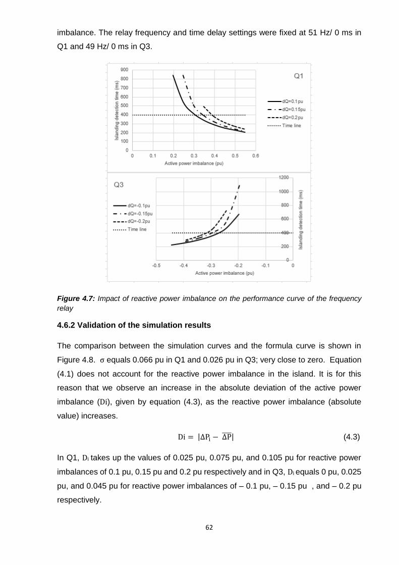
62

imbalance. The relay frequency and time delay settings were fixed at 51 Hz/ 0 ms in

Q1 and 49 Hz/ 0 ms in Q3.

Figure 4.7: Impact of reactive power imbalance on the performance curve of the frequency

relay

4.6.2 Validation of the simulation results

The comparison between the simulation curves and the formula curve is shown in

Figure 4.8. σ equals 0.066 pu in Q1 and 0.026 pu in Q3; very close to zero. Equation

(4.1) does not account for the reactive power imbalance in the island. It is for this

reason that we observe an increase in the absolute deviation of the active power

imbalance (Di), given by equation (4.3), as the reactive power imbalance (absolute

value) increases.

Di = |∆Pi − ∆P | (4.3)

In Q1, Di takes up the values of 0.025 pu, 0.075 pu, and 0.105 pu for reactive power

imbalances of 0.1 pu, 0.15 pu and 0.2 pu respectively and in Q3, Di equals 0 pu, 0.025

pu, and 0.045 pu for reactive power imbalances of – 0.1 pu, – 0.15 pu , and – 0.2 pu

respectively.

63

Figure 4.8: Impact of reactive power imbalance on the performance curve of the frequency

relay: comparison between simulation curves and formula curve

4.6.3 Analysis and interpretation of the results

It is clear from Figure 4.7 that in both Q1 and Q3, islanding is more difficult to detect

with bigger reactive power imbalances (considering absolute values). Let’s consider

for example an islanding detection time of 400 ms in Q1. The active power imbalances

needed to detect islanding are 0.39 pu, 0.35 pu, and 0.3 pu for reactive power

imbalances of 0.2 pu, 0.15 pu, and 0.1 pu respectively. Thus if the operating point is

not known or if it is changing, the setting of the relay must be based on the highest

possible value of the reactive power imbalance in the island.

4.7 Impact of multi-stage tripping on the relay performance

4.7.1 Simulation results

Figure 4.9 shows the results of the simulations to study the effect of multi-stage tripping

on the relay anti-islanding performance. The simulations were performed on a load of

12 MW, 0 MVAR (PF = 1) considering the frequency and time delay settings shown in

64

the figure. The reactive power imbalance was kept constant at 0.1 pu in Q1 and – 0.1

pu in Q3.

Figure 4.9: Impact of multi-stage tripping on the performance curve of the frequency relay

4.7.2 Validation of the simulation results

The comparison between the simulation curves and the formula curves for multi-stage

tripping is shown in Figure 4.10. A close match can be observed between simulation

curves and formula curves for the same frequency and time delay settings. For an

islanding detection time of 1500 ms in Q1, Di takes up the values of 0.03 ms, 0.03 ms,

and 0.06 ms for relay settings of 51 Hz/ 1200 ms, 51.5 Hz/ 800 ms, and 52 Hz/ 400 ms

respectively. The two sets of curves are even more closely matched in Q3 where Di

equals 0.03 ms for 47 Hz/ 200 ms and zero for the other two settings.

65

Figure 4.10: Impact of multi-stage tripping on the performance curve of the frequency relay:

comparison between simulation curves and formula curves

4.7.3 Analysis and interpretation of the results

We observe in Figure 4.9 that for an islanding detection time of 1500 ms, the active

power imbalances necessary to detect islanding in Q1 vary from 0.38 pu for the 51 Hz/

1200 ms curve to about 0.29 pu for the 51.5 Hz/800 ms curve, and 0.285 pu for the 52

Hz/ 500 ms curve. Particularly for the last two curves, we can see that for longer

islanding detection times, multi-stage setting affects the anti-islanding characteristics

of the relay very little. Hence, multi-stage tripping can improve the anti-islanding

performance of the frequency relay by reducing the active power imbalance required

to detect islanding. Similar conclusions may be reached for operation in Q3.

4.8 Guideline for setting the frequency relay

Based on the results of the simulations above, we recommended that the following

guideline be adhered to when adjusting the frequency setting and time delay setting of

a frequency relay to protect a synchronous distributed generator against islanding and

abnormal frequency deviations. Adherence to this guideline will ensure that the relay

is adjusted safely at all times.

66

i) The relay engineer must assume operation in Q1 to determine overfrequency

settings and corresponding time delay settings and operation in Q3 to determine

underfrequency settings and corresponding time delay settings.

ii) The relay engineer must assume unity load PF.

iii) The relay engineer must consider the biggest possible value of reactive power

imbalance (absolute value) that can exist in the island.

iv) The relay engineer must set the relay to trip in multiple stages.

67

5. Setting the voltage relay

5.1 Introduction

Voltage relays employed for the islanding detection of a synchronous generator must

be set so as not to interfere with the normal operation of the network. For that to be

possible, the relay’s anti-islanding performance curve must present a reactive power

imbalance bigger than the critical reactive power imbalance. For a given islanding

detection time, the critical reactive power imbalance will be affected by many operating

parameters including island operating quadrant, load PF, and active power imbalance

in the island. The objective of this chapter is to investigate how these parameters affect

the anti-islanding performance curve (and hence the critical reactive power imbalance)

of the voltage relay in order to understand how to safely set the relay.

5.2 Simulation procedure

The simulations use the test system of Figure 5.1.

Figure 5.1: Schematic of the test system

The reactive power imbalance in the island is varied from 0 to 1.0 pu in Q1 and Q2 and

from 0 to – 1.0 pu in Q3 and Q4 by varying the generator reactive power output. For

each reactive power imbalance value, an islanding is simulated by opening switch S.

Then the pairs of reactive power imbalance value at bus 4 and relay pickup time are

used to plot the performance curve.

5.3 Flowchart of the simulation process

Three groups of simulations (impact of the operating quadrant on the relay

performance, impact of load PF on the relay performance, and impact of active power

imbalance on the relay performance) are carried out in the following sections, the

ultimate objective of each group of simulations being the determination of conditions

68

in which islanding is hardest to detect. These conditions form the most pessimistic

cases of islanding detection and inform the setting of the relay. The flowchart of Figure

5.2 pictures the interaction between these groups.

Figure 5.2: Flowchart of the simulation process to study the anti-islanding performance of the

voltage relay and set up a guideline for adjusting the relay

5.4 Impact of operating quadrant on the relay performance

5.4.1 Simulation results

Figure 5.3 presents the results of the simulations to evaluate the effect of the operating

quadrant on the relay anti-islanding performance. The simulations were carried out on

a load of 12 MVA considering different values of load PF. The active power imbalance

in the island was maintained constant at 0.0333 pu in Q1 and Q4 and – 0.0333 pu in

Q2 and Q3. The relay voltage and time delay settings were fixed at 1.1 pu/ 0 ms in Q1

and Q2 and 0.9 pu/ 0 ms in Q3 and Q4.

69

Figure 5.3: Impact of island operating quadrant on the performance curve of the voltage relay

5.4.2 Validation of the simulation results

The simulation curves are validated against the performance curve of a voltage relay

operating in similar conditions (Vieira et al, 2007: 489). Let’s call the relay against

whose performance curve the validation is done, the reference relay. If we consider

the reactive power imbalance of this relay (ΔQ ) for a given islanding detection time (t)

as the expected value, then the sample standard deviation (σ) of a sample ΔQi…ΔQn

consisting of reactive power imbalances determined by simulation for the same

islanding detection time can be calculated in accordance with equation (3.1) as follows:

σ = √1

n−1 ∑ (ΔQi − ΔQ )2n

i=1 (5.1)

The simulation curves and the reference relay’s curve are compared in Figure 5.4. For

an islanding detection time of 600 ms in Q1 and Q2, a close match can be seen

between these curves. σ equals 0.027 pu in Q1 and 0.022 pu in Q2; fairly close to zero.

Yet, for an islanding detection time of 10 ms, σ increases drastically (σ = 0.209 pu in

Q1 and Q2). This is because the time constant (τ) of the reference circuit (τ = 7.6 ms)

is larger than that of the simulation circuit (τ = 4.5 ms). Accordingly, the reference circuit

voltage takes longer to change after islanding than the simulation circuit voltage.

Similar conclusions apply to Q3 and Q4.

70

Figure 5.4: Impact of operating quadrant on the performance curve of the voltage relay:

comparison between simulation curves and reference curve

5.4.3 Analysis and interpretation of the results

Figure 5.3 demonstrate that the ability of the voltage relay to detect islanding depends

on the combination of active and reactive power imbalances in the island. We can see

that for excess of reactive power cases (Q1 and Q2), the relay is more sensitive in Q1

than it is in Q2 while for deficit of reactive power cases (Q3 and Q4) the relay is more

sensitive in Q3 than it is in Q4. Let’s consider for example the performance curve for a

load PF of 0.9 leading. For an islanding detection time of 600 ms, the reactive power

imbalances are 0.08 pu in Q1 versus 0.1 pu in Q2 and 0.055 pu in Q3 versus 0.0875

pu in Q4. Therefore, when the operating point is not known or when it is changing, the

setting of the relay must assume operation in Q2 and Q4 because these cases lead to

safe solutions.

5.5 Impact of load power factor on the relay performance

5.5.1 Simulation results

Figure 5.5 presents the results of the simulations to evaluate the effect of load PF on

the relay anti-islanding performance. The simulations were carried out on a load of 12

MVA considering the values of load PF shown in the figure. The active power

imbalance in the island was maintained constant at – 0.0333 pu in Q2 and 0.0333 pu

71

in Q4. The relay voltage and time delay settings were fixed at 1.1 pu/ 0 ms in Q2 and

0.9 pu/ 0 ms in Q4.

Figure 5.5: Impact of load PF on the performance curve of the voltage relay

5.5.2 Validation of the simulation results

The comparison between the simulation curves and the reference curve is shown in

Figure 5.6. σ equals 0.022 pu in Q2 for an islanding detection time of 600 ms and 0.209

pu for an islanding detection time of 10 ms. As explained above, the difference in time

constants is the reason for the increased σ near zero ms. In Q4, σ equals 0.013 pu for

600 ms and 0.209 pu for 90 ms.

72

Figure 5.6: Impact of load PF on the performance curve of the voltage relay: comparison

between simulation curves and reference curve

5.5.3 Analysis and interpretation of results

In Q2, Figure 5.5, load PF affects the performance curve on a very narrow range of

reactive power imbalance. Above 0.2 pu, load PF has no effect on the performance

curve as islanding is detected almost immediately no matter the load PF. However,

between 0.05 pu and 0.2 pu, load PF affects the performance curve considerably. For

example, for an islanding detection time of 600 ms, a reactive power imbalance of

about 0.15 pu is required to detect islanding when the load PF is 0.8 lagging. The value

decreases to about 0.12 pu for unity PF and is even smaller for leading PFs. Hence,

the setting of the relay must be based on the smallest possible value of load lagging

PF because this represents the condition in which islanding is hardest to detect.

Similar conclusions can be reached for operation in Q4, considering absolute values

of reactive power imbalance.

73

5.6 Impact of active power imbalance on the relay performance

5.6.1 Simulation results

Figure 5.7 presents the results of the simulations to study the effect of active power

imbalance on the relay anti-islanding performance. The simulations were carried out

on a load of 12 MW, 0 MVAR (PF = 1). The active power imbalance in the island was

varied to study its effect on the performance curve. The relay voltage and time delay

settings were fixed at 1.1 pu/ 0 ms in Q2 and 0.9 pu/ 0 ms in Q4.

Figure 5.7: Impact of active power imbalance on the performance curve of the voltage relay

5.6.2 Validation of the simulation results

The comparison between simulation curves and the reference curve is shown in Figure

5.8.In Q2, σ is close to zero for an islanding detection time of 600 ms and 0.209 pu for

10 ms. As explained above, the difference in time constants is the reason for the

increased σ near zero. In Q4, σ = 0.023 pu for 600 ms and 0.307 pu for 90 ms.

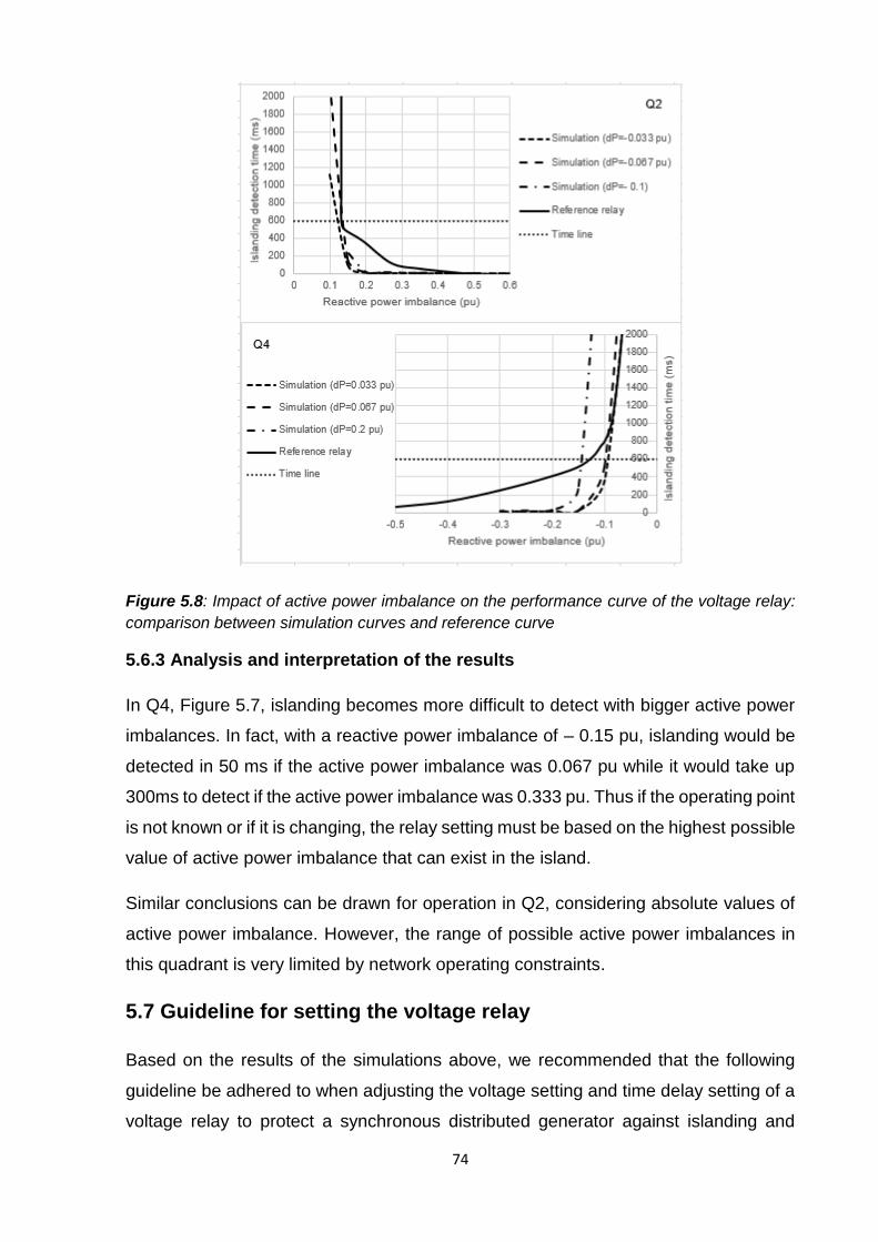
74

Figure 5.8: Impact of active power imbalance on the performance curve of the voltage relay:

comparison between simulation curves and reference curve

5.6.3 Analysis and interpretation of the results

In Q4, Figure 5.7, islanding becomes more difficult to detect with bigger active power

imbalances. In fact, with a reactive power imbalance of – 0.15 pu, islanding would be

detected in 50 ms if the active power imbalance was 0.067 pu while it would take up

300ms to detect if the active power imbalance was 0.333 pu. Thus if the operating point

is not known or if it is changing, the relay setting must be based on the highest possible

value of active power imbalance that can exist in the island.

Similar conclusions can be drawn for operation in Q2, considering absolute values of

active power imbalance. However, the range of possible active power imbalances in

this quadrant is very limited by network operating constraints.

5.7 Guideline for setting the voltage relay

Based on the results of the simulations above, we recommended that the following

guideline be adhered to when adjusting the voltage setting and time delay setting of a

voltage relay to protect a synchronous distributed generator against islanding and

75

abnormal voltage deviations. Adherence to this guideline will ensure that the relay is

adjusted safely at all times.

i) The relay engineer must assume operation in Q2 to determine the overvoltage

settings and corresponding time delay settings and operation in Q4 to determine the

undervoltage settings and corresponding time delay settings.

ii) The relay engineer must consider the smallest possible value of load lagging PF.

iii) The relay engineer must assume the highest possible value of active power

imbalance (absolute value) that can exist in the island.

76

6. Conclusion and future work

6.1 General discussion

Distribution networks are designed for unidirectional power flow from the substation at

high voltage level to consumers at low voltage level. The introduction of a generator

on the distribution line (such a generator is called distributed generator) poses

protection problems. Islanding is one of them.

Islanding occurs when the generator continues to supply loads after the disconnection

of the grid. Islanding poses a problem of safety, power quality, and risk of

asynchronous reclosing. The solution to islanding is to disconnect the generator soon

after it occurs. Many algorithms exist but the frequency relay and the voltage relay

have attracted a lot of interest because of their simplicity and the need to avoid false

tripping, a weak point of anti-islanding relays.

When employed for islanding detection, the frequency relay must satisfy the islanding

detection requirement (maximum time to detect islanding) and the frequency variation

immunity requirement (range of frequency variation for which the generator is required

to remain connected to the network and uphold normal operation). These two

requirements are conflicting because when the relay is set sensitive enough to detect

islanding, it might interfere with the normal operation of the generator, and when it is

set less sensitive to satisfy the frequency variation immunity requirement, it might not

detect islanding timeously.

This conflict is solved by determining the critical active power imbalance of the relay in

the islanding detection time versus active power imbalance graph. In order to satisfy

the islanding detection requirement and the frequency variation immunity requirement

simultaneously, the relay performance curve must present an active power imbalance

bigger than the critical active power imbalance (considering absolute values).

Similarly, to satisfy the islanding detection requirement and the voltage variation

immunity requirement simultaneously, the voltage relay performance curve must

present a reactive power imbalance bigger than the critical reactive power imbalance

(considering absolute values).

77

The aim of this dissertation was to investigate the effect of the following parameters on

the anti-islanding performance characteristics of the frequency relay and the

implication for the relay setting: island operating quadrant, load power factor, and

reactive power imbalance. It was found that islanding was hardest to detect in Q1

(excess of active power and reactive power) and Q3 (deficit of active power and

reactive power) and for the following operating conditions: smallest leading power

factor, and biggest reactive power imbalance (absolute value).

In respect to the voltage relay, the aim was to investigate the effect of the operating

quadrant, load power factor, and active power imbalance on the performance curve

and the implication for the relay setting. It was found that the voltage relay struggles to

detect islanding in Q2 (deficit of active power and excess of reactive power) and Q4

(excess of active power and deficit of reactive power) and for the following operating

conditions: smallest lagging load power factor and biggest active power imbalance

(absolute value).

The dissertation also investigated the effect of multi-stage setting on the anti-islanding

performance of the frequency relay. It was found that multi-stage setting improves the

anti-islanding ability of the frequency relay by reducing the active power imbalance

required to detect islanding.

6.2 Conclusions

To adjust the frequency relay to satisfy both the anti-islanding requirement and the

frequency variation immunity requirement:

i) The relay engineer must assume operation in Q1 to determine overfrequency

settings and corresponding time delay settings and operation in Q3 to determine

underfrequency settings and corresponding time delay settings.

ii) The relay engineer must consider the biggest possible value of reactive power

imbalance (absolute value) that can exist in the island.

iii) The relay engineer must assume unity load PF.

To adjust the voltage relay to satisfy both the anti-islanding requirement and the

voltage variation immunity requirement:

78

i) The relay engineer must assume operation in Q2 to determine overvoltage settings

and corresponding time delay settings and operation in Q4 to determine undervoltage

settings and corresponding time delay settings.

ii) The relay engineer must consider the smallest possible value of load lagging PF.

iii) The relay engineer must assume the highest possible value of active power

imbalance (absolute value) that can exist in the island.

6.3 Future work

There are many modes of control of the synchronous generator but often, it operates

in reactive power control mode or in voltage control mode. Here we have investigated

the impact of island operating quadrant, load PF and reactive power imbalance on the

anti-islanding performance characteristics of the frequency relay with a generator

operating in reactive power control mode. A similar study can be conducted with a

generator operating in voltage control mode.

79

Bibliography

ACKERMANN, T., ANDERSSON, G. and SÖDER, L., 2001. Distributed generation: a

definition. Electric Power Systems Research, 57(3), pp. 195-204.

AFFONSO, C., FREITAS, W., XU, W. and DA SILVA, L., 2005. Performance of

ROCOF relays for embedded generation applications. IEE Proceedings-Generation,

Transmission and Distribution, 152(1), pp. 109-114.

CARLEY, S., 2009. Distributed generation: An empirical analysis of primary motivators.

Energy Policy, 37(5), pp. 1648-1659.

BRIGHT, C., 2001. COROCOF: comparison of rate of change of frequency protection.

A solution to the detection of loss of mains, Developments in Power System Protection,

2001, Seventh International Conference on (IEE) 2001, IET, pp. 70-73.

DRIESEN, J. and BELMANS, R., 2006. Distributed generation: challenges and

possible solutions, Power Engineering Society General Meeting, 2006. IEEE 2006,

IEEE, pp. 8 pp.

FREITAS, W. and XU, W., 2004. False operation of vector surge relays. IEEE

Transactions on Power Delivery, 19(1), pp. 436-438.

FREITAS, W., XU, W., AFFONSO, C.M. and HUANG, Z., 2005. Comparative analysis

between ROCOF and vector surge relays for distributed generation applications. IEEE

Transactions on Power Delivery, 20(2), pp. 1315-1324.

FREITAS, W., XU, W., HUANG, Z. and VIEIRA, J., 2007. Characteristics of vector

surge relays for distributed synchronous generator protection. Electric Power Systems

Research, 77(2), pp. 170-180.

GEIDL, M., 2005. Protection of power systems with distributed generation: state of the

art. ETH, Eidgenössische Technische Hochschule Zürich, EEH Power Systems

Laboratory.

GLOVER, J.D., SARMA, M. and OVERBYE, T., 2011. Power System Analysis &

Design, SI Version. Cengage Learning.

80

GRAINGER, J.J. and STEVENSON, W.D., 1994. Power system analysis. McGraw-Hill

New York.

GRUBB, M. and VIGOTTI, R., 1995. Renewable Energy Strategies for Europe:

Electricity systems and primary electricity sources. Earthscan.

IEEE, 1993. Load representation for dynamic performance analysis. IEEE

Transactions on Power Systems, 8(2), pp. 472 – 482.

IEEE, 2003. Standard for interconnecting distributed resources with electric power

systems: IEEE standard 1547 – 2003. IEEE.

IEEE, 2006. Recommended practice for excitation system models for system stability

studies: IEEE Standard 421.5 – 2005. IEEE.

IPCC, 2011. Press release: Potential of renewable energy outlined in report by the

intergovernmental panel on climate change. Intergovernmental Panel on Climate

Change. Available at: http://srren.ipcc-wg3.de/press/content/potential-of-renewable-

energy-outlined-report-by-the-intergovernmental-panel-on-climate-change

JENKINS, N., ALLAN, R., CROSSLEY, P., KIRSCHEN, D. and STRBAC, G., 2000.

Embedded generation, 1st ed. Bristol, UK: Inst. Elec. Eng.

KUNDUR, P., BALU, N.J. and LAUBY, M.G., 1994. Power system stability and control.

McGraw-Hill, New York.

LOPES, J.P., HATZIARGYRIOU, N., MUTALE, J., DJAPIC, P. and JENKINS, N.,

2007. Integrating distributed generation into electric power systems: A review of

drivers, challenges and opportunities. Electric Power Systems Research, 77(9), pp.

1189-1203.

NERSA, 2012. Grid connection code requirements for renewable power plants

connected to the transmission system or distribution system in South Africa. Draft

version 2.1

O'KANE, P. and FOX, B., 1997. Loss of mains detection for embedded generation by

system impedance monitoring, Developments in Power System Protection, Sixth

International Conference on (Conf. Publ. No. 434) 1997, IET, pp. 95-98.

81

SALMAN, S., KING, D. and WELLER, G., 2001. New loss of mains detection algorithm

for embedded generation using rate of change of voltage and changes in power

factors, Developments in Power System Protection, 2001, Seventh International

Conference on (IEE) 2001, IET, pp. 82-85.

STOFT, S., 2002. Power system economics: Designing markets for electricity. Wiley,

New York.

US DEPARTMENT OF ENERGY, 2010. 2009 Renewable energy data book. US

Department of Energy, New York.

VIEIRA, J., CORREA, D., FREITAS, W. and XU, W., 2005. Performance curves of

voltage relays for islanding detection of distributed generators. IEEE Transactions on

Power Systems, 20(3), pp. 1660-1662.

VIEIRA, J.C.M., FREITAS, W., XU, W. and MORELATO, A., 2006. Performance of

frequency relays for distributed generation protection. IEEE Transactions on Power

Delivery, 21(3), pp. 1120-1127.

VIEIRA, J., FREITAS, W. and SALLES, D., 2007. Characteristics of voltage relays for

embedded synchronous generators protection. Generation, Transmission &

Distribution, IET, 1(3), pp. 484-491.

VIEIRA, J.C.M., FREITAS, W., XU, W. and MORELATO, A., 2008. An investigation on

the nondetection zones of synchronous distributed generation anti-islanding

protection. IEEE Transactions on Power Delivery, 23(2), pp. 593-600.