THERMOELECTRIC OPTIMIZED EFFICIENCY

AT STRONG COUPLING IN NANO-SIZED

PHOTO-ELECTRIC DEVICE

By

SIMACHEW ENDALE ASHEBIR

SUBMITTED IN PARTIAL FULFILLMENT OF THE

REQUIREMENTS FOR THE DEGREE OF

MASTER OF SCIENCE IN PHYSICS

AT

ADDIS ABABA UNIVERSITY

ADDIS ABABA, ETHIOPIA

JUNE 2010

c© Copyright by SIMACHEW ENDALE ASHEBIR, 2010

ADDIS ABABA UNIVERSITY

DEPARTMENT OF

PHYSICS

Supervisor:Dr. MULUGETA BEKELE

Examiners:Dr. MESFIN TSIGE

Dr.TATEK YERGOU

ii

ADDIS ABABA UNIVERSITY

Date: JUNE 2010

Author: SIMACHEW ENDALE ASHEBIR

Title: THERMOELECTRIC OPTIMIZED EFFICIENCY

AT STRONG COUPLING IN NANO-SIZED

PHOTO-ELECTRIC DEVICE

Department: Physics

Degree: M.Sc. Convocation: JUNE Year: 2010

Permission is herewith granted to Addis Ababa University to circulate andto have copied for non-commercial purposes, at its discretion, the above title uponthe request of individuals or institutions.

Signature of Author

THE AUTHOR RESERVES OTHER PUBLICATION RIGHTS, AND NEITHERTHE THESIS NOR EXTENSIVE EXTRACTS FROM IT MAY BE PRINTED OROTHERWISE REPRODUCED WITHOUT THE AUTHOR’S WRITTEN PERMISSION.

THE AUTHOR ATTESTS THAT PERMISSION HAS BEEN OBTAINEDFOR THE USE OF ANY COPYRIGHTED MATERIAL APPEARING IN THISTHESIS (OTHER THAN BRIEF EXCERPTS REQUIRING ONLY PROPERACKNOWLEDGEMENT IN SCHOLARLY WRITING) AND THAT ALL SUCH USEIS CLEARLY ACKNOWLEDGED.

iii

Table of Contents

Table of Contents iv

List of Figures v

Acknowledgements vii

Abstract viii

1 Introduction 1

2 Efficiency at maximum power 7

2.1 Introduction . . . . . . . . . . . . . . . . . . . . . . . . . . . . . . . . . . 7

2.2 Model of the system . . . . . . . . . . . . . . . . . . . . . . . . . . . . . . 7

2.3 Electron dynamics of the model . . . . . . . . . . . . . . . . . . . . . . . . 9

2.4 Thermodynamics of the model . . . . . . . . . . . . . . . . . . . . . . . . 12

3 Optimization of solar energy converter 18

3.1 Optimization Using objective function . . . . . . . . . . . . . . . . . . . . 18

3.2 Optimized efficiency . . . . . . . . . . . . . . . . . . . . . . . . . . . . . . 20

4 Summary and Conclusion 29

Appendix 31

Bibliography 36

iv

List of Figures

1.1 The minimal model of solar energy converter. . . . . . . . . . . . . . . . . 4

2.1 A nano structure photo-electric devices with 2 energy levels, contacts with

two electron reservoir leads at the same temperature but different chemical

potentials from ref.[5]. . . . . . . . . . . . . . . . . . . . . . . . . . . . . . 8

2.2 Schematic view of the nano-sized photo-electric device. The grey arrows

show the different allowed electron transitions. Transitions between the

two energy levels are induced by solar photons (red curved arrows) and by

non-radiative processes (blue curved arrows) from ref.[5]. . . . . . . . . . . 9

2.3 The current of electrons through the device from ref.[5]. . . . . . . . . . . . 11

2.4 The current of electrons through the device with the contribution to the

current due to the interaction with the sun and non-radiative processes

from ref.[5]. . . . . . . . . . . . . . . . . . . . . . . . . . . . . . . . . . . . 12

2.5 Plot of Efficiency at maximum power (green line) compared with Carnot

efficiency (red line)and Curzon Ahlborn efficiency (blue line) versus Carnot

efficiency . . . . . . . . . . . . . . . . . . . . . . . . . . . . . . . . . . . . 15

2.6 Plot of ηC (green line ), ηCA (blue line ) and ηMP (red line) Versus Υ = Ts−TT

15

2.7 Plot of time taken at maximum power for one complete cycle (τmp) versus ηc 17

3.1 Plot of objective function, Ω, versus the free parameter fN for ηc=0.1 . . . 21

3.2 Plot of ηc (red line), ηopt (green line ), ηca (black line ), ηmp (blue line),versus

ηc . . . . . . . . . . . . . . . . . . . . . . . . . . . . . . . . . . . . . . . . . 23

3.3 Plot of ηc (red line ) ,ηopt (blue line ),ηca (green line ) and ηmp (black

line)versus Υ = Ts−TT

. . . . . . . . . . . . . . . . . . . . . . . . . . . . . . 24

3.4 The time taken to complete one full cycle efficiency at maximum power

(blue line) and for optimized efficiency (red line )versus Carnot efficiency . 26

v

3.5 plot of τ rel versus ηc . . . . . . . . . . . . . . . . . . . . . . . . . . . . . . 27

3.6 plot of ηrel versus ηc . . . . . . . . . . . . . . . . . . . . . . . . . . . . . . 27

vi

Acknowledgements

First and foremost, I would like to thank the almighty, God. I would also like to ex-

press my heartfelt appreciation and gratitude to my advisor and instructor Dr. Mulugeta

Bekele for his unreserved support, excellent and generous guidance throughout my work

and making critical reading of my thesis. While working with him, I have got not only

a chance to share his long research experience which benefited me a lot but also how to

build up social life and friendly relationship with people.

I am grateful to all my colleagues of Statistical and Computational Physics group

specially Fistum Borga and Solomon Worku who have delivered their unreserved help

through out my thesis work. I am also thanks to Yeneneh Yalew, Anteneh Getachew and

my finest friend Mequannint Menuy.

Of course, I am very much pleased to foreword my unreserved affection and thank to my

parents. Specially my brother Getasew Endale for his unlimited finical support to have

my own laptop.

Finally, a special thought also goes the department of physics and the school of graduate

studies. I have derived materials from many research journals and books, and I am

indebted to the authors of those publications and books.

vii

Abstract

In this work we consider a model of solar energy converter which is composed of a nano-

scale photo-electric device having two energy levels in contact with two electron reservoir

leads at the same temperature but with different chemical potentials whose task is to

convert radiation energy to electric energy. We analytically study the optimized ther-

modynamic efficiency, which lies between Carnot efficiency and efficiency at maximum

power, of our model displaying strong coupling between the generated electron flux and

the incoming photon flux from the sun. We also find the time taken to accomplish one

complete cycle at the maximum power and at optimized efficiencies.

viii

Chapter 1

Introduction

The area of physics concerned with the relationships between heat and work is thermody-

namics. In its engineering applications thermodynamics has two major objectives. One of

these is to describe the properties of matter when it exists in what is called an equilibrium

state, a condition in which its properties show no tendency to change. The other objective

is to describe processes in which the properties of matter undergo changes and to relate

these changes to the energy transfers in the form of heat and work which accompany

them. Thermodynamics is unique among scientific disciplines in that no other branch of

science deals with subjects which are as commonplace or as familiar. Concepts such as

”heat”, ”work”, ”energy”, and ”properties” are all terms in everyone’s basic vocabulary.

Thermodynamic laws which govern them originate from very ordinary experiences in our

daily lives. In the development of the second law of thermodynamics, it is very conve-

nient to have a hypothetical body with a relatively large thermal energy capacity that can

supply or absorb finite amounts of heat without undergoing any change in temperature.

We call such a body a reservoir. A reservoir that supplies energy in the form of heat is

considered as a source, and one that absorbs energy in the form of heat is considered as

a sink.

Basic thermodynamics tells us about heat engine. A heat engine is any device which,

though a cyclic process, absorbs energy via heat and converts (some of) this energy to

work. Many real world ”engines” (e.g., automobile engine, steam engine) can be modeled

1

2

as heat engines. There are some fundamental thermodynamic features and limitation of

heat engines which arises irrespective of the details of how the engines work. Even if heat

engines differ considerably from one another, all can be characterized by the following

common properties.

1 They receive heat from a high temperature source(e.g., solar energy, oil furnace, nuclear

reactor, etc.).

2 They convert part of this heat to work.

3 They reject the remaining waste heat to a low temperature sink (e.g., the atmosphere,

river, etc.).

4 They operate on a cycle.

A heat engine, while extracting some work, has to transform some amount of heat from a

hot reservoir, at temperature Th, to a cold reservoir, at a low temperature Tc. The ratio

of the useful work, W , extracted to the heat taken from the hot reservoir, Qh, is called

the efficiency, η, of the heat engine; i.e.

η =W

Qh

(1.0.1)

It was Carnot who first showed that no heat engine could convert heat to work better

than the Carnot engine whose efficiency, η, is given by

ηc = 1− Tc

Th

. (1.0.2)

From thermodynamic point of view this efficiency increases as Tc decreases. In other

words, the lower the temperature of the cold system (to which heat is delivered), the

higher the engine efficiency. The maximum possible efficiency, ηc = 1, occurs if the

temperature of cold source is equali to zero and the temperature of the hot source is

3

nonzero. If the reservoir at zero temperature were available as a heat repository, heat

could be freely and completely converted into work and the world ”energy storage” would

not exist [1].

Even though both macroscopic and nano-scale engines work at the same principle, ex-

tensive studies have been done in the performance of mainly macroscopic heat engines[2].

Nowadays, there is much interest in the study of nano-sized heat engines. Some of this

interest lies on the need to have nano-sized engines in order to utilize energy resources

available at these scales, and miniaturization of devices demanding tiny engines operating

on the small scale. As such, modeling nano-sized engines and finding how well they work

(efficiency) is the primary task that has to be considered at present.

To understand how nano-sized photo-electric devices operate as heat engine, we took the

following model that has the minimum ingredients as solar energy converter. The main

part of the solar energy converter is a light absorber (nano structure photo-electric device)

with two energy levels El and Er where the absorption of a photon of light promotes an

electron from the ground state (El) to an excited state (Er).

The solar energy conversion process is now modeled by adding two other states: an elec-

tron reservoir (which accepts an electron from the excited state) and a hole reservoir

(which accepts a ’hole’ from the ground state or, in other words, donates an electron to

the ground state). The free energy per electron in the two reservoirs (in other words, the

chemical potentials) will be denoted by µl and µr but the two lead reservoirs have the

same temperature. In thermal equilibrium µl = µr but in general, µl and µr will not be

equal, and an amount of external work equal to 4µ = µr − µl = qV can be carried out

by transferring an electron from hole reservoir (left lead) to the electron reservoir (right

lead).

4

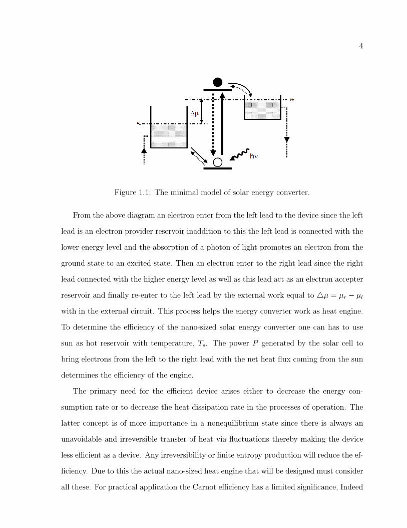
Figure 1.1: The minimal model of solar energy converter.

From the above diagram an electron enter from the left lead to the device since the left

lead is an electron provider reservoir inaddition to this the left lead is connected with the

lower energy level and the absorption of a photon of light promotes an electron from the

ground state to an excited state. Then an electron enter to the right lead since the right

lead connected with the higher energy level as well as this lead act as an electron accepter

reservoir and finally re-enter to the left lead by the external work equal to 4µ = µr − µl

with in the external circuit. This process helps the energy converter work as heat engine.

To determine the efficiency of the nano-sized solar energy converter one can has to use

sun as hot reservoir with temperature, Ts. The power P generated by the solar cell to

bring electrons from the left to the right lead with the net heat flux coming from the sun

determines the efficiency of the engine.

The primary need for the efficient device arises either to decrease the energy con-

sumption rate or to decrease the heat dissipation rate in the processes of operation. The

latter concept is of more importance in a nonequilibrium state since there is always an

unavoidable and irreversible transfer of heat via fluctuations thereby making the device

less efficient as a device. Any irreversibility or finite entropy production will reduce the ef-

ficiency. Due to this the actual nano-sized heat engine that will be designed must consider

all these. For practical application the Carnot efficiency has a limited significance, Indeed

5

a reversible power having no preferred direction in time has to be infinitely slow. Hence

the corresponding power is zero (finite work divided by infinite time). Due to this Curzon

and Ahlborn [3] investigated the problem of efficiency at nonzero power by constructing

a Carnot cycle that operates in a finite time in which the only irreversible steps are as-

sumed to be during the transfers of heat between reservoir and auxiliary work performing

system (the so called endoreversible approximation). Also Van de Broeck [4] proposed

a general derivation within the realm of linear irreversible thermodynamics. This is the

most important feature because it paves the way for analyzing the nonisothermal heat

engines using the linear irreversible thermodynamics frame work, a field upto now almost

limited to isothermal energy converters. Curzon and Ahlborn [3] took an endoreversible

engine that exchange heat linearly at finite rate with the two reservoirs and found its

efficiency, ηCA, at maximum power to be

ηCA = 1−√

Tc

Th

. (1.0.3)

On the other hand, a heat engine operating reversibly is quasistatic and takes infinite

time eventhough its efficiency is maximum. Further more, a heat engine operating at

maximum power takes shortest possible time while dissipating (wasting) high amount of

the input energy and making the device less efficient. A compromise between these two

extremes which leads to decreasing the wastage by relaxing the operating time enough to

optimize energy utilization is of interest in studying such system.

The main purpose of this work is to find the optimized efficiency that lies between Carnot

efficiency and efficiency at maximum power and also the corresponding optimized time

taken to operate one complete cycle.

6

The rest of the thesis is organized as follows. In Chapter two we demonstrate a model

which is considered by B. Cleuren, B. Rutten, M. Esposio of nano sized device having two

single energy levels which is connected with two metal leads of the same temperature that

acts as electrons reservoir where as the sun temperature as the other reservoir. But our

consideration in the case of linear regime that means the sun temperature near to the leads

temperature. We briefly summarize the derivation of efficiency at maximum power and

finally we find the time taken to complete one cycle process. In Chapter three we develop

an objective function based on the proposal of Hernandez et.al.[6] and using optimization

principle we optimize the objective function with respect to the free parameter, fN , after

this we calculate the optimized efficiency of the model and the optimized time taken to

perform one cycle. In the last Chapter we summarize and conclude the results of our

work.

Chapter 2

Efficiency at maximum power

2.1 Introduction

In this chapter we are going to demonstrate the model and the derivation of maximum

power as well as its corresponding efficiency which is presented by B. Cleuren, B. Rutten,

M. Esposio. Finally we calculate the time taken to deliver one cycle process at maximum

power.

2.2 Model of the system

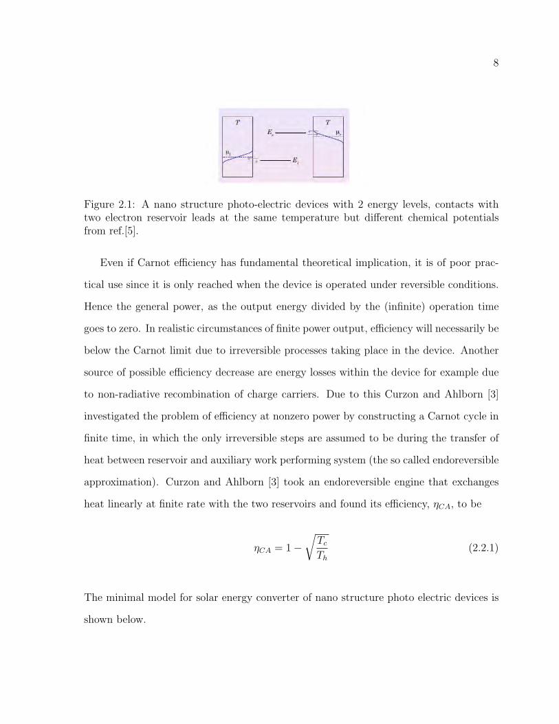
We consider a nano structure photo electric device with two energy levels in contact with

two electron reservoir leads at the same temperature but with different chemical poten-

tials µr = µl + qV whose task is conversion of radiation into electric energy where the

efficiency at which the conversion takes place has universal upper bound given by the

Carnot efficiency ηc = 1− TTs

[1].

A nano structure photo-electric device with two energy levels in contact with two elec-

tron reservoir leads constructed as follows from B. Cleuren, B. Rutten, M. Esposio work.

7

8

Figure 2.1: A nano structure photo-electric devices with 2 energy levels, contacts withtwo electron reservoir leads at the same temperature but different chemical potentialsfrom ref.[5].

Even if Carnot efficiency has fundamental theoretical implication, it is of poor prac-

tical use since it is only reached when the device is operated under reversible conditions.

Hence the general power, as the output energy divided by the (infinite) operation time

goes to zero. In realistic circumstances of finite power output, efficiency will necessarily be

below the Carnot limit due to irreversible processes taking place in the device. Another

source of possible efficiency decrease are energy losses within the device for example due

to non-radiative recombination of charge carriers. Due to this Curzon and Ahlborn [3]

investigated the problem of efficiency at nonzero power by constructing a Carnot cycle in

finite time, in which the only irreversible steps are assumed to be during the transfer of

heat between reservoir and auxiliary work performing system (the so called endoreversible

approximation). Curzon and Ahlborn [3] took an endoreversible engine that exchanges

heat linearly at finite rate with the two reservoirs and found its efficiency, ηCA, to be

ηCA = 1−√

Tc

Th

(2.2.1)

The minimal model for solar energy converter of nano structure photo electric devices is

shown below.

9

Figure 2.2: Schematic view of the nano-sized photo-electric device. The grey arrows showthe different allowed electron transitions. Transitions between the two energy levels areinduced by solar photons (red curved arrows) and by non-radiative processes (blue curvedarrows) from ref.[5].

2.3 Electron dynamics of the model

As shown in the above fig 2.3 the nano device we consider is composed of two single

particle levels of energy El and Er (with Er > El) which define the band gap energy

Eg = Er − El. Assume that coulomb interactions prevent two electrons to be present at

the same time in the device. As a result the device is either empty or has an electron in

level El or Er with respective probabilities pi where i ε0, l, r.

Electron transition between El and Er are induced by two possible mechanisms. The

first is due to incoming sun (black body) radiation at the resonant energy λν = Eg. The

second is due to non-radiative processes at the same resonant transition. The dynamics

of the cell is described using the master equation

∂pi(t)

∂t=

∑j

[kijpj(t)− kjipi(t)], (2.3.1)

which is the gain loss equation for the probability of each state i where the first term of

the above equation is the gain due to the transition of electrons from state j to i and the

10

second term is the loss due to transition of electron into j from i. Using the above relation

we have the master equation to be

p0(t)

pl(t)

pr(t)

=

−kl0 − kr0 k0l k0r

kl0 −k0l − krl klr

kr0 krl −k0r − klr

p0(t)

pl(t)

pr(t)

(2.3.2)

where kij denotes the transition rate from state j to i, pi and pj are probability of state i

and j. The rates describing the exchange of electrons with the leads are given by

kl0 = Γlf(xl); k0l = Γl[1− f(xl)]; kr0 = Γrf(xr); k0r = Γr[1− f(xr)], (2.3.3)

where f(x) = [exp(x)+1]−1 is the Fermi distribution, Γl and Γr are inverse of spontaneous

time taken. The arguments are the scaled energies xl = (El−µl)kBT

and xr = (Er−µr)kBT

while kB

is the Boltzmann constant. The rates describing the transition between energy levels due

to non-radiative (nr) effects and sun photons (s) are given by

krl = Γnrn(xg) + Γsn(xs); klr = Γnr[1 + n(xg)] + Γs[1 + n(xs)], (2.3.4)

where n(x) = [exp(x) − 1]−1 is the Bose-Einstein distribution,Γnr and Γs are inverse of

spontaneous time taken with scaled energies xg = Eg

kBTand xs = Eg

kBTs. Notice that the ra-

tio of the forward and backward transition rates associated to a given elementary process

satisfies the detailed balance condition. This ensures that the equilibrium distribution

(when µl = µr and T = Ts) has the corresponding grand-canonical form.

The following figure shows the electron current entering the device from the left lead is

given by

J = kl0p0 − k0lpl. (2.3.5)

11

Figure 2.3: The current of electrons through the device from ref.[5].

Let us next find the current of the device at steady state defined by p0(t) = pl(t) =

pr(t)=0. J becomes the current of electrons through the device (positive from the left to

the right) with the corresponding electric current qJ . It can be decomposed as J = Js+Jnr

with Js and Jnr being the contribution to the current due to the interaction with the sun

and the non-radiative processes, respectively, and are given by

Js = Γsn(x)pl − Γs[1 + n(x)]pr; Jnr = Γnrn(xg)pl − Γnr[1 + n(xg)]pr, (2.3.6)

12

Figure 2.4: The current of electrons through the device with the contribution to thecurrent due to the interaction with the sun and non-radiative processes from ref.[5].

2.4 Thermodynamics of the model

From a thermodynamic point of view, solar cells are heat engines converting part of the

heat input from the hot reservoir (the sun) into work by moving electrons from lower

to higher chemical potentials. The remaining heat gets transferred to the colder reser-

voir. Since all photons interacting with the solar cell have an energy Eg, the net heat

flux coming from the sun (i.e.the net energy absorbed per unit time) is Qs = EgJs. The

heat flux coming from the cold reservoir has three contributions: Ql = (El − µl)J and

Qr = −(Er − µr)J due to electron exchanges between the cell and the left and the right

lead, respectively, while Qnr = EgJnr is due to the non-radiative energy exchange.

The power P generated by the solar cell to bring electrons from left to the right is given by

P = (µr − µl)J = Ts[xs − (1− ηc)(xr − xl)]J. (2.4.1)

The efficiency at which this conversion takes place is given by

13

η =P

Qs

=(µr − µl)J

(Er − El)Js

= (1− (1− ηc)(xr − xl

xs

))(1 +Jnr

Js

) (2.4.2)

The entropy S(t) of the solar cell can be expressed in the usual form S(t) = −kB

∑i pi(t)lnpi(t).

Its time evolution can be split into a reversible and an irreversible part, S = Se + Si, with

Se = Qs

Ts+ ( Ql

T+ Qr

T+

˙Qnr

T) corresponding to the entropy change due to the heat exchange

with the different reservoirs. Si(≥ 0) can be identified as the internal entropy production

due to dynamical processes with the solar cell [5, 6, 7]. In the stationary regime S = 0 so

that Si = −Se and the entropy production takes on the familiar bilinear form (see more

at the appendix)

Si = QsfU + JfN = (xr − xl)− xsJs − xgJnr (2.4.3)

where fU = 1T− 1

Tsand fN = (µl−µr)

Tare the thermodynamic forces conjugate to the

energy and matter fluxes, respectively.

From now on, we will focus on the linear regime close to thermal equilibrium. In this

regime, characterized by small thermodynamics forces, the heat and the particle flows

appearing in the entropy expression Eq. (2.4.3) can be expanded to first order:

Qs ≈ LUUfU + LUNfN ; J ≈ LNUfU + LNNfN , (2.4.4)

The coefficients Lij appearing are the well known Onsager coefficients. The off-diagonal

elements are responsible for energy conversion process and satisfy the Onsager symmetry

relation LUN = LNU [5, see also the appendix]. For a given temperature difference (quan-

tified by fU), the power from Eq.(3.4.1) becomes P = −TfNJ . So to find the efficiency

at the maximum power, we first maximize the power with respect to the free parameter

14

fN . The engine power takes its maximum value when

∂P

∂fN

∣∣∣∣fmp

N

= 0 (2.4.5)

is satisfied. From Eqs.(2.4.1), (2.4.4) and (2.4.5) the power has maximum value at a finite

value of fmpN which is given by

fmpN = −(

LNU

2LNN

)fU . (2.4.6)

Using Eqs. (2.4.2) and (2.4.6) then the corresponding efficiency, ηmp, at maximum power

becomes

ηmp =ηc

2

κ2

2− κ2. (2.4.7)

This value of ηmp is half the Carnot efficiency multiplied by a factor depending on the

coupling parameter κ = LUN√LUNLNN

[4] which has a numerical value between −1 and +1.

The coupling parameter κ is given by [5]:

κ2 =exl(exg − 1)ΓlΓrΓs

[Γnr(Γl + Γr) + exl((Γnr − Γl)Γr + exgΓl(Γnr + Γr)](Γnr + Γs). (2.4.8)

15

Figure 2.5: Plot of Efficiency at maximum power (green line) compared with Carnotefficiency (red line)and Curzon Ahlborn efficiency (blue line) versus Carnot efficiency

Fig 2.5 shows plot of efficiency versus ηc, that all the efficiencies increases as ηc increase.

Since as ηc increase temperature difference between the two reservoirs increase that means

heat dissipation decrease. Then one can extract more work at highest efficiency than at

lower efficiency. To get finite work at high efficiency ( ηc) one needs to wait for sufficiently

long time but one can extract finite amount of work with in a finite time for efficiency at

maximum power and Curzon and Ahlborn efficiency process.

Let us define dimensionless parameter that describe the model

Υ =Ts

T− 1 (2.4.9)

Figure 2.6: Plot of ηC (green line ), ηCA (blue line ) and ηMP (red line) Versus Υ = Ts−TT

16

Fig 2.6 shows plot of efficiency versus Υ = Ts−TT

, that all the efficiencies increases as

Υ = Ts−TT

increase. Since as Υ = Ts−TT

increase temperature difference between the two

reservoirs increase that means heat dissipation decrease. Then one can extract more work

at highest efficiency than at lower efficiency. To get finite work at high efficiency ( ηc) one

needs to wait for sufficiently long time but one can extract finite amount of work with in

a finite time for efficiency at maximum power and Curzon and Ahlborn efficiency process.

Our next task is to calculate the time taken to complete one cycle when the device

operates at maximum power. From Eqs.(2.4.4) and (2.4.6) with fU = 1T− 1

Ts= ηc

Tthe

corresponding flux at the maximum power becomes

Jmp =LNU

T

ηc

2. (2.4.10)

But it is known that the flux is

J =N

τ. (2.4.11)

where N is number of electrons flowing in time τ across the device. So for one electron

dynamics the flux becomes

J =1

τ. (2.4.12)

Using Eqs.(2.4.9) and (2.4.11) the period, τmp, taken to accomplish one cycle at maximum

power is

τmp =2

ηc

T

LNU

. (2.4.13)

17

Figure 2.7: Plot of time taken at maximum power for one complete cycle (τmp) versus ηc

From Figure 2.7 we observe that the operation time goes to infinity as the Carnot’s

efficiency goes to zero. This happen if the temperature of the reservoirs is the same. So

we can not extract some amount of work with in a finite time for one complete cycle

process to transfer heat from one system to the other. But as Carnot efficiency increase

the time taken for one complete cycle becomes decrease.

Chapter 3

Optimization of solar energyconverter

3.1 Optimization Using objective function

The subject of optimization of real devices has received continued attention in thermo-

dynamics, engineering and recently, in biochemistry [6]. The main goal in optimization

is to find the path way that yields optimum performance in processes operating at non

zero rates. To achieve this goal, an objective function that depends on parameters of the

problem must be optimized. In principle one has the freedom of choice of such function.

It has been pointed out by Hernandez et.al.[6] that a thermodynamic criterion devoted

to analyze the optimum regime of operation in a real process should meet the following

requirements: (i) its dependance on the parameters of the process should be a guidance in

order to improve the performance of that process; (ii) it should not depend on parameters

of environment; and (iii) it should take into account the unavoidable dissipation of energy

provoked by the process. The two most widely used ways in optimization of traditional

thermodynamic heat devices are the entropy generation minimization and exergy analysis

[6]. Exergetic methods additionally depend on the parameters of the environment which

can be unknown or far from the average values [6]. In our work the optimization criteria

as proposed by Hernandez et.al.[6] will be implemented.

18

19

Consider an energy converter that produces a useful energy Eu(y; α), for a given

input energy, Ei(y, α) along a given real process, per cycle provided that it lies between

the maximum, Emax(y, α) and minimum, Emin(y, α), amount of energy that can be

extracted from the energy converter: Emin(y, α) ≤ Eu(y; α) ≤ Emax(y, α). Here

y denotes an independent variable while α denotes a set of parameters which can be

considered as controls. For an energy converter Hernandez et.al.defined two important

quantities: effective useful energy Eu.eff (y; α) as

Eu.eff (y; α) = Eu(y; α)− Emin(y, α), (3.1.1)

and lost useful energy EL.u(y; α) as

EL.u(y; α) = Emax(y; α)− Eu(y, α). (3.1.2)

To evaluate the best compromise between useful energy and lost useful energy we in-

troduce the objective function, defined by Ω, function as the difference between these

quantities

Ω(y, α) = Eu.ef (y; α)− EL.u(y; α). (3.1.3)

Then the conventional efficiency of energy converter defined as the ratio between the use-

ful energy and input energy:

η(y; α) =Eu(y; α)Ei(y, α)

(3.1.4)

20

which satisfies the relation

ηmin(y; α) ≤ η(y; α) ≤ ηmax(y; α) (3.1.5)

where ηmin(y; α) and ηmax(y; α) are the minimum and maximum values of η(y; α)

respectively. Using Eqs.(3.1.1), (3.1.2),and(3.1.4) in Eq.(3.1.3), the expression for Ω is

Ω(y, α) = [2η(y; α)− ηmin(y; α)− ηmax(y; α)]Ei(y, α). (3.1.6)

This equation represents the proposal of Hernandez et.al.[6] as the objective function

to analyze the mode of operation of any energy converter giving the best compromise

between energy benefits and losses. An important feature of the proposed criterion is

that it gives an optimized efficiency that lies between Carnot efficiency and efficiency at

maximum power condition.

3.2 Optimized efficiency

In this section we find that the optimized efficiency that lies between the maximum

efficiency (Carnot efficiency) and the efficiency at maximum power condition by optimizing

the objective function with respect free parameter. From Eq.(3.1.6) we have defined the

objective function

Ω(y, α) = [2η(y; α)− ηmin(y; α)− ηmax(y; α)]Ei(y, α) (3.2.1)

In our case ηmin is the efficiency at maximum power (ηmp) and ηmax is the Carnot efficiency

(ηc) then Eq. (3.2.1) becomes

Ω(y, α) = [2η − ηmp − ηc]Ei(y, α) (3.2.2)

21

where Ei = Wη

. This objective function enable us to analyze the operational mode of our

energy converter giving the best compromise between energy benefits and losses. After

taking the time derivative of Eq.(3.2.2) becomes

Ω = [2η − ηmp − ηc

η]W (3.2.3)

after substituting Eqs. (2.4.2) and (2.4.4) in (3.2.3) our objective function becomes

Ω = −2T [LNUfUfN + LNNf 2N ]− (ηmp + ηc)[LUUfU + LUNfN ] (3.2.4)

The graph of the objective function is given below

Figure 3.1: Plot of objective function, Ω, versus the free parameter fN for ηc=0.1.

Figure 3.1 shows plot of Ω versus fN in which the objective function has an optimum at

a finite value of the free parameter, fN . The efficiency of the device when it operates at

this particular points in the parameter space gives the optimized efficiency, ηopt.

22

After this we optimized the objective function with respect to the free parameter fN .

The objective function takes its optimized value when

∂Ω

∂fN

∣∣∣∣fopt

N

= 0 (3.2.5)

is satisfied. Using Eqs.(2.4.2), (2.4.7), (3.2.4) and (3.2.5) we have

f optN =

−(12− 5κ2)

8(2− κ2)

LNU

LNN

fU (3.2.6)

Finally by using Eqs.(2.4.2), (2.4.4) and (2.2.6) the corresponding optimized efficiency

becomes

ηopt = ηc

[12− 5κ2

8(2− κ2)

][κ2 − ( 12−5κ2

8(2−κ2))κ2

1− ( 12−5κ2

8(2−κ2))κ2

](3.2.7)

where κ is coupling strength. The optimized efficiency at strong coupling (κ = ±1) be-

comes

ηopt =7

8ηc (3.2.8)

23

Figure 3.2: Plot of ηc (red line), ηopt (green line ), ηca (black line ), ηmp (blue line),versusηc

.

Fig. 3.2 shows that all the efficiencies increase as ηc increase. This is because as we

increase ηc the temperature difference of the reservoirs increase. From this we can observe

that the work extracted at Carnot cycle more than work extracted at optimized efficiency

process which is greater than work extracted from Curzon and Ahlborn cycle process.

Where as work extracted from the process of efficiency at maximum power is smaller

than all of the others process. But the time taken to extract work at one complete

cycle of Carnot process is much greater than all other process, and the time taken to

extract work at maximum power the fastest of all the others for one complete cycle.

This because at Carnot cycle process there is no dissipation of energy but there is an

energy dissipation at the process of optimized efficiency and efficiency at maximum power

process. We can therefore say that the operation of the device at optimized efficiency

is indeed a compromise between energy benefits and losses. Since the graph of ηopt lies

between Carnot efficiency and Curzon and Ahlborn efficiency.

24

Figure 3.3: Plot of ηc (red line ) ,ηopt (blue line ),ηca (green line ) and ηmp (black line)versusΥ = Ts−T

T

From fig. 3.3 we see that all the efficiencies increase as Υ = Ts−TT

increase. This is

because as we increase Υ = Ts−TT

the temperature difference of the reservoirs increase.

From this we can observe that the work extracted at Carnot cycle more than work ex-

tracted at optimized efficiency process which is greater than work extracted from Curzon

and Ahlborn cycle process. Where as work extracted from the process of efficiency at

maximum power is smaller than all of the others process. But the time taken to extract

work at one complete cycle of Carnot process is much greater than all other process, and

the time taken to extract work at maximum power the fastest of all the others for one

complete cycle. This because at Carnot cycle process there is no dissipation of energy

but there is an energy dissipation at the process of optimized efficiency and efficiency

at maximum power process. We can therefore say that the operation of the device at

optimized efficiency is indeed a compromise between energy benefits and losses. Since the

graph of ηopt lies between Carnot efficiency and Curzon and Ahlborn efficiency. Finally

we can observe that ηCA and ηmp are overlap for linear regime.

Where as the corresponding value of the flux at the optimized objective function of

25

our system becomes

Jopt = [4− 3κ2

8(2− κ2)]LNUfU (3.2.9)

From Eq.(2.4.11) of section (2.4) the period,τ opt,taken to operate for one cycle at optimized

efficiency becomes

τ opt =8(2− κ2)

4− 3κ2

1

ηc

T

LNU

(3.2.10)

at strong coupling (κ = ±1) the period is

τ opt =8

ηc

T

LNU

(3.2.11)

Relating Eqs.(2.4.12) and (3.2.11) we have τ opt = 4τmp which means the time taken to

complete a process at optimized efficiency four times the fastest process (the process at

maximum power).

The relative time taken under the process of optimized efficiency and efficiency at maxi-

mum power is

τ rel =τ opt − τmp

τmp(3.2.12)

then using Eqs.(2.4.12) and (3.2.11) the relative time taken becomes

τ rel = 3 (3.2.13)

The relative efficiency under the process of optimized efficiency and efficiency at maxi-

mum power is

26

ηrel =ηopt − ηmp

ηmp(3.2.14)

Using Eqs.(2.4.7) and (3.2.8) the relative efficiency becomes

ηrel =3

4(3.2.15)

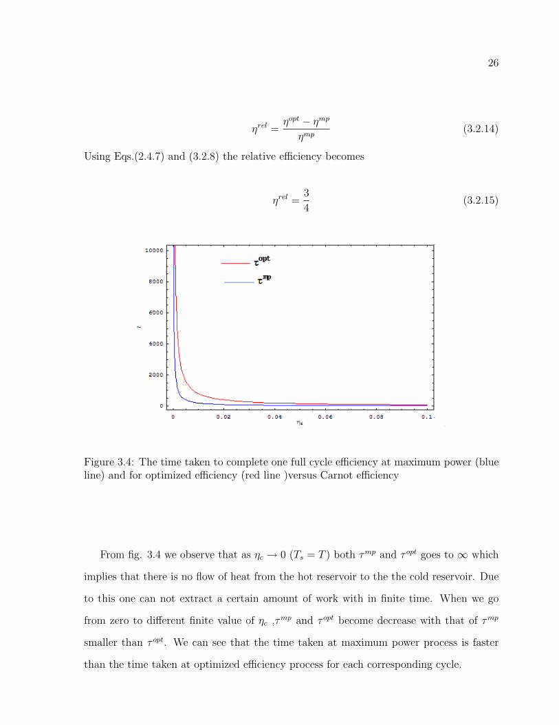
Figure 3.4: The time taken to complete one full cycle efficiency at maximum power (blueline) and for optimized efficiency (red line )versus Carnot efficiency

From fig. 3.4 we observe that as ηc → 0 (Ts = T ) both τmp and τ opt goes to ∞ which

implies that there is no flow of heat from the hot reservoir to the the cold reservoir. Due

to this one can not extract a certain amount of work with in finite time. When we go

from zero to different finite value of ηc ,τmp and τ opt become decrease with that of τmp

smaller than τ opt. We can see that the time taken at maximum power process is faster

than the time taken at optimized efficiency process for each corresponding cycle.

27

Figure 3.5: plot of τ rel versus ηc

From fig. 3.5 we observe that whatever the value of ηc changes, the relative time for

each cycle process is constant that means in what way the temperature of the reservoirs

changed the relative time taken at the process of optimized efficiency and efficiency at

maximum power to extract work in a cycle is constant.

Figure 3.6: plot of ηrel versus ηc

.

28

From fig. 3.6 plot of ηrel versus ηc tell us when we go from small value of ηc (Ts = T ) to

very large value that is Ts > T then ηrel does not change everywhere.

Chapter 4

Summary and Conclusion

In this work, we consider a nano structure photo-electric device with two energy levels

in contact with two electron reservoir leads at the same temperature but with different

chemical potential whose main task is to convert radiation energy to electric energy. We

briefly re-derived the efficiency at maximum power using sun as hot reservoir with tem-

perature Ts, power P generated by the solar cell to bring electrons from the left lead to

the right lead and the net heat flux coming from the sun. In the case of strong coupling

(κ = ±1), where the heat and work producing fluxes are proportional. efficiency at max-

imum power becomes half of the Carnot efficiency. This result is the same as the work

of Curzon and Ahlborn [3]. Furthermore, we calculate the time taken to extract work at

maximum power for one complete cycle.

After we analyzed the efficiency at maximum power for the case of strong coupling and

the corresponding time taken to complete one cycle, we introduce an objective function

based on the proposal of Hernandez et.al.[6]. Using optimization principle we optimized

the objective function with respect to the free parameter, fN , and we found the point at

which the objective function is maximum. We found the optimized efficiency to be exactly

78ηc which is true for strong coupling near the linear regime (Ts ∼ T ). We also calculated

the corresponding optimized time taken to complete one cycle. After this we compared

efficiencies: Carnot efficiency, Curzon and Ahlborn, efficiency at maximum power, and

29

30

optimized efficiency. Carnot efficiency which is the maximum efficiency but it takes in-

finite time to extract certain amount of work. Hence the corresponding power is zero

(finite work divided by infinite time). So for practical application the Carnot efficiency

has a limited significance. Curzon and Ahlborn [3] efficiency at nonzero power in a finite

time but there is dissipation (wastage) of high amount of heat. Efficiency at maximum

power which is the same as Curzon and Ahlborn efficiency at strong coupling as we ob-

serve from the graphs for linear regime. Finally, we have optimized efficiency which lies

between Curzon and Ahlborn efficiency and Carnot efficiency which tells us it is the best

compromise between useful energy and lost energy. But the time taken to complete one

cycle at optimized efficiency four times the fastest time (the time taken to complete one

cycle at maximum power).

In general, we believe that our work has, for the first time, found an efficiency which

is between the efficiency at maximum power (and also Curzon and Ahlborn [3]) and

maximum efficiency (Carnot efficiency) analytically, when the temperature of the sun is

nearly the same as that of lead’s temperature (in linear regime).

We intend to extend our work to the non linear regime to find efficiency at maximum

power, the corresponding time taken to complete one cycle and optimized efficiency as

well as the time taken to accomplish on complete cycle.

Appendix

In this appendix we will derive the expression of entropy production in irreversible ther-

modynamics process and also the Onsager reciprocal relation.

Entropy production in irreversible thermodynamics

process

Irreversible processes can be described in terms of thermodynamic forces and thermody-

namic flows. The thermodynamic flows are a consequence of the thermodynamic forces.

In general, the irreversible change dSi associated with a flow of dX of a quantity such as

heat or matter that has occurred in a time dt. For the flow of heat, we have dX = dQ,

the amount of that followed in a time dt; for the case of matter, we have dX = dN , the

number of moles of the substance that followed in a time dt. In each case the change in

entropy can be written in the form of

dSi = FdX (4.0.1)

in which F is the thermodynamic force. Where the force due to temperature gradient is

given by

F =1

T− 1

T ′ . (4.0.2)

For the flow of matter, the corresponding thermodynamic force is expressed in terms of

31

32

affinity,

F =µ

T− µ

′

T ′ (4.0.3)

All irreversible processes can be described in terms of thermodynamic forces, Fk and the

thermodynamic flows, dXk. We then have the general expression

dSi =∑

k

FkdXk ≥ 0 (4.0.4)

or

dSi

dt=

∑k

FkdXk

dt≥ 0 (4.0.5)

Eq.(4.0.5) embodies the second law of thermodynamics. The entropy production due to

each irreversible process is a product of the corresponding thermodynamic force Fk and

the flow Jk = dXk

dt. If we assume that the entire system is divided into two subsystems,

we not only have

dSi = dS1i + dS2

i ≥ 0 (4.0.6)

in which dS1i and dS2

i are the entropy productions in each sub systems, but we have also

dS1i ≥ 0, dS2

i ≥ 0 (4.0.7)

The total change in entropy, dSi of the system is the sum of the changes of entropy in

each part. The change in entropy due to the flow of heat:

dSi = −dQ

T1

+dQ

T2

= (1

T1

− 1

T2

)dQ. (4.0.8)

Since the heat flows irreversibly from the hotter part to the colder part, dQ is positive if

33

T1 > T2. Hence dSi ≥ 0, in Eq.(4.0.8), dQ and ( 1T2− 1

T1) respectively correspond to dX

and F in Eq.(4.0.1). In terms of the rate flow of heat dQdt

, the rate of entropy production

can be written as

dSi

dt= (

1

T2

− 1

T1

)dQ

dt. (4.0.9)

Now the rate of heat flow or the heat current JQ ≡ dQdt

is given by the laws of heat

conduction. For example according to the Fourier law of heat conduction, JQ = α(T1−T2),

in which α is the coefficient of heat conductivity. Note that the ”the thermodynamic flow

” JQ is driven by the ”thermodynamic force” F = ( 1T1− 1

T2). For the rate of entropy

production we have from Eq.(4.0.9) that

dSi

dt= (

1

T2

− 1

T1

)α(T1 − T2) = α(T1 − T2)

2

T1T2

≥ 0 (4.0.10)

Then the general form of entropy production due to irreversible processes take the quadratic

form

dSi

dt=

∑k

FkdXk

dt=

∑k

FkJk (4.0.11)

in which Fk are the ”thermodynamic forces” where we have represented dXk

dtas the ”flow”

or ”current” Jk. The thermodynamic forces arise when there is non uniformity of tem-

perature, pressure or chemical potential.

34

The Onsager Reciprocal relations

Onsager’s theory begins with the assumption that, where linear phenomenological laws

valid, a deviation αk, decays according to the linear law

Jk =dαk

dt=

∑j

LkjFj. (4.0.12)

From the thermodynamic theory of equilibrium fluctuation the entropy 4Si associated

with fluctuations αi can be written as

4Si = −1

2

∑i,j

gijαjαi =1

2

∑i

Fiαi (4.0.13)

in which

Fk =∂4Si

∂αk

= −∑

j

gkjαj (4.0.14)

is the conjugate thermodynamic force for the thermodynamic flow dαk

dt. Which, by the

virtue of Eq.(4.0.14), can also be written as

Jk =dαk

dt= −

∑j,i

Lkjgjiαi =∑

i

Mkiαi (4.0.15)

in which the matrix Mki is the product of the matrices Lkj and gij. According to the

principle of detailed balance, the effect of αi on the flow (dαk

dt) is the same as the effect of

αk on the flow (dαi

dt). This can be expressed in terms of the correlation function 〈αi

dαk

dt〉

between αi and dαk

dtas

〈αidαk

dt〉 = 〈αk

dαi

dt〉 (4.0.16)

In a way, this correlation isolates that part of the flow dαk

dtthat depends on the variable

αi. Using Eq.(4.0.15) and correlation property we have

〈αidαk

dt〉 =

∑j

Lkj〈αiFj〉. (4.0.17)

35

From Gaussian form of the probability distribution of thermodynamic theory of equilib-

rium fluctuation we have

〈αiFj〉 = −KBδij (4.0.18)

using Eqs.(4.0.17) and (4.0.18) we have

〈αidαk

dt〉 = −KB

∑j

Lkjδij = −KBLki (4.0.19)

similarly

〈αkdαi

dt〉 =

∑j

Lij〈αiFj〉 = −KBLik (4.0.20)

Finally using Eqs.(4.0.19) and (4.0.20)

Lki = Lik (4.0.21)

Eq.(4.0.21) Onsager reciprocal relation

Bibliography

[1] H.B. Callen, Thermodynamics and introduction to thermostatistics 2nd edition

(John Wiley and Sons, 1985).

[2] B. Anderson, P. Salamon, and R. S. Berry, Phys. Today, 37, 62 (1984).

[3] F. L. Curzon and B.Alhborn, Am. J. Phys. 43, 22 (1975).

[4] Van de Broeck, Phys. Rev. Lett. 95, 190602 (2005).

[5] B. Rutten, M. Esposito,, and B. Cleuren, arXiv:0907.4189vl[cond-mat.stat-mech]

23 Jul 2009.

[6] A. Calvo Hernandez, A. Medina, J. M. M. Roco, J. A. White, and S. Velasco, Phys.

Rev. E, 63, 037102 (2001).

[7] Massimiliano Esposito and Katja Lindenberg, Phys. Rev. Lett. 102, 130602

(2009).

[8] J. Schnakenberg, Rev. Mod. Phys. 48, 571 (1976).

[9] A. Beian, J. Appl. Phys. 79, 1191 (1996).

36

37

[10] Dilip Kondepudi, Modern Thermodynamics From Heat Engine to Dissipative

Structures (John Wiley and Sons, 1998).

[11] Ji-Tao Wang, Nonequilibrium Nondisspative Thermodynamics (Springer series in

chemical physics; Vol.68, 2002).

[12] Mesfin Asfaw and Mulugeta Bekele, Eur. Phys. J. 38, 457 (2004).

[13] M. Esposito, K. Lindenberg, and C. Van den Broeck, Phys. Rev. Lett. 102,

130602 (2009).

[14] R. D. Schaller and V. I. Klimov, Phys. Rev. Lett. 92. 186601 (2004).

[15] T. E. Humphrey and H. Linke, Phys. Rev. Lett. 94, 096601 (2005).

[16] A. Calvo Hernandez, J.M.M. Roco, S. Velasco, and A. Medina, Appl.Phys. lett.

73, 853 (1998).

38

Declaration

This thesis is my original work, has not been presented for a degree in any other University

and that all the sources of material used for the thesis have been dully acknowledged.

Name: Simachew Endale

Signature:

Place and time of submission: Addis Ababa University, June 2010

This thesis has been submitted for examination with my approval as University advi-

sor.

Name: Dr. Mulugeta Bekele

Signature: