by tuan tony tran - university of torontotidel.mie.utoronto.ca › pubs › theses ›...
TRANSCRIPT

Decomposition Models for Complex Scheduling Applications
by
Tuan Tony Tran
A thesis submitted in conformity with the requirementsfor the degree of Doctor of Philosophy
Graduate Department of Mechanical and Industrial EngineeringUniversity of Toronto
c© Copyright 2017 by Tuan Tony Tran

Abstract
Decomposition Models for Complex Scheduling Applications
Tuan Tony Tran
Doctor of Philosophy
Graduate Department of Mechanical and Industrial Engineering
University of Toronto
2017
The efficient scheduling of tasks on limited resources is important for many manufacturing and service
industries to keep costs low and efficiently use resources. However, scheduling problems are often difficult
and common scheduling approaches are inadequate for solving problems at the scale necessary for some
applications. Therefore, customized scheduling methods are important for the practical application of
scheduling techniques. The central thesis of this dissertation is that the understanding of the capabilities
of current scheduling technologies and the use of this knowledge to partition a problem into smaller,
more manageable parts that are better suited to these technologies is effective for increasing scheduling
performance. These decompositions advance the state-of-the-art scheduling methodologies and extend
the capabilities of automated scheduling techniques for real-world applications.
In this dissertation, three decompositions have been developed with varying levels of integration
between solvers. Each decomposition addresses the limitations of a technology and improves upon the
current techniques so that they can be used for specific application problems.
The first decomposition model is concerned with scheduling a team of robots in a retirement home.
The scheduler must consider a complex, multi-objective problem, where it must respect user preferences
and schedules. The problem is partitioned into two parts that are each solved using constraint program-
ming. This decomposition shows the improvements that can be obtained when comparing a decomposed
model and a non-decomposed model.
The second application studied is a large-scale data center. Here, jobs arrive dynamically and are
processed on one of approximately 10,000 machines. The decomposition model makes use of techniques
developed in two research areas: queueing theory and scheduling. By segmenting a problem into parts
that are amenable to the techniques from queueing theory and scheduling, a state-of-the-art scheduling
algorithm is crated.
Finally, the third decomposition model combines different paradigms of computation, quantum and
classical computation, into a cohesive algorithm for use in three different scheduling problems. The
hybrid classical computing and quantum computing algorithm develops the capabilities of quantum
annealing, a quantum algorithm run on specialized quantum hardware.
ii
Acknowledgements
I would like to first thank Chris Beck for the past eight years of guidance and supervision. Thank you
for all the patience and support you have given me during our countless hours of meetings. You always
helped me to filter through all my thoughts to develop the good ideas into real contributions. I learned
so much from you and could not have asked for a better mentor. You always held me to a high standard
which resulted in noticeable improvements in everything I do. You are and will continue to be my role
model.
I would also like to thank my co-supervisor Goldie Nejat. You introduced me to the world of robotics
which was a great experience. Thank you for all your insights into the nuances of human-robot interaction
and reminding me of the importance of building scheduling models with positive social impact.
I am grateful to Doug Down, whom I had the privilege of working with for the past eight years.
You were always willing to help work through all my misconceptions in queueing theory and have been
integral to my research since the very start.
I would like to thank my internal committee members Sheila McIlraith and Tim Chan, for their
time, insights, and support. I gained a lot from my meetings and discussions with the two of you to
gain different perspectives on my research. I also thank the members of my final committee, Pascal Van
Hentenryck and Scott Sanner, for their valuable feedback.
I would like to extend my gratitude to Minh Do, Eleanor Rieffel, Jeremy Frank, Zhihui Wang, Bryan
O’Gorman, and Davide Venturelli. I had a great experience at NASA Ames because of the six of you
and I appreciate the opportunity I was given to learn about and play with quantum annealing. I greatly
enjoyed my time working with all of you and continue to enjoy exploring this new and exciting field. In
particular, thank you Minh Do for all that you have done for me. You went out of your way everyday
for all things big and small, welcomed me into your life, and shared so much perspective on your
I would also like to thank Ulas Ozen and Mustafa Dogru for your guidance during my time at Alcatel-
Lucent Bell Labs. I appreciate that the two of you were always willing to give me advice on life in Dublin,
being a graduate student, and what options I have after graduate school.
Thank you to the members of TIDEL, whom I consider to be like family. I have spent the last eight
years getting to know all of you, seeing many leave, and just as many join. Daria Terekhov, you helped
show me that research is something that I would enjoy and I know that, without you, I would have never
gone on to graduate school. Wen-Yang Ku, you have gone through this journey with me, every step of
the way. I am glad that we started together and can end together as we had hoped. I would also like
to especially thank Tiago Stegun Vaquero, Maliheh Aramon Bajestani, Christian Muise, Kyle Booth,
Margarita Castro, Chang Liu, Eldan Cohen, Chiara Piacentini, and Michael Morin for making my time
at TIDEL so much fun. I will miss our long discussions, amazing meals, and crazy antics.
To my parents, grandparents, and sister. Thank you for believing in me and providing me with the
foundation to be who I am today.
Finally, thank you to my wife, An. Without your loving support, I would not have been able to
accomplish any of this. You have been there with me through it all and encouraged me when I was
dispirited, listened to me when I was frustrated, motivated me when I was lost, and inspire me everyday.
iii

Contents
1 Introduction 1
1.1 Dissertation Outline . . . . . . . . . . . . . . . . . . . . . . . . . . . . . . . . . . . . . . . 4
1.2 Summary of Contributions . . . . . . . . . . . . . . . . . . . . . . . . . . . . . . . . . . . . 5
2 Preliminaries 7
2.1 Fundamentals of Scheduling Problems . . . . . . . . . . . . . . . . . . . . . . . . . . . . . 7
2.2 Dispatch Policies . . . . . . . . . . . . . . . . . . . . . . . . . . . . . . . . . . . . . . . . . 10
2.3 Mixed Integer Programming . . . . . . . . . . . . . . . . . . . . . . . . . . . . . . . . . . . 12
2.4 Constraint Programming . . . . . . . . . . . . . . . . . . . . . . . . . . . . . . . . . . . . . 14
2.5 Decomposition Approaches . . . . . . . . . . . . . . . . . . . . . . . . . . . . . . . . . . . 17
2.5.1 Lagrangian Decomposition . . . . . . . . . . . . . . . . . . . . . . . . . . . . . . . 17
2.5.2 Column Generation . . . . . . . . . . . . . . . . . . . . . . . . . . . . . . . . . . . 19
2.5.3 Logic-Based Benders Decomposition . . . . . . . . . . . . . . . . . . . . . . . . . . 21
2.5.4 Ad-Hoc Decompositions . . . . . . . . . . . . . . . . . . . . . . . . . . . . . . . . . 23
2.5.4.1 Incomplete Approaches . . . . . . . . . . . . . . . . . . . . . . . . . . . . 23
2.5.4.2 Complete Approaches . . . . . . . . . . . . . . . . . . . . . . . . . . . . . 24
2.6 Summary . . . . . . . . . . . . . . . . . . . . . . . . . . . . . . . . . . . . . . . . . . . . . 25
3 Planning and Scheduling Mobile Robots in a Retirement Home 26
3.1 Introduction . . . . . . . . . . . . . . . . . . . . . . . . . . . . . . . . . . . . . . . . . . . . 26
3.2 Problem Description . . . . . . . . . . . . . . . . . . . . . . . . . . . . . . . . . . . . . . . 28
3.2.1 Simple Example Problem and Solution . . . . . . . . . . . . . . . . . . . . . . . . . 30
3.2.2 Problem Modifications . . . . . . . . . . . . . . . . . . . . . . . . . . . . . . . . . . 31
3.2.3 Task Representation in Planning and Scheduling . . . . . . . . . . . . . . . . . . . 32
3.2.4 Related Work . . . . . . . . . . . . . . . . . . . . . . . . . . . . . . . . . . . . . . . 33
3.3 PDDL-based Planning . . . . . . . . . . . . . . . . . . . . . . . . . . . . . . . . . . . . . . 34
3.3.1 Domain Modeling . . . . . . . . . . . . . . . . . . . . . . . . . . . . . . . . . . . . 34
3.3.2 Alternative Modeling Strategies . . . . . . . . . . . . . . . . . . . . . . . . . . . . . 40
3.3.3 Problem Modifications . . . . . . . . . . . . . . . . . . . . . . . . . . . . . . . . . . 42
3.3.4 Modeling Issues and Limitations . . . . . . . . . . . . . . . . . . . . . . . . . . . . 43
3.4 Timeline-based Planning and Scheduling . . . . . . . . . . . . . . . . . . . . . . . . . . . . 43
3.4.1 Modeling Issues and Limitations . . . . . . . . . . . . . . . . . . . . . . . . . . . . 45
3.5 Mixed-Integer Programming . . . . . . . . . . . . . . . . . . . . . . . . . . . . . . . . . . . 46
3.5.1 Problem Modifications . . . . . . . . . . . . . . . . . . . . . . . . . . . . . . . . . . 49
iv

3.5.2 Modeling Issues and Limitations . . . . . . . . . . . . . . . . . . . . . . . . . . . . 50
3.6 Constraint-Based Scheduling . . . . . . . . . . . . . . . . . . . . . . . . . . . . . . . . . . 50
3.6.1 Global-CP . . . . . . . . . . . . . . . . . . . . . . . . . . . . . . . . . . . . . . . . . 51
3.6.1.1 Problem Modifications . . . . . . . . . . . . . . . . . . . . . . . . . . . . 57
3.6.1.2 Modeling Issues and Limitations . . . . . . . . . . . . . . . . . . . . . . . 57
3.6.2 Decomposed-CP . . . . . . . . . . . . . . . . . . . . . . . . . . . . . . . . . . . . . 58
3.6.2.1 Modeling Issues and Limitations . . . . . . . . . . . . . . . . . . . . . . . 59
3.7 Experimental Study . . . . . . . . . . . . . . . . . . . . . . . . . . . . . . . . . . . . . . . 60
3.7.1 PDDL-based Planning . . . . . . . . . . . . . . . . . . . . . . . . . . . . . . . . . . 62
3.7.2 Mixed-Integer Linear Programming . . . . . . . . . . . . . . . . . . . . . . . . . . . 64
3.7.3 Constraint Programming . . . . . . . . . . . . . . . . . . . . . . . . . . . . . . . . 65
3.7.3.1 Global-CP . . . . . . . . . . . . . . . . . . . . . . . . . . . . . . . . . . . 66
3.7.3.2 Decomposed-CP . . . . . . . . . . . . . . . . . . . . . . . . . . . . . . . . 66
3.7.4 Best Performance Results . . . . . . . . . . . . . . . . . . . . . . . . . . . . . . . . 66
3.8 Discussion . . . . . . . . . . . . . . . . . . . . . . . . . . . . . . . . . . . . . . . . . . . . . 69
3.8.1 PDDL-Based Planning . . . . . . . . . . . . . . . . . . . . . . . . . . . . . . . . . . 69
3.8.2 Timeline-Based Planning and Scheduling . . . . . . . . . . . . . . . . . . . . . . . 70
3.8.3 Mixed-Integer Programming . . . . . . . . . . . . . . . . . . . . . . . . . . . . . . . 70
3.8.4 Constraint-Based Scheduling . . . . . . . . . . . . . . . . . . . . . . . . . . . . . . 71
3.8.5 The Effect of Modeling . . . . . . . . . . . . . . . . . . . . . . . . . . . . . . . . . 71
3.8.6 AI Planning vs. Constraint Programming . . . . . . . . . . . . . . . . . . . . . . . 72
3.8.7 Decomposition: Benefits and Insights . . . . . . . . . . . . . . . . . . . . . . . . . 73
3.8.8 Future Work . . . . . . . . . . . . . . . . . . . . . . . . . . . . . . . . . . . . . . . 73
3.9 Conclusion . . . . . . . . . . . . . . . . . . . . . . . . . . . . . . . . . . . . . . . . . . . . 74
4 Resource-Aware Scheduling for Heterogeneous Data Centers 76
4.1 Introduction . . . . . . . . . . . . . . . . . . . . . . . . . . . . . . . . . . . . . . . . . . . . 76
4.2 Problem Definition . . . . . . . . . . . . . . . . . . . . . . . . . . . . . . . . . . . . . . . . 78
4.2.1 A Simple Example of the Data Center System . . . . . . . . . . . . . . . . . . . . 79
4.3 Related Work . . . . . . . . . . . . . . . . . . . . . . . . . . . . . . . . . . . . . . . . . . . 80
4.3.1 Algorithms for Comparison: A Greedy Dispatch Policy and the Tetris Scheduler . 82
4.4 LoTES Model . . . . . . . . . . . . . . . . . . . . . . . . . . . . . . . . . . . . . . . . . . . 83
4.4.1 Stage 1: Allocation of Machine Configurations . . . . . . . . . . . . . . . . . . . . 83
4.4.1.1 Example Allocation LP Solution . . . . . . . . . . . . . . . . . . . . . . . 84
4.4.1.2 Rationale for the Fluid Model . . . . . . . . . . . . . . . . . . . . . . . . 85
4.4.2 Stage 2: Machine Assignment . . . . . . . . . . . . . . . . . . . . . . . . . . . . . . 85
4.4.2.1 Example of Bin Generation and Assignment LP . . . . . . . . . . . . . . 89
4.4.2.2 Rationale for the Machine Assignment Problem . . . . . . . . . . . . . . 89
4.4.3 Stage 3: Dispatching Policy . . . . . . . . . . . . . . . . . . . . . . . . . . . . . . . 90
4.4.3.1 Job Arrival . . . . . . . . . . . . . . . . . . . . . . . . . . . . . . . . . . . 90
4.4.3.2 Job Exit . . . . . . . . . . . . . . . . . . . . . . . . . . . . . . . . . . . . 91
4.4.3.3 Example of the Dispatch Policy . . . . . . . . . . . . . . . . . . . . . . . 92
4.4.3.4 Rationale for the Dispatching Policy . . . . . . . . . . . . . . . . . . . . . 92
4.5 Experimental Results . . . . . . . . . . . . . . . . . . . . . . . . . . . . . . . . . . . . . . . 93
v

4.5.1 Implementation Challenges . . . . . . . . . . . . . . . . . . . . . . . . . . . . . . . 93
4.5.2 Google Workload Trace Data . . . . . . . . . . . . . . . . . . . . . . . . . . . . . . 94
4.5.2.1 Machine Configurations . . . . . . . . . . . . . . . . . . . . . . . . . . . . 95
4.5.2.2 Job Class Clustering . . . . . . . . . . . . . . . . . . . . . . . . . . . . . . 95
4.5.2.3 Simulation Results . . . . . . . . . . . . . . . . . . . . . . . . . . . . . . . 96
4.5.3 Randomly Generated Workload Trace Data . . . . . . . . . . . . . . . . . . . . . . 100
4.5.3.1 Machine Configurations . . . . . . . . . . . . . . . . . . . . . . . . . . . . 100
4.5.3.2 Job Class Details: Varying Resource Requirements . . . . . . . . . . . . . 100
4.5.3.3 Job Class Details: Varying Processing Time . . . . . . . . . . . . . . . . 101
4.5.4 Impact of the Offline Stages of LoTES . . . . . . . . . . . . . . . . . . . . . . . . . 103
4.5.4.1 Removing the First Stage of LoTES . . . . . . . . . . . . . . . . . . . . . 103
4.5.4.2 Removing the Second Stage of LoTES . . . . . . . . . . . . . . . . . . . . 103
4.5.4.3 Simulation Results . . . . . . . . . . . . . . . . . . . . . . . . . . . . . . . 104
4.6 Discussion . . . . . . . . . . . . . . . . . . . . . . . . . . . . . . . . . . . . . . . . . . . . . 107
4.6.1 Decomposition: Benefits and Insights . . . . . . . . . . . . . . . . . . . . . . . . . 107
4.6.2 Future Work . . . . . . . . . . . . . . . . . . . . . . . . . . . . . . . . . . . . . . . 108
4.7 Conclusion . . . . . . . . . . . . . . . . . . . . . . . . . . . . . . . . . . . . . . . . . . . . 109
5 A Quantum-Classical Approach to Solving Scheduling Problems 110
5.1 Introduction . . . . . . . . . . . . . . . . . . . . . . . . . . . . . . . . . . . . . . . . . . . . 110
5.2 Quantum Annealing . . . . . . . . . . . . . . . . . . . . . . . . . . . . . . . . . . . . . . . 111
5.2.1 Limitations of Quantum Annealers . . . . . . . . . . . . . . . . . . . . . . . . . . . 113
5.2.2 Related Work . . . . . . . . . . . . . . . . . . . . . . . . . . . . . . . . . . . . . . . 114
5.3 Quantum Annealing Guided Tree Search . . . . . . . . . . . . . . . . . . . . . . . . . . . . 114
5.3.1 Overview of the Framework . . . . . . . . . . . . . . . . . . . . . . . . . . . . . . . 115
5.3.2 Problem Decomposition . . . . . . . . . . . . . . . . . . . . . . . . . . . . . . . . . 118
5.3.3 Solving the Quantum Component . . . . . . . . . . . . . . . . . . . . . . . . . . . 120
5.3.4 Solving the Classical Component . . . . . . . . . . . . . . . . . . . . . . . . . . . . 120
5.3.5 Building the Partial Tree . . . . . . . . . . . . . . . . . . . . . . . . . . . . . . . . 121
5.3.6 Node Pruning . . . . . . . . . . . . . . . . . . . . . . . . . . . . . . . . . . . . . . . 122
5.3.7 Node Selection . . . . . . . . . . . . . . . . . . . . . . . . . . . . . . . . . . . . . . 122
5.3.8 Conditions for Termination . . . . . . . . . . . . . . . . . . . . . . . . . . . . . . . 123
5.4 Problem Domains . . . . . . . . . . . . . . . . . . . . . . . . . . . . . . . . . . . . . . . . . 123
5.4.1 Graph Coloring . . . . . . . . . . . . . . . . . . . . . . . . . . . . . . . . . . . . . . 123
5.4.1.1 Problem Decomposition . . . . . . . . . . . . . . . . . . . . . . . . . . . . 123
5.4.1.2 QUBO Mapping . . . . . . . . . . . . . . . . . . . . . . . . . . . . . . . . 124
5.4.1.3 Node Pruning, Propagation, and the Selection Metric . . . . . . . . . . . 124
5.4.2 Mars Lander Task Scheduling . . . . . . . . . . . . . . . . . . . . . . . . . . . . . . 125
5.4.2.1 Problem Decomposition . . . . . . . . . . . . . . . . . . . . . . . . . . . . 125
5.4.2.2 QUBO Mapping . . . . . . . . . . . . . . . . . . . . . . . . . . . . . . . . 125
5.4.2.3 Classical Component: Battery Considerations . . . . . . . . . . . . . . . 126
5.4.2.4 Node Pruning, Propagation, and the Selection Metric . . . . . . . . . . . 126
5.4.3 Airport Runway Scheduling . . . . . . . . . . . . . . . . . . . . . . . . . . . . . . . 127
5.4.3.1 Problem Decomposition . . . . . . . . . . . . . . . . . . . . . . . . . . . . 127
vi

5.4.3.2 QUBO Mapping . . . . . . . . . . . . . . . . . . . . . . . . . . . . . . . . 128
5.4.3.3 Node Pruning, Propagation, and the Selection Metric . . . . . . . . . . . 128
5.5 Experimental Study . . . . . . . . . . . . . . . . . . . . . . . . . . . . . . . . . . . . . . . 129
5.5.1 Running on the D-Wave 2X Quantum Annealer . . . . . . . . . . . . . . . . . . . . 129
5.5.2 Graph Coloring . . . . . . . . . . . . . . . . . . . . . . . . . . . . . . . . . . . . . . 130
5.5.3 Mars Lander Task Scheduling . . . . . . . . . . . . . . . . . . . . . . . . . . . . . . 131
5.5.4 Airport Runway Scheduling . . . . . . . . . . . . . . . . . . . . . . . . . . . . . . . 132
5.5.5 Comparison to Alternative Solvers . . . . . . . . . . . . . . . . . . . . . . . . . . . 133
5.6 Discussion . . . . . . . . . . . . . . . . . . . . . . . . . . . . . . . . . . . . . . . . . . . . . 135
5.6.1 Decomposition: Benefits and Insights . . . . . . . . . . . . . . . . . . . . . . . . . 135
5.7 Conclusion . . . . . . . . . . . . . . . . . . . . . . . . . . . . . . . . . . . . . . . . . . . . 137
6 Concluding Remarks 139
6.1 Summary . . . . . . . . . . . . . . . . . . . . . . . . . . . . . . . . . . . . . . . . . . . . . 139
6.2 Contributions . . . . . . . . . . . . . . . . . . . . . . . . . . . . . . . . . . . . . . . . . . . 140
6.3 Future Work . . . . . . . . . . . . . . . . . . . . . . . . . . . . . . . . . . . . . . . . . . . 141
6.3.1 Planning and Scheduling Decompositions . . . . . . . . . . . . . . . . . . . . . . . 142
6.3.2 Queueing and Scheduling Decompositions . . . . . . . . . . . . . . . . . . . . . . . 143
6.3.3 Sampling-Based Metaheuristics for Tree Search . . . . . . . . . . . . . . . . . . . . 144
6.3.4 Quantum Annealing for Monte-Carlo Tree Search . . . . . . . . . . . . . . . . . . . 145
A Robot Scheduling: PDDL Details 147
B Robot Scheduling: NDDL Details 157
C Robot Scheduling: Detailed PDDL Results 162
Bibliography 162
vii
List of Tables
3.1 Distance between locations (meters). . . . . . . . . . . . . . . . . . . . . . . . . . . . . . . 30
3.2 Alternative Models . . . . . . . . . . . . . . . . . . . . . . . . . . . . . . . . . . . . . . . . 42
3.3 The number of objects in the five scenarios. . . . . . . . . . . . . . . . . . . . . . . . . . . 60
3.4 Performance of the proposed models on problem BRPOF. The “virtual best” results over
all six PDDL planning models for each scenario is presented. A (-) indicates that no
solution was found. . . . . . . . . . . . . . . . . . . . . . . . . . . . . . . . . . . . . . . . . 61
3.5 Performance of PDDL planning on the BRPOF problem. A (-) indicates that no solution
was found. . . . . . . . . . . . . . . . . . . . . . . . . . . . . . . . . . . . . . . . . . . . . 63
3.6 Performance of PDDL planning on the BRPO- problem. A (-) indicates that no solution
was found. . . . . . . . . . . . . . . . . . . . . . . . . . . . . . . . . . . . . . . . . . . . . 64
3.7 Performance of MIP on all tested problem modifications. A (-) indicates that no solution
was found. . . . . . . . . . . . . . . . . . . . . . . . . . . . . . . . . . . . . . . . . . . . . 65
3.8 Performance of Global-CP on all tested problem modifications. A (-) indicates that no
solution was found. . . . . . . . . . . . . . . . . . . . . . . . . . . . . . . . . . . . . . . . 67
3.9 Performance of the Decomposed-CP model on all tested problem modifications. The
first solution that is recorded is based on the solution found from the first stage of the
Decomposed-CP model. . . . . . . . . . . . . . . . . . . . . . . . . . . . . . . . . . . . . . 68
3.10 Performance of the proposed models using the best modifications. A (-) indicates that no
solution was found. . . . . . . . . . . . . . . . . . . . . . . . . . . . . . . . . . . . . . . . . 69
4.1 Example Machine Configurations. . . . . . . . . . . . . . . . . . . . . . . . . . . . . . . . . 80
4.2 Example Job Classes. . . . . . . . . . . . . . . . . . . . . . . . . . . . . . . . . . . . . . . 80
4.3 Example resource allocation (δjklcjlrkl). . . . . . . . . . . . . . . . . . . . . . . . . . . . . 85
4.4 Example resource allocation (δjkl). . . . . . . . . . . . . . . . . . . . . . . . . . . . . . . . 85
4.5 Example non-dominated bins for Machine Configuration 1. . . . . . . . . . . . . . . . . . 89
4.6 Example non-dominated bins for Machine Configuration 2. . . . . . . . . . . . . . . . . . 89
4.7 Example of jobs being run on machines with available resources for an incoming job. . . . 92
4.8 Machine configuration details for Google workload trace data. . . . . . . . . . . . . . . . . 96
4.9 Job class details. . . . . . . . . . . . . . . . . . . . . . . . . . . . . . . . . . . . . . . . . . 96
5.1 Aircraft types and minimum separation (in seconds). These numbers are based on values
provided by Gupta et al. [113] with modifications to reduce encoding size. . . . . . . . . . 127
viii

5.2 Mean performance for the algorithm variants on the problem instances considered: solving
each instance ten times for each variant. The results from the best α value for the Weighted
variant are used; these values are 0.4, 0.8, and 0.6, for the graph coloring, Mars lander,
and airport runway scheduling problems, respectively. . . . . . . . . . . . . . . . . . . . . 130
5.3 Scheduling information for the Mars lander tasks. . . . . . . . . . . . . . . . . . . . . . . . 131
C.1 Performance of PDDL planning on all tested problem modifications for the single-clock
model. A (-) indicates that no solution was found. . . . . . . . . . . . . . . . . . . . . . . 163
C.2 Performance of PDDL planning on all tested problem modifications for the min-add-clock
model. A (-) indicates that no solution was found. . . . . . . . . . . . . . . . . . . . . . . 164
C.3 Performance of PDDL planning on all tested problem modifications for the set-all-clock
model. A (-) indicates that no solution was found. . . . . . . . . . . . . . . . . . . . . . . 165
C.4 Performance of PDDL planning on all tested problem modifications for the single-envelope
model. A (-) indicates that no solution was found. . . . . . . . . . . . . . . . . . . . . . . 166
C.5 Performance of PDDL planning on all tested problem modifications for the min-add-
envelope model. A (-) indicates that no solution was found. . . . . . . . . . . . . . . . . . 167
C.6 Performance of PDDL planning on all tested problem modifications for the set-all-envelope
model. A (-) indicates that no solution was found. . . . . . . . . . . . . . . . . . . . . . . 168
ix

List of Figures
2.1 A graph coloring problem example represented as a CSP. . . . . . . . . . . . . . . . . . . 15
3.1 Example user schedules. Blue tiles indicate when a user is busy with a personal activity,
red tiles are meal times, green tiles represent the interruptible activities, and white tiles
are leisure periods of time when the users are in their own personal rooms and are available
to interact with robots. . . . . . . . . . . . . . . . . . . . . . . . . . . . . . . . . . . . . . 30
3.2 The UML Class Diagram of the first proposed problem model. Dashed lines represent
an inheritance (e.g., Robot is a type of Mobile) and a solid line represents a relationship
(e.g., a Mobile can be at a Location). . . . . . . . . . . . . . . . . . . . . . . . . . . . . . . 35
3.3 Example of a Bingo game with two participants. The Bingo overall action encompasses all
reminder, setup Bingo, play Bingo, and interact actions associated with the Bingo game.
Here, the setup Bingo action separates the reminders and the Bingo game to ensure that a
minimum amount of time has passed. The length of the Bingo overall action ensures that
the separation of the reminders and the Bingo game is less than the maximum allowed
time. An intuitive representation of the influence of the preconditions and effects of
each action is provided through the use of precedence relationships (arrows) showing the
relative ordering of actions. . . . . . . . . . . . . . . . . . . . . . . . . . . . . . . . . . . . 41
3.4 The UML Class Diagram of the proposed EUROPA model. Dashed lines represent an
inheritance (e.g., Robot is a type of Mobile) and a solid line represents a relationship (e.g.,
a Mobile can be at a Location). . . . . . . . . . . . . . . . . . . . . . . . . . . . . . . . . . 44
3.5 Gantt chart illustrating a sample schedule. Here, telepresence sessions and reminders are
abbreviated as Telepres. and Rem., respectively. . . . . . . . . . . . . . . . . . . . . . . . 52
3.6 Brief overview of the Decomposed-CP model. . . . . . . . . . . . . . . . . . . . . . . . . . 59
3.7 Example user schedules over a single day. Blue tiles indicate when a user is busy with a
personal activity, red tiles are meal times, green tiles represent the interruptible activities,
and white tiles are leisure periods of time when the users are in their own personal rooms
and are available to interact with robots. . . . . . . . . . . . . . . . . . . . . . . . . . . . . 60
4.1 Resource consumption profiles . . . . . . . . . . . . . . . . . . . . . . . . . . . . . . . . . . 78
4.2 Stages of job lifetime. . . . . . . . . . . . . . . . . . . . . . . . . . . . . . . . . . . . . . . 79
4.3 LoTES Algorithm. . . . . . . . . . . . . . . . . . . . . . . . . . . . . . . . . . . . . . . . . 83
4.4 Feasible bin configurations. . . . . . . . . . . . . . . . . . . . . . . . . . . . . . . . . . . . 86
4.5 The number of jobs arriving in each hour in the Google workload trace data. . . . . . . . 95
4.6 Daily proportion of jobs belonging to each job class. . . . . . . . . . . . . . . . . . . . . . 97
x

4.7 Response Time Comparison. . . . . . . . . . . . . . . . . . . . . . . . . . . . . . . . . . . . 98
4.8 Response time distributions. . . . . . . . . . . . . . . . . . . . . . . . . . . . . . . . . . . . 99
4.9 Number of jobs in queue. . . . . . . . . . . . . . . . . . . . . . . . . . . . . . . . . . . . . 99
4.10 Results for varying resource requirements between job classes. . . . . . . . . . . . . . . . . 101
4.11 Results for varying resource requirements between job classes. System load of 0.90. . . . . 102
4.12 Results for varying resource requirements between job classes. System load of 0.95. . . . . 103
4.13 Simulation results for LoTES variations with removed first and second stages. . . . . . . . 105
4.14 Number of bins generated for the data center. . . . . . . . . . . . . . . . . . . . . . . . . . 106
4.15 Number of bins generated for the data center. . . . . . . . . . . . . . . . . . . . . . . . . . 106
4.16 Running time for the offline stages of the scheduler. . . . . . . . . . . . . . . . . . . . . . 107
5.1 Example Chimera graph for a 64-qubit chip. . . . . . . . . . . . . . . . . . . . . . . . . . . 112
5.2 Tree-search based Quantum-Classical Algorithm. . . . . . . . . . . . . . . . . . . . . . . . 115
5.3 Partial binary tree built from three unique solutions: (0, 0, 0), (0, 0, 1), and (1, 1, 0). The
infeasible configurations are represented by the black shaded nodes. Nodes corresponding
to feasible solutions have the subproblem solution (objective value) presented in the node. 117
5.4 Partial binary tree after all open nodes are generated. The infeasible configurations are
represented by the black shaded nodes. Nodes corresponding to feasible solutions have
the subproblem solution (objective value) presented in the node. The open nodes are
indicated by the gray shaded nodes. . . . . . . . . . . . . . . . . . . . . . . . . . . . . . . 117
5.5 Partial binary tree after open nodes are pruned. The infeasible configurations are rep-
resented by the black shaded nodes. Nodes corresponding to feasible solutions have the
subproblem solution (objective value) presented in the node. The open nodes are indicated
by the gray shaded nodes and the pruned nodes are crossed out in red. . . . . . . . . . . . 118
5.6 Fully explored tree. The infeasible configurations are represented by the black shaded
nodes. Nodes corresponding to feasible solutions have the subproblem solution (objective
value) presented in the node. The open nodes are indicated by the gray shaded nodes and
the pruned nodes are crossed out in red. . . . . . . . . . . . . . . . . . . . . . . . . . . . . 119
5.7 Results for the algorithm variants on all graph coloring problem instances: solving each
instance ten times for each variant. The median size of the number of open nodes explored
(left) and the size of the search tree (right) is shown, with error bars at the 35th and 65th
percentiles. Here, search tree size refers to the number of unique leaf nodes (configurations)
found. . . . . . . . . . . . . . . . . . . . . . . . . . . . . . . . . . . . . . . . . . . . . . . . 131
5.8 Solar power production rate for three different scenarios. . . . . . . . . . . . . . . . . . . . 132
5.9 Results for the algorithm variants on the Mars lander task scheduling problem instances:
solving each instance ten times for each variant. The median size of the number of open
nodes explored (left) and the size of the search tree (right) is shown, with error bars at
the 35th and 65th percentiles. Here, search tree size refers to the number of unique leaf
nodes (configurations) found. . . . . . . . . . . . . . . . . . . . . . . . . . . . . . . . . . . 133
5.10 Results for the algorithm variants on the airport runway scheduling problem instances:
solving each instance ten times for each variant. The median size of the number of open
nodes explored (left) and the size of the search tree (right) is shown, with error bars at
the 35th and 65th percentiles. Here, search tree size refers to the number of unique leaf
nodes (configurations) found. . . . . . . . . . . . . . . . . . . . . . . . . . . . . . . . . . . 134
xi

5.11 Results for the alternative algorithms on all problems. The median size of the search tree
is shown, with error bars at the 35th and 65th percentiles. Here, search tree size refers to
the number of unique leaf nodes (configurations) found. . . . . . . . . . . . . . . . . . . . 136
xii

Chapter 1
Introduction
Scheduling, the decision-making process of assigning tasks to resources over time, is found in many
manufacturing and service industries [198]. Regardless of the specific application, resources are typically
limited and the efficient use of these resources is necessary to ensure high performance and low cost.
Within the field of automated scheduling, a number of formalisms and methodologies have been devel-
oped for solving many of these scheduling problems. Although the prevalent scheduling approaches are
successful for solving a considerable number of scheduling problems, even simple models of scheduling
are NP-hard [100]; as such, unless P = NP , there will be specific scheduling problems that present
substantial challenges to existing methodologies and algorithms. Some scheduling problems may have
properties that make them particularly difficult for common scheduling approaches, so customized ap-
proaches that are designed specifically to deal with the complicating properties can be essential to help
improve performance.
This dissertation is concerned with the approach of decomposition, particularly on decompositions
that build upon successful scheduling methodologies such as mixed integer programming (MIP) and
constraint programming (CP). Decomposition partitions a difficult problem into smaller, more manage-
able parts to be solved, and the solutions are united to construct a schedule for the original problem.
A benefit of decomposing a problem is that one can make use of different techniques which are more
amenable to solving each problem partition. If a problem is broken down in an intelligent manner and
the partitions are solved using the appropriate technology, it may be possible to solve difficult scheduling
problems where the non-decomposed approaches are inadequate in practice.
Thesis Statement
The central thesis of this dissertation is that understanding the limitations of a technology,
particularly its modeling and solving capabilities, and partitioning a problem into smaller,
more manageable parts that are amenable to the chosen technology is effective for increas-
ing scheduling performance. These decompositions advance the state-of-the-art scheduling
methodologies and broaden the boundaries of what can be accomplished using available
solvers as a sub-routine within the overall algorithm.
1

Chapter 1. Introduction 2
The Challenges of Decompositions
The challenges of decomposing a problem effectively are the following:
• Choosing which technologies to utilize for a decomposition is non-trivial. To solve any problem, one
must choose a solving technique with strengths and weaknesses compared to alternatives. One must
reason about the modeling capabilities of a formalism and the performance of the available solvers.
However, understanding the behavior of a solver and what aspect of a problem is particularly
challenging for the solver is difficult. Sometimes, it can be apparent, such as a formalism not
having the means to represent a constraint. However, even when representation is not an issue,
a solver can scale very poorly due to some complicating problem aspect. To further confound
matters, a mix of problem aspects can contribute to a solver not being able to solve a problem;
determining these troublesome aspects and how they interact with each other and the solver is not
trivial.
• Deciding how to partition a problem is critical to the success of the model. Creating a decom-
position is a complex task and the appropriate separation of problem aspects depends on the
technologies one has chosen to use (and vice versa). Furthermore, the solutions of all partitions
must be able to be united in such a way that the resulting solution is of high quality and is a fea-
sible solution for the original problem. Therefore, there is a deep connection between the decision
of how to partition a problem and the technique to use to solve the partitions.
Approach of this Dissertation
This dissertation develops decomposition models for complex scheduling problems by understanding the
limitations of a technology and then choosing partitions appropriately. By having a strong grasp of a
solver’s capabilities, it is possible to eliminate complicating aspects of a problem to arrive at a simpler
problem that can be efficiently solved.
The approach taken is that problem simplifications can be the result of a relaxation or restriction.
In problem relaxations, complicating constraints and variables are removed or weakened so that the
resulting problem is easier to solve. However, using a relaxation can lead to an infeasible solution for
the original problem since the constraints and variables are not fully represented. The solution to a
relaxed problem can nonetheless be useful for guiding search techniques towards feasible, high quality
solutions. Restrictions constrain decisions such that the solution space is smaller and the resulting
problem is simpler to solve. In spite of this simplicity, restrictions can remove the optimal solution
from consideration and result in sub-optimal solutions. Regardless, restrictions are useful if one can
intelligently restrict the solution space in a way that solution quality does not suffer significantly, but
computational effort is lowered. The partitions of the original problem are these restricted or relaxed
problems, which alone do not solve the problem of interest. Therefore, one must integrate the various
partitions, which altogether capture the original problem.
The approach focuses more on scheduling applications and building a decomposition for these appli-
cations than on building a general framework. Although the development of a general framework has
many scientific benefits, the interest here is regarding the understanding and improvement of solving
techniques to be used as a sub-routine within a decomposition and how one can apply these decomposi-
tions to scheduling applications. Nonetheless, general frameworks may be developed from this work and

Chapter 1. Introduction 3
some ideas for extensions are presented in the analysis and discussion of the decompositions in Chapters
3 - 5 and in the future directions in Chapter 6.
Proposed Decompositions
Three decompositions are developed, two of which are focused on creating a scheduler for a real-world
application and the last that aims to extend the use of a novel computational model, quantum computing,
to scheduling problems:
1. The first application of interest involves the planning and scheduling of a team of mobile robots
in a retirement home environment. The robots perform various human-robot interaction (HRI)
activities with residents in the home that must take into account the layout of a retirement home,
user schedules and preferences, and physical limitations of the robot (i.e., battery power, velocity,
and charging rates). A two-stage CP-based decomposition is developed that first relaxes the
objective function in the master problem and then reintroduces the full objective function in the
subproblem with restrictions on the decisions based on the master problem solution. An exhaustive
comparison of the decomposed model with non-decomposed models in MIP, artificial intelligence
(AI) planning, and CP is then performed.
2. The second application is the routing and sequencing of tasks in a large-scale data center. Hun-
dreds of jobs arrive each second that must be scheduled onto one of approximately ten thousand
heterogeneous machines. A queueing theory and combinatorial scheduling hybrid decomposition
is proposed that uses a fluid relaxation to guide long-term decision making. The solution to the
queueing model is used to restrict assignment decisions in a combinatorial scheduling model. The
resulting solution to the combinatorial scheduling problem is then integrated into a second, related
queueing model to address long-term decisions while taking into account the complex combina-
torics. In a final step, the solution from the integrated queueing theory and scheduling model is
used to derive an online decision making policy for the dynamic scheduling environment. A com-
parison of the proposed decomposition against two benchmark scheduling policies are performed
using simulation on real workload trace data and randomly generated data.
3. The last decomposition developed is used to investigate quantum computing, specifically quantum
annealing, as a technology for combinatorial scheduling. Due to the current limitations of quantum
annealing, scheduling problems for the most part cannot be solved using quantum computers.
The goal is to build a decomposition model that can enable the use of quantum annealing for
scheduling problems. A hybrid classical computing and quantum computing tree search framework
is introduced that uses a quantum annealer to generate solutions to a relaxed problem. These
solutions are used to construct a search tree that is managed by a classical computer, which stores
the tree, prunes nodes, and solves restricted problems to ensure the solutions from the quantum
annealer are either feasible solutions or can be extended to a feasible solution.
Each approach addresses different levels of decompositions, from using a single technology to hy-
bridizing increasingly diverse technologies. The first decomposition considers only CP and compensates
for the weaknesses of the solver by stripping away the complexities of a problem until a simpler problem
can be efficiently solved. Two problem partitions are solved using CP, resulting in a decomposition that
is fast and can consistently produce high quality solutions. The second decomposition uses ideas from

Chapter 1. Introduction 4
two different research areas: queueing theory and scheduling. These two research areas complement
one another as queueing theory has focused on stochastic system dynamics and scheduling is concerned
with combinatorial optimization. A system that has both properties can benefit from the hybridization
of these two areas so that both dynamic and combinatorial properties are appropriately represented
and reasoned about. Finally, a decomposition is considered that integrates two different paradigms of
computation: quantum computing and classical computing. The limitations of an existing specialized
quantum computing algorithm, quantum annealing, is addressed and the algorithm is augmented with
a classical computing component.
1.1 Dissertation Outline
Chapter 2 provides a review of the literature on automated scheduling and methodologies commonly
used to solve scheduling problems. Scheduling dispatch policies and the use of CP and MIP in the
context of scheduling are presented. The chapter concludes with a review of decomposition methods,
classified based on whether the partitions are a relaxation or restriction of the original problem.
The planning and scheduling of a team of mobile robots in a retirement home is studied in Chapter 3.
The problem lies at the intersection of planning and scheduling, where the system manager must reason
about whether a task is to be executed or not, temporal constraints regarding these tasks and the
residents of the retirement home, and the resource usage of rooms, power, and robots. Comparisons
are made between four different methodologies: planning, timeline-based planning, MIP, and CP. From
the study of these methodologies and the solvers of these formalisms, insights are obtained into the
complicating aspects of the problem which are found to be difficult for the solvers to handle. Based on
these insights, a CP-based decomposition is developed that outperforms all alternative models.
Chapter 4 addresses the dynamic, online scheduling of a data center environment. This work considers
a system with dynamism and uncertainty, properties that do not exist in the majority of scheduling
research [16, 198]. Typically, scheduling systems are static, where all jobs and the parameters relevant for
scheduling these jobs are known a priori. Although works regarding dynamic and stochastic scheduling do
exist, these models are generally too slow to be of use in practice for a data center or consist of myopic
dispatch policies that ignore the system dynamics. A queueing theory and combinatorial scheduling
hybrid model is developed that makes use of the former to provide long-term guidance based on system
level behavior and the latter to handle the combinatorics required to ensure efficient usage of resources.
The partitioning scheme allows us to make full use of the strengths of queueing theory and scheduling,
while compensating for their weaknesses. An empirical investigation using real Google workload trace
data and generated data show the benefits of the proposed decomposition over two benchmark scheduling
algorithms.
Continuing the study of integrating two different research areas, Chapter 5 extends the integration
to two different models of computation: classical computing and quantum computing. The use of
quantum annealing, a metaheuristic algorithm using specialized quantum hardware, has been heavily
limited due to it being a nascent technology. The examination of the limitations of quantum annealing
guided the development of a hybrid quantum-classical algorithm that is able to compensate for some
of these hindrances. A study of the search algorithm and an empirical evaluation of the framework on
three scheduling problems provides a proof-of-concept for the application of quantum annealing within
a quantum-classical hybrid algorithm.

Chapter 1. Introduction 5
Chapter 6 presents a summary of this dissertation and its contributions followed by a discussion on
potential research directions that build on work done in this dissertation.
Appendix A and B include the planning domain definition language (PDDL) model and new domain
definition language (NDDL) model details for Chapter 3, respectively. Appendix C presents extended
results for the different solvers tested in Chapter 3.
1.2 Summary of Contributions
The interests and approaches of this dissertation are from an engineering perspective, focused on de-
veloping decomposition-based techniques to solve challenging scheduling problems. The contributions
add insight and understanding to the performance of decomposition models designed for a scheduling
application, providing data points that can be subsequently used to extend the proposed models to more
general frameworks. Generalizations in the analysis and discussion of the decompositions are pointed
out, however the main contribution is on the development of decomposition-based approaches to solve
hard problems. The main contributions of this work are listed below.
Planning and Scheduling a Team of Mobile Robots in a Retirement Home
(Chapter 3)
1. A complex multi-robot HRI problem is modeled with four different solving technologies: AI Plan-
ning, Timeline-Based Planning and Scheduling, MIP, and CP. Direct comparisons between these
technologies are uncommon as each formalism contains its own assumptions, restrictions, and
solving techniques that affect how one can and should develop a model.
2. A CP-based decomposition model is developed that outperforms all other tested approaches. Re-
sults from a CP model provide insights on the short-comings of the technology to handle some
aspects of the robot task scheduling system; these insights are then used to create an appropriate
decomposition. The decomposition ignores one complicating aspect of the problem in the first
stage, and then reduces the search space of the problem in the second stage by using the result-
ing solution of the first stage. Following this decomposition allows us to consistently obtain high
quality solutions.
3. Alternative models in Planning Domain Definition Language (PDDL) are investigated for timed
events and multi-user actions. The principles and practice of taking a real problem and developing
a model are not often discussed and alternative models tend to not be explored in depth in the
planning community. This work contributes to the study of effective modeling.
4. This work introduces one of the first applications of CP to a multi-robot planning and schedul-
ing problem. Automated planning is commonly proposed for handling decision making in robot
systems. The results show that CP is a strong candidate with great potential to providing high
quality schedules.
Resource-Aware Scheduling for Heterogeneous Data Centers (Chapter 4)
1. A hybrid queueing theoretic and combinatorial optimization scheduling algorithm is proposed for a
data center. By decomposing the problem, it is possible to address both the system dynamics and

Chapter 1. Introduction 6
complex combinatorics, providing a richer representation of the system than would be commonly
found in pure queueing theory or combinatorial scheduling approaches.
2. The allocation linear programming (LP) model [8] used for distributed computing [6] is extended
to a data center that has machines with multi-capacity resources. A system with multi-capacity
resources can have idle resources because it cannot execute a set of jobs that simultaneously use
all the resources of a machine. Thus, the model is more complex than the original allocation LP
model as it is important to account for these idle resources to accurately represent the behaviour
of the system.
3. An empirical study of the scheduling algorithm is performed on both real workload trace data and
randomly generated data that shows that the decomposition performs orders of magnitude better
than existing techniques.
A Quantum-Classical Approach to Solving Scheduling Problems (Chapter 5)
1. A novel framework for quantum-classical hybrid approaches to combinatorial problems is proposed.
This framework is one of the first quantum-classical hybrid algorithms developed.
2. The first implementation of a quantum-classical decomposition that is actually run on quantum
hardware is performed. Until now, no other works have integrated a quantum computer and a
classical computer within a single hybrid framework.
3. The first use of quantum annealing in a complete search is introduced. Quantum annealing is a
stochastic solver and is not itself a complete technique. Through the use of the proposed decom-
position, the quantum annealer is used as a sub-routine within a complete search framework.

Chapter 2
Preliminaries
This chapter describes the necessary background and notation required for the majority of the disserta-
tion. A description of fundamental concepts and notation for scheduling problems is first provided as an
overview of the type of problem that is of interest. A presentation of different scheduling methodologies
then follows, comprising of common solution approaches to scheduling problems that are used in the
decompositions developed in this dissertation. The final section in this chapter discusses decomposition
approaches in the literature to provide context for the proposed decompositions.
2.1 Fundamentals of Scheduling Problems
The study of scheduling is concerned with the allocation of scarce resources to tasks over time [199].
Resources and tasks can represent different real-world objects based on the application of interest. In
this dissertation, Chapter 3 considers robots as resources and activities executed by robots as tasks.
Chapter 4 represents computing machines in a data center as resources and incoming jobs as tasks.
Finally, Chapter 5 studies different problems, where a Mars lander or an airport runway are resources
and Mars lander jobs or flights are tasks.
A task, j, in a scheduling problem is usually defined by four static pieces of data [198]:
• A processing time on a resource i, pij , that is the amount of time for which task j requires the use
of machine i. If the processing time does not depend on the machine, index i can be dropped and
the processing time is denoted as pj .
• A release date, rj , representing the earliest time at which the task can start its processing.
• A due date, dj , which is the date by which a task should be completed.
• A weight, wj , that is the priority factor of a task reflecting its importance.
These four pieces of data are considered static data, since they do not depend on the schedule.
Alternatively, Pinedo [198] defines dynamic data as data that are not fixed in advance and depend
on the schedule. The important dynamic data are:
• The start time of task j on machine i, sij .
• The completion time of task j on machine i, cij .
7

Chapter 2. Preliminaries 8
A valid schedule is one which assigns a start and completion time on a machine for each task, sij and
cij , while adhering to all problem constraints. In general, the start and completion time of a task can
be denoted without the dependence on a machine i as just sj and cj .
A scheduling problem is comprised of three components [108]: the machine environment, the pro-
cessing characteristics and constraints, and the objective function.
The machine environment states the number of machines and the relations among them. Pinedo
[198] discusses four such systems:
• A single machine model that processes all tasks, denoted as 1.
• Parallel machines denoted as Rm, where there are m machines that tasks are processed on. Tasks
must be assigned to one of the m machines and not all machines need to be identical; studies have
looked at both identical [42, 156] and non-identical parallel machines [157, 235].
• A flow shop denoted as Fm, where there are m ordered machines and every task must to be
processed on each machine following the machine order.
• A job shop denoted as Jm, where there are m machines that tasks are processed on, but unlike a
flow shop, each task may have a different route for processing on machines.
The second component describing a scheduling problem is the processing characteristics and con-
straints. Here, five constraints that are used in this dissertation are explained:
• Time windows (rj , dj): Each task has associated with it a release date, rj , and due date, dj ,
which describes a time window. Each task should start and end within its time window, but some
scheduling problems may allow tasks to complete after their due date with an associated penalty.
If there is a date by which the task must absolutely be completed, it is referred to as a deadline.
Time windows are used in Chapters 3 and 5.
• Precedence (prec): Precedence constraints describe an ordering between two tasks and imply that
the processing of one task must be finished before the start of another. Precedence constraints are
used in Chapters 3 and 5.
• Machine capacity (C): Machines can be unary or multi-capacity. Unary capacity machines are
restricted to only processing a single task at a time (C = 1). Multi-capacity machines have some
capacity C > 1 where the capacity required by all tasks that are concurrently executed on the
machine must sum to less than or equal to C. Unary capacity machines are used in Chapters 3
and 5 and multi-capacity machines in Chapter 4.
• Resource constraint (W ): Tasks may require a specific operator or tool and might consume some
limited resource, W . Typically an operator or a tool will be used during processing of a task
and released upon completion. The consumption of resources can also be permanent which will
eventually deplete a reservoir of the resource, although in some instances, it may be possible to
replenish the reservoir during execution of the schedule. An example of a resource reservoir is the
battery capacity of a robot; performing actions consumes energy, but the battery can be recharged
from a power source. Resource capacity is used in Chapters 3 to 5.

Chapter 2. Preliminaries 9
• Setup times (sjk): Between processing of successive tasks j and k, a setup time may be required,
sjk, which can commonly represent tool changes on a machine or travel time between locations of
the two tasks. A machine is busy during the setup time and this time may depend on the ordering
of the two tasks. For example, sequence-dependent setup times may occur in paint mixing facilities,
where different paint colors require different levels of cleaning when followed by another paint color
[182]. Setup times are used in Chapters 3 and 5.
The last component to describe a scheduling problem is the objective. Most common scheduling
objectives can be divided into two categories: time-based objectives and cost-based objectives. The
former are typically concerned with the completion time of tasks, cj . Popular objectives related to the
completion time of tasks include [198]:
• Makespan (Cmax): The latest completion time over all tasks, denoted Cmax. Here, the objective
is to complete all tasks as quickly as possible.
• Weighted completion time (∑wjcj): Here, it is important to consider the completion time of all
tasks rather than just the latest task as is done with makespan minimization.
• Weighted lateness (∑wjLj): The lateness of a task is calculated as Lj = cj − dj . Tasks can be
completed after their due date, but a cost is incurred. If a task is completed earlier than its due
date, a reward is received.
• Maximum lateness (Lmax): The task that is the latest is considered, denoted as Lmax. Here, it is
important to ensure that the lateness of the task with the worst performance is minimized rather
than to reduce the lateness of all jobs.
• Weighted tardiness (∑wjTj): The tardiness of a task is calculated as Tj = max(0, cj − dj). Here,
the objective only penalizes late tasks and does not reward early completions.
• Weighted number of tardy tasks (∑wjUj): Uj is a binary variable that equals 0 if cj ≤ dj and
1, otherwise. This objective penalizes a task that is completed after its due date, but does not
increase the penalty in relation to how late a task is completed.
The cost-based objectives commonly are [198]:
• Setup costs (∑yjkσjk): In some problems, a significant cost can be attributed to setups. However,
these costs may not be proportional to their duration and so the cost of the setup must be con-
sidered. For example, a setup time on a machine with ample capacity may not affect the overall
performance of a schedule in terms of the time-based objectives, but may produce a large amount
of material waste. Given yjk a binary decision variable that equals 1 if and only if task j directly
precedes task k and σjk as the cost of a setup between tasks j and k, the total setup cost of a
schedule is∑yjkσjk.
• Inventory costs (∑itht): An important objective in many manufacturing facilities is the mini-
mization of Work-In-Progress (WIP) inventory or finished goods inventory that represents invested
capital and space. Keeping inventory for extended periods of time can be costly and working to-
wards having less or no inventory is a popular objective that has led many companies in Japan,
such as Toyota, to adopt the Just-In-Time (JIT) concept [178]. If it represents the amount of WIP
at time period t and ht is the holding cost, then∑itht expresses the inventory cost.

Chapter 2. Preliminaries 10
• Transportation costs (∑yjktjk): Transportation costs can be likened to setup costs, except these
costs are directly due to costs incurred by moving materials between locations. These costs may
or may not be independent of the distance travelled and are denoted as tjk, the cost of travelling
between locations of task j and k.
Although a number of objectives are presented here, there are many other objectives that can be used
as each scheduling application may define utility in different ways. For example, Chapter 3 in this
dissertation looks at a cost-based objective of maximizing the number of occurrences of a particular
activity (Bingo game participation) and is an objective that is unique to the problem domain as most
of the literature on scheduling has been focused more heavily towards manufacturing facilities [198].
Finally, it is important to distinguish between offline and online scheduling problems. In offline
scheduling problems, the scheduler is provided with complete information regarding tasks and machines
prior to any scheduling decisions. The scheduler must then generate a complete schedule prior to the
start of execution. Chapters 3 and 5 are concerned with offline scheduling problems. In contrast,
the scheduler in online problems does not have complete information in advance. Here, tasks arrive
dynamically over time and scheduling decisions must be made as these tasks arrive during execution of
the schedule. Chapter 4 considers an online scheduling problem.
2.2 Dispatch Policies
Dispatch policies are heuristic rules which schedulers can use to quickly make decisions. The heuristic
rule creates a priority index based on task and machine attributes and then chooses the tasks to process
following the priority index [187]. These dispatching policies can be applied to a variety of scheduling
problems, regardless of whether they are offline or online scheduling problems [116]. A dispatch policy is
used in Chapter 4 as part of an offline/online hybrid algorithm to schedule compute tasks onto machines
in an online fashion.
There are numerous studies on dispatch policies since they are simple to implement, computationally
cheap, and can produce good quality solutions for many scheduling problems. Various researchers have
compiled surveys covering hundreds of such scheduling rules, each using their own classification scheme
[108, 116, 193]. An impressive amount of literature has been created regarding dispatch policies and an
exhaustive review would be impossible. Here, a brief overview of some common dispatch policies are
provided. The reader is referred to the mentioned surveys for a more in-depth review. This presentation
follows Pinedo [198] by categorizing basic dispatch rules as: 1) rules dependent on release dates and due
dates, 2) rules dependent on processing times, and 3) miscellaneous rules. More complicated rules also
exist, but are not categorized in the same way.
The first category of basic dispatch rules uses release dates and due dates to create the priority index.
An example of such a dispatch rule is the Earliest Release Date first (ERD) rule (alternatively known
as First Come, First Serve (FCFS)), which orders jobs by their release date. The ERD rule is optimal
for the unconstrained single machine scheduling problem with the objective of minimizing the makespan
and is generally useful if one wishes to reduce the variance in throughput time, the time between when
a task is release and when it starts processing [198]. This rule is one of the most intuitive scheduling
policies and often serves as a benchmark in comparison to other heuristics [116]. If the due date is
used instead to create the priority index, the dispatch policy is known as the Earliest Due Date first
(EDD). EDD was first introduced by Jackson to minimize the maximum tardiness and is optimal for

Chapter 2. Preliminaries 11
the unconstrained single machine scheduling problem with the objective of minimizing the maximum
lateness [131]. Since then, variations of EDD have been studied [14, 15].
The second category of basic dispatch rules uses the processing time of tasks to form the priority
index. The Shortest Processing Time first (SPT) rule and Weighted Shortest Processing Time first
(WSPT) rules prioritize tasks in increasing order of their processing time or weighted processing time
(pjwj
), respectively [226]. The SPT rule is known to be optimal for the unconstrained single machine
scheduling problem with the objective of minimizing the sum of task lateness or completion time and
WSPT is optimal for the weighted variants of those problems [198]. Both are a widely studied dispatch
rules in the literature [4, 110].
The final category contains all other policies that do not fit within the release/due date or processing
time dependent categories. One example are rules that perform a “look ahead” regarding the amount
of resource contention on the machine [67]. Here, resource contention can be measured as the number
of jobs in the queue of a machine or as the amount of work (sum of processing times) left on a machine.
Another rule within the miscellaneous rules category would be the Earliest Start Date first rule (ESD)
[216]. Priority here is given to jobs that would start first. While ESD is similar to ERD, ESD considers
resource contention, but ERD does not.
As mentioned, more complicated dispatch rules exist, such as Johnson’s Rule that can provide optimal
solutions to the minimization of the makespan for a two-machine flow shop [137]. This rule requires that
tasks are partitioned into two subsets based on their processing time on the two machine. Tasks in
each set are then sequenced following a SPT priority or Longest Processing Time first (LPT) strategy
depending on which subset the task belongs to. One can think of this rule as a composite rule, which is
defined as a combination of a few of the basic dispatching rules [198]. The purpose of composite rules is
to provide scheduling rules for more difficult problems, where the objective function can be complicated,
including multiple criteria. In most real-world environments, the scheduling problem is complicated and
the basic dispatching rules are insufficient. Panwalkar and Iskander [193] provide a review of different
composite dispatching rules.
The evaluation of dispatch policies is performed using various methods, since in-depth understanding
of these policies can be difficult. In some cases, it is possible to prove that a dispatch policy leads to
a globally optimal solution [137, 198]. These problems are in the complexity class P since they can be
solved in polynomial time. For the majority of scheduling problems, known dispatch policies do not
guarantee the generation of an optimal schedule, so alternative evaluation metrics are applied.
Another metric for evaluating dispatch policies is through an approximation ratio [10] or a competitive
ratio [48]. These ratios provide worst-case performance guarantees when comparing the quality of the
solution produced by a scheduling algorithm to the optimal solution. Approximation algorithms are
used in offline scheduling problems and an algorithm is denoted as k−approximate if for all problem
instances, the solution returned by the algorithm denoted as f(x) adheres to the inequality,
OPT ≤ f(x) ≤ kOPT, (2.1)
where OPT is the value of the optimal solution. That is, a solution obtained using the approximation
algorithm will never be more than a factor of k worse than the optimal solution. Competitive analysis is
the method for analysing online algorithms and results in a competitive ratio similar to the approximation
ratio [48]. Here, the competitive ratio compares solutions provided by an online algorithm to an optimal
schedule given that complete information was available in advance, known as an oracle scheduler. These

Chapter 2. Preliminaries 12
ratios for online and offline scheduling problems can be used to understand the worst-case performance
of dispatch policies.
The final method that one can use to evaluate dispatch policies is simulation-based experiments [154],
where the set of tasks and their relevant static data are randomly generated. For example, Holthaus and
Rajendran [124] compare eleven different dispatch policies for a job shop environment using simulation
to obtain the relative performances of the rules. Such empirical evaluations allow for an understanding
of the behavior of different scheduling policies in various environments to determine how these rules
perform in practice, rather than just through worst-case analysis.
2.3 Mixed Integer Programming
Mixed integer programming (MIP) is a widely known mathematical optimization or feasibility program,
that is often used as the default first approach for a new scheduling problem [118]. Some or all variables
in a MIP formulation are restricted to be integers and the constraints on these variables are in the form
of linear equalities and/or inequalities. In canonical form, a MIP is expressed as:
max cTx (2.2)
s. t. Ax ≤ b, (2.3)
x ≥ 0, (2.4)
x ∈ Zn. (2.5)
Here, x is a vector of size n representing the decision variables, c is a vector of size n, b is a vector of size
m, and A is a matrix of size m× n. At the core of a MIP solver is a branch-and-cut tree search which
makes use of polyhedral theory and linear programming techniques to find x to maximize the objective
function and adhere to all the inequality constraints [118, 201].
Queyranne and Schulz [201] present five different variable types used in MIP models for scheduling:
natural date variables; linear ordering variables; time-indexed variables; positional date and assignment
variables; and traveling salesman variables. A description of each variable type and how one might
handle unary machine capacity with each representation is presented. Specifically, details regarding the
necessary constraints to ensure that no two tasks are processed at the same time are provided.
Natural date variables characterize schedules by their completion or start time and are often associ-
ated with the disjunctive model [146, 158, 171]. To ensure that tasks do not overlap on a machine, the
use of disjunctive constraints are required. Formally, it is necessary to ensure that,
(sj ≥ sk + pk) ∨ (sk ≥ sj + pj) (2.6)
is true so that either task j starts after task k completes or vice versa.
To conform with MIP restrictions, one must represent the disjunction using the linear constraints,
sj ≥ sk + pk −M · zjk, ∀j, k ∈ N, j ≤ k, (2.7)
sk ≥ sj + pj −M · (1− zjk), ∀j, k ∈ N, j ≤ k. (2.8)
Constraints (2.7) and (2.8) are generated for every pair of tasks j and k that are contending for a single

Chapter 2. Preliminaries 13
unary capacity resource. Here, M is a sufficiently large number and zjk is a binary decision variable that
is 1 if task k is scheduled at some time after task j and is 0 otherwise. If zjk = 0 (task k completes before
task j starts), then Constraint (2.7) ensures that the start time of task j occurs after the completion of
task k (sk + pk), and Constraint (2.8) is non-binding since M · (1− zjk) = M so the right hand side is
a very large magnitude negative number.
The second type is the linear ordering variable, where a binary variable is used to denote the ordering
of two tasks. To represent the non-overlap constraint in the disjunctive formulation, linear ordering
variable, zjk, was already introduced in Constraints (2.7) and (2.8). In general, natural date variables
and linear ordering variables are often used together as they cannot represent a disjunction alone if
constraints are restricted to be linear.
Time-indexed variables make up the third type of variable and are commonly found in the literature
in time-indexed models as an alternative to the disjunctive model [49, 144]. Here, binary variables, xjt
are used to denote whether a task j starts at time t. To ensure a finite number of variables, the time
horizon is fixed to a value T and time is discretized into periods 0, 1, . . . , T . If task j starts processing
at time t, then xjt = 1; otherwise, xjt = 0.
The representation of the non-overlap constraint using time-indexed variables is,
T−pj+1∑t=0
xjt = 1, j = 1, . . . , n, (2.9)
n∑j=1
t∑t′=t−pj+1
xjt′ ≤ 1, t = 0, . . . , T, (2.10)
where Constraint (2.9) enforces that each task be assigned exactly one start time and Constraint (2.10)
ensures that at any given time, at most one task is being processed.
Positional date and assignment variables are the fourth variable type and models using these variables
are often referred to as rank-based models [146, 253]. Here, two types of variables are present: positional
date variables, τκ, denoting the start time of the κ-th task to be processed in a schedule; and positional
assignment variable, ujκ, a binary variable that is equal to 1 if and only if task j is assigned to be the
κ-th processed task.
The constraints used in a MIP formulation to ensure that tasks do not overlap in a rank-based model
are, ∑κ∈N
ujκ = 1, j ∈ N, (2.11)∑j∈N
ujκ = 1, κ ∈ N, (2.12)
τκ ≥ τκ−1 +∑j∈N
pjujκ κ ∈ N. (2.13)
Constraints (2.11) and (2.12) assign each task a different position and each position a different task.
Constraint (2.13) then ensures that tasks do not overlap by forcing the start times of two successive
tasks to be separated by at least the duration of the earlier task.
The final variable type is the traveling salesman problem (TSP) variable, which effectively represents
a scheduling problem as a TSP [46, 235]. Similar to linear ordering variables, TSP variables, yjk, are

Chapter 2. Preliminaries 14
binary and determine an ordering between a pair of tasks j and k. However, TSP variables are stricter
in that yjk = 1 only if task j is scheduled directly before task k; that is, no other tasks are performed
between tasks j and task k on a machine. This variable type is useful to represent scheduling problems
as a TSP where tasks are analogous to nodes and the edge lengths are determined by the task processing
time and, perhaps, setup time. A sequence of tasks can be seen as a tour, that is, a Hamiltonian path
[101].
To make use of the TSP variable in a scheduling problem, it is necessary to enforce that the solution
will be a proper Hamiltonian path, which one can do by making use of degree constraints,∑k∈N0\j
yjk =∑
k∈N0\j
ykj = 1, ∀j ∈ N0, (2.14)
and subtour elimination constraints,∑j∈A,k∈N0\A
yjk ≥ 1, ∀∅ ⊂ A ⊂ N0. (2.15)
Here, N0, is the set of nodes in the graph of the TSP representation, which includes a single node for each
task and one auxiliary node to denote the start and end of a schedule. Constraint (2.14) ensures that
there will be exactly one node visited before and after each node; essentially one task comes before and
one task comes after any task. If the node is the auxiliary node, then the node directly after represents
the first task in the schedule and the node directly before is the last task in the schedule. The degree
constraints alone are insufficient to ensure that the solution will be a Hamiltonian circuit since subtours
may exist. The subtour elimination constraints guarantee that for any subset of nodes, there will be
a connection between those nodes and the remaining nodes. Therefore, any proper subset of nodes
cannot form a tour and a feasible solution will consist of a single tour containing all nodes. A caveat for
using subtour elimination constraints is that to model all subtours, the number of different sets of A is
exponential in N . However, methods exist that relax the subtour elimination constraints and introduce
them as required during the solving process [152].
In general, most MIP formulations for scheduling problems make use of one or more of these five
variable types. However, these alone are often not sufficient to represent the vast variations of scheduling
problems in the literature. In many cases, it is necessary to use additional variables, for example, resource
assignment variables [145, 169, 235].
MIP is used in Chapter 3 as one of the benchmarking technologies to compare with the proposed
decomposition. A relaxation of the integral constraint on decision variables in a MIP model is used in
Chapter 4 to help make assignment decisions.
2.4 Constraint Programming
Constraint programming (CP) is a methodology developed in the artificial intelligence community and
is widely established as a formalism for scheduling [27, 19, 215] and other optimization problems.
Scheduling problems are usually defined as a constraint optimization problem (COP) [20], which is
formally described as a 4-tuple (X,D,C,Z) where: X = x1, x2, . . . , xn is a set of n variables; D =
D1, D2, . . . , Dn is a corresponding set of variable domains, Di = a1, a2, . . . , ak; C = c1, c2, . . . , cmis a set of m constraints, which are predicates Ck(xi, . . . , xj) defined on the Cartesian product of the
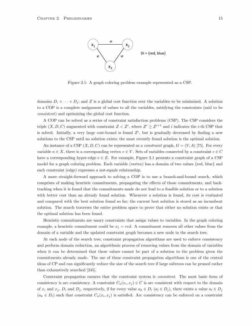
Chapter 2. Preliminaries 15
x1 x2
x3
≠
≠≠Di = red, blue
Figure 2.1: A graph coloring problem example represented as a CSP.
domains Di × · · · ×Dj ; and Z is a global cost function over the variables to be minimized. A solution
to a COP is a complete assignment of values to all the variables, satisfying the constraints (said to be
consistent) and optimizing the global cost function.
A COP can be solved as a series of constraint satisfaction problems (CSP). The CSP considers the
triple (X,D,C) augmented with constraint Z < Zi, where Zi ≥ Zi+1 and i indicates the i-th CSP that
is solved. Initially, a very large cost-bound is found Zi, but is gradually decreased by finding a new
solutions to the CSP until no solution exists; the most recently found solution is the optimal solution.
An instance of a CSP (X,D,C) can be represented as a constraint graph, G = (V,A) [75]. For every
variable n ∈ X, there is a corresponding vertex v ∈ V . Sets of variables connected by a constraint c ∈ Chave a corresponding hyper-edge e ∈ E. For example, Figure 2.1 presents a constraint graph of a CSP
model for a graph coloring problem. Each variable (vertex) has a domain of two values red, blue and
each constraint (edge) expresses a not-equals relationship.
A more straight-forward approach to solving a COP is to use a branch-and-bound search, which
comprises of making heuristic commitments, propagating the effects of those commitments, and back-
tracking when it is found that the commitments made do not lead to a feasible solution or to a solution
with better cost than an already found solution. Whenever a solution is found, its cost is evaluated
and compared with the best solution found so far; the current best solution is stored as an incumbent
solution. The search traverses the entire problem space to prove that either no solution exists or that
the optimal solution has been found.
Heuristic commitments are unary constraints that assign values to variables. In the graph coloring
example, a heuristic commitment could be x1 = red. A commitment removes all other values from the
domain of a variable and the updated constraint graph becomes a new node in the search tree.
At each node of the search tree, constraint propagation algorithms are used to enforce consistency
and perform domain reduction, an algorithmic process of removing values from the domain of variables
when it can be determined that these values cannot be part of a solution to the problem given the
commitments already made. The use of these constraint propagation algorithms is one of the central
ideas of CP and can significantly reduce the size of the search tree if large subtrees can be pruned rather
than exhaustively searched [245].
Constraint propagation ensures that the constraint system is consistent. The most basic form of
consistency is arc consistency. A constraint Cu(xi, xj) ∈ C is arc consistent with respect to the domain
of xi and xj , Di and Dj , respectively, if for every value ak ∈ Di (al ∈ Dj), there exists a value al ∈ Dj
(ak ∈ Di) such that constraint Cu(xi, xj) is satisfied. Arc consistency can be enforced on a constraint

Chapter 2. Preliminaries 16
by shrinking the domains of its variables. For example in the graph coloring problem, once x1 has been
assigned to red, constraint x1 6= x2 is no longer arc consistent because D1 = red, D2 = red, blue,but there does not exist any value in D1 that can support x2 = red while satisfying the not-equals
constraint. Therefore, the domain of D2 must be reduced to be D2 = blue to ensure arc consistency
of x1 6= x2.
In the graph coloring example, if only arc consistency is enforced on the binary constraints, no
reduction would be obtained at the root node. However, one can extend arc consistency to hyper-arc
consistency, also referred to as generalized arc consistency [215]. A constraint system is generalized arc-
consistent relative to constraint Cu(xi, . . . , xj) ∈ C if and only if for all variables xk, where k ∈ i, . . . , jand for every value ak ∈ Dk, there exists a tuple of values al ∈ Dl for all l ∈ i, . . . , j \ k such that
Cu(xi, . . . , xj) holds.
One type of constraint, called a global constraint, captures a relation between an arbitrary number
of variables and exploits problem sub-structures so that efficient propagation algorithms can be used to
perform domain reduction. For example, the AllDifferent global constraint is a constraint on a set of
variables x1, x2, . . . , xn, that imposes that each variable must take on a distinct value. Thus, one can
use the AllDifferent(x1, x2, x3) in place of the not-equals constraints in the graph coloring example and
improve propagation by enforcing generalized arc consistency. When the AllDifferent constraint is used,
the structure of the problem is taken into account and an inference algorithm based on the maximal
matching in a bipartite graph will recognize at the root node of the example problem that no feasible
solution exists since there are three vertices and only two distinct values in their domains [245].
After performing propagation, either heuristic search or backtracking is performed. If there are unas-
signed variables, none of which have an empty domain as a result of propagation, then a commitment will
again be made heuristically. This branching procedure leads to a new node where constraint propagation
can be performed again and search continues. However, if a variable is left with an empty domain, the
current node in the search tree has assigned one or more variables that cannot be part of any solution.
Thus, backtracking is performed and the node is pruned.
For scheduling problems in CP, a task is commonly modeled by a decision variable representing its
start time, sj , or completion time, cj . To ensure that tasks do not overlap, the disjunctive constraint
is used Disjunctive(s,p), where s, is a vector of start time decision variables and p are their processing
times [54]. However, variations on the Disjunctive constraint exists such as Cumulative, a more general
version that handles multi-capacity resources [5, 174]. For more details on the techniques used for
scheduling with CP, readers are referred to the book by Baptiste et a l. [20].
CP has been successful for scheduling problems [25, 118] including: nurse scheduling [195], business-
to-business meeting scheduling [196], robot task scheduling [47], and sports scheduling [153]. The ex-
pressiveness of CP and the performance of CP solvers for scheduling problems makes it an attractive
choice.
CP is used in Chapter 3 as a benchmarking technology and as the key component in the proposed
decomposition. The strengths and weaknesses of CP are explored to develop a decomposition that solves
two simpler problems using CP rather than solving the complete problem at once.

Chapter 2. Preliminaries 17
2.5 Decomposition Approaches
Rather than solving a complex problem altogether, decomposition approaches separate a problem into
smaller, more manageable parts to be solved and then appropriately combined. The aim is to have
decomposed problems that are more tractable and easier to understand than the complete problem.
This dissertation is focused on decomposition models and in this section a number of decompositions
are presented from the literature. Decompositions have been shown to be very useful for solving com-
plex scheduling problems and have therefore been heavily used [192]; thus, it is impossible to provide
a comprehensive review of decompositions given the large body of work. Following Raidl [202], three
decomposition approaches are described that build upon techniques coming from MIP: Lagrangian de-
composition, column generation, and logic-based Benders decomposition. The presentation of decompo-
sition approaches concludes with a review of ad-hoc decomposition methods designed to solve specific
scheduling problems.
It is possible to define many classification schemes to provide a framework for decompositions. For
example, one can define classification based on [202]: the techniques that are used, such as a MIP/CP
hybrid or one that makes use of two different metaheuristic algorithms; the level of hybridization based
on whether the algorithms used are weakly or strongly coupled; the order of execution of the decomposed
problems, which can be sequential, interleaved, or parallel ; or the control strategy being either integrative
or collaborative. Here, a classification scheme based on the type of problems that are generated by the
decomposition is used. The decomposed problems are either relaxed or restricted problems of the original
problem. Therefore, one can categorize each decomposition as either using a relaxation, a restriction, or
both.
Formally, a problem is a relaxation or a restriction based on the feasible region of the decision
variables, X = x1, x2, . . . , xn. Consider a subset of decision variables, X ⊆ X, which are the decision
variables for a problem partition of the decomposition. If the feasible region of X for the original problem
is defined as ΞX , and the feasible region of X for the partitioned problem as ΞX , then a relaxed problem
has ΞX ⊆ ΞX and a restricted problem has ΞX ⊆ ΞX .
A number of decompositions are presented in the remainder of this section. Three established de-
compositions are first described: Lagrangian decomposition, column generation, and logic-based Benders
decomposition. These decompositions represent a relaxed, restricted, and a mixed relaxed and restricted
decomposition, respectively. The section is concluded with a presentation of some ad-hoc decompositions
and a classification of each one within the proposed classification scheme.
2.5.1 Lagrangian Decomposition
Lagrangian relaxation is a method that produces an approximate solution to a linear programming
problem [89]. The method removes so-called complicating constraints and penalizes them in the objective
function rather than representing them as constraints. The aim is to obtain a relaxed model that can
be more easily solved than the original problem and provides a valid bound.
Given a linear programming problem,
max cTx (2.16)
s. t. Ax ≤ b. (2.17)
x ∈ X (2.18)

Chapter 2. Preliminaries 18
Once can split the constraints in A into a set of non-complicating constraints A1 ∈ Rm1,n, and compli-
cating constraints A2 ∈ Rm2,n. A relaxation of the problem can be defined as follows,
max cTx + λT (b2 −A2x) (2.19)
s. t. A1x ≤ b1. (2.20)
x ∈ X (2.21)
Here, λ = (λ1, λ2, . . . , λm2) are nonnegative weights, also known as Lagrange multipliers, that penalize
the violation of constraints in A2. The problem defined by (2.19) - (2.21) is called the Lagrangian
relaxation of the linear programming problem (2.16) - (2.18).
Once can show that the Lagrangian relaxation is an upper bound on the original problem for any
fixed set of λ values. Let x be the optimal solution to the original problem and let x be the optimal
solution to the Lagrangian relaxation. Since x is feasible in the original problem,
cT x ≤ cT x + λT (b2 −A2x), (2.22)
is true because λi values are nonnegative and (b2 −A2x) ≥ 0 for a feasible solution. Since x is optimal
for the Lagrangian relaxation, it can be shown that,
cT x + λT (b2 −A2x) ≤ cT x + λT (b2 −A2x). (2.23)
Therefore,
cT x ≤ cT x + λT (b2 −A2x), (2.24)
is true and the solution of the Lagrangian relaxation is a valid upper bound.
A Lagrangian decomposition, is a special case where the Lagrangian relaxation is decoupled into a
set of µ subproblems that can be independently solved. Consider the problem,
max cTx (2.25)
s. t. Ax ≤ b, (2.26)
Gx ≤ h, (2.27)
x ∈ X, (2.28)
where G is a mg×n constraint coefficient matrix and h is a vector of size mg. It is possible to reformulate
the problem as,
max cTx (2.29)
s. t. Ax ≤ b, (2.30)
Gy ≤ h, (2.31)
x = y, (2.32)
x ∈ X,y ∈ Y (2.33)
Chapter 2. Preliminaries 19
where y is a size n vector of decision variables and Y is a set containing X. The Lagrangian decomposition
consists of dualizing Constraint (2.32) with Lagrange multipliers λ. That is,
L(λ) := max(c− λ)x|Ax ≤ b,x ∈ X+ maxλy|Gy ≤ h,y ∈ Y. (2.34)
The Lagrangian dual is to find the Lagrange multipliers λ that result in the best bound,
minλL(λ). (2.35)
Lagrangian decompositions are a relaxation scheme. By representing hard constraints using a penalty
function in the objective, the feasible space of the Lagrangian relaxation contains all feasible solutions
to the original problem as well as infeasible solutions that would violate the constraint.
The Lagrangian relaxation can be used within a MIP branch-and-bound search by replacing the linear
programming relaxation to provide tighter bounds. This relaxation has been shown to be an effective in
a variety of scheduling applications such as: development of gas fields [107], flow shop scheduling [228],
job shop scheduling [138], and the unit commitment problem [261].
Decompositions exist that consider other solving techniques as aids to finding solutions of the La-
grangian relaxation, that is, Problem (2.35). For example, solving Lagrangian relaxations with meta-
heuristic methods to quickly obtain tight bounds can be beneficial. Cheng et al. [59] combine Lagrangian
relaxation and genetic algorithm by incorporating the latter as a method for updating the Lagrange mul-
tipliers. Similarly, Balci and Valenzuela [17] use particle swarm optimization in place of genetic algorithm
to search over the space of Lagrange multipliers in order to minimize the upper bound. These methods
are decompositions that help to improve the bound obtained by the Lagrangian relaxation without hav-
ing to perform an exhaustive search over all λ values. Although an exhaustive search might lead to a
better bound, it is often too costly to perform and the utility of an improved bound may not be worth
the higher computational effort.
In contrast to works that use decompositions to find solutions to Lagrangian relaxations, the bounds
found from the Lagrangian relaxations can be used to assist in finding the solutions of hard problems.
Bergman et al. make use of Lagrangian relaxations in CP [36] and multi-valued decision diagrams (MDD)
[37] to obtain improved lower bounds and apply the Lagrangian relaxation bound for cost-based domain
reduction. van den Heever et al. [243] develop a specialized heuristic algorithm that uses Lagrangian
decomposition by iteratively obtaining solutions to the Lagrangian relaxation as an upper bound and
postulates a feasible solution from the Lagrangian subproblems. These studies show the flexibility of
using Lagrangian decompositions within alternative search methods.
2.5.2 Column Generation
Column generation (also known as delayed column generation [76]) is an algorithm typically used for
solving problems where there are a large number of variables compared to the number of constraints.1
Column generation was first introduced to solve maximal multi-commodity network flows [91]. The
premise of column generation is to solve a restricted master problem where a subset of the variables
of the original problem are used. The algorithm is then to systematically add variables to the master
problem until an optimal solution can be found and proven.
1Although not all linear programs have significantly more variables than constraints, the Dantzig-Wolfe reformulationof a linear program can lead to an exponential increase in the number of variables [73].

Chapter 2. Preliminaries 20
The main idea behind of column generation is that all variables in a problem do not need to be
enumerated. For problems with an exponential number of variables, considering only a subset of the
variables can lead to significant reduction in computation effort. A key observation that provides intuition
into why column generation works is that the number of basis variables (non-zero variables) found when
solving the simplex method for a linear programming problem is equal to the number of constraints.
Therefore, even though the number of variables is large, only a small subset of these variables are part
of an optimal solution [40].
Consider the problem,
max cTx (2.36)
s. t. Ax = b, (2.37)
x ≥ 0, (2.38)
where x is a vector of size n representing the decision variables, c is a vector of size n, b is a vector of
size m, and A is a matrix of size m×n. Assume that the number of columns in matrix A is significantly
larger than the number of rows, that is, n >> m. Since only a subset of variables are necessary, one can
create a restricted master problem that considers the set of variables I, where |I| < n. The restricted
master problem is,
max∑i∈I
cixi (2.39)
s. t.∑i∈I
Aixi = b, (2.40)
x ≥ 0. (2.41)
A solution to the restricted master problem will be optimal for the set I, but can be sub-optimal
when the full set of variables is considered. To improve the solution, one must find a column (variable) to
enter the basis that is not in I and has negative reduced costs. If all variables not in I have non-negative
reduced costs, then introducing a variable to the restricted master problem will not improve the solution
and an optimal solution has been obtained.
The key to effectively solving column generation problems is in efficiently finding columns with
negative reduced cost or proving that none exist [40]. In general, determining that there does not exist
a column that can enter the basis is a hard problem. For example, solving the cutting stock problem
with column generation requires that a bin-packing sub-problem be solved to determine whether there
exists a column that can enter the basis [106]. Although this problem is still hard, it is computationally
cheaper than solving the original problem as the subproblem is often formulated in a way so that it can
be relatively easy to solve.
Column generation is a restricted decomposition scheme. The master problem is a restriction on the
solution space of a problem, where most of the columns have been removed. The subproblem is then to
search for a column of the original problem to reintroduce to the master problem. Therefore, column
generation starts with a very restricted master problem, but loosens this restriction after each iteration.
Column generation can significantly improve performance, but has the drawback of only solving
continuous linear programming problems. To guarantee that the solution obtained is optimal, it is
necessary to use the reduced cost of variables, which requires that decision variables be continuous.

Chapter 2. Preliminaries 21
Although one can round values to obtain an integer solution, it is not always guaranteed that the
resulting solution is optimal or even feasible. Therefore, branch-and-price is a method developed to
use column generation when some variables are restricted to be integers [22]. In this decomposition
framework, a branch-and-bound tree search is applied in which column generation is run at each node.
The use of column generation in scheduling problems has seen successes in a variety of applications
such as: nurse scheduling [21, 134], machine scheduling [58, 242], vehicle scheduling [209], and crew
scheduling [97]. For a more detailed survey on column generation and a listing of applications studied
with column generation approaches, see Lubbecke and Desrosiers’ survey paper [166].
2.5.3 Logic-Based Benders Decomposition
Logic-based Benders decomposition (LBBD) is a generalization of classical Benders decomposition [33]
developed by Hooker [125, 126, 127] to deal with combinatorial optimization problems by partitioning
the problem into a master problem and subproblem. LBBD iterates between solving the master problem
and subproblem, where solutions from the master problem are used to generate the subproblem and the
subproblem is used to determine cuts to be added into the master problem. LBBD differs from classical
Benders decomposition in that there are no structural restrictions on the different components of the
decomposition.
To model a problem for LBBD, the decision variables are first partitioned into two vectors x and y.
The problem to solve is then represented as,
min f(x, y) (2.42)
s. t. (x, y) ∈ Ω, (2.43)
x ∈ X, y ∈ Y. (2.44)
Here, f is a real-valued function, Ω is the feasible set (generally defined by a collection of constraints),
and X and Y are the domains of x and y, respectively. The problem partitioning is done to separate
the constraints into those involving only the x or master problem variables and constraints that have
both x and y, subproblem variables.
The master problem is formally defined as,
min z (2.45)
s. t. x ∈ Ω, (2.46)
z ≥ βxk(x), k = 1, . . . ,K (2.47)
x ∈ X, (2.48)
where z is a real-valued decision variable, Ω is a relaxation of Ω, and βxk(x) is a Benders cut on the
objective function f(x, y) found when fixing values of x to xk. Constraints (2.47) are obtained by solving
the subproblem and xi are solutions of the x variables found in the i-th iteration of the master problem.
The subproblem for iteration k is,
min f(xk, y) (2.49)
s. t. (xk, y) ∈ Ω, (2.50)

Chapter 2. Preliminaries 22
y ∈ Y. (2.51)
This problem is equivalent to the original problem, but with instantiated x variables based on the solution
of the master problem.
The LBBD algorithm iteratively solves the master problem and subproblem until convergence. The
master problem is solved to optimality, producing solution xk with cost zk in iteration k to be used to
formulate the subproblem, which then produces the bounding functions (that is, Benders cuts) on z. If
the k-th master problem solution satisfies all the bounding functions obtained in iteration 1 to k,2 the
process has converged to a globally optimal solution. Otherwise, the master problem must be solved
again and new Benders cuts are generated. Chu and Xia [61] show that LBBD converges to an optimal
solution in a finite number of iterations if the decision variables have finite domains and the following
two properties hold for the Benders cuts: 1) the cut must exclude the master problem solution if it is
not globally feasible, and 2) the cut must not remove any globally feasible solutions.
LBBD is a decomposition scheme that utilizes both a relaxation and a restriction. The master
problem is a relaxation since some constraints have been removed or relaxed. Thus, the resulting master
problem solution may not actually be valid and must therefore be tested in the subproblem. In contrast,
the subproblem is a restriction since the master problem has assigned the complicating x variables and
the subproblem solves for y given the assignment of x.
The use of LBBD has been successful in a number of scheduling applications such as: location/fleet
management [85, 86], queue design and control [232], maintenance planning and scheduling [9, 13], and
alternative resource scheduling [235]. These works generally consider MIP solvers for the master problem,
an exception being CP as an alternative [9, 232]. The subproblems of a LBBD are traditionally solved
using CP [126, 127], but studies have substituted other techniques such as MIP [9] and TSP [46, 235]
solvers.
In general, LBBD is a complete approach, but when problems are too large or complex to be solved to
optimality, an incomplete search can be considered. One simple method is to allow for an optimality gap
when solving the master problem [235]. The master problem can be too difficult to solve to optimality,
but finding good solutions within some acceptable bound may be easy. Therefore, one can search for
solutions until some optimality gap is proven and use the resulting solution to generate the subproblems.
Although the converged solution may not be optimal, the final solution will be bounded by the gap used
for the master problem.
Heuristics can also be used in place of the complete solver to obtain tractability. Cire et al. [62] use
a greedy heuristic that is enhanced with propagation techniques from CP to obtain solutions for the
master problem. They compare their incomplete LBBD model against regular LBBD and a pure CP
approach to show that the incomplete model can solve problems significantly larger than the other two
while also having equal or better solution quality.
Raidl et al. [203] take the use of incomplete methods further by applying a variable neighborhood
search for both the master problem and subproblem. They show that their method can solve problems
significantly larger than using classical LBBD. However, a later study by Raidl et al. [204] expanded
upon the previous model by performing a verification and correction step that employs a complete solver
when their approach has converged to ensure that incorrect cuts are removed and the master problem
has been solved to optimality. This extension makes the LBBD approach complete again, while still
2Note that the k-th master problem solution must also satisfy the bounding function generated by the subproblem ofthe k−th iteration.

Chapter 2. Preliminaries 23
benefiting from working through iterations faster. Their experimental results show that their approach
is able to find and prove optimality faster than LBBD.
2.5.4 Ad-Hoc Decompositions
The decompositions presented so far can be considered as formally defined frameworks that have each
been applied to a variety of problems. Here, some ad-hoc decompositions that makes use of heuristic
policies, MIP, and/or CP are discussed. Since a complete coverage of all ad-hoc decompositions is
impossible, this review will only provide a brief overview of some decompositions to illustrate the type
of approaches that can be found in the scheduling literature.
2.5.4.1 Incomplete Approaches
The first ad-hoc decomposition presented is the shifting bottleneck heuristic designed for job shop
scheduling problems [3]. The heuristic starts by solving a relaxation of the problem which ignores
resource constraints. A bottleneck machine is determined and a single machine scheduling problem is
solved for that machine to determine a job sequence. Based on this new schedule, the next bottleneck
machine is identified and solved. Once a schedule for the current bottleneck machine is determined, all
previously sequenced machines will be rescheduled one at a time, while also considering the previously
made sequencing commitments. The algorithm continues, scheduling each bottleneck machine until all
machines have been considered. The shifting bottleneck heuristic is both a relaxed and restricted de-
composition since an initial relaxation is used followed by progressive refinement of the schedule through
solving restricted single machine problems. Such a decomposition allows for the solving of a single
machine scheduling problem rather than the job shop scheduling problem, but loses the guarantee of
optimality.
Similar to the shifting bottleneck heuristic, which does not consider all machines at once, Wang and
Choi [254] decompose a multi-machine scheduling problem to solve only a subset of machines at a time.
They consider a flexible flow shop scheduling problem with machine breakdowns. Their decomposition
first makes use of a neighboring K-means clustering algorithm to group the machines based on their
stochastic nature due to machine breakdowns. A heuristic scheduler, either shortest processing time or
a genetic algorithm, is then used for each machine cluster to determine the sequence of jobs. The choice
of which scheduler to use is determined by a back propagation network [159], a commonly used artificial
neural network, to estimate the makespan difference of the schedules generated by the two schedulers.
Finally, the schedules from each of the machine clusters are integrated into an overall schedule. This
decomposition partitions the flow shop scheduling problem into smaller restricted problems to be solved.
Not only are the problems simpler, the clustering allows for a more appropriate scheduler to be chosen
to handle the stochastic nature of machine breakdowns.
An alternative approach to handling uncertainty in scheduling is to integrate classical scheduling
techniques with queueing theory models. Works by Terekhov et al. [233] and Tran et al. [237] propose
a two-stage decomposition for scheduling dynamic environments with flexible resources. Their works
make use of a queueing theoretic fluid model that solves a relaxation of the problem to provide long-
term guidance as to the stability conditions of a system.3 Using the solution of the fluid model as
guidance for how one should allocate jobs to machines in the long-term, a MIP [233] or LBBD [237]
3Stability here refers to the queueing theory notion whereby the throughput of the system is sufficient such that thequeues are guaranteed to not grow unboundedly over time.

Chapter 2. Preliminaries 24
model is then used to assign and sequence jobs online. The fluid model is a relaxation that only considers
the system dynamics by aggregating jobs and looking at a long-term scope of the system. The second
stage of assigning and sequencing jobs online can be thought of as a restriction since it uses a rolling
horizon to decide on the set of jobs to schedule and guides assignments based on the first stage solution.
Chapter 4 applies a similar approach of using a queueing theoretic fluid model to solve a relaxation of
the problem to provide long-term guidance.
2.5.4.2 Complete Approaches
The ad-hoc decompositions discussed so far are all incomplete approaches. However, optimality can be
important for many scheduling applications given that sub-optimal solutions can equate to large losses of
profit or to customer dissatisfaction. The remainder of this section is focused on complete decomposition
approaches.
Rasmussen and Trick [205] consider the timetable constrained distance minimization problem, a
sports scheduling problem for tournaments. The scheduler is tasked with finding optimal home-away
assignments for teams with respect to distance minimization given a schedule of when each team will
play one another. That is, for each game, the scheduler must decide the location of the game; either at
one team’s home location or the other’s. A MIP/CP hybrid is proposed for a two stage optimization
framework. In the first phase, CP is used to generate all feasible home-away patterns for each team in the
tournament. The second phase is to then assign each team to one of the generated patterns using MIP
in order to minimize the traveling distance. Here, CP works well for feasibility problems and is suited
for generating all possible home-away patterns. In contrast, MIP is found to work well for optimization
problems, which is required for the second phase. Within the proposed classification scheme, the pattern
generation can be thought of as a relaxation, since the set of patterns generated is a superset of actual
patterns, which is then used in the MIP model to solve the complete problem.
Techniques presented so far have been focused on partitioning a problem into two or more distinct
problems to be sequentially solved. Such a decomposition is useful when one can find intelligent and
meaningful ways to divide the decisions of a problem. For example, the decompositions discussed have
found appropriate ways to break their problems into simpler parts by: partitioning machines [3, 254],
separating the long-term and short-term decisions [233, 237], or generating patterns and then assigning
teams to these patterns [205]. However, one can also create a different style of decompositions, which
more tightly integrates two solvers in a hybrid algorithm, where the solution of one solver can assist in
solving another.
The probe backtracking algorithm [80] uses a linear programming (LP) subproblem solution to provide
search decisions for a CP solver. The CP model contains the original scheduling problem and the LP
model contains a linear representation of the activities and a cost function, but relaxes the resource
constraints. During CP search, the LP relaxation is solved at every node to provide a relaxed optimal
solution, which can either be a feasible solution or can be used to find time periods with over-utilization
of resources. Branches are made based on the sequencing of pairs of activities that have been identified
as problematic jobs based on the relaxed solution.
Beck and Refalo [31] extend the probe backtracking algorithm by identifying a cost relevant subprob-
lem (CRS) for the scheduling problem with earliness and tardiness costs. The CRS relaxes the problem
to only contain cost relevant activities; that is, the last activity of each job. If the resulting CRS solution
can be extended to a feasible solution, then it can be returned as the optimal solution for a subtree in

Chapter 2. Preliminaries 25
the CP search. Otherwise, the CRS solution can be used as a lower bound and the LP is solved as in
probe backtracking. These integrated approaches are shown to work well, since the relaxation of the
problem is not only relatively easy to solve and can sometimes be extended to complete solutions, but
is also useful for providing search guidance.
Ad-hoc decompositions can vary greatly to achieve different purposes. In Chapter 3, a decomposition
is used to solve simpler problems, which was seen in the works that partition machines to solve easier
problems [3, 254]. The work in Chapter 4 extends the queueing/scheduling hybrid works [233, 237] and
show the benefits of using tools from both combinatorial scheduling and queueing theory to complement
one another. Furthermore, the proposed queueing/scheduling hybrid follows the work by Rasmussen and
Trick [205] by using a pattern generating phase followed by an assignment to these patterns. Finally, a
tree search framework is used that is partially constructed and guided by a separate problem partition,
similar to i-STS and probe backtracking.
2.6 Summary
In this chapter, the background on scheduling and some common methodologies for solving scheduling
problems is presented. First, a brief background on common scheduling concepts is provided in Section
2.1, followed by a presentation of popular scheduling approaches. The presentation focused on method-
ologies relevant to the techniques that are employed in this dissertation: dispatch policies, MIP, and
CP. A review of the literature on decomposition approaches is then provided in Section 2.5. Specifi-
cally, three different decompositions are considered: Lagrangian decomposition, column generation, and
LBBD. Each decomposition is classified based on whether the partitions are a relaxation or a restriction
of the original problem. Finally, ad-hoc decomposition approaches are presented in Section 2.5.4, where
a number of incomplete and complete approaches were discussed.
Here, focus has been only on the scheduling approaches and not the literature on the application
problems or the work relevant for each chapter in this dissertation. Previous work related to each of the
individual contributions and application domain is presented in their respective chapters.

Chapter 3
Planning and Scheduling a Team of
Mobile Robots in a Retirement
Home4
3.1 Introduction
The recent aging of global populations is unprecedented in human history and it is not expected that
we will return to the younger population profiles of our ancestors [241]. The large increase in the
aged population has had, and will continue to have, profound impact on social and economic facets of
society. Of particular concern is the welfare and well-being of the elderly as their physical, cognitive,
and psychological requirements must be adequately met. However, without proportionately increasing
the number of professional caregivers, the increase of the older population will lead to a strain on the
existing system. To address the lack of human resources, human-robot interaction (HRI) and robot
companionship have been proposed and shown to have positive results on the human psychological state
[18, 240].
The work in this chapter is one part of a larger, long-term study of the deployment of intelligent
human-like mobile robots in retirement homes to assist and interact with the elderly residents [47, 162,
163, 165, 177]. The robot known as Tangy has been designed to: 1) navigate using a laser range finder
and 3D depth sensors, 2) detect users with 2D cameras, and 3) interact with users through speech,
gestures, and a touch screen. The proposed research problems include a myriad of technical challenges
with respect to robot hardware, control, sensing and intelligence. While the implementation of the
robot behaviors addresses robotics challenges, in this chapter the focus is on the global decision making
techniques which can plan and schedule the high-level tasks that a set of robots will perform during the
day in a retirement home. The decisions that must be made are what tasks to perform, where and when
to perform them, which residents are involved with these tasks, and which robot performs a particular
task. It is, of course, critical to take into account the personal preferences, schedules, and requirements
of each resident, creating a complex coordination problem where planned tasks must fit into the daily
4The work in this chapter is based on work published in the Journal of Artificial Intelligence Research [238]. Thiswork is in collaboration with Tiago Vaquero, who is responsible for the initial PDDL model (single-clock) presented in thischapter and was closely involved in the creation of the NDDL model. All other models were developed independently.
26

Chapter 3. Planning and Scheduling Mobile Robots in a Retirement Home 27
operations of a retirement home.
Due to external factors and uncertainties involved with human interaction, plans and schedules may
fail. However, replanning and rescheduling online are left for future work as obtaining a schedule first is
a crucial step towards implementation.
Planning and scheduling (P&S) is the joint problem of deciding what tasks to perform, when, and
with what resources, to achieve a set of goals. At the low-level, if a robot is given the goal of going
to a resident’s private room for a telepresence session, it has to plan a series of moves to navigate
from its current location to the resident’s room. In contrast, if a robot has requests for a number of
different tasks with different residents, it needs to schedule these tasks, taking into account the profiles
and preferences of the residents, the length of the tasks, and travel time between tasks. The focus here
is on this high-level P&S problem for two representative activities within the retirement home facility:
telepresence session and Bingo games. In the former, the robot autonomously navigates to the user in
his/her private room, prompts the user for a previously requested video call, starts the call and tracks
the user during the session. For the Bingo game, the robot autonomously finds and reminds participants
about the game prior to its start and then navigates to a specified location to conduct the game. During
Bingo, the robot acts as the game facilitator, calling out numbers, verifying Bingo cards, prompting
players to mark missed numbers and celebrating with winners. A centralized server will plan, schedule
and monitor the daily tasks of the robots while lower-level behaviors are planned and performed locally
by each individual robot [246].
This chapter has two primary aims: to study whether a particular robot planning and scheduling
application can be modeled and solved using current planning and scheduling technologies and to develop
a decomposition approach that provides daily robot task schedules with high user participation in social
activities. Such case studies serve as valuable feedback for researchers who focus on the theory and
algorithms which form the core of planning and scheduling research. As only off-the-shelf technology
is used, this work serves as a test of the extent to which the fields of domain-independent planning,
mixed-integer programming (MIP), and constraint programming (CP), are progressing toward the “holy
grail” [94] of declarative problem solving. While this test, focusing on a single application, is far from
definitive, it does provide a data point as to where we are in this quest as well as for the narrower goal
of solving similar planning and scheduling problems. The second goal of developing a decomposition
approach is important to ensure that it is possible to perform the daily global decision making required
for the implementation of the robots in a retirement home.
The main contributions of this chapter are:
• The modeling of a complex multi-robot HRI problem with four different solving technologies: AI
Planning, Timeline-Based Planning and Scheduling, MIP, and CP. Direct comparisons between
these technologies are uncommon as each formalism contains their own assumptions, restrictions,
and solving techniques that affect how one can and should develop a model.
• The development of a CP-based decomposition model that outperforms all other tested approaches.
Results for a proposed CP model provide insights on the short-comings of the technology to handle
some aspects of the robot tasks scheduling system; the decomposition presented takes into account
these problematic aspects by ignoring one of the complicating aspects of the problem in the first
stage, and then reducing the search space of the problem in the second stage by using the resulting
solution of the first stage, which allows a simplification of three other complicating aspects in order
to consistently obtain high quality solutions.

Chapter 3. Planning and Scheduling Mobile Robots in a Retirement Home 28
• The modeling and solving study of a complex temporal planning problem that lies at the intersec-
tion of planning and scheduling.
• An investigation of alternative models in Planning Domain Definition Language (PDDL) for timed
events and multi-user actions. The principles and practice of taking a real problem and developing
a model are not often discussed and alternative models tend to not be explored in depth in the
planning community. This work contributes to the study of effective modeling.
• The introduction of one of the first applications of CP to a multi-robot planning and schedul-
ing problem. Automated planning is commonly proposed for handling decision making in robot
systems. The results show that CP is a strong candidate with great potential to providing high
quality schedules.
• Identification of particular model components for PDDL planners (timed initial literals, tempo-
ral constraints, and complex objective functions) and CP solvers (massive numbers of optional
activities and complex objective functions) that are challenging for the technology.
The following section presents the details of the robot planning and scheduling application. Models
developed for the four technologies are outlined in Sections 3.3 to 3.6 followed by experimental results
comparing the different technologies in Section 3.7. Discussion of the results and future work directions
can be found in Section 3.8 followed by conclusions in Section 3.9.
3.2 Problem Description
The problem of interest is creating a daily schedule for multiple robots in a retirement home environment.
The main elements of the proposed problem are: the environment in which the residents (users) and
robots interact, the constraints, the goal and preferences. The constraints for the telepresence sessions
and Bingo activities were obtained from meetings with directors, healthcare professionals, and residents
from Toronto area retirement homes [162, 164]. The parameters and preferences used herein can be
changed as needed without a large impact on the models proposed in this chapter.
The Retirement Home Environment A floor in a retirement home is considered. The environment
consists of rooms and hallways that are discretized as a set of locations, L, within which the users and
robots interact. The distance between any two locations l and m, denoted dlm, is determined as part of
the discretization of the retirement home.
The Users The retirement home has a number of residents, represented by a set of users, U . Each
user, u ∈ U , has his or her own user profile consisting of a private room at a location in L, and a
schedule for the day. A user’s schedule provides the availability and location of the user from 7am to
7pm. During this time, the user may or may not be available for interaction with a robot: a user u
may be available between 10am and 11am at location l, but from 11am-12pm the same user can be at
location m and unavailable for any interaction. All users have meal breaks for breakfast (8am-9am),
lunch (12pm-1pm), and dinner (5pm-6pm), during which no user-robot interactions are possible. Each
user also has appointments during which no interaction can occur (e.g., art classes and family visits).

Chapter 3. Planning and Scheduling Mobile Robots in a Retirement Home 29
The user’s profile also contains his/her preference for a minimum, att minu, and maximum, att maxu,
number of Bingo games. Furthermore, some users may have telepresence sessions that have been booked
and must occur at some point during the day when the user is free.
The Robots The environment has a set of assistive robots, R, that are responsible for performing
the single-user activities (telepresence sessions) and multi-user activities (Bingo games). The robots also
provide users with reminders prior to any Bingo games that they are assigned to. To perform these
tasks, a robot must travel to the corresponding location (either the current location of the user or to the
games room for a Bingo game). Once the robot and user are together at the scheduled time, the robot
is then busy for the duration of the task and is not able to perform any other tasks.
While the robot is travelling and performing tasks, it consumes battery power at a rate dependent
on the task being executed. The battery level, bli, of robot i must always stay between bl mini ≤bli ≤ bl maxi. To ensure that a robot’s battery has sufficient energy, the robot can be scheduled to
recharge its battery up to bl maxi at a charging station. A constant recharging ratio of rri (V/min) is
used to approximate the recharging process of robot i. Although battery consumption and recharging
is non-linear, we consider a linear model to approximate the energy levels as a simplifying assumption.
A robot moves between locations at a constant velocity vi and so the estimated time to move from
a location l to m is dlmvi
. Moving consumes battery power with a constant rate of cr movei, the amount
of battery consumed for moving one unit of distance. Each HRI activity has a different rate at which
power is consumed: cr telepi, cr remindi, and cr Bingoi represent the consumption rate per minute of
a robot i for telepresence sessions, reminders, and Bingo activities, respectively. The robot must always
have sufficient battery power to return to a charging station.
Charging Stations A set of charging stations, K, is considered for this problem. Each station k ∈ Kis available in one of the locations and is able to recharge any of the robots. There can be any number of
charging stations per location. Each station has one docking spot and so can charge at most one robot
at a time. While a robot is docked, it cannot perform any other tasks. For a given level of charge, β,
that is desired after a charging action, the charging duration is CD(β) = β−blirri
.
Telepresence Sessions A set of telepresence sessions, S, is required to be scheduled during the day.
Each telepresence session y ∈ S is characterized by the user u, the location l (in the user’s private room),
the duration dury (30 minutes), and the time window (or multiple non-overlapping time windows) in
which the session may be held.
Bingo Games A set of Bingo games, G, is to be scheduled during the day. Bingo games are optional
activities that add value to the daily schedule for users. A Bingo game g ∈ G is characterized by the
location (i.e., the dedicated games room), the duration of the game durg (60 minutes), and the time
window (or multiple non-overlapping time windows) when it can be played. For each Bingo game g that
is played, the number of participants must be no less than p ming = 3 and no more than p maxg = 10.
These users must be available during the game and each player must be reminded of the game by a
robot 15 to 120 minutes before it begins. These times are chosen with the assumption that residents
may require up to 15 minutes to travel to the games room and that a reminder any longer than 120
minutes prior to the game may be forgotten. The robot that reminds a user does not need to be the
same robot that plays the Bingo game. The duration of a reminder is dur remindg (2 minutes) and can

Chapter 3. Planning and Scheduling Mobile Robots in a Retirement Home 30
Table 3.1: Distance between locations (meters).
Personal Personal Personal GamesRoom 1 Room 2 Room 3 Garden Room
Personal Room 1 0 25 25 50 25Personal Room 2 25 0 25 25 25Personal Room 3 25 25 0 25 25
Garden 50 25 25 0 25Games Room 25 25 25 25 0
Figure 3.1: Example user schedules. Blue tiles indicate when a user is busy with a personal activity, redtiles are meal times, green tiles represent the interruptible activities, and white tiles are leisure periodsof time when the users are in their own personal rooms and are available to interact with robots.
only be performed when a user is available. To remind a user, the robot must be in the same location
as that user.
The group of participants of a game is not known a priori. For a given game, the group of players
must be determined based on the residents’ schedules and attendance preferences.
Input and Goal The input of the problem is the sets of locations, L, users, U (with their profiles),
charging stations, K, available robots, R (with their initial locations, velocity, and battery level and
consumption details), and the requested telepresence sessions, S, and Bingo games, G, with their corre-
sponding properties. The goal is to create a plan of robot tasks in which all the requested telepresence
sessions are scheduled and the requested Bingo games and reminders are scheduled, if possible, given
that user attendance preferences have to be satisfied. All robots must be at a location with a charging
station at the end of the day. As a multi-objective optimization problem, the goal is to: 1) have as many
users playing Bingo as possible, 2) perform as many Bingo games as possible, 3) provide reminders as
close as possible to the game times, and 4) expend as little battery power as possible. More formally,
we wish to minimize the objective function:
f = 1000(|U | −#ofUserBingoParticiation) + 500(#ofGamesSkipped)
+ TotalDeliveryT ime+ TotalBatteryUsage. (3.1)
3.2.1 Simple Example Problem and Solution
Let us assume that there is a retirement home with five locations (rooms and travel times shown in
Table 3.1), three users (User1, User2, and User3), and two robots (Rob1 and Rob2). Figure 3.1 provides
the morning schedule of the users. Here, each user is willing to play in att minu = 0 or att maxu = 1
Bingo game during the times when they are available for interaction.
There is a single telepresence session and Bingo game to schedule, with time windows 7am - 10am

Chapter 3. Planning and Scheduling Mobile Robots in a Retirement Home 31
and 9am - 12pm, respectively. The telepresence session is thirty minutes in duration and is for User2.
Bingo games are played for one hour and must have at least three players. Reminders for Bingo games
take two minutes and must be performed between two hours and fifteen minutes before a Bingo game is
played.
The robots start the day (7am) in the Games Room where there is a single recharging station. Robots
are assumed to be at full battery capacity (100 units of battery power) at the start of the day and to
consume five units of battery power per minute of movement and one unit of battery power per minute
for all other tasks. The recharging rate of a robot is ten units of battery power per minute and they
travel at a velocity of five meters per minute.
A possible solution is to have the telepresence session for User2 performed from 7:05 to 7:35 and a
Bingo game at 11:00 that is played by all three users. This plan is embodied in a lower level plan as
follows:
Rob1
• Move from the “Games Room” to “Personal Room 2” at 7:00 to 7:05 - battery level at 75
• Perform telepresence session with User2 at 7:05 to 7:35 - battery level at 45
• Remind User2 at 9:58 to 10:00 - battery level at 43
• Move from “Personal Room 2” to “Games Room” at 10:00 to 10:05 - battery level at 18
• Recharge battery from 18 to 68 at 10:05 to 10:10 - battery level at 68
• Facilitate Bingo game with all three users at 11:00 to 12:00 - battery level at 8
• Recharge battery from 8 to 100 at 12:00 to 12:10 - battery level at 100
Rob2
• Move from the “Games Room” to “Personal Room 3” at 10:30 to 10:35 - battery level at 75
• Remind User3 at 10:38 to 10:40 - battery level at 73
• Move from “Personal Room 3” to “Personal Room 1” at 10:40 to 10:45 - battery level at 48
• Remind User1 at 10:45 to 10:47 - battery level at 46
• Move from “Personal Room 1” to “Games Room” at 10:47 to 10:52 - battery level at 21
• Recharge battery from 21 to 100 at 10:52 to 11:00 - battery level at 100
To calculate the objective value of the example solution, we show the value for each of the four
criteria: 1) three users participate in Bingo games; 2) one Bingo game is played; 3) delivery times are
15, 62, and 22 for User1, User2, and User3, respectively; and 4) energy usage is 151 and 79 for Rob1
and Rob2, respectively. Therefore, the total objective value is
f = 1000(3− 3) + 500(0) + (15 + 62 + 22) + (151 + 79) = 239. (3.2)
3.2.2 Problem Modifications
Various modifications to the problem are proposed to: 1) study how certain aspects of the problem affect
each of the proposed approaches, and 2) obtain better solutions through solving simplifications of the
original problem. The aim is to isolate particular properties of the problem that may prove to be difficult
to solve and thus to contribute insights into the strengths and weaknesses of the different technologies.
Five independent modifications are considered:
• B: battery. When the battery is removed from the problem, all aspects that have to do with
battery usage are ignored.

Chapter 3. Planning and Scheduling Mobile Robots in a Retirement Home 32
• R: reminder time windows. When removed, the reminders can be performed at any time prior to
the start of a Bingo game.
• P: participants. Bingo games may have a varying number of participants. When removed, the
assumption is that all games have exactly four players.
• O: optional Bingo games. This modification requires all Bingo games to be played.
• F: complex objective function. When removed, only user participation is considered and all other
objectives are ignored.
Each modification can be added or removed independently. The original problem is denoted as
BRPOF, where all aspects of the problem are considered. The problem where battery levels are ignored
and Bingo games are not optional is -RP-F. Since there are five independent properties, there are
25 combinations. Only a subset of these problems, which is believed to exhibit more interesting and
informative results, are looked at: BRPOF, -RPOF, B-POF, BR-OF, BRP-F, BRPO-, and B—F. These
problems represent the original problem, ones where each modification is made on its own, and the last
problem where the modifications regarding the Bingo game and reminders simplifies the Bingo game
properties.
Only BRPOF, BR-OF, BRP-F, and BRPO- provide sound solutions to the original problem. That
is, a feasible solution to any of these problems is also a feasible solution to the original problem. The
BR-OF, and BRP-F modifications can lead to infeasibility: no solution may exist with all Bingo games
played or with exactly four participants per game. In the scenarios tested, this is not the case and all
modifications have non-empty feasible regions. However, none of these modifications is complete: the
optimal solution of the original problem may not lie within the feasible region of the modified problem
or the optimal solution for the modified problem may not agree with the original problem. A solution
to -RPOF may result in a robot depleting its battery before completing all required tasks. B-POF and
B—F can lead to a solution where a user is reminded outside of the reminder window. Although this is
not as catastrophic as a depleted battery, the time windows were intended to be hard constraints. Tests
are performed for the models on problems -RPOF, B-POF, and B—F to observe how batteries and time
windows affect the solvability of the models, even though these models are not sound.
The solution of each problem instance by each approach is evaluated a posteriori using the original
objective function, which includes the presence of Bingo games, participation of users, delivery times,
and energy usage.
3.2.3 Task Representation in Planning and Scheduling
Each of the four formalisms of interest can be classified as either planning (PDDL and New Domain
Description Language (NDDL)) or scheduling (MIP and CP). While there are many differences be-
tween planning and scheduling, an important distinction is the abstraction used to model tasks in each
paradigm. In planning, it is sufficient to model tasks by utilizing operators, which dictate how the state
of the world may be changed. An operator is instantiated to create a ground action and the planner
decides how many times to instantiate each operator and their sequence to reach a goal state. For
example, to charge the battery on a robot, the planner has access to a battery recharging operator that
can be executed by any robot as many times as necessary.

Chapter 3. Planning and Scheduling Mobile Robots in a Retirement Home 33
Smith, Frank, and Jonsson [225] note that planning research has focused on problems where there are
tasks with cascading effects: a problem property where a decision regarding a task leads to requirements
for performing other tasks and making other decisions. More precisely, we are interested cascading
effects where the execution of a task leads to the required execution of one or more other tasks. We see
cascading effects in the robot scheduling problem from the Bingo games and reminders; for example, if
a Bingo game is played, then the number and identity of the players must be decided, triggering the
further need for reminders to be performed with specific residents. The flexibility of operators used in
planning is well suited to represent these cascading effects. In contrast, Smith, Frank, and Jonsson state
that scheduling is not well suited for tasks with cascading effects as it has focused on problems where
there is little task choice, but the resulting sequencing problem is harder. To represent cascading effects
in typical scheduling formalisms, every task and decision that might be required by other decisions must
be explicitly modelled and the scheduler must now also choose which, if any, of these tasks to perform
[148]. We note that this approach has its origins in the conditional constraint satisfaction problems
[176].
The general approach we take is to make use of optional tasks to model all the actions that the
planner may choose to instantiate. This approach allows one to model a task but not necessarily execute
it. For example, the maximum number of possible charging tasks must be known prior to scheduling in
order to know how many optional tasks to create. The same must be done for the reminders and Bingo
games since it is not known a priori which users are assigned to a Bingo game or whether a game will
be played or not.
The bounds introduced for the scheduling models provide the schedulers with additional information
not available to the planners. Although this added information can be useful for the scheduler to know
how many tasks it must consider, it may also hinder performance if the bound used is large as the
resulting problem instance may not be tractable.
Two bounds must be provided, the number of reminders and the number of recharges. Since it
is not known in advance which users will be assigned to each game, all possible assignments must be
considered. Therefore, it is necessary to model a reminder for each user for every game. Given that
there are |G| Bingo games and |U | users, there is at most a possibility of |G|× |U | reminders since a user
can only be reminded for each game at most once. For the recharging tasks, the scheduler is given the
choice to provide a recharging action between every non-charging action. Although it is unlikely that
any schedule will require a recharge that often, such a conservative approach is the most straight-forward
method to obtain a valid bound on the number of recharging actions. Therefore, given that there are
a possibility for |G| Bingo games,∑u∈U att maxu reminders, and |S| telepresence sessions, the total
number of recharging tasks instantiated for the scheduling models is |G|+ |S|+∑u∈U att maxu.
3.2.4 Related Work
Planning is a key component of intelligent behavior [104] and is primarily studied within Artificial
Intelligence (AI). While initiated in robotics [186], planning research has broad applications including
in autonomous rovers [98, 132], spacecraft and satellite control [93, 104, 207], clinical decision support
systems [87], and advanced manufacturing [250]. The algorithmic foundation of AI planning is state-
space search [104].
Scheduling is widely studied in both the AI and Operations Research communities [199]. The em-
phasis in the literature has been on the combinatorial nature of a problem and the development of

Chapter 3. Planning and Scheduling Mobile Robots in a Retirement Home 34
sophisticated optimization techniques. In general, robots have not received as much attention in the
constraint-based scheduling literature as they have in the planning literature. Namely, most scheduling
work focuses on robots in production lines [72, 139] and robot task scheduling [259, 260]. In these works,
all tasks must be processed and they do not lead to cascading effects on the actions of robots or require
reasoning about causation.
The integration of planning and scheduling has been investigated over the past several years in such
robotic applications as container transportation robots [7], office assistant robots [32], planetary rovers
[82], hospital assistant robots [194], and eldercare robots [56, 197]. In these applications, single robot
approaches are commonly studied.
With respect to HRI activities, existing work has mainly focused on automated reasoning about the
schedule of a single user. For example, the Pearl robot [197] uses the Autominder system [200] to reason
about an elderly person’s current and planned activities to determine if and when reminders should be
provided. The Autominder system has not been extended to consider multiple users. The Cobot robots
[66] plan and schedule HRI activities, including semi-autonomous telepresence sessions, and office tasks
based on requests from several users. However, the planning and scheduling are managed independently
and the user schedules are not considered as constraints on the robots’ tasks. Previous work studied a
similar system, but with a single robot and different restrictions on activities [47]. All HRI activities
in that work must be performed and the users associated to these activities are already known. In
this work, interaction activities are optional and the identity of individual users invited to participate
in group activities are decisions to be made. Although multiple user schedules have been considered in
other non-robotic scheduling and optimization applications (e.g., energy conservation in buildings, Kwak
et al. , 2012), in this work the focus is on problems in which it is required to reason about the schedules
of multiple users, limited resources, metric quantities, and both single- and multi-user HRI activities.
The research work here requires the combination of problem features that are often only individually
considered in the literature. It is important for such an application problem that these features, which
include optional activities, consideration of user schedules and preferences, and efficient deployment of
a fleet of robots, are addressed. Such a real world problem has not been studied before in the planning
and scheduling literature.
3.3 PDDL-based Planning
In order to test the capabilities of planners using PDDL [103] on the target problem, six different models
are tested. For clarity of the exposition, one model is presented in detail followed by the differences in
the other five models. PDDL code for the first model can be found in Appendix A.
It is important to distinguish the six different models and the seven problem modifications described
in Section 3.2.2. Each of the six models can be used to accurately and equivalently represent each of the
seven problem modifications. The only difference is in how aspects of the domain are represented. The
modeling strategies alter the representation of the problem in PDDL while the problem modifications
change the problem.
3.3.1 Domain Modeling
The itSIMPLE Knowledge Engineering tool [249, 248] is used to model the proposed problem. itSIM-
PLE follows an object-oriented modeling approach using Unified Modeling Language (UML) [189] and

Chapter 3. Planning and Scheduling Mobile Robots in a Retirement Home 35
<<agent>>Robot
ready : Booleanbl : Floatbl_min : Floatbl_max : Floatv : Floatcr_move: Floatcr_telep : Floatcr_remind : Floatcr_bingo : Floatrr : Floatact_done : Booleanplaying : BingoGame
move(from: Location, to: Location, cs: ChargingStation)do_telepresence(s: Telepresence, u: User, loc: Location, cs: ChargingStation)recharge(loc: Location, cs: ChargingStation)remind(u: User, g: BingoGame, loc: Location, cs: ChargingStation)skip_bingo(g: BingoGame)play_bingo(g: BingoGame, loc: Location, cs: ChargingStation)interact(g: BingoGame, u: User)
Location
MobileGamesRoom
Free : Boolean
User
Available : Booleannot_interactiong : BooleanRoom : Locationatt_min : Intatt_max : Intnot_assigned_game(g: BingoGame) : Booleanatt_num : Int
ChargingStation
Idle : Boolean
Activity
Free : Booleanmust_be_done : Boolean
not_done : Booleandone : Boolean
TelepresenceSession
local_user : Boolean
BingoGame
game_location : GamesRoomdur_remind : Intp_min : Intp_max : Intp_num : Intdelivery_time(u: User) : Floatp_cur : Int
<<utility>>Global
distance(l1: Location, l2: Location) : Int
distance_to_station(loc: Location, cs: ChargingStation) : Intgames_attendees : Intcan_start_clock : Booleancurrent_time : Floatdelivery_time_limit_max : Floatdelivery_time_limit_min : Floattotal_delivery_time : Floattotal_battery_usage : Floattotal_number_users : Intgames_skipped : Int
clock_ticker()
Figure 3.2: The UML Class Diagram of the first proposed problem model. Dashed lines represent aninheritance (e.g., Robot is a type of Mobile) and a solid line represents a relationship (e.g., a Mobile canbe at a Location).
generates a PDDL model. A UML diagram is presented in this section to help the reader visualize the
resulting PDDL model. Key PDDL action specifications are provided to illustrate the main transition,
state, resources, and temporal constraints in the model.
Object Types and Fluents. A visualization of the modeled object types (classes), fluents and op-
erators for the initial model variation is provided in the UML class diagram in Figure 3.2. The most
important classes are: Location, GamesRoom, ChargingStation, Robot, User, TelepresenceSession, Bin-
goGame and Global.
The Location and GamesRoom (a specialization of Location) represent the topology of the retirement
home. The distance between locations (distance), and the distance between each available charging
station and these locations (distance to station) are represented in the class Global. These two static
variables provide the distances in meters for every pair (location, location) and (location, station) in the
problem.
A games room is said to be free (fluent) when no game is taking place at the location. If a robot
is performing a task in the games room the fluent free is set to false. All the other locations have no
representation of their availability.
A ChargingStation is said to be idle (fluent) when no robot is docked for charging. In order to
represent the physical location of a station, the fluent available at is used to assign the station to a
particular location object.
The class User has a set of properties to represent the user’s location in the environment and the
user’s profile. The fluent at refers to the current location of the user who must be at one location at
a time. The static variable room specifies the user’s private room while the fluent available is used to

Chapter 3. Planning and Scheduling Mobile Robots in a Retirement Home 36
represent the availability of the user during the day. This availability is translated into PDDL in the
form of timed initial literals (TILs) [79] by assigning the available predicate to true or false in specific
time intervals. The known locations of the user during the day is also represented with TILs by assigning
the fluent at to the corresponding location based on the user’s activity locations. The user’s preferences
on attending games are represented by the fluents att min and att max. The fluent not assigned game is
used to list all the games to which a user has not yet been assigned, and the fluent participant to specify
the game to which the user has been assigned. The number of games planned for each user is written as
att num. Finally, when a user is interacting with a robot, the predicate not interacting is set to false to
prevent other robots from interacting with the same user.
The class Robot can also only be at (fluent) one location at a time and has all the properties (as
fluents) detailed in the problem description (e.g., velocity, battery level, etc.). In addition, the fluents
ready, act done, and playing are used. A robot is ready when it is not engaged in any tasks and it is
playing when it is performing a Bingo activity. The predicate act done prevents a robot from going to
a location and performing no action: a robot can only move to another location if it has completed a
task in its current location.
The classes TelepresenceSession and BingoGame represent the HRI activities that need to be per-
formed by the robots during the day. Both have the properties dur, to represent duration; not done and
done, to represent whether the task has been performed; and TILs must be done during, to represent the
time windows in which the task can be performed. In addition to the properties of the sessions and games
introduced in the problem description, the fluents p num and p cur are added to control the number
of users reminded by the robots and the number of users playing the game, as well as delivery time to
control the time each user is reminded about the game.
Modeling the separation time between the delivery of a reminder and its associated Bingo game is
done by using PDDL+ which includes processes [92]. A process (called clock ticker in the class Global)
models an exogenous activity that is triggered for as long as a condition holds (in this case the fluent
can start clock), regardless of the action selection process. This mechanism allows one to increment the
fluent current time one minute at a time, simulating the passage of time in discrete one-minute intervals.
If current time is used in an action’s precondition it will hold the exact start time of the action. This
variable is used to record the time each user is reminded (fluent delivery time) and also to check if the
start time of a game is within the time constraints of the reminders.
The class Global also holds global variables including the maximum and minimum time for deliv-
ering reminders prior to the games (fluents delivery time limit min and delivery time limit max ), the
total time generated by adding all the lengths of the time intervals between the reminders and the
game (fluent total delivery time), the total amount of battery power consumed by all robots (fluent to-
tal battery usage), the total number of games not played (fluent game skipped), the total number of users
attending games (game attendees) and the number of target users (total number users). These variables
are used to specify the cost function and are manipulated in the specification of the robot actions.
Operators. As shown in Figure 3.2, a robot has the following operators:
• move to a location
• recharge its battery
• remind a user

Chapter 3. Planning and Scheduling Mobile Robots in a Retirement Home 37
• do telepresence with a user
• play Bingo with a group of users
• interact with a player during the Bingo game
• skip Bingo which removes the game from the request list.
Here, the operators related to the Bingo activity are shown given its modeling complexity. For the
complete PDDL model, see Appendix A.
In the remind operator, a robot must be ready to perform the task and the user has to be available
at the same location as the robot. As an effect of the operator, the user is set as a participant of the
game. The time of the reminder is recorded in the fluent delivery time, which will become a constraint
(condition) for the Bingo operators. The remind operator is also used to increase p num and att num, the
number of users participating in a game and the number of games the user participates in, respectively.
The remind operator is defined as follows:
(:durative-action remind
:parameters (?self - Robot ?u - User ?g - BingoGame ?loc - Location
?cs - ChargingStation)
:duration (= ?duration (dur_remind ?g))
:condition
(and
(over all (at ?self ?loc))
(over all (at ?u ?loc))
(over all (available ?u))
(at start (ready ?self))
(at start (at ?self ?loc))
(at start (at ?u ?loc))
(at start (available ?u))
(at start (not_interacting ?u))
(at start (not_done ?g))
(at start (< (p_num ?g) (p_max ?g)))
(at start (not_assigned_game ?u ?g))
(at start (< (att_num ?u) (att_max ?u)))
(at start (>= (bl ?self) (+ (+ (* (dur_remind ?g)
(cr_remind ?self)) (* (distance_to_station ?loc ?cs)
(cr_move ?self))) (bl_min ?self))))
)
:effect
(and
(at start (not (ready ?self)))
(at start (not (not_interacting ?u)))
(at end (ready ?self))
(at end (not_interacting ?u))
(at start (increase (p_num ?g) 1))

Chapter 3. Planning and Scheduling Mobile Robots in a Retirement Home 38
(at start (participant ?g ?u))
(at start (not (not_assigned_game ?u ?g)))
(at start (increase (att_num ?u) 1))
(at end (act_done ?self))
(at start (decrease (bl ?self) (* (dur_remind ?g)
(cr_remind ?self))))
(at start (assign (delivery_time ?g ?u) (current_time)))
(at start (increase (total_battery_usage)
(* (dur_remind ?g) (cr_remind ?self))))))
Below, the play Bingo and interact operators are presented together. In order to play a game after
the reminders, a robot has to first start the play Bingo action, then it has to concurrently perform
the interact action with each participant. The play Bingo action requires that the number of players
that have been reminded, p num, is within p min and p max. Furthermore, p cur, also accounts for
the number of users participating in a Bingo game and is increased through the interact operator. The
requirement that p num = p max ensures that the correct number of users that have been reminded of
a Bingo game, also play the Bingo game. Together with the precondition of interact that requires a user
to be playing a game, the correct users that were assigned to a game through reminders will play the
Bingo game.
(:durative-action play_Bingo
:parameters (?self - Robot ?g - BingoGame ?loc - GamesRoom
?cs - ChargingStation)
:duration (= ?duration (dur ?g))
:condition
(and
(at start (at ?self ?loc))
(over all (at ?self ?loc))
(at start (ready ?self))
(at start (must_be_done_during ?g))
(over all (must_be_done_during ?g))
(at start (game_location ?g ?loc))
(at start (not_done ?g))
(at start (<= (p_num ?g) (p_max ?g)))
(at start (> (p_num ?g) (- (p_min ?g) 1)))
(at end (= (p_cur ?g) (p_num ?g)))
(at start (>= (bl ?self) (+ (+ (* (dur ?g) (cr_Bingo ?self))
(* (distance_to_station ?loc ?cs) (cr_move ?self)))
(bl_min ?self))))
(at start (free ?loc)))
:effect
(and
(at start (not (ready ?self)))
(at end (ready ?self))
(at end (done ?g))

Chapter 3. Planning and Scheduling Mobile Robots in a Retirement Home 39
(at start (not (not_done ?g)))
(at start (playing ?self ?g))
(at end (not (playing ?self ?g)))
(at end (act_done ?self))
(at start (decrease (bl ?self) (* (dur ?g) (cr_Bingo ?self))))
(at start (increase (total_battery_usage) (* (dur ?g)
(cr_Bingo ?self))))
(at start (increase (games_attendees) (p_num ?g)))
(at start (not (free ?loc)))
(at end (free ?loc))))
(:durative-action interact
:parameters (?self - Robot ?g - BingoGame ?u - User)
:duration (= ?duration (- (dur ?g) 1))
:condition
(and
(at start (playing ?self ?g))
(over all (playing ?self ?g))
(at start (available ?u))
(over all (available ?u))
(at start (not_interacting ?u))
(at start (participant ?g ?u))
(at start (>= (delivery_time_limit_max)
(- (current_time) (delivery_time ?g ?u))))
(at start (<= (delivery_time_limit_min)
(- (current_time) (delivery_time ?g ?u)))))
:effect
(and
(at start (increase (p_cur ?g) 1))
(at start (not (not_interacting ?u)))
(at end (not_interacting ?u))
(at start (increase (total_delivery_time)
(- (current_time) (delivery_time ?g ?u))))))
The passage of time in this model is managed through the PDDL+ process called clock ticker. The
process gets updated in every tick of the planner’s clock in increments of one minute.
(:process clock_ticker
:parameters ()
:precondition
(can_start_clock)
:effect
(increase (current_time) (* #t 1.0)))

Chapter 3. Planning and Scheduling Mobile Robots in a Retirement Home 40
Goal and Objective Function. In the goal state, all sessions and games must be done (Bingo games
can be either performed or skipped) and the user preferences on game attendance must be satisfied. The
aim is to minimize the following weighted cost function f :
f = 500(games skipped) + 1000(total number users− games attendees)
+ total delivery time+ total battery usage, (3.3)
where the weights are used to express preference on optimizing the number of games and players. In
PDDL this cost function is represented as follows:
(:metric minimize
(+ (* 500 (games_skipped))
(* 1000 (- (total_number_users) (games_attendees)))
(total_battery_usage)
(total_delivery_time)))
3.3.2 Alternative Modeling Strategies
The modeling possibilities for the target problem are numerous. Modeling strategies that result in
five additional PDDL models are now presented. Requirements that are more complicated to model
intuitively and efficiently in PDDL are presented: the Bingo game activity requirements on the robot’s
interaction with participants and the constraint on the temporal separation between reminders and
Bingo games. Essentially, the representation of these two aspects of the problem is changed to obtain
the alternative PDDL models. Altogether, three strategies for the first aspect and two for the second
are proposed, resulting in six different models.
User-Bingo Interactions In the initial model, users play Bingo games through the interact opera-
tion that is performed concurrently with the play Bingo operation in order to individually model user
interactions with the robot in the multi-user activity. This strategy is denoted as single, since single
users are considered for interaction. Two alternative strategies are presented that aim to explicitly
model interactions with users in the play Bingo operator. If it is assumed that there are exactly three
participants, the operator play Bingo3 may be defined as shown in Appendix A. The preconditions and
effects of this operator are an amalgamation of the play Bingo and interact operators to include the user
interactions in the play Bingo operator. To improve the model further, symmetry breaking is used in
the precondition (i.e., user i has I.D. less than user i+ 1) to reduce the available permutations.
As mentioned, two alternatives are proposed to handle the user-Bingo interactions: set-all and min-
add. The first, set-all, removes both the play Bingo and interact operators and uses multiple play BingoX
operators where X is between 3 and 10 to account for all possible number of participants in a Bingo
game. Essentially, this strategy sets all the participants in a Bingo game in the play Bingo action.
However, the number of participants is not known in advance, multiple operators with varying numbers
of users are required. The second strategy, min-add is a combination of the two strategies that will
only replace play Bingo by play Bingo3. By doing so, the Bingo games will start with the minimum
number of players and then increase participation through interact actions with other users to add more
players than the allowed minimum. The min-add strategy is therefore a combination of single and set-all

Chapter 3. Planning and Scheduling Mobile Robots in a Retirement Home 41
Bingo_overall
reminder
reminder
setup_Bingo
play_Bingo
interact
interact
Time
Figure 3.3: Example of a Bingo game with two participants. The Bingo overall action encompassesall reminder, setup Bingo, play Bingo, and interact actions associated with the Bingo game. Here, thesetup Bingo action separates the reminders and the Bingo game to ensure that a minimum amount oftime has passed. The length of the Bingo overall action ensures that the separation of the remindersand the Bingo game is less than the maximum allowed time. An intuitive representation of the influenceof the preconditions and effects of each action is provided through the use of precedence relationships(arrows) showing the relative ordering of actions.
by using the play Bingo3 action to play a Bingo game with three users and potentially adding more
participants using the interact action.
Reminder Delivery The current model makes use of the process clock ticker to keep track of the
time passed between a reminder and a Bingo game. This strategy is denoted as clock. The proposed
alternative, envelope is to make use of an encompassing larger action, Bingo overall (detailed in Appendix
A), that executes over all the Bingo related actions and must occur while any remind, play Bingo, and
interact actions are being executed (see Figure 3.3). This action spans all those actions to ensure the
timing constraints are met. By setting the envelope action to be the appropriate duration (maximum
delivery time plus duration of a Bingo game), a reminder cannot be separated from a Bingo game by
more than the maximum delivery time. To ensure that reminders do not occur too close to a Bingo
game, a new operator, setup Bingo, is introduced with duration equal to the minimum separation time,
which must occur between reminders and the Bingo game.
To use the proposed alternative strategy, new fluents are introduced. Each game can either be
Bingo actions ready or Bingo actions not ready based on whether Bingo overall is being executed and
any actions related to a Bingo game (remind, play Bingo, and interact) has a prerequisite that a Bingo
game has the fluent Bingo actions ready set as true. A fluent, Bingo game ready, is also required to
enable the start of a Bingo game after setup Bingo has been performed. Finally, a remind enable fluent
is used to state when users can be reminded or not.
The remind operator is updated to require remind enable to be true as a precondition and the
play Bingo requires Bingo game ready to be true. The setup Bingo operator is presented in Appendix
A.
Alternative Models The strategies proposed for both the user-Bingo interactions and the delivery
time window constraints can be applied independently, resulting in six different models. One of the six
models was already shown with single interaction actions being the sole method for users to play in

Chapter 3. Planning and Scheduling Mobile Robots in a Retirement Home 42
Bingo games and the use of processes to enforce separation constraints, single-clock. Table 3.2 presents
an overview of the six models and the strategies they use.
Table 3.2: Alternative Models
User-Bingo Interaction Reminder DeliveryClock Processes Envelope
Single Interactions single-clock single-envelopeSet Min Then Add min-add-clock min-add-envelope
Set All Players set-all-clock set-all-envelope
3.3.3 Problem Modifications
The PDDL models discussed above correspond to the BRPOF problem definition. Here, the updates to
the PDDL model to handle each of the five different modifications, B, R, P, O, and F is shown.
B: Battery The removal of battery constraints in the model is straightforward. All fluents related to
the battery are removed, specifically bl, bl min, and bl max. Any preconditions and effects that relate
to any of these fluents are also removed so that the battery is no longer considered. In addition, the
recharge operator is deleted from the model and the objective function is simplified to remove the battery
component. These changes can be performed on all of the six models identically.
R: Remove Separation Constraints To handle the modification R, time constraints on the delivery
time must be relaxed such that reminding a user at any time before a Bingo game is sufficient. To
make this change, delivery time limit min and delivery time limit max must be updated to 0 and H,
respectively, where H is the planning horizon minus the duration of a Bingo game. In the models that
make use of clock ticker, the separation time constraint in the precondition of play Bingo and interact
actions will change accordingly depending on the model. The models with the Bingo overall operator
will increase the duration of this action to extend over the entire planning horizon and will also remove
the setup Bingo operator. Since the setup Bingo operator is no longer used, the fluent Bingo game ready
is removed and a delete effect is added to play Bingo to remove enable remind to ensure that reminders
still must occur before Bingo games.
P: Set Number of Participants The models must be treated differently to ensure that exactly four
users participate in any game that is played. For the two models single-clock and single-envelope, p min
= p max = 4 is set to force the planner to only consider plans where four interact actions are used for
each Bingo game. The remaining four models will make use of only play Bingo4 operator and remove
any other play Bingo and/or interact operators.
O: Bingo Games are No Longer Optional It is ensured that all games are played by removing the
skip bingo operator. The objective function can be simplified to remove the games skipped component
since all games will be played. This change can be done for all six models.

Chapter 3. Planning and Scheduling Mobile Robots in a Retirement Home 43
F: Simplified Objective Finally, for modification F, one must only consider user participation of
Bingo games in the objective. Furthermore, for the three models that use the Bingo overall task to
model the constraint on the separation time, the removal of the exact separation time required for use
in the objective function means that it is possible to remove the clock processes entirely.
3.3.4 Modeling Issues and Limitations
An important challenge in modeling the problem in PDDL is dealing with time constraints between
actions (i.e., time delays between reminder and Bingo games). To be able to model time constraints, one
must model a clock as a process that is constantly incremented or make use of the larger encompassing
task with required concurrency. If processes are used, the start times of reminder activities must be
marked and used to restrict the precondition of the Bingo games. Doing so allows the solver to verify
that the two tasks are temporally consistent. However, few planners are able to handle this clock/process
approach, limiting the solvers that can be used.
Another issue is the flexibility in the number of participants of a Bingo game. In general, PDDL has
the tools to model the Bingo attendees as a decision variable through the use of the feature forall, but
the planners that are tested do not seem to support forall along with other features that are needed
(e.g., numeric, temporal, optimization, etc.). Due to this limitation, two alternative approaches are used:
1) required concurrency in which there is an action play bingo that is a container for each individual
interaction with a user and a robot, and 2) multiple duplicates of a single Bingo game, play BingoX, one
for each possible number of participants, X, in a game.
Finally, current STRIPS planners, in general, do not handle negative literals in preconditions. This
limitation leads to substantial redundancy as many not predicates must be used to represent these
negative preconditions.
3.4 Timeline-based Planning and Scheduling
Timeline-based planning and scheduling differs from action-based planning as it represents the world in
terms of a set of functions of time that describe how the world changes over a temporal interval [57].
The Extensible Universal Remote Operations Planning Architecture (EUROPA) system is a class
library and tool set developed at the National Aeronautics and Space Administration (NASA) for build-
ing timeline-based planners and schedulers [23]. EUROPA represents a technology that appears to be
a good fit for solving the problem of interest. Thus, this technology is a potential candidate to be
explored. However, during the investigation of EUROPA, it was learned that the solver was not made
to fit within the model-and-solve paradigm that is pursued here, but rather requires customization to
fit the particular application.
EUROPA uses New Domain Definition Language (NDDL) as the main input modeling language
[23]. Like PDDL, NDDL uses state and activity descriptions. However, NDDL state variables are called
timelines, temporally extended predicates that can be in a single state at any instant in time.
NDDL is object-oriented and can represent most physical entities within the retirement home as
objects. Figure 3.4 is the UML class diagram for the NDDL model. The objects used are very similar
to those used in the PDDL model and so fewer details are presented regarding each individual class, but
the major difference between the PDDL and NDDL models are emphasized: the addition of timelines

Chapter 3. Planning and Scheduling Mobile Robots in a Retirement Home 44
User
Timelines
UserState :
UserAvailability :
UserGameAssignment :
<<agent>>
Robot
Battery : Reservoir
Actions
move(p : Path)
RechargeBattery(cs : ChargingStation)
DoTelepresence(s : TelepresenceSession, u : User)
PlayBingo(g : BingoGame, gr : GamesRoom, u1 :
User, u2 : User, …)
Remind(g : BingoGame, u : User)
Timelines
RobotState:
Location
Mobile
GamesRoom
GamesRoomUsage :
Reusable
ChargingStation
charging_station : Location
ChargingStationUsage :
Reusable
Activity
loc : Location
dur : Int
TelepresenceSession
LocalUser : User
Timelines
TelepresenceSessionState :
BingoGame
players : Int
Timelines
BingoGameState :
Path
from : Location
to : Location
distance : Float
ChargeFree
AtMove PlayTele Rem
Play.At Interact. Rem.
Available Busy
Assigned.Not
Assigned
Being
Assigned
Done.Must Be
Done
In
Progress
Done.Must Be
Done
In
Progress
Figure 3.4: The UML Class Diagram of the proposed EUROPA model. Dashed lines represent aninheritance (e.g., Robot is a type of Mobile) and a solid line represents a relationship (e.g., a Mobile canbe at a Location).
and resources (reusable and reservoir) as first-class objects. The NDDL model is discussed here at a
high-level; the encoding can be found in Appendix B.
The Environment Various classes are used to represent the static environment of the retirement
home. Each of the rooms is an instance of a Location class and two such instances are linked together
by a Path which defines the distance between any two locations. A location may have a ChargingStation
that is represented as a reusable resource, ChargingStationUsage, to model the availability of the station
over time.
Activities Telepresence sessions and Bingo games are also represented with classes. Each telepresence
session is associated with a particular user, location, and duration and has the timeline Telepresence-
SessionState to indicate its state. The timeline has three values: MustBeDone, InProgress, and Done.
At the beginning of the day, the state of the telepresence session is MustBeDone, indicating that the
telepresence session has not yet been performed. Once a robot starts the action DoTelepresence, the
TelepresenceSessionState timeline changes to InProgress. Upon completion of the telepresence session,
the state changes to Done.
Bingo games have a particular location, duration and number of players associated with them. Similar
to the set-all modeling strategy used for PDDL planning, the number of players is prescribed in the
timeline-based model as a fixed value for the Bingo games. See Section 3.4.1 for details. Each Bingo
game, like a telepresence session, has a timeline, BingoGameState, indicating the state of the Bingo
game.
Recall that each activity has one or more time windows in which the activity can be performed.

Chapter 3. Planning and Scheduling Mobile Robots in a Retirement Home 45
These time windows are represented in the declaration of the initial state to indicate when the activity
can be performed, similar to the representation of the user schedules.
Users Users are represented by a User class. Each user has three associated timelines: UserState,
UserAvailability, and UserGameAssignment. The UserState defines the state of the user, which can
be either At, Interacting, Playing, or BeingReminded. While the user is not engaged with a robot,
the UserState will be in the At(l) state, which is a parameterized state which indicates that the user
is at location l. Interacting, Playing, and BeingReminded are states indicating that the user is in a
telepresence session, playing a Bingo game, and being reminded, respectively. The UserAvailability
timeline indicates whether the user is Busy or Available. During the time a user is interacting with a
robot or is at an appointment as per his/her personal schedule, the UserAvailability is Busy. The final
user based timeline is UserGameAssignment which has three states: NotAssigned, BeingAssigned, and
Assigned. Every user starts as NotAssigned and once a robot reminds a user, UserGameAssignment
transitions to BeingAssigned. Upon playing a Bingo game, the UserGameAssignment will change to
Assigned to indicate that the player has been assigned to and played in a game.
Robots Robots are represented by a Robot class. Each robot has a RobotState timeline that indicates
the state of the robot: FreeAt, Moving, Charging, DoingTelepresence, PlayingGame, and Reminding.
Each robot also has a Battery resource, which is represented using a reservoir that can be consumed or
replenished.
Robots have five actions: Move, RechargeBattery, DoTelepresence, PlayBingo, and Remind. Each
action requires timelines to be in particular states and changes the state of the timelines. For example,
Move changes the location of a robot from the current location to the destination location indicated
in the Move action. Move requires the use of a Path between the current location and the destination
location which provides the distance the robot must move, and therefore the duration of the movement
and the battery usage. The modeling of the Bingo related tasks in NDDL follows the same strategy as
the set-all strategy of the PDDL models by handling all participation within the PlayBingo operator.
3.4.1 Modeling Issues and Limitations
All aspects of the environment could not be fully represented using EUROPA since the initial goal was
to model and solve the problem without changing the solver code. While EUROPA is a very flexible
and expressive package, significant effort and deeper knowledge is required to represent more complex
components of the system.
The number of participants in a Bingo game is difficult to model since participating users must be
connected to the game. By leaving the number of users as a decision variable, it was not possible to
model which users were playing the games, while also ensuring that the number of participants in a
game is within the required bounds. By fixing the number of users in a game to an appropriate size, the
interaction of users playing in Bingo games can be modeled and the provided bounds on the number of
participants are ignored.
Furthermore, an objective function could not be represented. Although it is possible in EUROPA to
optimize, it requires altering the solver. EUROPA has built-in backtracking, but the backtracking rules
and decision procedure must be coded to perform any optimization. Otherwise, EUROPA will return
to a prior state by backtracking, but continue to make the same decision leading back to the state the

Chapter 3. Planning and Scheduling Mobile Robots in a Retirement Home 46
system was in prior to backtracking. Without an objective function that allows the solver to reason
about the optional Bingo games, Bingo games must be represented like the telepresence sessions and
made to be mandatory; otherwise, Bingo games will not be played and only the telepresence sessions
will be performed.
EUROPA leaves open many possibilities for those wishing to use timelines in their planning and
scheduling problems. However, this flexibility comes at the cost of a more involved process while writing
the code for modeling and solving the problem. Due to the requirement of a deeper understanding of
the EUROPA architecture and code to extend the solver to fully express the problem, the scope of the
problem represented by timeline-based planning and scheduling is limited in this study. Unfortunately,
at this time, no solver exists that can handle NDDL in the model-and-solve approach.
Another modeling language using a timeline approach, Action Notation Modeling Language (ANML),
aims to combine strong notions of action and state (from PDDL), a variable/value model (from NDDL),
and rich temporal constraints (from NDDL) [224]. However, the investigation into ANML and the FAPE
solver [78] led to the conclusion that, like NDDL, ANML is a good fit for representing the problem, but
the FAPE solver has not yet been implemented with the necessary features to solve the problem.5
Therefore, this work does not study ANML any further.
3.5 Mixed-Integer Programming
A MIP model is introduced to handle the robot task scheduling problem. Below the full set of decision
variables and parameters relevant for the MIP model are defined.
Decision Variables:
wj : 1 if a task j is scheduled and 0 otherwise,
xij : 1 if a task j is scheduled to be processed by robot i and 0 otherwise,
yjt: 1 if task j is scheduled to start at time t and 0 otherwise,
zijj′ : 1 if task j starts directly before task j′ on robot i and 0 otherwise,
φujj′ : 1 if task j is sequenced at some point before task j′ for user u and 0 otherwise,
δgu: delivery time for the reminder to user u in game g. If user does not play in game g, δgu = 0,
Bj : completion time of task j,
Ej : energy level of the robot that processes task j at the time of completion for task j,
Dj : duration of a job j,
ej : energy consumed by a job j.
5Filip Dvorak, personal communication.

Chapter 3. Planning and Scheduling Mobile Robots in a Retirement Home 47
Input Parameters:
R: set of robots,
U : set of users,
K: set of charging stations,
S: set of telepresence activities,
G: set of Bingo game activities,
M : set of reminder tasks,
Mg: set of reminder tasks corresponding to Bingo game g,
Mu: set of reminder tasks corresponding to user u,
Mgu: set of reminder tasks corresponding to user u and Bingo game g,
C: set of charging tasks,
CSk: set of charging tasks corresponding to charging station k,
A: set of all tasks A = S ∪G ∪M ∪ C,
Au: subset of tasks in A that involves user u,
a: an auxiliary task signifying the start of a schedule,
a: an auxiliary task signifying the end of a schedule,
A: set of all tasks including both auxiliary tasks A = A ∪ a ∪ a,Au: set of tasks that involve user u and the auxiliary tasks Au = Au ∪ a ∪ a,Tj : set of time points where task j can start,
Tgu: set of time points where a game g can start if user u plays,
T : set of all time points in the scheduling horizon,
θj : duration of task j, j ∈ A \ C,
V : a large positive number.
The MIP model proposed is presented below.
min∑j∈G
1000 ∗ (|U | −∑j∈M
wj) + 500(1− wj) +∑u∈U
∑g∈G
δgu −∑
j∈A\C
ej (3.4)
s.t. wj = 1 ∀j ∈ S ∪ a ∪ a (3.5)∑j∈Mgu
wj ≤ wg ∀u ∈ U, g ∈ G (3.6)
∑i∈R
xij = wj ∀j ∈ A (3.7)∑t∈Tj
yjt = wj ∀j ∈ A (3.8)
∑j∈A∪a
zijj′ = xij ∀j′ ∈ A ∪ a, i ∈ R (3.9)
xij′ + xij ≥ 2zijj′ ∀j, j′ ∈ A, i ∈ R (3.10)∑i∈R
∑j∈A∪a
zijj′ = wj ∀j′ ∈ A (3.11)
xij = 1 ∀i ∈ R, j ∈ a ∪ a (3.12)

Chapter 3. Planning and Scheduling Mobile Robots in a Retirement Home 48
∑j∈Mg
wj ≤ p maxg ∀g ∈ G (3.13)
∑j∈Mg
wj ≥ p mingwg ∀g ∈ G (3.14)
∑t∈Tj
yjtt+Dj = Bj ∀j ∈ A (3.15)
1−∑
j∈Mgu
wj ≥ yjt ∀u ∈ U, g ∈ G, t ∈ T \ Tgu (3.16)
Bj ≤ Bg −Dj − rmax ∀g ∈ G, j ∈Mg (3.17)
Bj ≥ Bg −Dg − rmin − V (1− wj) ∀g ∈ G, j ∈Mg (3.18)
Ej − ej ≥ xijbl mini ∀j ∈ C, i ∈ R (3.19)
ej = −Dj(rri) ∀j ∈ C (3.20)
Bj ≥ Bj′ +Dj − V (1− wj) ∀k ∈ K, j, j′ ∈ CSk|j′ < j (3.21)
Dj = θj ∀j ∈ A \ C (3.22)
Bj′ ≥ Bj +∑i∈R
zijj′djj′
vi+Dj′ + V (
∑i∈R
zijj′ − 1) ∀j, j′ ∈ A (3.23)
Ej′ ≤ Ej −∑i∈R
zijj′cr moveidjj′
vi− ej′ + V (1−
∑i∈R
zijj′) ∀j, j′ ∈ A (3.24)∑j∈Mu
wj ≤ att minu ∀u ∈ U (3.25)
∑j∈Mu
wj ≥ att maxu ∀u ∈ U (3.26)
δgu ≥ Bg −Bj − V (1− wj) ∀u ∈ U, g ∈ G, j ∈Mgu (3.27)
B′j ≥ Bj +Dj + V [(φujj′ − 1) + (wj + wj′ − 2)] ∀u ∈ U, j, j′ ∈ Au (3.28)
φujj′ + φuj′j = 1 ∀u ∈ U, j, j′ ∈ Au (3.29)
wj ∈ 0, 1 ∀j ∈ A (3.30)
xij ∈ 0, 1 ∀i ∈ R, j ∈ A (3.31)
yjt ∈ 0, 1 ∀t ∈ T, j ∈ A (3.32)
zijj′ ∈ 0, 1 ∀i ∈ R, jj′ ∈ A (3.33)
φujj′ ∈ 0, 1 ∀u ∈ U, j, j′ ∈ A (3.34)
δgu ≥ 0 ∀u ∈ U, g ∈ G (3.35)
Bj ≥ 0 ∀j ∈ A (3.36)
Ej ≥ 0 ∀j ∈ A (3.37)
Dj ≥ 0 ∀j ∈ A (3.38)
ej ∈ R ∀j ∈ A (3.39)
The MIP model has the objective of minimizing a weighted function of the number of Bingo games
being played, the number of people playing the Bingo games, the delivery time of reminder tasks, and
the total energy usage. Constraint (3.5) forces the schedule to include all telepresence sessions and two
auxiliary tasks, a and a, which are described below. Constraint (3.6) is used to ensure that reminders can

Chapter 3. Planning and Scheduling Mobile Robots in a Retirement Home 49
only be performed if the corresponding Bingo game is played. Constraints (3.7) and (3.8) respectively
assign each task a robot and starting time if it is to be performed. If a task is assigned to a robot i, it
must be sequenced after exactly one other task that is also assigned to robot i. This sequencing rule is
captured by Constraints (3.9) and (3.10). Constraint (3.11) is used to link the wj decision variable to
zijk with the intention of not assigning any sequences to a task if it is not performed. As well, if it is
performed, then the limit of only a single sequence assignment is enforced. To ensure that the sequencing
is valid, two auxiliary jobs a and a are included to signify the start and end of a schedule allowing each
robot to set the start of the schedule, its location, and its required power level. The auxiliary tasks have
a duration of 0 time units, start at the charging station location, and will begin and end a schedule.
Constraint (3.12) forces the existence of these auxiliary tasks.
Bingo game participation is limited to the bounds of any particular game g by Constraints (3.13)
and (3.14). The completion time of each task is set by Constraint (3.15). To ensure that a Bingo game
is perfomed only when all assigned participants are available, Constraint (3.16) is used. Constraints
(3.17) and (3.18) impose that the delivery time of reminders must be within the allotted time window
before a Bingo game. To ensure that the robot energy level never drops below the minimum acceptable
battery level after travelling to a charging station, but before charging, Constraint (3.19) is included.
To set the energy production of a charging task, Constraint (3.20) is required. Here, Dj is a decision
variable to allow the flexibility of choosing how much to charge a robot. To ensure that only one robot
can be docked at a charging station at any time, Constraint (3.21) is used. Constraint (3.22) designates
the duration of all other tasks since they are known a priori. Constraints (3.23) and (3.24) respectively
accomplish the completion time and energy restrictions based on the particular sequences of a solution.
Constraints (3.25) and (3.26) limit the number of games each user participates in to be within the
bounds of their personal requests. When a user is assigned to a Bingo game, the delivery time of a
reminder task before a Bingo game is calculated with Constraint (3.27). To enforce that a user can only
be involved with a single task at a time, Constraint (3.28) is used. Finally, Constraint (3.29) guarantees
that for any two tasks that pertain to a particular user, one is scheduled before the other.
3.5.1 Problem Modifications
The MIP model presented above is for the BRPOF problem definition. Here, the updates to the MIP
model are shown in order to handle each of the five different modifications, B, R, P, O, and F.
B: Battery Battery consideration can be removed by deleting Constraints (3.19)-(3.21), (3.24), (3.37),
and (3.39). The relevant battery related variables Ej and ej are also no longer required. Finally, the
objective function is updated to remove the criterion of minimizing battery usage.
R: Remove Separation Constraints To handle the modification R, time constraints on the delivery
time must be relaxed such that reminding a user at any time before a Bingo game is sufficient. To
make this change, Constraint (3.18) is removed and Constraint(3.17) is updated by omitting the rmax
component from the right hand side. Thus, it is only necessary that a reminder occur prior to a Bingo
game.
P: Set Number of Participants To set Bingo game participation to exactly 4, one must update
min attu = max attu = 4.

Chapter 3. Planning and Scheduling Mobile Robots in a Retirement Home 50
O: Bingo Games are No Longer Optional To ensure all games are played, the support for Con-
straint (3.5) is updated to include all Bingo game as well; that is, ∀j ∈ S ∪G ∪ a ∪ a.
F: Simplified Objective Finally, for modification F, one must simply remove all components of the
objective function other than the counter for the user participation.
3.5.2 Modeling Issues and Limitations
One of the major issues of MIP, as discussed in Section 3.2.3, is the necessity to model tasks that may not
actually be a part of the final solution. These are the reminder tasks and recharging tasks of which many
more are included than is likely to be present in any schedule. A similar challenge arises in modeling an
environment with multiple robots and locations. A decision variable is defined for each task and robot,
xij , to allow any robot to perform any task. To further complicate matters, sequencing tasks on each
robot must also be modeled. Thus, the decision variable zijj′ requires consideration of each pair of tasks
and for each robot, resulting in a very large model. Similar to the issue of allocating robots to tasks
leading a significantly larger number of decision variables, the reminders can be completed in various
locations depending on the user location. Therefore, it is necessary to include in the MIP model each
possible location for each reminder instance as it is not known in advance where or when a user will be
reminded of a Bingo game.
Because the MIP model is limited to linear constraints, certain temporal relations must make use
of a large value, V , to ensure the model is valid. The use of V allows for temporal constraints to be
non-binding when the solution has a different ordering between tasks, see Constraints (3.23), (3.24), and
(3.28), or when a task is absent from the solution, see Constraints (3.18), (3.21), and (3.28). Although
the use of these large values allows for a valid MIP model, the choice of V may artificially extend the
feasible space of the linear program and have detrimental affects on the performance of solvers [53].
3.6 Constraint-Based Scheduling
Two constraint-based scheduling models are introduced in this section: one that is a single CP model
and one that is a two-stage decomposition. The presentation of two CP models here is due to preliminary
results on the first CP model that showed promising directions for CP with minimal changes to include
a simple decomposition that can perform significantly better.
Below, the set of parameters relevant to the CP models are defined.

Chapter 3. Planning and Scheduling Mobile Robots in a Retirement Home 51
Parameters:
M : set of reminder tasks,
Mgu: set of reminder tasks corresponding to user u and Bingo game g,
C: set of charging tasks,
CRi: set of charging tasks corresponding to robot i,
CSk: set of charging tasks corresponding to charging station k,
S: set of all telepresence session tasks,
G: set of all Bingo games,
A: set of all tasks A = S ∪G ∪M ∪ C,
AUu: subset of tasks in A that involve user u,
ARi: subset of tasks in A that involve robot i,
Aj : set of clone tasks of task aj ,
θj : Duration of task j, j ∈ A \ C.
3.6.1 Global-CP
Figure 3.5 is a Gantt chart that illustrates a sample morning schedule and represents a possible solution
of the CP model. The lighter shaded tasks are predefined appointments for a user and cannot be
changed. The darker shaded tasks are those which the decision maker has control over and which must
be scheduled. Arrows in the robot’s schedule represent the robot moving between locations to perform
the next task.
The first constraint-based scheduling model, Global-CP, is a monolithic model again using optionality
to deal with the need to choose actions to execute.
Variables and Domains. For each task j ∈ A, there is a corresponding interval variable aj [149],
defined by a start time, end time, and size, which refers to the amount of battery power required to
perform the task. Similar to the previous models, time is represented in discrete one-minute intervals
and the battery power is continuous. An interval variable can be either absent or present, which is
indicated by the variable presenceOf(aj) equaling 0 or 1, respectively. If an interval variable is absent,
it will not be considered by any constraint or expression.
Each task has a number of clone tasks, which are required to model the alternative robots that can
complete the tasks. For each task j ∈ A, there are |R| additional tasks indexed by i and denoted αij .
Therefore, there are an additional |A| sets of tasks denoted by Aj , where j ∈ A and |Aj | = |R|.The tasks can be separated into four categories: telepresence sessions, Bingo games, reminders, and
charging tasks. The following domain restrictions apply to these tasks:
presenceOf(aj) = 1 ∀j ∈ S (3.40)
presenceOf(aj) ∈ 0, 1 ∀j ∈ A \ S (3.41)
forbid(aj , calendarj) ∀j ∈ A \ C (3.42)
length(aj) = θj ∀j ∈ A \ C (3.43)
0 ≤ length(aj) ≤bl maxirr i
∀j ∈ CRi, i ∈ R. (3.44)

Chapter 3. Planning and Scheduling Mobile Robots in a Retirement Home 52
Figure 3.5: Gantt chart illustrating a sample schedule. Here, telepresence sessions and reminders areabbreviated as Telepres. and Rem., respectively.
Constraint (3.40) enforces that each telepresence session must take place, but for all other tasks, Con-
straint (3.41) lets the task be optional. Every task, other than charging tasks, has a defined time window
during which it must execute as expressed in Constraint (3.42). Additionally, the known durations of
the telepresence sessions, Bingo games, and reminders are enforced in Constraint (3.43). In contrast, the
length of the charging tasks depends on the amount of recharge that is required, so the domain of the
length of the charging tasks can be as long as the maximum time required to fully charge the battery;
refer to Constraint (3.44).
A variable participantsj is associated with each Bingo game j ∈ G to represent the number of
participants in the game. Its domain is defined by:
p minj × presenceOf(aj) ≤ participantsj ≤ p maxj ∀j ∈ G. (3.45)
If a Bingo game is played, at least p minj and at most p maxj participants must join the game. However,
if the Bingo game is not played, participantsj = 0.
The reminder tasks have an associated decision variable del timej to represent the delivery time of
task j. The domain of this variable is:
15× presenceOf(aj) ≤ del timej ≤ 120 ∀j ∈Mgu, g ∈ G, u ∈ U (3.46)
and restricts the delivery time to be between 15 and 120 minutes before the Bingo game. However, if the
reminder is not made, the delivery time is set to 0 to ensure that it does not contribute to the objective
function.
Each task has an associated energy consumption decision variable, e consj , j ∈ A that represents the

Chapter 3. Planning and Scheduling Mobile Robots in a Retirement Home 53
energy consumed to perform the particular task for the determined duration of that task and the energy
required to move from the robot’s previous location to the location of the task. The domain restriction
of this variable is:
e taskj ≤ e consj ≤ e taskj +max distj ×max cr move ∀j ∈ A \ C (3.47)
−bl max ≤ e consj ≤ max distj ×max cr move ∀j ∈ C. (3.48)
The value e taskj represents the minimum amount of energy required to process a task j. The
minimum energy consumption over all robots (recall that robots have different rates of consumption) is
used since the assignment of tasks to robots is not known a priori. As well, since the sequence of tasks
is not known, the travelling distance of a robot is not known either. Therefore, the farthest location
from the location of task j, max distj , times the maximum consumption for moving over all robots,
max cr move, is used. In the case that the job j belongs to the set of charging tasks, the energy
consumption has a domain that ranges between the maximum battery level over all robots, bl max, and
the maximum energy used for travelling to the charging location. The values are negative to signify a
production of energy rather than a consumption. However, the value may be positive since travelling
can take up more energy than the charging task produces. Such a domain definition ensures that any
possible value for e consj is within the search space of the model.
In order to model user preferences about Bingo attendance, each user has a decision variable defining
the number of games played during the day. The domain restriction on this variable is:
min attu ≤ games attendedu ≤ max attu ∀u ∈ U. (3.49)
Finally, there is an auxiliary task signifying the start of the schedule for each robot i ∈ R, ai. These
auxiliary tasks have domain:
presenceOf(ai) = 1 ∀i ∈ R (3.50)
length(ai) = 0 ∀i ∈ R (3.51)
start(ai) = 0 ∀i ∈ R. (3.52)
Cumulative Functions: Cumulative functions are step functions over time with discrete value changes
made at the start and end times of interval variables [149]. Interval variables can have one of two effects
on cumulative functions, a step effect or a pulse effect. A step effect can alter the cumulative function
at the start or end of the interval variable and will increment or decrement the cumulative function
value. A pulse effect will increase (decrease) the cumulative function at the start of the interval variable,
but then decrease (increase) the cumulative function by the same amount at the end. The cumulative
function is used to represent various resources in the system such as: robots, users, charging station,
and battery.
Robots, users, and charging stations are treated as unary resources with a single cumulative function,
cfi, to represent their availability. Activities that a robot performs or a user partakes in will occupy them
for the entire execution time during which they cannot be involved with any other activities. Likewise,
charging stations can only charge a single robot at a time. Thus, these resources will be used during the
duration of the activity or charge, but the resources will be released upon completion so that they can

Chapter 3. Planning and Scheduling Mobile Robots in a Retirement Home 54
be used again. These events have a pulse effect on the cumulative function:
cfi =∑j∈Ai
pulse(αj , 1) ∀i ∈ R ∪ U ∪K (3.53)
cfi ≤ 1 ∀i ∈ R ∪ U ∪K. (3.54)
Here, Ai represents the set of tasks relevant to i, whether it be a robot (ARi), user (AUi), or charging
station (CSi).
Each robot i ∈ R has a cumulative function rei representing the battery level of the robot over time.
Unlike the previous cumulative functions where the resource is released upon completion of a task, the
battery level will stay changed after a task is done. Therefore, the step effect is used. Given that a robot
only performs one task at a time, the model can be represented with a step occurring either at the start
or end of the interval variable. Although in reality battery power is consumed continuously during the
event, using the total consumption at the start or end of an interval variable will adequately represent
the system since doing so ensures that there is sufficient energy to complete the task. The stepAtStart
effect is used to have energy consumption occur at the start of an interval variable:
rei =∑j∈A
stepAtStart(αij ,−e consj) ∀i ∈ R (3.55)
bl mini ≤ rei ≤ bl maxi ∀i ∈ R. (3.56)
Note that the size of the step is the total energy consumption of the task. If the task is a consuming
task, then e consj is positive and if the task is a charging task, e consj is negative. Constraint (3.56)
provides bounds on the battery level of the robot at all times.
Interval Sequences: Interval sequences are defined on a set of interval variables whose values are
constrained to form a total ordering [149]. Absent tasks are ignored in the sequence. Each robot i ∈ Ris associated with an interval sequence variable rsi on the set of interval variables for tasks in ARi.
This variable has a value that is a permutation of all present variables. The interval sequence variable
contains all tasks that might be assigned to a robot including the auxiliary start task. Furthermore, each
interval variable arj , j ∈ ARi in an interval sequence rsi is given a non-negative integer type T (rsi, arj)
that indicates the location of a task. A transition matrix, ∆i, that represents the travel time between
any two locations for robot i is used in conjunction with the interval sequence variable to model the
movement of the robot within the retirement home. More details are provided in the next section.
Constraints. The CP model includes all possible tasks that may occur. Each of the tasks has clone
tasks that signify the assignment of the task to a robot. These tasks are linked with an alternative
constraint, which has the form alternative(aj , A) and is used to ensure that if a task aj is present in
the schedule, then exactly one other task from the set of tasks A must also be present. The main set of
tasks in A must be linked to the cloned tasks in Aj to decide which robot executes a task.
alternative(aj , Aj) ∀j ∈ A \ C. (3.57)

Chapter 3. Planning and Scheduling Mobile Robots in a Retirement Home 55
Here, Aj represents the set of clone tasks, such that all tasks corresponding to clones of task aj are
contained in Aj . If the task j ∈ A \ C is present, then one of the clone tasks must also be present. The
clone tasks use a specified robot and so act as an assignment of the task to that robot. The charging
tasks, C, are not considered as each of these tasks pertains to a specific robot.
The values of a reminder task are restricted and the delivery times are set based on the corresponding
Bingo game. These constraints are:
presenceOf(aj) ≤ presenceOf(ag) ∀g ∈ G, u ∈ U, j ∈Mgu (3.58)
start(aj) ≤ start(ag)− 15 ∀g ∈ G, u ∈ U, j ∈Mgu (3.59)
start(aj) ≥ start(ag)− 120 ∀g ∈ G, u ∈ U, j ∈Mgu (3.60)
del timej = presenceOf(aj)× [start(ag)− start(aj)] ∀g ∈ G, u ∈ U, j ∈Mgu. (3.61)
Constraint (3.58) states that if a Bingo game is not played, the corresponding reminders are not executed.
Constraints (3.59) and (3.60) are the delivery time constraints that ensure a reminder that is performed
must be within the required time prior to a Bingo game. Constraint (3.61) sets the delivery time of a
reminder to be the difference between the start of the Bingo game and the start of the reminder. If
the reminder does not occur, because the user does not play in that game or an alternative reminder is
executed, the delivery time will be set to 0.
To ensure that a reminder occurs and a user is present at a Bingo game when a user is assigned to
a game, the following constraints are added:∑j∈Mgu
presenceOf(aj) = presenceOf(ag) ∀g ∈ G, u ∈ U, g = Ggu (3.62)
start(ag) = start(ag) ∀g ∈ G, u ∈ U, g ∈ Ggu (3.63)
length(ag) = length(ag) ∀g ∈ G, u ∈ U, g ∈ Ggu. (3.64)
Here, Ggu represents the clone Bingo game task for user u and Bingo game g. Constraints (3.63) and
(3.64) then set the start time and length of the clone Bingo games to be equal to the actual Bingo games.
The number of users playing in a Bingo game is calculated as:∑u∈U
∑j∈Mgu
presenceOf(aj) = participantsg ∀g ∈ G. (3.65)
Since Constraint (3.62) ensures the assignment of a user to a Bingo game when a reminder is made,
the reminders are used to count the participation of a user in a Bingo game. An alternative method to
count the number of users in a Bingo games is to use the clone Bingo games. It is found experimentally
that there is no significant difference in performance when using either constraint.
In addition to the participation for each Bingo game, one must also calculate the number of games
a user plays during the day. For each user u ∈ U , the reminder tasks are used again to count the user’s
participation, which gives:∑g∈G
∑j∈Mgu
presenceOf(aj) = games attendedu ∀u ∈ U. (3.66)
Lastly, one must handle the variables related to charging. To deal with the symmetry between the

Chapter 3. Planning and Scheduling Mobile Robots in a Retirement Home 56
charging tasks, the following constraint is used:
presenceOf(aj) ≤ presenceOf(aj′) ∀k ∈ K, j, j′ ∈ CSk|j < j′. (3.67)
To assign the energy consumption values, e consj , one must know the sequence of tasks for a robot so
that the energy required to travel from the location of one task to that of the next can be calculated.
The NoOverlap constraint is used to ensure that no two tasks are executed by a robot at the same time
and the time between any two tasks is at least as much time as needed for the robot to travel between
the two locations of the tasks.
NoOverlap(rsi,∆i) ∀i ∈ R. (3.68)
The matrix ∆i is defined as a square matrix with element ∆i(l, h) being the time that is required for
robot i to travel between locations l and h. Since rsi maintains a vector of all tasks that robot i may
perform and the corresponding locations between those tasks, NoOverlap will ensure that, based on the
locations of the tasks, the time interval defined by the matrix ∆i must occur between any two consecutive
tasks. The energy consumption of a task is then:
e consj = presenceOf(aj)×∆i(prevLoc(rsi, aj), locj)× crmove+length(aj)× crj ∀i ∈ R, j ∈ ARi. (3.69)
The function prevLoc(rsi, aj) returns the location of the task directly before task aj in the sequence of
rsi. Therefore, the first term of the right hand side is the energy required to move the robot between
locations. The second term is the energy required to perform the task. Since the robot has different
consumption rates for different tasks (telepresence sessions, Bingo games, reminders, charging), crj is
used to define the particular rate of a task j.
Finally, at the end of the day, each robot returns to the charging station and completely recharges.
This is modeled by using the constraint:
rei = step(H,−bl maxi + bl mini) ∀i ∈ R. (3.70)
The step constraint makes a change at the time indicated in the first parameter, H, to the cumulative
function rei of −bl maxi + bl mini. This change represents a reduction in the battery level of a robot
from the maximum charge to the minimum charge. By choosing a sufficiently large H such that the daily
schedule is completed and all robots have enough time to return to a charging station and recharge to
a full battery level, it is possible to guarantee that the robot will always end the schedule at a charging
station and the last task it will perform is a charging task.
Objective Function. The objective function is:
minimize∑g∈G
500[1− presenceOf(ag)] + 1000
[|U | −
∑u∈U
games attendedu
]+∑j∈M
del timej −∑j∈C
e consj . (3.71)

Chapter 3. Planning and Scheduling Mobile Robots in a Retirement Home 57
The objective is a multi-criteria objective that aims to maximize the total number of games played,
participation in games, and minimize the total time between a reminder occurring and a Bingo game,
and the total battery consumption.
3.6.1.1 Problem Modifications
The CP model presented above is for the BRPOF problem definition. Here, the updates to the CP
model are shown in order to handle each of the five different modifications, B, R, P, O, and F.
B: Battery Battery consideration can be removed by deleting Constraints (3.47), (3.48), (3.55), (3.56),
(3.67), (3.69), and (3.70). The objective function is updated to remove the criteria of minimizing battery
usage.
R: Remove Separation Constraints To handle the modification R, time constraints on the delivery
time must be relaxed such that reminding a user at any time before a Bingo game is sufficient. To make
this change, Constraints (3.46), (3.59), and (3.60) are removed and the constraint,
start(aj) ≤ start(ag) ∀g ∈ G, u ∈ U, j ∈Mgu (3.72)
is added to ensure reminders occur before Bingo games.
P: Set Number of Participants To set Bingo game participation to exactly 4, one must update
min attu = max attu = 4.
O: Bingo Games are No Longer Optional One can ensure all games are played by updating
Constraint (3.41) to force the presence of all Bingo game interval variables rather than allow them to be
optional.
F: Simplified Objective Finally, for modification F, one must simply remove all components of the
objective function other than the counter for the user participation.
3.6.1.2 Modeling Issues and Limitations
This investigation of CP shows that, similar to the MIP, modeling the problem requires many alternative
tasks to represent a single task. Rather than having one interval variable to represent a task, clone tasks
are needed to discern the robot that processes it and to model the possibly differing energy requirements
of each robot. Thus, the number of tasks considered in the model will multiply based on the number of
robots.
Another modeling difficulty is the representation of robots and users moving through the environment.
Some activities have defined locations, but some HRI activities require the robot and user to be in the
same location for interaction. Due to the limitations of CP for representing user movements over time,
multiple interval variables of the same activity are introduced, each with a predetermined location. That
is, if a user needs to be reminded for a Bingo game, a reminder task must be created for every potential
location that user may be in. Without these additional tasks, one cannot model the travel time and
energy costs of a robot. However, such a solution is not as elegant as the planning representation that

Chapter 3. Planning and Scheduling Mobile Robots in a Retirement Home 58
uses actions, since all potential locations of robot tasks must be predetermined and considered in the
CP model.
Finally, using the CP technology requires one to determine an upper bound on the number of oc-
currences of each task. As mentioned earlier, the maximum number of battery recharges and reminders
that can be performed must be known to generate the model. To ensure that the model is sound and
complete, the number of tasks may be grossly overestimated, leading to a model with many superfluous
decision variables and slower runtimes.
All these limitations are similar to those found by MIP. However, a key difference is that CP is not
limited to only linear constraints. Thus, it is possible to reason about the presence of an optional interval
variable and only enforce constraints on these variables when they are part of a solution. In contrast,
the MIP model must include a linear constraint to ensure variables pertaining to absent tasks are able
to take on valid values even though they are not part of the scheduling solution.
3.6.2 Decomposed-CP
Smith, Frank, and Jonsson [225] compared planning and scheduling, and indicated that one of the
weaknesses of scheduling is the inability to adequately handle environments with cascading effects. An
action with a cascading effect changes the system state and leads to requirements for one or more other
actions. For example, if a user is to play a Bingo game, he or she must be reminded of the game.
However, if a user is not participating in a Bingo game, the reminder should not take place. Due to such
dependencies, the scheduling model becomes very large because alternative interval variables are created
for every possible action. Based on preliminary results testing Global-CP, a decomposition of the CP
model is proposed, named Decomposed-CP, that attempts to improve upon the Global-CP model and
better handle the cascading effects in this system.
The decomposition is comprised of two stages: a master problem and a sub-problem. The master
problem is the Global-CP model for the BRPO- problem variant that simplifies the objective function.
The sub-problem then uses the solution of the master problem to fix certain values of the schedule and
solves the complete problem under these restrictions using CP. By choosing to fix the right decision
variables in the sub-problem, the difficulty of handling actions with cascading effects is reduced. Figure
3.6 is an illustration of the two stages of the decomposition and shows the problem components that are
passed from master problem solution as restrictions to the schedule in the sub-problem.
The proposed decomposition only considers the maximization of user participation in Bingo games
in the master problem objective function. That is:
maximize∑u∈U
games attendedu. (3.73)
The maximization of the number of games played and the minimization of the battery consumption and
delivery times of reminder tasks are ignored in the master problem, but the constraints regarding the
battery and delivery times are still enforced. The solution to the master problem will be a valid solution
to the complete robot scheduling problem, however, the schedule may be of poor quality since most of
the objective function is ignored. Although the schedule may not be of high quality, the component
considered here is the most important one, with the highest weight - by a significant amount.
The solution of the master problem gives an assignment of users to Bingo games that is used in the
sub-problem. Games that are not played in the master problem are removed and not considered in the

Chapter 3. Planning and Scheduling Mobile Robots in a Retirement Home 59
Global-CP with a Simplified Objective Function
maxim𝑖𝑧𝑒 𝑢∈𝑈𝑔𝑎𝑚𝑒𝑠_𝑎𝑡𝑡𝑒𝑛𝑑𝑒𝑑𝑢
Master Problem Sub-Problem
Solve restricted CP model based on master problem solution.
-Present Bingo Games-User-Game Assignment
-Present User Reminders-Maximum Number of Charging Tasks
Figure 3.6: Brief overview of the Decomposed-CP model.
sub-problem and games that were played in the master problem must be played in the sub-problem with
the same players, but are not fixed to start at any specific time. Furthermore, the upper bound for the
number of charging tasks per robot is set to the total number of charging tasks across all robots in the
master solution. This upper bound is chosen with the idea that tasks can be reallocated to other robots,
resulting in a necessity to increase the number of charges any single robot might require. The objective
function of the sub-problem is the original objective function.
When using the Decomposed-CP model, a decision must be made as to when to switch from solving
the master problem to the sub-problem. The most straight-forward approach is to solve the master
problem to optimality and then solve the sub-problem with the remaining time. In practice, this ap-
proach is found to work well. However, if the master problem is too difficult, it is possible that all the
computation time will be spent on the master problem. Alternatively, one could set a time limit for the
master problem that is shorter than the total time limit and switch when either the master problem
has been solved to optimality or when a time-limit has been exceeded and a feasible master solution
has been found; whichever occurs first. The latter strategy is chosen with at most half of the total time
limit available for solving the master problem. However for the experiments presented in Section 3.7,
the optimal master problem solutions are all found and proved before that time limit is reached.
Based on preliminary results with Global-CP on problem variation BRPO-, it is known that the
Decomposed-CP model will find solutions significantly faster than the Global-CP model for the original
problem and for most variations. Global-CP has difficulties with the complex objective function while
the simplified objective function is tractable for the problem sizes found in the application problem. By
first solving the master problem, a schedule is found with a high quality on the most important objective
(user participation) that is used to restrict decisions in the sub-problem to reduce the cascading effects
of actions and limit the number of optional interval variables while optimizing the original objective
function.
3.6.2.1 Modeling Issues and Limitations
The proposed decomposition may not find the optimal solution if the master problem assignment does
not result in at least as many charging tasks as necessary to achieve the optimal solution for the complete
problem. However, if obtaining solutions quickly with some emphasis on solution quality is important,
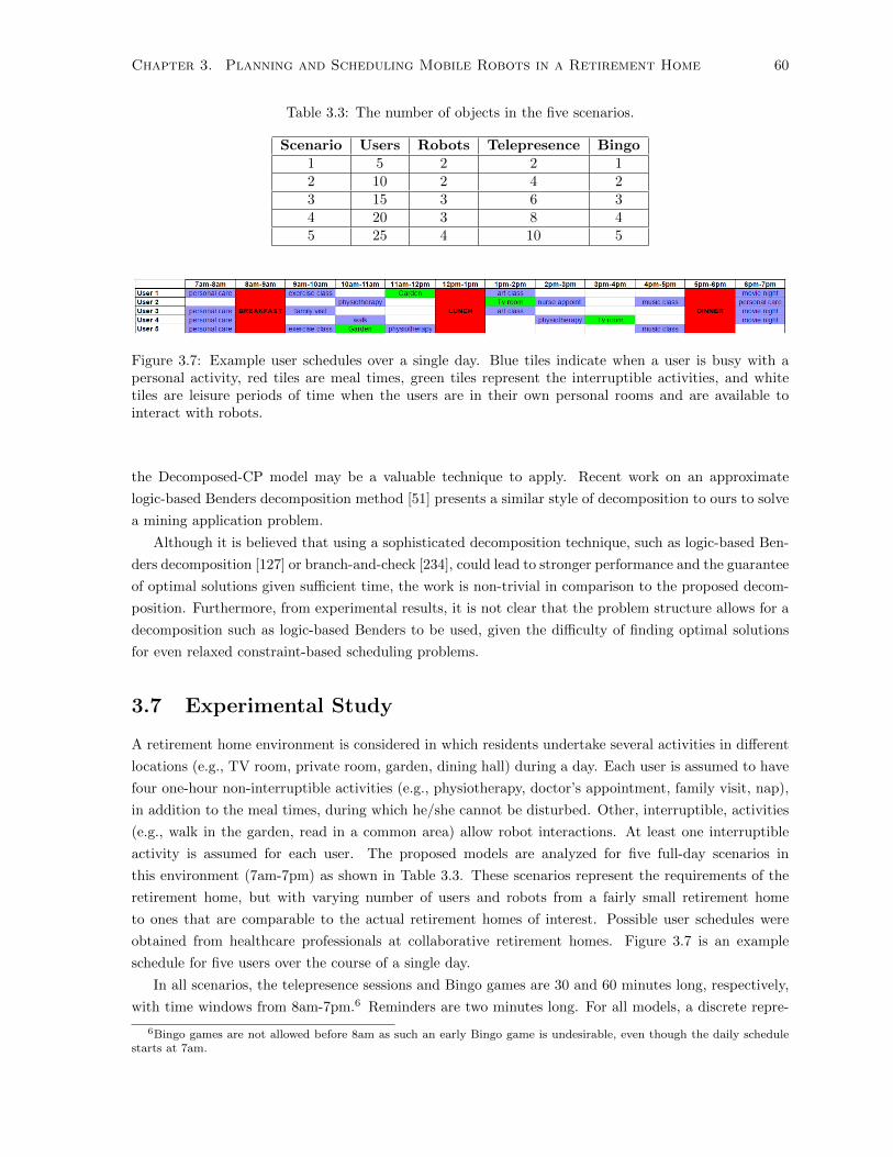
Chapter 3. Planning and Scheduling Mobile Robots in a Retirement Home 60
Table 3.3: The number of objects in the five scenarios.
Scenario Users Robots Telepresence Bingo1 5 2 2 12 10 2 4 23 15 3 6 34 20 3 8 45 25 4 10 5
Figure 3.7: Example user schedules over a single day. Blue tiles indicate when a user is busy with apersonal activity, red tiles are meal times, green tiles represent the interruptible activities, and whitetiles are leisure periods of time when the users are in their own personal rooms and are available tointeract with robots.
the Decomposed-CP model may be a valuable technique to apply. Recent work on an approximate
logic-based Benders decomposition method [51] presents a similar style of decomposition to ours to solve
a mining application problem.
Although it is believed that using a sophisticated decomposition technique, such as logic-based Ben-
ders decomposition [127] or branch-and-check [234], could lead to stronger performance and the guarantee
of optimal solutions given sufficient time, the work is non-trivial in comparison to the proposed decom-
position. Furthermore, from experimental results, it is not clear that the problem structure allows for a
decomposition such as logic-based Benders to be used, given the difficulty of finding optimal solutions
for even relaxed constraint-based scheduling problems.
3.7 Experimental Study
A retirement home environment is considered in which residents undertake several activities in different
locations (e.g., TV room, private room, garden, dining hall) during a day. Each user is assumed to have
four one-hour non-interruptible activities (e.g., physiotherapy, doctor’s appointment, family visit, nap),
in addition to the meal times, during which he/she cannot be disturbed. Other, interruptible, activities
(e.g., walk in the garden, read in a common area) allow robot interactions. At least one interruptible
activity is assumed for each user. The proposed models are analyzed for five full-day scenarios in
this environment (7am-7pm) as shown in Table 3.3. These scenarios represent the requirements of the
retirement home, but with varying number of users and robots from a fairly small retirement home
to ones that are comparable to the actual retirement homes of interest. Possible user schedules were
obtained from healthcare professionals at collaborative retirement homes. Figure 3.7 is an example
schedule for five users over the course of a single day.
In all scenarios, the telepresence sessions and Bingo games are 30 and 60 minutes long, respectively,
with time windows from 8am-7pm.6 Reminders are two minutes long. For all models, a discrete repre-
6Bingo games are not allowed before 8am as such an early Bingo game is undesirable, even though the daily schedulestarts at 7am.

Chapter 3. Planning and Scheduling Mobile Robots in a Retirement Home 61
Table 3.4: Performance of the proposed models on problem BRPOF. The “virtual best” results over allsix PDDL planning models for each scenario is presented. A (-) indicates that no solution was found.
Model Scenario Runtime (s) Participants Objective Valuefirst last first last first last
1 0.74 2,033.72 3 4 2,147.10 1,124.112 0.68 2,062.94 0 0 11,012.37 11,012.23
PDDL 3 57.16 1,960.02 0 0 16,518.65 16,518.63Planning 4 2.18 23.84 0 0 22,024.92 22,024.92
5 7.24 89.46 0 0 27,557.30 27,554.54
1 0.16 3,278.58 0 5 5540.00 481.552 3.24 3,464.43 0 8 11,024.00 2,954.48
MIP 3 277.64 595.80 0 0 16,518.91 16,518.914 1,285.76 1,285.76 0 0 22,064.25 22,064.255 - - - - - -
1 0.08 9.26 0 5 5,623.00 192.002 1.96 33.84 6 9 4,549.00 1,243.00
Global-CP 3 - - - - - -4 - - - - - -5 - - - - - -
1 0.05 0.23 5 5 486.00 192.002 0.08 67.49 6 10 5,039.00 847.00
Decomposed 3 0.36 37.87 4 15 12,296.00 1,213.50CP 4 0.41 2,567.80 10 20 12,107.00 1,430.50
5 0.37 3,382.83 4 25 23,494.50 1,929.00
sentation of time is used in increments of one minute. Each game has a minimum of three participants
and a maximum of ten participants. Every user is willing to attend at most one Bingo game during the
day (i.e., att min = 0, att max = 1). All robots have the following property values, estimated based
on the Tangy robot: bl min = 0, bl = bl max = 20, v = 20m/min, rr = 0.5, cr move = 0.04, and
cr telep = cr remind = cr Bingo = 0.1.
Each model is run on the five scenarios using a 64-bit Ubuntu Linux machine with 32 GB of memory.
The OPTIC planner [35] is used to solve the PDDL planning model. Preliminary experiments tested
five different planners: COLIN [64], LPG-td [102], OPTIC [35], POPF [63], and SGPlan [128]. Of the
five planners, only COLIN, OPTIC, and POPF were able to find feasible plans for the smallest scenario
tested. OPTIC was found to be the best performing solver of the five. The MIP and CP models are solved
using IBM ILOG Optimization Studio 12.6.2 with CPLEX and CP Optimizer solvers, respectively. A
one-hour timeout was used for each model in each scenario. The runtime, the number of users attending
a game, and the solution quality based on the objective function of problem BRPOF are compared as
a performance metric.
For a given problem modification, all solvers search an equivalent solution space and objective func-
tion. During the one-hour time limit, the first and last solution found using each of the models was
recorded. The only objective function that is not calculated based on the full objective is for problem
variation -RPOF, where the battery usage criteria is ignored. Thus, the objective function used in prob-
lem variation -RPOF removes the battery usage and only includes the user participation, Bingo games
played, and delivery time components. As such, the objective value for -RPOF will seem better than

Chapter 3. Planning and Scheduling Mobile Robots in a Retirement Home 62
it should be if the same schedule were to be applied to other problem variations as there will be an in-
crease in cost from battery usage (assuming that the schedule is also feasible when battery consumption
is considered).
Table 3.4 presents the results for the five scenarios using the different solvers on problem BRPOF. The
best results, based on the final objective value score, are provided over the six different PDDL planning
models for each of the five scenarios individually. That is, the PDDL results represent the virtual best
over all PDDL models. PDDL planning is able to find feasible plans for all scenarios, however, Bingo
games are only played in Scenario 1. The MIP solver finds good schedules for scenarios 1 and 2, but
poor schedules for scenarios 3 and 4, and no feasible schedule for scenario 5. CP Optimizer has problems
finding even feasible solutions for larger scenarios (3-5) when using the Global-CP model. However, for
the scenarios where solutions are found, Bingo games are played and the user participation is high. CP
Optimizer with the Decomposed-CP model is able to find high quality solutions for all scenarios and is
consistently the best performing method.7
In the rest of this section, the experiments for each methodology are presented. The performance
of these approaches are shown under various problem modifications and the different approaches are
discussed in more detail.
3.7.1 PDDL-based Planning
Table 3.5 presents the results of running the OPTIC planner on all six models on problem BRPOF.
Overall, good quality solutions, meaning high user participation in Bingo games, are only found for
the smallest scenario. All models that make use of the larger action that acts as an envelope over all
Bingo related activities are unable to find feasible solutions for Scenarios 2-5. Introducing the required
concurrency between the Bingo overall action and remind, setup Bingo, and play Bingo gives the planner
difficulty as the problem size increases. Thus, the envelope modeling strategy does not scale well.
Worse performance from set-all is seen when compared to single and min-add. The problem with
set-all is the large number of grounded play Bingo actions in the larger scenarios. Although min-add
also has many grounded actions, the total number of grounded play Bingo actions is significantly fewer
than for set-all. Only the single modeling strategy scales the number of grounded interaction actions
linearly with the number of users and Bingo games. The other alternatives require(NX
)grounded actions
for each play BingoX operator, where N is the total number of users. Thus, even for strategy min-add
with X = 3, scenarios with large N are intractable.
Table 3.6 illustrates the planning model performances on the BRPO- problem providing insights into
the behavior of the planner and showing the best performance obtained over all problem modifications.
The planning models generally behave as in Table 3.5, except for single-envelope. The larger scenarios are
still not solved, but high quality solutions are found for Scenarios 1-3. The change that allows for better
performance here is the removal of the clock-ticker process completely, since BRPO- is not concerned
with the delivery time in the objective function and the envelope modeling strategy handles separation
constraints by using the Bingo overall action. As expected, grounding many actions for min-add and
set-all is still very difficult for the larger scenarios, but under the single-envelope model, it is possible to
obtain solutions for up to the medium-sized scenarios.
Full results for all six PDDL models and seven problem modifications can be found in the Appendix
7Recall that due to the limitations of the timeline-based planner and scheduler as outlined in Section 3.4.1, the problemwas not fully modeled and therefore no solutions are obtained.

Chapter 3. Planning and Scheduling Mobile Robots in a Retirement Home 63
Table 3.5: Performance of PDDL planning on the BRPOF problem. A (-) indicates that no solutionwas found.
Problem Scenario Runtime (s) Participants Objective Valuefirst last first last first last
1 0.04 786.12 0 3 5,506.13 2,070.752 0.18 0.88 0 0 11,019.38 11,016.66
single-clock 3 0.84 9.38 0 0 16,530.31 16,525.734 2.18 23.84 0 0 22,044.46 22,043.115 7.24 89.46 0 0 27,557.30 27,554.54
1 0.06 2,950.88 0 3 5,506.13 2,066.512 0.68 2,062.94 0 0 11,012.37 11,012.23
min-add-clock 3 57.16 1,960.02 0 0 16,518.65 16,518.634 143.36 143.36 0 0 22,024.92 22,024.925 - - - - - -
1 0.74 2,033.72 3 4 2,147.10 1,124.112 - - - - - -
set-all-clock 3 - - - - - -4 - - - - - -5 - - - - - -
1 0.84 1,287.07 3 3 2,152.33 2,077.942 - - - - - -
single-envelope 3 - - - - - -4 - - - - - -5 - - - - - -
1 0.84 1,287.07 3 3 2,152.333 2,077.942 - - - - - -
min-add-envelope 3 - - - - - -4 - - - - - -5 - - - - - -
1 0.76 943.56 3 3 2,152.33 2,077.942 - - - - - -
set-all-envelope 3 - - - - - -4 - - - - - -5 - - - - - -
C in Tables C.1 - C.6. In general, OPTIC is observed to have a difficult time finding solutions with active
Bingo games. Removal of battery consideration and separation constraints helps the planner, but does
not lead to a significant improvement. At best, these problem modifications led to Bingo games being
played for Scenarios 1 and 2 rather than just Scenario 1. Interestingly, for most models, the planner
has a harder time when Bingo games are forced to be played and in fact, more often than not, fails to
find any solutions when Bingo games cannot be skipped, even though the same model is able to find a
solution with a Bingo game when the skip Bingo operator is included.
When Bingo games are restricted to have exactly four participants, the planner is unable to find a
solution for Scenario 1 with any Bingo games except for the single-envelope model. Lastly, the problem
B—F can help the performance as the solver is able to find plans with two games in Scenario 2 for the
single-clock model. However, the other models do not see any improvements.
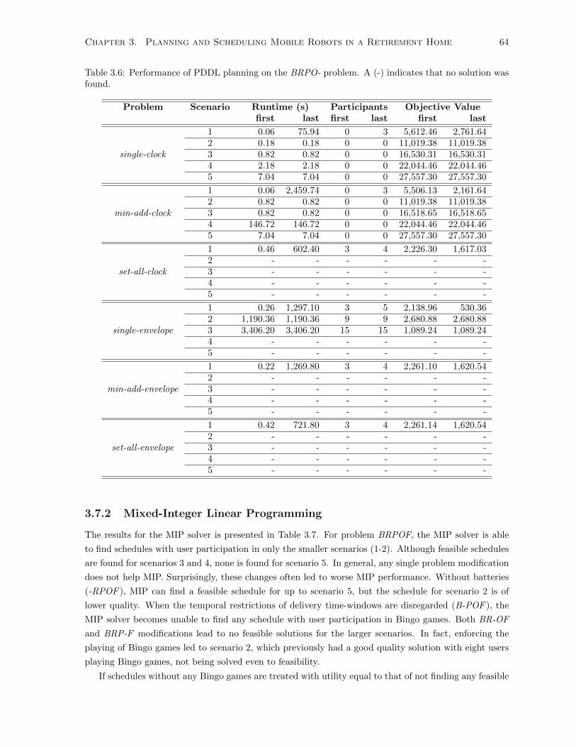
Chapter 3. Planning and Scheduling Mobile Robots in a Retirement Home 64
Table 3.6: Performance of PDDL planning on the BRPO- problem. A (-) indicates that no solution wasfound.
Problem Scenario Runtime (s) Participants Objective Valuefirst last first last first last
1 0.06 75.94 0 3 5,612.46 2,761.642 0.18 0.18 0 0 11,019.38 11,019.38
single-clock 3 0.82 0.82 0 0 16,530.31 16,530.314 2.18 2.18 0 0 22,044.46 22,044.465 7.04 7.04 0 0 27,557.30 27,557.30
1 0.06 2,459.74 0 3 5,506.13 2,161.642 0.82 0.82 0 0 11,019.38 11,019.38
min-add-clock 3 0.82 0.82 0 0 16,518.65 16,518.654 146.72 146.72 0 0 22,044.46 22,044.465 7.04 7.04 0 0 27,557.30 27,557.30
1 0.46 602.40 3 4 2,226.30 1,617.032 - - - - - -
set-all-clock 3 - - - - - -4 - - - - - -5 - - - - - -
1 0.26 1,297.10 3 5 2,138.96 530.362 1,190.36 1,190.36 9 9 2,680.88 2,680.88
single-envelope 3 3,406.20 3,406.20 15 15 1,089.24 1,089.244 - - - - - -5 - - - - - -
1 0.22 1,269.80 3 4 2,261.10 1,620.542 - - - - - -
min-add-envelope 3 - - - - - -4 - - - - - -5 - - - - - -
1 0.42 721.80 3 4 2,261.14 1,620.542 - - - - - -
set-all-envelope 3 - - - - - -4 - - - - - -5 - - - - - -
3.7.2 Mixed-Integer Linear Programming
The results for the MIP solver is presented in Table 3.7. For problem BRPOF, the MIP solver is able
to find schedules with user participation in only the smaller scenarios (1-2). Although feasible schedules
are found for scenarios 3 and 4, none is found for scenario 5. In general, any single problem modification
does not help MIP. Surprisingly, these changes often led to worse MIP performance. Without batteries
(-RPOF ), MIP can find a feasible schedule for up to scenario 5, but the schedule for scenario 2 is of
lower quality. When the temporal restrictions of delivery time-windows are disregarded (B-POF ), the
MIP solver becomes unable to find any schedule with user participation in Bingo games. Both BR-OF
and BRP-F modifications lead to no feasible solutions for the larger scenarios. In fact, enforcing the
playing of Bingo games led to scenario 2, which previously had a good quality solution with eight users
playing Bingo games, not being solved even to feasibility.
If schedules without any Bingo games are treated with utility equal to that of not finding any feasible

Chapter 3. Planning and Scheduling Mobile Robots in a Retirement Home 65
Table 3.7: Performance of MIP on all tested problem modifications. A (-) indicates that no solution wasfound.
Problem Scenario Runtime (s) Participants Objective Valuefirst last first last first last
1 0.16 3,278.58 0 5 5,540.00 481.552 3.24 3,464.43 0 8 11,024.00 2,954.48
BRPOF 3 277.64 595.80 0 0 16,518.91 16,518.914 1,285.76 1,285.76 0 0 22,064.25 22,064.255 - - - - - -
1 0.58 17.62 0 5 5,500.00 468.002 3.46 3,561 0 7 11,000.00 3,674.00
-RPOF 3 7.91 7.91 0 0 16,500.00 16,500.004 23.70 23.70 0 0 22,000.00 22,000.005 361.67 361.67 0 0 27,500.00 27,500.00
1 0.75 5.66 0 0 5,540.00 5,506.122 2.80 467.72 0 0 11,024.46 11,012.39
B-POF 3 40.35 2,178.44 0 0 16,537.00 16,518.734 30.10 30.10 0 0 22,055.32 22,055.325 - - - - - -
1 6.19 3,424.82 4 4 1,435.06 1,345.002 1,080.53 2,443.57 8 8 2,999.18 2,996.07
BR-OF 3 - - - - - -4 - - - - - -5 - - - - - -
1 0.72 531.75 3 5 2,389.00 481.552 - - - - - -
BRP-F 3 - - - - - -4 - - - - - -5 - - - - - -
1 0.76 4.18 0 5 5,562.00 583.242 3.14 3,291.65 0 7 11,035.04 3,709.41
BRPO- 3 41.49 41.49 0 0 16,537.00 16,537.004 - - - - - -5 - - - - - -
1 0.89 2.16 4 4 1,533.30 1,532.842 51.41 108.06 8 8 3,617.51 3,097.82
B—F 3 - - - - - -4 - - - - - -5 - - - - - -
schedule at all (given that a major motivation of using these mobile robots in a retirement home is to
foster social interaction), the modifications result in either worse performance (B-POF and BRP-F ) or
roughly equivalent performance (-RPOF, BR-OF, BRPO-, and B—F ).
3.7.3 Constraint Programming
In this section the experimental results of both the Global-CP and the Decomposed-CP models using
CP Optimizer are presented.

Chapter 3. Planning and Scheduling Mobile Robots in a Retirement Home 66
3.7.3.1 Global-CP
Table 3.8 presents the results from running the CP solver on the different problem modifications using
the Global-CP model. For problem BRPOF, CP is only able to find solutions for Scenarios 1 and 2.
With more than 10 users and 2 robots, CP cannot obtain feasible solutions within the one-hour time
limit. CP can only obtain solutions to bigger problems (Scenarios 3-5) when batteries (B), the reminder
time bounds (R), or the complex objective function (F ) are removed. Of those three properties, the
reminder time bounds (R) has a much smaller effect as B-POF can only solve up to Scenario 3. CP
performs well on -RPOF, BRPO-, and B—F. In all three of these problems, CP obtains solutions for all
five scenarios.
Problem BRPO- provides an interesting and unexpected result. Changing the objective function to
only consider user participation leads to CP finding solutions quickly (within fractions of a second) and
with maximum user participation. This result is against expectation as one of the main advantages of
CP is its strong inference methods, which we might expect would not be effected by the removal of the
complex objective function. More specifically, one would have expected potentially stronger performance
when altering the objective function in regards to optimizing schedules, but the fact that even finding
satisficing schedules became significantly easier was not expected.
Table 3.8 gives insights into the problem components that are difficult for the CP model. It is clear
that battery level considerations and complex objective functions lead to the majority of the issues when
trying to find even feasible solutions. When either of these are removed, CP does not have trouble
quickly obtaining solutions with everyone playing Bingo games.
3.7.3.2 Decomposed-CP
Table 3.9 provides the performance of the decomposition model for the different problem modifications.
The first solution presented is the first feasible schedule found by the first stage of the Decomposed-CP
model. Recall that the first stage is a sound model and so produces globally feasible solutions.
The decomposition is able to find schedules with the maximum number of possible participants for
every scenario and in general to do so very quickly. Note that for problem variations B—F and BR-OF,
the maximum number of participants is limited by the restriction on the number of users in a game,
which is less than the total number of users. These results were expected after observing the performance
of Global-CP, since, as mentioned earlier, the first stage of the decomposition is the Global-CP applied
to problem BRPO-.
Using the first stage results to restrict the second stage makes the problem tractable for all tested
scenarios. Once a partial schedule is found with decisions made regarding the presence of a Bingo game
and its players, the problem becomes significantly easier as many actions with cascading dependencies
are eliminated. There is a large reduction in the number of charging tasks (about 98%) and reminder
tasks (between 80% and 96%). As was seen with the Global-CP model, battery level considerations
make the problem hard and removal of just that aspect of the problem led to substantial performance
improvements.
3.7.4 Best Performance Results
Table 3.10 presents the best performance of each approach when considering all the sound problem mod-
ifications: BRPOF, BR-OF, BRP-F, and BRPO-. The quality of the solutions generated are compared

Chapter 3. Planning and Scheduling Mobile Robots in a Retirement Home 67
Table 3.8: Performance of Global-CP on all tested problem modifications. A (-) indicates that nosolution was found.
Problem Scenario Runtime (s) Participants Objective Valuefirst last first last first last
1 0.08 9.26 0 5 5,623.00 192.002 1.96 33.84 6 9 4,549.00 1,243.00
BRPOF 3 - - - - - -4 - - - - - -5 - - - - - -
1 0.08 0.15 5 5 223.00 178.002 0.11 48.73 10 10 807.00 276.00
-RPOF 3 0.46 337.67 14 15 2,352.00 359.004 0.91 3,040.75 20 20 2,006.00 450.005 1.66 2,870.58 24 25 4,646.00 550.00
1 0.08 41.75 5 5 1,745.00 192.002 0.36 256.49 8 10 4,885.00 346.00
B-POF 3 2,230.32 2,230.32 15 15 5,176.00 5,176.004 - - - - - -5 - - - - - -
1 0.11 2,297.28 4 4 1,447.00 1,129.502 0.49 925.55 8 8 2,817.00 2,179.50
BR-OF 3 - - - - - -4 - - - - - -5 - - - - - -
1 0.40 18.83 5 5 499.00 192.002 0.87 1,399.25 8 10 2,937.00 305.50
BRP-F 3 - - - - - -4 - - - - - -5 - - - - - -
1 0.05 0.05 5 5 486.00 486.002 0.08 24.22 6 10 5,039.00 847.00
BRPO- 3 0.36 37.87 4 15 12,296.00 2,013.504 0.41 1,076.5 10 20 12,107.00 2,522.005 0.37 103.33 4 25 23,494.50 3,033.50
1 0.27 28.88 4 4 1,387.50 1,129.502 0.18 2,022.39 8 8 4,144.00 2,262.00
B—F 3 25.83 3,590.05 12 12 5,366.50 3,428.004 1,162.26 1854.93 16 16 7,309.00 4,589.005 1,813.50 3501.50 20 20 9,473.50 5,960.50
using the objective function for the original problem. The problem that leads to the best final schedule
results for each method was chosen and these results compared. Furthermore, for the planning models,
since there are six different models, what is considered the best performing model based on the ability to
obtain better objective values (single-envelope) is chosen under the best performing problem modifica-
tion. For the planning solver and Global-CP, the best performance is found in problem BRPO-, whereas
MIP obtains the best solutions on problem BRPOF and Decomposed-CP works best with BRP-F.
The planning and CP-based methods are able to produce schedules for the robots in the system
sizes that are tested, but if the planning model that finds the most user participation in Bingo games

Chapter 3. Planning and Scheduling Mobile Robots in a Retirement Home 68
Table 3.9: Performance of the Decomposed-CP model on all tested problem modifications. The firstsolution that is recorded is based on the solution found from the first stage of the Decomposed-CPmodel.
Problem Scenario Runtime (s) Participants Objective Valuefirst last first last first last
1 0.05 0.23 5 5 486.00 192.002 0.08 67.49 6 10 5,039.00 847.00
BRPOF 3 0.36 37.87 4 15 12,296.00 1,213.504 0.41 2,567.80 10 20 12,107.00 1,430.505 0.37 3,382.83 4 25 23,494.50 1,929.00
1 0.26 0.29 5 5 473.00 178.002 0.01 0.09 0 10 11,000.00 364.00
-RPOF 3 0.04 170.31 0 15 16,500.00 678.004 0.06 1.06 0 20 22,000.00 783.005 0.08 12.64 0 25 27,500.00 723.00
1 0.27 0.49 5 5 1,397.00 192.002 0.06 36.16 6 10 4,471.00 642.50
B-POF 3 0.89 608.66 3 15 13,188.00 1,587.004 0.58 2,739.24 6 20 16,493.00 1,614.005 0.39 2,179.80 6 25 21,522.00 1,978.00
1 0.26 0.76 4 4 1,373.00 1,129.502 0.06 7.95 4 8 6,517.00 2,264.50
BR-OF 3 0.14 76.15 4 12 12,130.00 3,471.004 0.22 838.98 8 16 13,784.00 4,826.005 0.44 562.93 4 20 23,075.00 6,381.50
1 0.34 0.18 5 5 503.00 192.002 0.47 291.48 8 10 2,937.00 305.50
BRP-F 3 0.75 3,559.85 9 15 6,298.00 627.004 1.05 2,468.11 12 20 8,564.00 817.005 1.66 2,880.74 15 25 11,090.00 2,242.50
1 0.05 0.05 5 5 486.00 486.002 0.08 24.22 6 10 5,039.00 847.00
BRPO- 3 0.36 37.87 4 15 12,296.00 2,013.504 0.41 1,076.5 10 20 12,107.00 2,522.005 0.37 103.33 4 25 23,494.50 3,033.50
1 0.60 12.89 4 4 2,530.00 1,172.002 0.08 3,249.35 8 8 4,720.00 2,454.50
B—F 3 0.49 767.91 12 12 4,285.00 3,771.004 30.31 3,470.31 16 16 8,933.00 4,933.005 4.03 2,398.54 20 20 10,408.00 6,381.50
is chosen, the planner is unable to find feasible solutions for the larger scenarios. The planning solver
was found to perform worse than the two CP approaches even for scenarios where solutions are found.
MIP obtains solutions with user participation in Bingo games for scenarios 1 and 2, but does not handle
larger scenarios well. Only low quality feasible solutions with no Bingo games are found for scenarios
3 and 4, and not even a feasible schedule is found for scenario 5. Global-CP, with a simpler objective
function, is overall better than MIP and planning except in Scenario 3 where planning outperforms
Global-CP. By abstracting the objective and ignoring certain components that are considered of lesser

Chapter 3. Planning and Scheduling Mobile Robots in a Retirement Home 69
Table 3.10: Performance of the proposed models using the best modifications. A (-) indicates that nosolution was found.
Model Scenario Runtime (s) Participants Objective Valuefirst last first last first last
1 0.26 1,297.10 3 5 2,138.96 530.36Planning 2 1,190.36 1,190.36 9 9 2,680.88 2,680.88(BRPO-) 3 3,406.20 3,406.20 15 15 1,089.24 1,089.24
(single-envelope) 4 - - - - - -5 - - - - - -
1 0.16 3,278.58 0 5 5540.00 481.552 3.24 3,464.43 0 8 11,024.00 2,954.48
MIP 3 277.64 595.80 0 0 16,518.91 16,518.91(BRPOF) 4 1,285.76 1,285.76 0 0 22,064.25 22,064.25
5 - - - - - -
1 0.05 0.05 5 5 486.00 486.002 0.08 24.22 6 10 5,039.00 847.00
Global-CP 3 0.36 37.87 4 15 12,296.00 2,013.50(BRPO-) 4 0.41 1,076.5 10 20 12,107.00 2,522.00
5 0.37 103.33 4 25 23,494.50 3,033.50
1 0.34 0.18 5 5 503.00 192.002 0.47 291.48 8 10 2,937.00 305.50
Decomposed-CP 3 0.75 3,559.85 9 15 6,298.00 627.00(BRP-F) 4 1.05 2,468.11 12 20 8,564.00 817.00
5 1.66 2,880.74 15 25 11,090.00 2,242.50
importance, Global-CP becomes a much more attractive option. The Decomposed-CP model, which has
the Global-CP strengths on the BRPO- problem by design, is the superior choice as the components
ignored in the objective initially are re-introduced into the sub-problem.
3.8 Discussion
The overall robot project requires research and development on multiple fronts. This study considers
the issue of which technology to adopt for the planning and scheduling components of the system. Based
on the results that are obtained, CP is currently the more suitable technology.
While all four technologies can be further improved with intelligent modeling choices and search guid-
ance, the results presented demonstrate the baseline performance one achieves when following standard
modeling approaches for the different technologies along with current state-of-the-art solvers. From this
study, once can identify issues which indicate the research directions that need to be further explored in
order to adequately handle this application as well as those similar to it.
3.8.1 PDDL-Based Planning
As noted in the discussion of the limitations and issues with PDDL planning, representation of temporal
constraints is a challenge. While substantial use of the calendar in CP is made, enforcing temporal
consistency with the temporal representation in PDDL (e.g., TILs) is difficult and the current approaches
do not have an intuitive representation as compared to simple temporal networks and scheduling models

Chapter 3. Planning and Scheduling Mobile Robots in a Retirement Home 70
[70, 173]. In addition Cushing and Kambhampati [70] state that most temporal planners are incomplete
due to restrictions of action start times to a small set of time points called decision epochs. Nonetheless,
using decision epochs drastically improves computational performance and allows improved techniques
from classical planners to be directly used for temporal planners. It is clear from the results that the use
of the clock process to capture the temporal separation has significant negative impact on performance.
Thus, improvement on handling processes more efficiently is a fruitful direction.
The performance of and accessibility to model features in planners can be improved. One example is
the unavailability of the forall feature in conjunction with other features, greatly limiting the modeling
options. This issue is noted in the literature for most state-of-the-art planners [12]. Even with the features
that could be used, like optimization, the planner was found to generally not be able to significantly
improve solutions. Benton et al. [35] discuss the limitations of optimization in planners and propose the
OPTIC planner for optimization of continuous models. The experiments illustrate that planners still
have much to gain from additional efforts in this area. Most of the final solutions found using OPTIC
were similar in quality to the first solution found and those plans were of very poor quality. To address
problems similar to ours, planners must develop improved abilities to solve problems with temporal
reasoning and concurrency [70, 135], numeric values [65, 130], and optimization [35].
3.8.2 Timeline-Based Planning and Scheduling
EUROPA presents a step in the right direction in temporal representation as the NDDL and ANML
languages provide a more intuitive representation of temporal characteristics via timelines. However,
both modeling languages share the same problem of having minimal support from solvers capable of
handling the full set of language features. While both are strong candidates for use, the current barrier
for timeline-based planning and scheduling to be competitive with PDDL-based planning and constraint-
based scheduling is the state of current solvers. With additional efforts towards the development of
solvers, timeline-based approaches will be a useful technology for problems similar to ours.
3.8.3 Mixed-Integer Programming
Of the three technologies studied that had sufficient solver support to handle the proposed models, MIP
is found to have the poorest performance. This result is expected for such a scheduling problem as
MIP has been generally found to be worse than CP for scheduling problems [47, 146]. As discussed in
Section 3.5.2, the restriction to linear constraints greatly limits the flexibility and increases the size of the
model. In general, most constraints in the MIP model are non-binding constraints and lead to significant
degradation in performance of the MIP solvers. However, these constraints are necessary to ensure the
validity of the model. Many MIP solvers support lazy constraints in an attempt to remove these non-
binding constraints from consideration during search, but the effects of these non-binding constraints
cannot be completely removed. Improving either the search procedure around these constraints or re-
modeling the MIP model itself to reduce the impact of these constraints can greatly help tractability.
Remodeling of the problem can be particularly useful for MIP. More so than the other technologies
studied in this work, MIP has had the most attention on the impact of modeling [145, 146, 172]. A
deeper study of alternative modeling practices for multi-robot task scheduling problems where there
are large sets of decision variables representing the same task can help to improve MIP performance.
In addition, further examination of the polytope of the feasible region can assist with creating strong
Chapter 3. Planning and Scheduling Mobile Robots in a Retirement Home 71
redundant constraints to help guide search [41]. The linear relaxation for this problem is generally very
weak so the branch-and-cut approach of MIP solvers will not be provided with strong search heuristics.
Thus, a better understanding of the modeling decisions necessary to obtain tighter linear relaxations
or methods to handle poor relaxations is necessary if MIP is to be competitive against the alternative
solvers in this application problem.
3.8.4 Constraint-Based Scheduling
While the decomposition-based CP model delivered satisfactory performance on the test set, there is
still room for improvement. Unlike the planning representation, it is not currently possible to model
operators that may be instantiated multiple times. Laborie [148] notes this issue when comparing
the planning and scheduling literature. Beck and Fox [28] extend propagation algorithms to handle
alternative activities that do not necessarily have to be executed in a schedule. Laborie and Rogerie
[150] introduce a framework for reasoning about conditional time-interval variables that is used in this
chapter to address this issue. However, this approach is not scalable. A valuable direction for researchers
in constraint-based scheduling is the development of a method to model and solve problems with these
reoccurring tasks. By being able to dynamically add tasks during problem solving, the size of the
model can be substantially reduced [24]. Yet, significant progress towards being able to competently
handle reoccurring tasks for complex environments in CP has not been made. The closest work is the
CPT planner, which combines partial order causal link branching with CP to obtain a strong pruning
mechanism that dynamically introduces actions in the CP model [252]. However, this functionality came
at the cost of substantial customization of the underlying CP solver.
CP also lacks the expressivity of planning and timeline-based planning and scheduling. For example,
the move action of the robot is represented in the CP models as transition times between actions.
However, given that the distance traveled by a robot is dependent on the location of the previous and
next actions and that action locations can depend on the time at which they are executed (e.g., users
move around during the day), there is no straightforward or efficient manner to model robot movement.
This is accomplished by creating alternative tasks for each activity at each potential location of a user,
but this approach will not scale well and is only possible because the problem of interest does not include
a large number of possible user locations. For similar robot scheduling problems in a larger environment,
the representation for robot movement used here may result in much poorer performance.
Finally, it was interesting to see that the complex objective function was so difficult for the CP
solver. A deeper analysis and understanding of how CP behaves under particular models, objectives,
and constraints would be useful. The current state-of-the-art in CP optimization techniques is either
hybridization with linear programming [119, 120, 151] or cost-aware constraints [90, 221, 208], neither
of which apply to complex, arbitrary non-linear objective functions.
3.8.5 The Effect of Modeling
Although multiple models are investigated, it is impossible to exhaust the complete model space to es-
tablish the best possible model for each technology. It is clear that modeling decisions can greatly impact
solver performance, but the choice of formulation is non-trivial. This problem is further confounded as
the performance of a model can depend on the solver that is chosen, requiring a user to have a strong
understanding of a specific solver’s inner workings in order to create efficient models. These issues are

Chapter 3. Planning and Scheduling Mobile Robots in a Retirement Home 72
true for all technologies studied. Neither AI planning nor CP has developed solver-independent and
formal ways of comparing alternative models for the same problem in the way, for example, that the
study of polyhedral theory has for mixed-integer linear programming [41, 218]. Nonetheless, to make
progress on solving interesting problems, modeling decisions must be made and conclusions drawn from
experimental studies.
There is not much work that deeply explores the study and development of modeling approaches and
strategies in either PDDL planning or CP scheduling.8 The current approach to modeling in planning
and scheduling is based strongly around personal expertise and trial and error. Given the impact that
different models or model refinements can have on the performance of solvers, it is important that one
develops a strong model in order to be able to draw proper conclusions [210, 247]. It would be of
substantial value to users of these technologies to have studies that develop principles and practices
of modeling. There is a particular research area dedicated to the modeling techniques and principles
for planning and scheduling problems: Knowledge Engineering for Planning and Scheduling (KEPS), a
workshop that has been at the International Conference on Automated Planning and Scheduling since
2008. Yet, to the authors’ knowledge, a detailed body of work does not exist that explores the impact
of modeling in planning and scheduling.
3.8.6 AI Planning vs. Constraint Programming
Within the narrow context of the robot application, the results in Section 3.7.4 suggest that CP is the
more promising approach to the problem. However, it is not the purpose of this work, nor would it be
appropriate, to make general conclusions about the relative problem solving abilities of the technologies
that are investigated. At the most, given the very sparse application of CP technology to robot planning
and scheduling problems and the contrastingly larger application of AI planning (e.g., the series of
PlanRob workshops and robotics tracks at the International Conference on Automated Planning and
Scheduling), the results here suggest that CP is an interesting technology to investigate for this domain.
A more intriguing comparison arises from the question of the knowledge permitted in a model.
In domain-independent planning, the modeler seeks to represent the “physics” of a problem without
representing what has been generically termed “search control knowledge” [45, 123]. Although domain-
independent planning comprises of the mainstream of AI planning, domain-configurable planning, which
uses a domain-independent search engine with domain control knowledge, also exists in the literature.
For example, TLPlan [11] and TALPlan [147] make use of control rules to prune the search space while
hierarchical task network planners such as O-Plan [231] and SHOP2 [183] use domain-specific knowledge
for decomposing tasks into subtasks. The justification for the restriction of search control knowledge is
that human planners are able to solve problems without being given such domain-specific rules. If one is
truly seeking to develop an artificially intelligent planner, then supplying such rules defeats this purpose
as well as requiring extra effort by the modeler.
In contrast, the primary tools for modeling in CP are precisely the addition of search control knowl-
edge in the form of redundant constraints, dominance rules, and dual variables [223]. For example, from
a domain-independent planning perspective, the derivation of an upper bound on the number of recharg-
ing actions of a robot (see Section 3.2.3) so that one can even represent the problem is search control
knowledge. As noted above, the CP community also has the goal of declarative problem solving [94],
8Even though MIP has significantly more work exploring modeling approaches and strategies, it is still non-trivial togenerate good MIP models for all problems.

Chapter 3. Planning and Scheduling Mobile Robots in a Retirement Home 73
but has taken a different path, allowing modelers to add search control knowledge with the justification
being that through the study of such knowledge, as initially derived by modelers, we will eventually
be able to automate its derivation. Such automated modeling and model reformulation studies form
an active part of the CP research (see works by Frisch et al. [95], Nightingale and Rendl [185], and the
series of ModRef workshops at the International Conference on Principles and Practice of Constraint
Programming).
It is beyond the purposes here to go further into this contrast which has historically been a subject
of debate in the AI planning community [121, 122, 257]. However, returning to the application-driven
motivation, from the narrow perspective of solving application problems, the domain-independent AI
planning field would seem to be operating at a self-imposed disadvantage compared to CP by maintaining
domain independence. Of course, if the restriction helps to more quickly understand and achieve the
broader goals of truly intelligent agents, the disadvantage may be worthwhile.
3.8.7 Decomposition: Benefits and Insights
The verdict of CP being the most suitable technology is largely a result of the application of an ap-
propriate decomposition. Using any of the technologies by purely modeling the problem (BRPOF ) and
relying on the solvers is not always viable option; particularly when faced with complex application prob-
lems with characteristics uncommonly represented or handled by a solver. Each technology struggles
due to various problem components, but the introduction of a decomposition compensates for potential
weaknesses of the solver.
Decomposed-CP is an example where problematic components of the scheduling problem are iden-
tified and their negative effects are reduced through the use of a decomposition. By studying the CP
performance on the different modifications, it is possible to characterize where the solver runs into dif-
ficulty. The problem is then deconstructed to take advantage of CP’s strengths and handle a problem
more amenable to the solver. This work provides insights into the performance of CP and also how one
can construct schedules by only considering a subset of identified problematic aspects in turn to ensure
each stage of the decomposition is tractable.
Although the removal of weaknesses associated with a solver is emphasized for developing a successful
decomposition, it is important to note the necessary strengths that must exist for a solver as well.
The Decomposed-CP is able to perform well because the Global-CP is able to effectively handle the
decomposed problems. Applying the same decomposition for any of the other technologies would not
lead to the same effectiveness observed with CP because the decomposed problem is still intractable for
these other solvers.
3.8.8 Future Work
There are a number of avenues of subsequent work arising from this study.
Advanced Decomposition Models Various PDDL planning models, a MIP model, and two CP
models are considered. Decompositions are commonly found in the scheduling community but less
so in the planning literature. It would appear valuable to incorporate decomposition into the PDDL
planning models. However, from the empirical results, it is not apparent how one should decompose
the problem for planning. Using a similar decomposition as CP would not greatly improve performance

Chapter 3. Planning and Scheduling Mobile Robots in a Retirement Home 74
as the best performance over all models tested for PDDL planning was only able to find solutions with
user participation for up to Scenario 3. By using such a decomposition, only poor quality solutions will
be generated for Scenarios 4 and 5. Alternatively, one could explore a hybrid decomposition where the
master problem is solved by CP as in Decomposed-CP and the sub-problem with planning. A similar
decomposition with a MIP master problem and planning sub-problem has been successful in solving an
application problem related to mining operations [51]. The benefits of CP has been shown in this chapter,
but one could potentially see the benefits of planning if it is possible to use the set-all modeling strategy
without the explosion of grounded actions as user participation could be fixed in the sub-problem.
Disturbances Beyond this study, an extension is to look at a more complex system where external
robot- or user-related events cause disturbances that prevent a daily schedule from being completed
properly. For example, a robot-related disturbance can be a failure to arrive at a planned destination
due to obstacles blocking its path or unexpectedly low battery level. User-related disturbances exist
since a person may not be located where the robot believes him/her to be. Additionally, he/she may
decide not to participate in an HRI activity and so the scheduler must alter the schedule accordingly.
Disturbance consideration is essential for ensuring that robots can operate in a dynamic environment
and that users will have a positive experience with and confidence in the robots. In this current study,
disturbances could be handled naively by generating a new plan starting at the time of any disturbance,
using the models presented in this paper. However, a deeper study is required to fully understand and
apply the models developed here to the application problem where disturbances are a serious concern.
The hope is to build techniques to identify if and when the current schedule is no longer executable due
to disturbances. Once such disturbances are identified, schedule repair, and in extreme cases replanning
and rescheduling, must be done so that the robots can continue to operate in the environment. The
plan is to evaluate and extend work in the planning literature that looks at generating plans to handle
environments with exogenous events [96, 179, 181].
To repair, replan, and/or reschedule, the planner and CP technologies can be explored in addition
to other technologies. For example, Markov decision processes have been used by the planning commu-
nity [88, 214], but were not used in this paper. Due to the complexity of the environment, the state
representation (that must include temporal and numeric states) would lead to a very large state-space.
However, given pre-generated schedules, it may be interesting to see if there is potential to use Markov
decisions processes to replan when disruptions occur.
3.9 Conclusion
Ten models using four technologies are proposed for the multiple robot, retirement home environment:
six PDDL-based planning models, a timeline-based planning and scheduling model, a mixed-integer
programing model, and two constraint programming models. The many properties of the problem
together create a complex problem to solve. Not only must the robots manage their battery power, but
they must also choose sequences of tasks such that an efficient path is followed. In addition, tasks have
time constraints and users have their own personal schedules. Based on numerical experiments, CP, in
particular a decomposition model using CP, is found to be the most suitable technology.
CP is better equipped than PDDL planning for handling optimization, but can struggle to find
feasible schedules for larger problems. Although CP performs favorably when considering optimization,

Chapter 3. Planning and Scheduling Mobile Robots in a Retirement Home 75
it is interesting to note that the best approach is to only consider a simple objective function. Although
the large number of optional tasks used in the CP model is also is a culprit for the poor performance,
it is suspected that for similar problems with complex objective functions, it is easier and likely just as
effective to decompose a CP model to handle the objective function in stages rather than to remove or
reduce the optional activities. Of course, it may be necessary to introduce both strategies to adequately
deal with even more difficult problems.
The study of the various PDDL-based planning models suggests the importance of understanding
modeling decisions. The different methods to represent interaction within Bingo games show that one
must be conscious of the inclusion of required concurrency and the number of grounded actions generated
by a particular model. Decisions that introduce a trade-off between these aspects can be the difference
between a planning model that easily finds feasible solutions, but with poor quality, and a model that
does not find feasible solutions for larger problems, but has improved quality for smaller problems.
Due to the complex reasoning that must be applied to handle all the aspects of the problem, no
solution technique is the perfect choice. This work illustrates some of the limitations of the current
techniques in planning and scheduling to deal with the problem of interest as well as the difficulties
in making comparisons between these technologies. All aspects of this problem have been studied in
the two fields of research, but together, these problem characteristics prove difficult for the available
solvers. This problem provides an interesting application that tests the existing planning and scheduling
technology and we hope that this work might spur research on the challenges identified. Ideally, advances
in planning and scheduling research will lead to solvers that are better equipped to solve problems similar
to this robot scheduling problem.

Chapter 4
Resource-Aware Scheduling for
Heterogeneous Data Centers9
In the previous chapter, a two-stage decomposition is developed with both components solved using
constraint programming (CP). The potential for such a decomposition to compensate for the deficiencies
of a solver is shown. In this chapter, a decomposition is presented which combines queueing theory
and combinatorial optimization. These two areas focus on different abstractions of a system (system
dynamics or combinatorics) and have developed tools to deal with those abstractions. However, in
systems where both the dynamics and the combinatorics are important aspects that affect decision
making, it is necessary for a scheduler to adequately represent both. Neither queueing theory nor
combinatorial optimization techniques alone is sufficient. Through a hybrid decomposition of these
techniques, both aspects of the system are represented and the scheduler performance is improved. In
contrast to the previous chapter where CP is capable of properly modeling all system aspects, but
struggles to solve the resulting system, the work in this chapter shows the benefits of using different
techniques at various stages to make use of the most appropriate tools.
4.1 Introduction
The cloud computing paradigm of providing hardware and software remotely to end users has become
very popular with applications such as e-mail, Google documents, iCloud, and dropbox. Large scale
data centers are used to provide these services to help improve resource utilization for users which can
share resources. By distributing resources, it is possible to serve a much larger group of users than
if each user had their own dedicated hardware as most, if not all, users do not constantly require the
resources. As such, a data center with enough resources to simultaneously cover all requests during peak
demand periods can provide sufficient computing resources to all users as though they each had their
own hardware.
Although the benefits of data centers are clear when sufficient resources are available, their appeal
can be challenged when one considers the possibility that the available hardware may not be sufficient
to handle peak demand. Under heavy loads, performance of the system can suffer as resource contention
9The work in this chapter is based on work published at the Multidisciplinary International Scheduling Conference:Theory & Applications [239], which was extended and is currently under review for the Journal of Scheduling.
76

Chapter 4. Resource-Aware Scheduling for Heterogeneous Data Centers 77
grows and user requests cannot be immediately processed, but must wait for machines to become avail-
able. Therefore, it is important to provide scheduling support so that efficient routing of jobs to machines
can be made to improve response times to end users. The problem of scheduling jobs onto machines
such that the multiple resources available on a machine (e.g., processing cores and memory) can handle
the assigned workload in a timely manner is studied.
A decomposition algorithm is developed to schedule jobs on a set of heterogeneous machines to
minimize mean job response time, the time from when a job enters the system until it starts processing
on a machine. The algorithm consists of three stages: 1) a queueing model is applied to an abstracted
representation of the problem based on pooled resources and jobs, 2) a combinatorial optimization
problem is solved which generates possible mixes of jobs that can be processed on machines, which is
then used within the framework of the queueing model to refine the solution of the first stage, and 3) a
dispatch policy is used online to try and realize the assignment from the second stage. The decomposition
is evaluated using an event-based simulation based on both job traces from one of Google’s compute
clusters [175] and carefully generated instances that test behavior as relevant independent variables are
manipulated. The proposed algorithm substantially outperforms a natural greedy policy that attempts
to minimize the response time of each arrival and the Tetris scheduler [109], a dispatching policy based
on heuristics for the multi-dimensional bin packing problem.
The proposed decomposition benefits from its ability to reason about both the long-term stochastic
behavior of the system and its short-term combinatorial aspects through use of queueing theory and
combinatorial scheduling models.
The rest of the chapter is organized into a definition of the data center scheduling problem in Section
4.2, a literature review in Section 4.3, a presentation of the proposed algorithm in Section 4.4, exper-
imental results in Section 4.5, and a discussion including future directions in Section 4.6. Section 4.7
concludes this chapter.
The following are the main contributions of this chapter:
• A hybrid queueing theoretic and combinatorial optimization scheduling algorithm is proposed for
a data center. By decomposing the problem, the algorithm is able to consider both the system
dynamics and complex combinatorics, providing a richer representation of the system than would
be commonly found in pure queueing theory or combinatorial scheduling approaches.
• The allocation linear programming (LP) model [8] used for distributed computing [6] is extended
to a data center that has machines with multi-capacity resources. A system with multi-capacity
resources can have idle resources while jobs are waiting in queue because the remaining available
resources of a machine is insufficient to handle the demand of the jobs. Thus, the proposed model
is more complex than the original allocation LP model as it accounts for these idle resources in its
representation of the behavior of the system.
• An empirical study of the scheduling algorithm is performed on both real workload trace data and
randomly generated data that shows that the decomposition performs orders of magnitude better
than existing techniques.

Chapter 4. Resource-Aware Scheduling for Heterogeneous Data Centers 78
1 2 3 4 5 6 7 8 9
1
2
3
4
Time
Pro
cess
ing
Co
res
Use
d
4 Processing Cores
1
23
4
5
6
10
(a) Processing cores
3
1
2
1 2 3 4 5 6 7 8 9
4
5
6
7
8
Time
Mem
ory
Use
d
8 GBs of Memory
1
2 3
4
5
6
10
(b) Memory
Figure 4.1: Resource consumption profiles
4.2 Problem Definition
The data center of interest is comprised of on the order of tens of thousands of independent servers
(also referred to as machines). These machines are not all identical; the machine population is divided
into different configurations denoted by the set M . Machines belonging to the same configuration are
identical in all aspects.
A machine configuration is classified based on its resources. For example, machine resources may
include the number of processing cores and the amount of memory, disk-space, and bandwidth. For this
study, the system is generalized to have a set of resources, R, which are limiting resources of the data
center. A machine of configuration j ∈M has cjl of resource l ∈ R, which defines the machine’s resource
profile. For a given machine configuration j there are nj identical machines.
Jobs arrive to the data center dynamically over time with the intervals between arrivals being in-
dependent and identically distributed (i.i.d.). Each job belongs to one of a set of K classes where the
probability of an arrival being of class k ∈ K is αk. We denote the expected amount of resource of type
l required by a job of class k as rkl. The resources required by a job define its resource profile, which
can be different from the resource profile of the job class as the latter is an estimate of a job’s actual
profile. The processing times for jobs in class k on a machine of configuration j are assumed to be i.i.d.
with mean 1µjk
. The associated processing rate is thus µjk.
Each job is processed on a single machine. However, a machine can process many jobs at once, as
long as the total resource usage of all concurrent jobs does not exceed the capacity of the machine.
Figures 4.1 depict an example schedule of six jobs on a machine with two limiting resources: processing
cores and memory. Here, the x-axis represents time and the y-axis the amount of resource. The machine
has four processing cores and eight GBs of memory. Note that the start and end times of each job are
the same in both figures, representing the job concurrently consuming resources from both cores and
memory during its processing time.
Any job that requires more resources than currently available on a machine must wait until sufficient
resources become available. A buffer of infinite capacity is assumed, where jobs can queue until they

Chapter 4. Resource-Aware Scheduling for Heterogeneous Data Centers 79
Not Yet Arrived
Awaiting Dispatch
Running
Waiting
ExitSubmit
Execute
Queue
Execute
Finish
Figure 4.2: Stages of job lifetime.
begin processing.
Figure 4.2 illustrates the states a job can go through in its lifetime. Each job begins outside the
system and joins the data center once submitted. At this point, the job can either be scheduled onto
a machine if there are sufficient resources or it can enter the queue and await execution. After being
processed, the job exits the data center.
A key challenge in the allocation of jobs to machines is that the resource usage is unlikely to exactly
match the resource capacity. As a consequence, small amounts of each resource are unused. This
phenomenon is called resource fragmentation in the literature [109], because while there may be enough
resources to serve another job, they are spread across different machines. For example, if a configuration
has 30 machines with eight cores available on each machine and each job requires exactly three cores,
the pooled machine can process 80 jobs in parallel on its 240 processors. In reality, of course, only
two jobs can be placed on each machine and so only 60 jobs can be processed in parallel. The effect
may be further amplified when multiple resources exist, as fragmentation could occur for each resource.
Thus, producing high quality schedules is a difficult task when faced with resource fragmentation under
dynamic job arrivals.
The problem addressed requires the assignment of dynamically arriving jobs to machines. Each job
has a resource requirement profile that is known once the job has arrived to the system. Machines in
the data center each belong to one machine configuration and each configuration has many identical
machines with the same resource capacities. The performance metric of interest is the minimization of
the system’s average job response time.
4.2.1 A Simple Example of the Data Center System
Assume that there are 10,000 machines, each belonging to one of two machine configurations. The
relevant parameters of the two machine configurations are presented in Table 4.1.
Jobs belong to one of three job classes as shown in Table 4.2. Jobs will arrive at some rate λ and
belong to one of the three job classes with equal probability. As the jobs arrive, they must be assigned

Chapter 4. Resource-Aware Scheduling for Heterogeneous Data Centers 80
Table 4.1: Example Machine Configurations.
Number of Number of Amount ofMachines (nj) Cores (cj1) Memory (cj2)
Configuration 1 5,000 4 8Configuration 2 5,000 4 16
Table 4.2: Example Job Classes.
Proportion Proc. Rate Proc. Rate Exp. Core Exp. Mem.(αk) Mach. 1 (µ1k) Mach. 2 (µ2k) Req. (rk1) Req. (rk2)
Class 1 13 1 2 1 6
Class 2 13 1 2 1 2
Class 3 13 2 4 2 4
and scheduled onto one of the 10,000 machines such that the total resource requirements of the jobs do
not exceed the capacity of the machine, cjl. Note however that the values in Table 4.2 are based on
expectations. Thus, jobs entering the system may differ and a job from class 1 may arrive and require
three units of time on a machine from configuration 1, one processing core, and four GBs of memory.
4.3 Related Work
Scheduling in data centers has received significant attention in the past decade. Mann [170] presents
a large variety of problem contexts and system characteristics, demonstrating that the literature has
focused on different aspects of the problem. Unfortunately, as Mann points out, the approaches are
mostly incomparable due to differences in the problem models. For example, some works consider cost
saving through decreased energy consumption from lowering thermal levels [229, 255], powering down
machines [38, 99], or geographical load balancing [155, 160]. These works typically attempt to minimize
costs or energy consumption while maintaining some guarantees on response time and throughput. Other
works are concerned with balancing energy costs, service level agreement performance, and reliability
[111, 112, 217].
The literature on schedulers for distributed computing clusters has focused heavily on fairness and
locality [129, 191, 258]. Optimizing these performance metrics leads to equal access to resources for
different users and the improvement of performance by assigning tasks close to the location of stored
data to reduce data transfer traffic. Locality of data has been found to be crucial for performance in
systems such as MapReduce, Hadoop, and Dryad when bandwidth capacity is limited [258]. This work
does not consider data transfer or equal access for different users as the problem considered focuses
on the heterogeneity of machines with regards to resource capacity. Such characteristics are already a
considerable challenge. It is left as future work to incorporate locality and fairness into the model.
Most research considers heterogeneity in the form of machine-dependent processing time and not
resource usage and capacity [6, 141, 206]. Without a model of resource usage, fragmentation cannot be
reasoned about, but efficient allocation of jobs to resources can still be an important decision. Kim et al.
[141] study the dynamic mapping of jobs to machines with varying priorities and soft deadlines. They
identify two scheduling heuristics as the best performers: Max-Max and Slack Sufferage. In the former,

Chapter 4. Resource-Aware Scheduling for Heterogeneous Data Centers 81
a job assignment is made by greedily choosing the mapping that has the best fitness value based on the
priority level of a job, its deadline, and the job processing time. Slack Sufferage chooses job mappings
based on which jobs suffer most if not scheduled onto their “best” machines. These two heuristics are
found to be comparable in performance to each other and outperformed all other heuristics tested.
Al-Azzoni and Down [6] also consider machine-dependent processing times and schedule jobs to
machines using a linear program (LP) to efficiently pair job classes to machines based on expected
processing times. The solution of the LP maximizes the system capacity and guides the scheduling rules
to reduce the long-run average number of jobs in the system. Further, they show that their heuristic
policy is guaranteed to be stable if the system can be stabilized. The model developed in this chapter
extends the LP due to Al-Azzoni and Down and applies it in the first two stages of the scheduler.
Another study that considers processing time as a source of resource heterogeneity extends the same
LP model as Al-Azzoni and Down to a Hadoop framework [206]. The authors compare their work
to the default scheduler used in Hadoop and the Fair-Sharing algorithm and demonstrate that their
algorithm greatly reduces the mean response time while maintaining competitive levels of fairness with
Fair-Sharing. These studies illustrate the importance of scheduling with processing time heterogeneity
in mind as they show the performance improvements using their models. While the focus of this work
is resource capacity heterogeneity, strong performance is demonstrated in experiments that also include
processing time heterogeneity (see Section 4.5.3.3).
Some work that studies resource usage and capacity as the source of heterogeneity makes use of a
limited set of virtual machines with pre-defined resource requirements to simplify the issue of resource
fragmentation. Maguluri et al. [168] examine a cloud computing cluster where virtual machines are
to be scheduled onto servers. There are three different types of virtual machines: Standard, High-
Memory, and High-CPU, each with fixed resource requirements. Based on these requirements and the
capacities of the servers, the authors determine all possible combinations of virtual machines that can
concurrently be placed onto each server. A preemptive algorithm is presented that considers the pre-
defined virtual machine combinations on servers and is shown to be throughput-optimal. Maguluri et
al. later extended their work to a queue-length optimal algorithm for the same problem in the heavy
traffic regime [167]. They propose a routing algorithm that assigns jobs to servers with the shortest
queue (similar to the Greedy algorithm presented in Section 4.3.1) and a mix of virtual machines to
assign to a server based on the same reasoning proposed for their throughput optimal algorithm. Since
the virtual machines have predetermined resource requirements, it is known exactly how virtual machine
types fit on a server without having to reason online about each assignment individually. Therefore it
is possible to obtain performance guarantees for the scheduling policies as one can accurately account
for the resource utilization of the virtual machines. However, the performance guarantees are only with
respect to virtual machines which represent upper bounds on the true resource usage. Resource idling
occurs when a job does not utilize all the resource in its virtual machine.
Ghodsi et al. [105] examine a system where fragmentation does occur, but they do not try to optimize
job allocation to improve response time or resource utilization. Their focus is solely on fairness of resource
allocation through the use of a greedy algorithm called Dominant Resource Fairness (DRF). Here, users
submit jobs and the scheduler aims to provide a fair share of resources to each of the users when
scheduling the jobs. They define the dominant resource of a user as the one for which the user has the
highest requirement normalized by the maximum resource capacity over all machines. For example, if a
user requests two cores and two GB of memory and the maximum number of cores and memory on any

Chapter 4. Resource-Aware Scheduling for Heterogeneous Data Centers 82
machine is four cores and eight GB, the normalized values would be 0.5 cores and 0.25 memory. The
dominant resource for the user would thus be cores. Each user is then given a share of the resources
with the goal that the proportion of dominant resources for each user is fair following Jain’s Fairness
Index [133]. This approach compares resources of different types as the consideration is based on a user’s
dominant resource.
The work closest to ours is the Tetris scheduler [109] which considers resource fragmentation, re-
sponse time and fairness as performance metrics. The proposed scheduler uses a linear combination of
two scoring functions: best fit and least remaining work first. The first score favors large jobs, while
the second favors small jobs. The authors compare their scheduler against DRF and demonstrate that
focusing on fairness alone can lead to poor performance, while efficient resource allocation can be im-
portant. A direct comparison of the scheduling algorithm to the Tetris Scheduler is made in Section 4.5
as it is the most suitable model with similar problem characteristics and performance metrics.
4.3.1 Algorithms for Comparison: A Greedy Dispatch Policy and the Tetris
Scheduler
Two schedulers are considered as benchmarks for the proposed model: a Greedy policy and the Tetris
scheduler. The Greedy dispatch policy provides a natural heuristic, which aims to quickly process jobs
by attempting to schedule them immediately if an available machine is found. The dispatching is done in
a first-fit manner where the machines are ordered in some arbitrary ordering (in this case, all machines
of the same configuration are clustered). In the case where no machines are available for immediate
processing, the job enters a queue. Here, each machine is assumed to have a queue of infinite length, and
the job is dispatched to the machine with the shortest queue of waiting jobs with ties favoring machines
based on the arbitrary ordering. If a queue forms, jobs are processed in first-come, first-serve order.
The Tetris scheduler [109] aims to improve packing efficiency and reduce average completion time
through use of a linear combination of two metrics. The packing efficiency metric is calculated by taking
the dot product of the resource profiles of a job and the resource availabilities on machines. If one
denotes r as a vector representing the resource profile of a job and C as the resource profile for the
remaining resources on a machine, the packing efficiency score can be defined as ω = r · C. A higher
score represents a better fit of a job on a machine. The second metric, the amount of work, is calculated
as the total resource requirements multiplied by the job duration. That is, given the processing time of
a job p, the work score is γ = pr · 1, where 1 is a vector of ones. The Tetris scheduler prioritizes jobs
with less work in order to reduce overall completion times of jobs. Given a weight, a ∈ [0, 1], the score
is calculated as a · ω − (1− a)γ.
The Tetris scheduler addresses resource fragmentation through the use of the packing efficiency score.
By placing jobs on machines with higher packing scores, the scheduler aims to match machines with
resource profiles that are similar to the job resource profiles. Tetris benefits from being able to make
packing decisions online. However, Tetris makes decisions myopically, without the foresight that new
jobs will be arriving.

Chapter 4. Resource-Aware Scheduling for Heterogeneous Data Centers 83
Figure 4.3: LoTES Algorithm.
4.4 LoTES Model
Long Term Evaluation Scheduling (LoTES) is proposed, a three-stage queueing-theoretic and optimiza-
tion hybrid approach. Figure 4.3 illustrates the overall scheduling algorithm. The first two stages are
performed offline and are used to guide the dispatching algorithm of the third stage. The dispatching
algorithm is responsible for assigning jobs to machines and is performed online. In the first stage, a
technique from the queueing theory literature, an allocation LP to represent the queueing system as
a fluid model where incoming jobs are considered as a continuous flow [8], is used. The LP finds an
efficient pairing of machine configurations to job classes, which are then used to restrict the pairings
that are considered in the second stage where a machine assignment LP model is used to assign specific
machines to serve job classes. In the final stage, jobs are dispatched to machines dynamically as they
arrive to the system with the goal of mimicking the assignments from the second stage.
4.4.1 Stage 1: Allocation of Machine Configurations
Andradottir et al.’s [8] allocation LP was created for a similar problem but with a single unary resource
per machine. The allocation LP finds the maximum arrival rate for a given queueing network such that
stability is maintained. Stability is a formal property of queueing systems [71] that can informally be
understood as implying that the expected queue lengths in the system remain bounded over time. It is
important to ensure that a system is stable, otherwise performance quickly deteriorates. The allocation
LP from the literature is modified to accommodate |R| resources for use in the decomposition.
Two abstractions of the system are made in the allocation LP: the aggregation of machines and jobs
and the fluid representation of jobs. The number of machines is reduced by combining each machine’s
resources to create a single super-machine for each configuration. Thus, there are exactly |M | pooled
machines (one for each configuration j) with capacity cjl × nj for resource l. The allocation LP ignores
resource fragmentation, treating the amount of incoming work of all jobs (a product of the processing time
and resource requirements) as a continuous fluid to be allocated to these super-machines to maximize the
amount of work that can be sustained. Thus, the allocation LP is a relaxation of the actual system where
jobs are discrete and machines do not share resources in an aggregated manner. These two relaxations
together allow the allocation LP to divide a job across multiple machines.
As an example assume jobs are processed at a rate of one job per minute on a machine and there
exist two machines. There is only a single resource with the machines each having a capacity of five

Chapter 4. Resource-Aware Scheduling for Heterogeneous Data Centers 84
and jobs requiring three units of the resource. In practice, only a single job can be processed on each
machine, so the maximum rate that this system can handle is two jobs per minute. If more than two
jobs arrive each minute, the system acquires a queue that continues to grow. The relaxation treats the
machines as a super-machine that has a capacity of 10, and furthermore, jobs are divisible such that a
machine can process a job while it has fewer resources than required. Then it is possible to fit 103 jobs
on the super-machine at any time and so the relaxed system can handle 103 job arrivals per minute.
The extended allocation LP is:
max λ (4.1)
s.t.∑j∈M
δjklcjlnjµjk ≥ λαkrkl k ∈ K, l ∈ R (4.2)
δjklcjlrkl
=δjk1cj1rk1
j ∈M,k ∈ K, l ∈ R (4.3)
∑k∈K
δjkl ≤ 1 j ∈M, l ∈ R (4.4)
δjkl ≥ 0 j ∈M,k ∈ K, l ∈ R (4.5)
The decision variable, λ, denotes the arrival rate of jobs to the system and the objective is to maximize
that rate, while maintaining stability. The LP determines δjkl, the fractional amount of resource l that
super-machine j devotes to job class k. Constraint (4.2) guarantees that sufficient resources are allocated
for the expected requirements of each class. Constraint (4.3) ensures that the resource profiles of the
job classes are properly enforced. For example, if the amount of memory required is twice the number
of cores required, the amount of memory assigned to the job class from a single machine configuration
must also be twice the core assignment. The allocation LP does not assign more resources than available
due to constraint (4.4). Finally, constraint (4.5) ensures the non-negativity of assignments.
Solving the allocation LP provides δ∗jkl values which are used in the second stage of LoTES to restrict
its search for efficient allocations of jobs to machines.
4.4.1.1 Example Allocation LP Solution
Solving the allocation LP for the example data center as presented in Section 4.2.1 leads to an arrival
rate, λ = 60, 000. To achieve this arrival rate, all the resources of Machine Configuration 1 are allocated
to jobs of Class 3. The cores of Machine Configuration 2 are divided evenly between Job Class 1 and 2,
but the memory is divided such that 75% is allocated to Job Class 1 and 25% is allocated to Job Class
2. Table 4.4 illustrates the total amount of resources that have been allocated to each job class from
each machine configuration and Table 4.3 shows the δjkl values.

Chapter 4. Resource-Aware Scheduling for Heterogeneous Data Centers 85
Table 4.3: Example resource allocation (δjklcjlrkl).
Mach. Conf. 1 Mach. Conf. 2Job Class Cores Memory Cores Memory
1 0 0 10,000 60,0002 0 0 10,000 20,0003 20,000 40,000 0 0
Table 4.4: Example resource allocation (δjkl).
Mach. Conf. 1 Mach. Conf. 2Job Class Cores Memory Cores Memory
1 0 0 0.5 0.752 0 0 0.5 0.253 1 1 0 0
4.4.1.2 Rationale for the Fluid Model
The first stage of the algorithm provides efficient matchings between job classes and machine configu-
rations for the latter two stages. Although the problem solved for this stage is a relaxation, it captures
the long-term behavior of the system.
It is hypothesized that reasoning about both the long-term stochastic behavior of the system and its
short-term combinatorial aspects is critical for strong performance. Since obtaining optimal solutions
to a model that can accurately represent both system dynamics and combinatorics is beyond existing
optimization techniques, a relaxation that focuses on the long-term performance is solved and the solution
to the relaxed problem is used to guide reasoning on the combinatorial components.
The allocation LP builds upon the strong analytical results from the queueing theory literature that
are able to deduce tight upper bounds on the achievable capacity and prescribe dispatching rules to
achieve the calculated bounds with an arbitrarily small approximation [6, 8]. What distinguishes this
allocation LP from that of previous work is the inclusion of multiple resources with capacity. This
addition leads to fragmentation, which results in the loss of the bound guarantee and in the need for
combinatorial reasoning. However, even without tight bounds on the capacity of a network, by taking into
account the allocation LP results, the later stages of LoTES incorporate information about the long-term
behavior of the system. Typically, such information is unavailable to combinatorial algorithms [233].
4.4.2 Stage 2: Machine Assignment
In the second stage of the algorithm, the δ∗jkl values from the allocation LP are used to guide the choice of
which job classes should be assigned to each machine. Here, fragmentation is considered and so each job
class and each machine are treated discretely, building specific configurations of jobs (which are called
“bins”) that result in tightly packed machines and then deciding which bin each machine emulates. As
this stage is also offline, the expected resource requirements for each job class are used.
In more detail, recall that the δ∗jkl values from the allocation LP provide a fractional mapping of the
resource capacity of each machine configuration to each job class. Based on the δ∗jkl values that are non-
zero, the expected resource requests of jobs and the capacities of the machines, the machine assignment
algorithm first creates job bins. A bin is any multi-set of job classes that does not exceed the capacity

Chapter 4. Resource-Aware Scheduling for Heterogeneous Data Centers 86
Figure 4.4: Feasible bin configurations.
of the machine (in expectation). A non-dominated bin is one that is not a subset of any other bin: if
any additional job is added to it, one of the machine resource constraints will be violated. Figure 4.4
presents the feasible region for an example machine. Assume that the machine has one resource (cores)
with capacity seven. There are two job classes, job class 1 requires two cores and job class 2 requires
three cores. The integer solutions represent the feasible bins. All non-dominated bins exist along the
boundary of the polytope since any solution in the polytope not at the boundary has a point above or
to the right that is feasible.
All non-dominated bins are exhaustively enumerated. The machine assignment model then decides
how many machines should emulate each non-dominated bin. Since the machines in each configuration
are identical, these numbers can then be trivially used to assign a bin to each machine. Thus, each
machine is mapped to a single bin, but multiple machines may emulate the same bin.
Algorithm 1 below generates all non-dominated bins. Define Kj , a set of job classes for machine
configuration j containing each job class with positive δ∗jkl, and a set bj containing all possible bins.
Given κji , a job belonging to the ith class in Kj , and bjy, the yth bin for machine configuration j,
Algorithm 1 is performed for each machine configuration j. Two functions are used that are not defined
in the pseudo-code:
• sufficientResource(κji , bjy): Returns true if bin bjy has sufficient remaining resources for job κji .
• mostRecentAdd(bjy): Returns the job class that was most recently added to bjy.
The algorithm starts by greedily filling the bin with jobs from a class. When no additional jobs from
that class can be added, the algorithm moves to the next class of jobs and attempt to continue filling
the bin. Once no more jobs from any class are able to fit, the bin is non-dominated. The algorithm then
searches for another non-dominated bin by removing the last job added and trying to add jobs from
other classes to fill the remaining unused resources. The algorithm continues until it has exhaustively
searched for all non-dominated bins.
Since the algorithm performs an exhaustive search, solving for all non-dominated bins may take a
significant amount of time. One can improve the performance of the algorithm by ordering the classes in
decreasing order of resource requirement. Of course, this is made difficult as there are multiple resources.
One would have to ascertain the constraining resource on a machine and this may be dependent on which

Chapter 4. Resource-Aware Scheduling for Heterogeneous Data Centers 87
Algorithm 1 Generation of all non-dominated bins
y ← 1x← 1x∗ ← xnextBin← FALSEwhile x ≤ |Kj | do
for i = x∗ → |Kj | dowhile sufficientResource(κji , b
jy) do
bjy ← bjy + κjinextBin← TRUE
end whileend forx∗ ← mostRecentAdd(bjy)if nextBin thenbjy+1 ← bjy − κ
jx∗
y ← y + 1elsebjy ← bjy − κ
jx∗
end ifif bjy == thenx← x+ 1x∗ ← x
elsex∗ ← x∗ + 1
end ifend while
mix of jobs is used.10
Although the number of bins may be very large, it is possible to find all non-dominated bins quickly
(i.e., less than 1 second on an Intel Pentium 4 3.00 GHz CPU) because the algorithm only considers
job classes with non-zero δ∗jkl values. In the systems of interests, there are generally only a small subset
of job classes assigned to a machine configuration. Table 4.8 in Section 4.5 illustrates the size of Kj ,
the number of job classes with non-zero δ∗jkl values for each configuration. When considering four job
classes, all but one configuration has one or two job classes with non-zero δ∗jkl values. When running
Algorithm 1, the number of bins generated is in the thousands. Without the δ∗jkl values, there can be
millions of bins.
Individual machines are then assigned to emulate one of the created bins. To match the δ∗jkl values
for the corresponding machine configuration, one must find the contribution that each bin makes to the
amount of resources allocated to each job class. Define Nijk as the number of jobs from class k that are
present in bin i of machine configuration j. Using the expected resource requirements, one can calculate
the amount of resource l on machine j that is used for jobs of class k, denoted εijkl = Nijkrkl. A second
LP is solved to assign machines as follows:
max λ (4.6)
10It may be beneficial to consider the dominant resource classification of Dominant Resource Fairness when creatingsuch an ordering [105].

Chapter 4. Resource-Aware Scheduling for Heterogeneous Data Centers 88
s.t.∑j∈M
∆jklµjk ≥ λαkrkl k ∈ K, l ∈ R (4.7)
∑i∈Bj
εijklxij = ∆jkl j ∈M,k ∈ K, l ∈ R (4.8)
∑i∈Bj
xij = nj j ∈M (4.9)
xij ≥ 0 j ∈M, i ∈ Bj (4.10)
Here, the decision variables are λ, the arrival rate of jobs, ∆jkl, the amount of resource l from machine
configuration j that is devoted to job class k, and xij , the total number of machines from configuration
j that are assigned to bins of type i. The machine assignment LP maps machines to bins with the
goal of maximizing the arrival rate that maintains a stable system. Constraint (4.7) is the equivalent
of constraint (4.2) of the allocation LP while accounting for discrete machines. The constraint ensures
that a sufficient amount of resources is available to maintain stability for each class of jobs. Constraint
(4.8) determines the total amount of resource l from machine configuration j assigned to job class k to
be the sum of each machine’s resource contribution. Here, εijkl is the amount of resource l of a machine
in configuration j that is assigned to job class k if the machine emulates bin i and Bj is the set of bins
in configuration j. In order to guarantee that each machine is mapped to a bin type, Constraint (4.9) is
used. Finally, constraint (4.10) forces xij to be non-negative.
Although each machine should be assigned exactly one bin type, such a model requires xij to be
an integer variable and therefore the LP becomes an integer program (IP). Solving the IP model for
this problem is not practical given a large set Bj . Therefore, an LP that allows the xij variables to
take on fractional values is used. Upon obtaining a solution to the LP model, an integer solution must
be created. The LP solution will have qj machines of configuration j which are not properly assigned,
where qj can be calculated as
qj =∑i∈Bj
xij − bxijc.
These machines are assigned by sorting all non-integer xij values by their fractionality (xij − bxijc) in
non-increasing order, where ties are broken arbitrarily if there are multiple bins with the same fractional
contribution. The first qj fractional xij values are rounded up and all other xij values are rounded down
for each configuration.
The rounding procedure is guaranteed to generate a feasible solution for the machine assignment LP.
Constraint (4.9) naturally follows due to the way that rounding is performed selectively to round up
the correct number of fractional xij variables and round down the remainder. Based on these updated
integer xij values, ∆jkl is calculated accordingly in Constraint (4.8), which in turn dictates the maximum
λ value for Constraint (4.7).

Chapter 4. Resource-Aware Scheduling for Heterogeneous Data Centers 89
Table 4.5: Example non-dominated bins for Machine Configuration 1.
# of Class3 Jobs Cores Memory
2 4 8
Table 4.6: Example non-dominated bins for Machine Configuration 2.
# of Class # of Class1 Jobs 2 Jobs Cores Memory
2 2 4 161 3 4 120 4 4 8
4.4.2.1 Example of Bin Generation and Assignment LP
The δ∗jkl values from the allocation LP are used to define the job classes considered for bin genera-
tion. Based on Table 4.4 in our example, machines from Configuration 1 only serve Job Class 3 and
Configuration 2 serves jobs from Class 1 and 2.
We first generate bins for Machine Configuration 1. Since there is only one job class, only a single
non-dominated bin exists; a bin with two jobs from Class 3, using a total of 4 cores and 8 GBs of memory.
Table 4.5 presents the single bin and the resource usage of this bin.
For Machine Configuration 2, multiple non-dominated bins are generated. Table 4.6 show the non-
dominated bins, the number of jobs in each class for these bins, and their total resource usage. Other
than the first bin, which has two jobs of Class 1 and 2, all bins waste memory since the processing cores
is the bottleneck resource.
The assignment LP must now decide how many machines of each configuration are assigned to each
bin to maximize the arrival rate. Machine Configuration 1 is straightforward since there is only one
bin. Therefore, all 5,000 machines will mimic the bin with two jobs of Class 3. The assignment for
Configuration 2 is to have all machines mimic the bin with two jobs from Classes 1 and 2. The intuition
here is that the arrival rate and service rate of the two job classes are equal, so by balancing the resources
such that each machine can process the same number of jobs of each class at any time, the throughput
will be maximized. If these rates were different, the optimal solution to the assignment LP may allocate
machines to some combination of the dominated bins.
4.4.2.2 Rationale for the Machine Assignment Problem
The second stage of the algorithm reasons about the combinatorial aspects of the system. Unlike the first
stage that uses a fluid relaxation to ensure that the resulting model is tractable, the machine assignment
LP restricts decisions based on the allocation LP solution and considers a combinatorial optimization
problem that is tractable via relaxation of the IP.
The generated bins make use of expected resource requirements as this is the most accurate way to
represent the resource usage of jobs on machines without using stochastic models. Although stochastic
models can potentially provide a more accurate representation, it is not clear how to model such a
system, given that decisions in the third stage dictate the correct model to use, or how to solve the
Chapter 4. Resource-Aware Scheduling for Heterogeneous Data Centers 90
resulting stochastic model.
The bins generated are restricted by the δ∗jkl values obtained by the allocation LP. The system is
restricted as such because the δ∗jkl solution represents what is, for the relaxed problem, an efficient
matching and will considerably reduce the number of possible bins based on this efficient matching. The
bin generating problem is similar to the multi-dimensional knapsack problem [219] with an exponentially
large search space, representing the number of unique bins that can be generated.
The second step, the machine assignment LP, is an extension of the allocation LP that combines
aspects of the first stage LP with discretized bins and machines. However, the machine assignment LP
does not exactly model the system with discrete machines since the assignment allows for a fractional
number of machines to be assigned to a bin. This representation is chosen because the LP problem is
tractable and does not lead to significantly worse solutions. The LP solution is rounded to integer values.
However, these variables represent the number of machines assigned to a bin. These values tend to be
in the hundreds or thousands while the error due to rounding is, of course, less than 0.5. Therefore, the
use of the LP instead of the IP does not significantly impact the quality of the solution (i.e., reduction
in the solution quality of less than 0.001% is observed due to rounding). Furthermore, since the model
presented thus far is an approximation of the system rather than a perfectly accurate representation,
optimizing for such small differences is unlikely to provide meaningful performance improvements.
4.4.3 Stage 3: Dispatching Policy
In the third and final stage of the scheduling algorithm, jobs are dispatched to machines. There are
two events that change the system state such that a decision must be made: a job arrival and a job
completion. Upon the arrival of a new job, the scheduler can assign a job to a machine if one exists with
sufficient resources. If not, the job is queued. When a job finishes processing, resources on the machine
become available again and any jobs in queue that can fit on the machine can be dispatched. However,
under the proposed dispatch policy, it is possible that a machine with sufficient resources for a queued
job does not process the job and stays idle instead. See Section 4.4.3.2 for further details.
4.4.3.1 Job Arrival
A two-level dispatching policy is used to assign arriving jobs to machines so that each machine emulates
the bin it was assigned to in the second stage. In the first level of the dispatcher, a job is assigned to one
of the |M | machine configurations. The decision is guided by the ∆∗jkl values (solution to the machine
assignment LP) to ensure that the correct proportion of jobs is assigned to each machine configuration.
In the second level of the dispatcher, the job is placed on one of the machines in the selected configuration.
At the first level, no state information is required to make decisions. In the second level, the dispatcher
makes use of the exact resource requirements of a job as well as the states of machines to make a decision.
Deciding which machine configuration to assign a job to can be done by revisiting the total amounts
of resources each configuration contributes to a job class. The ∆∗jkl values are compared to create a
policy that closely imitates the machine assignment solution. Given that each job class k has been
devoted a total of∑|M |j=1 ∆∗jkl resources of type l, a machine configuration j should serve a proportion
ρjk =∆∗jkl∑|M |
m=1 ∆∗mkl
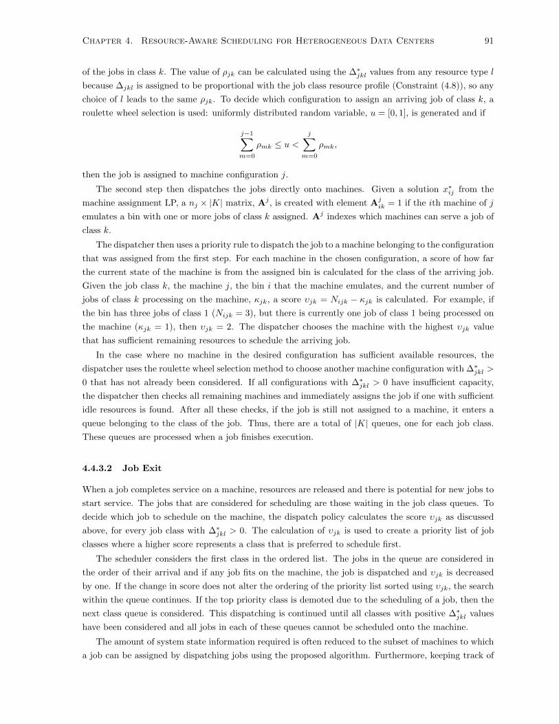
Chapter 4. Resource-Aware Scheduling for Heterogeneous Data Centers 91
of the jobs in class k. The value of ρjk can be calculated using the ∆∗jkl values from any resource type l
because ∆jkl is assigned to be proportional with the job class resource profile (Constraint (4.8)), so any
choice of l leads to the same ρjk. To decide which configuration to assign an arriving job of class k, a
roulette wheel selection is used: uniformly distributed random variable, u = [0, 1], is generated and if
j−1∑m=0
ρmk ≤ u <j∑
m=0
ρmk,
then the job is assigned to machine configuration j.
The second step then dispatches the jobs directly onto machines. Given a solution x∗ij from the
machine assignment LP, a nj × |K| matrix, Aj , is created with element Ajik = 1 if the ith machine of j
emulates a bin with one or more jobs of class k assigned. Aj indexes which machines can serve a job of
class k.
The dispatcher then uses a priority rule to dispatch the job to a machine belonging to the configuration
that was assigned from the first step. For each machine in the chosen configuration, a score of how far
the current state of the machine is from the assigned bin is calculated for the class of the arriving job.
Given the job class k, the machine j, the bin i that the machine emulates, and the current number of
jobs of class k processing on the machine, κjk, a score υjk = Nijk − κjk is calculated. For example, if
the bin has three jobs of class 1 (Nijk = 3), but there is currently one job of class 1 being processed on
the machine (κjk = 1), then υjk = 2. The dispatcher chooses the machine with the highest υjk value
that has sufficient remaining resources to schedule the arriving job.
In the case where no machine in the desired configuration has sufficient available resources, the
dispatcher uses the roulette wheel selection method to choose another machine configuration with ∆∗jkl >
0 that has not already been considered. If all configurations with ∆∗jkl > 0 have insufficient capacity,
the dispatcher then checks all remaining machines and immediately assigns the job if one with sufficient
idle resources is found. After all these checks, if the job is still not assigned to a machine, it enters a
queue belonging to the class of the job. Thus, there are a total of |K| queues, one for each job class.
These queues are processed when a job finishes execution.
4.4.3.2 Job Exit
When a job completes service on a machine, resources are released and there is potential for new jobs to
start service. The jobs that are considered for scheduling are those waiting in the job class queues. To
decide which job to schedule on the machine, the dispatch policy calculates the score υjk as discussed
above, for every job class with ∆∗jkl > 0. The calculation of υjk is used to create a priority list of job
classes where a higher score represents a class that is preferred to schedule first.
The scheduler considers the first class in the ordered list. The jobs in the queue are considered in
the order of their arrival and if any job fits on the machine, the job is dispatched and υjk is decreased
by one. If the change in score does not alter the ordering of the priority list sorted using υjk, the search
within the queue continues. If the top priority class is demoted due to the scheduling of a job, then the
next class queue is considered. This dispatching is continued until all classes with positive ∆∗jkl values
have been considered and all jobs in each of these queues cannot be scheduled onto the machine.
The amount of system state information required is often reduced to the subset of machines to which
a job can be assigned by dispatching jobs using the proposed algorithm. Furthermore, keeping track of
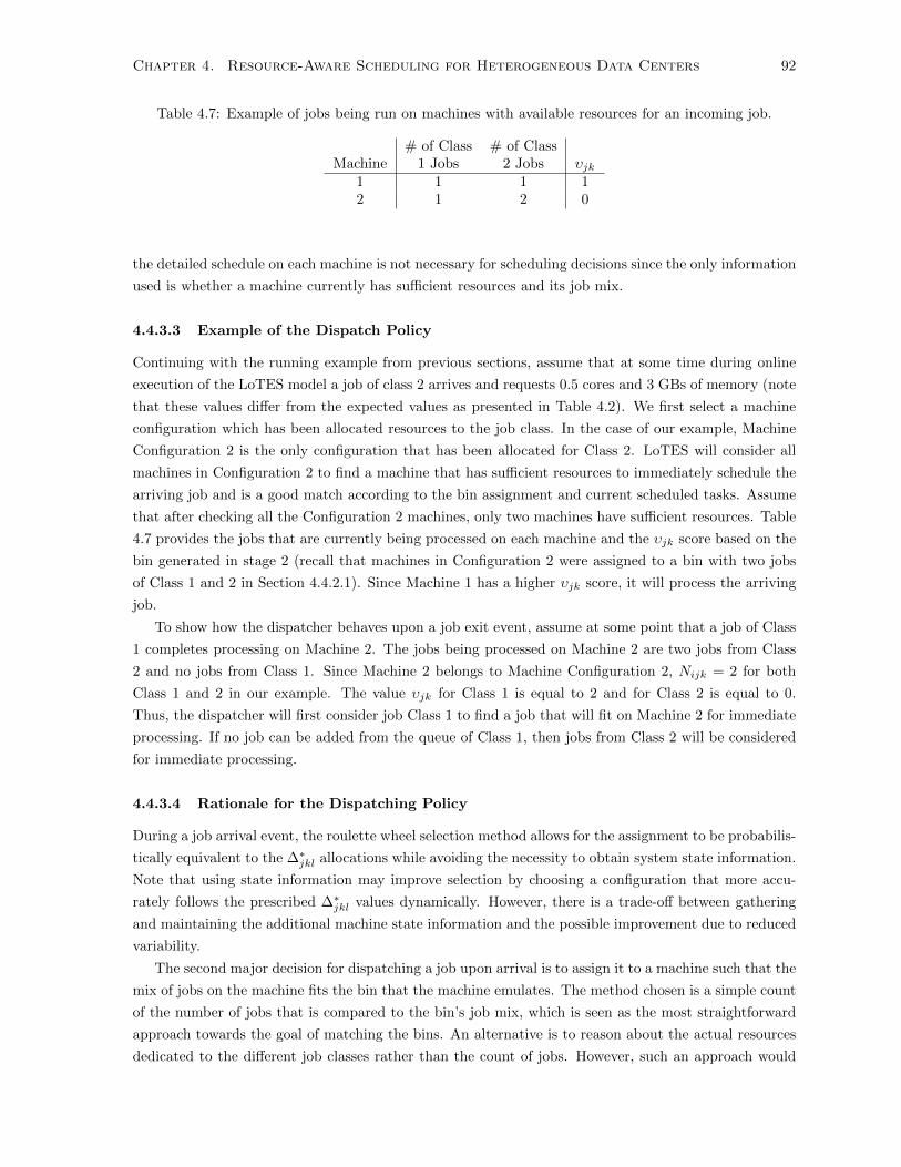
Chapter 4. Resource-Aware Scheduling for Heterogeneous Data Centers 92
Table 4.7: Example of jobs being run on machines with available resources for an incoming job.
# of Class # of ClassMachine 1 Jobs 2 Jobs υjk
1 1 1 12 1 2 0
the detailed schedule on each machine is not necessary for scheduling decisions since the only information
used is whether a machine currently has sufficient resources and its job mix.
4.4.3.3 Example of the Dispatch Policy
Continuing with the running example from previous sections, assume that at some time during online
execution of the LoTES model a job of class 2 arrives and requests 0.5 cores and 3 GBs of memory (note
that these values differ from the expected values as presented in Table 4.2). We first select a machine
configuration which has been allocated resources to the job class. In the case of our example, Machine
Configuration 2 is the only configuration that has been allocated for Class 2. LoTES will consider all
machines in Configuration 2 to find a machine that has sufficient resources to immediately schedule the
arriving job and is a good match according to the bin assignment and current scheduled tasks. Assume
that after checking all the Configuration 2 machines, only two machines have sufficient resources. Table
4.7 provides the jobs that are currently being processed on each machine and the υjk score based on the
bin generated in stage 2 (recall that machines in Configuration 2 were assigned to a bin with two jobs
of Class 1 and 2 in Section 4.4.2.1). Since Machine 1 has a higher υjk score, it will process the arriving
job.
To show how the dispatcher behaves upon a job exit event, assume at some point that a job of Class
1 completes processing on Machine 2. The jobs being processed on Machine 2 are two jobs from Class
2 and no jobs from Class 1. Since Machine 2 belongs to Machine Configuration 2, Nijk = 2 for both
Class 1 and 2 in our example. The value υjk for Class 1 is equal to 2 and for Class 2 is equal to 0.
Thus, the dispatcher will first consider job Class 1 to find a job that will fit on Machine 2 for immediate
processing. If no job can be added from the queue of Class 1, then jobs from Class 2 will be considered
for immediate processing.
4.4.3.4 Rationale for the Dispatching Policy
During a job arrival event, the roulette wheel selection method allows for the assignment to be probabilis-
tically equivalent to the ∆∗jkl allocations while avoiding the necessity to obtain system state information.
Note that using state information may improve selection by choosing a configuration that more accu-
rately follows the prescribed ∆∗jkl values dynamically. However, there is a trade-off between gathering
and maintaining the additional machine state information and the possible improvement due to reduced
variability.
The second major decision for dispatching a job upon arrival is to assign it to a machine such that the
mix of jobs on the machine fits the bin that the machine emulates. The method chosen is a simple count
of the number of jobs that is compared to the bin’s job mix, which is seen as the most straightforward
approach towards the goal of matching the bins. An alternative is to reason about the actual resources
dedicated to the different job classes rather than the count of jobs. However, such an approach would

Chapter 4. Resource-Aware Scheduling for Heterogeneous Data Centers 93
require modeling the variance of resource requirements and developing a more complicated measure of bin
emulation. Not only must one consider the realized resource requirements of jobs in the system, but one
can also account for the information regarding future job arrivals and the stochasticity in their resource
requirements as well. As there is no obvious way forward in this direction, the more straightforward
approach is used.
Finally for the job arrival event, all other configurations are checked before allowing a job to enter the
queue because doing so allows for the exploitation of idle resources, even if they deviate from the guidance
of the offline solutions. Such a deviation is beneficial because the presence of idle resources means the
system is likely to be in a lower load state, where responding to jobs immediately is more important
than long-term efficiency. During preliminary experiments, it was found that allowing these deviations
improved performance during times where the system was lightly loaded and did not negatively effect
performance during heavily loaded times. This policy attempts to schedule jobs immediately whenever
possible to reduce response times, while biasing towards placing jobs in such a way as to mimic the bins,
which aims to reduce the effects of resource fragmentation as the bins generated are non-dominated bins.
The proposed policy does not preclude the assignment of a pairing between a job class and machine
configuration with ∆∗jkl = 0 when the system is heavily loaded. When a job arrives, if at least one
machine can serve the job immediately, it will do so, regardless of the overall system load. In contrast,
once a job enters a queue, it will only be assigned to a machine with ∆∗jkl > 0. This strategy may
leave machines idle as the system load decreases and machines become available, but the jobs in the
queue continue to wait for heavily contended machines. The reasoning regarding when one should switch
strategies is not clear and so the policy presented aims to simplify this decision by assuming that any
time a machine has free resources upon a job arrival, the scheduler treats the system as though it were
lightly loaded. A more nuanced approach may improve system performance, but is not explored in
detail.
The rationales for the choices in the job exit event are similar to the job arrival choices. By using a
count of how the actual mix of jobs deviates from the emulated bin, the policy more closely mimics the
chosen bin. Unlike the job arrival event, the choice of not scheduling any job classes with ∆jkl = 0 is
made since the system is likely heavily loaded (a queue has formed) and pairing efficiency has increased
importance to improve system throughput. Therefore, it is possible that LoTES leaves a machine’s
resources idle even though a job in a queue with ∆jk = 0 can fit on the machine because it is likely
better to reserve those resources for a more efficient matching.
4.5 Experimental Results
The algorithm is tested on real cluster workload trace data and on generated data. In this section, details
of the experiments are provided. The implementation challenges are discussed, followed by a description
and presentation of the results for the algorithms on the workload trace data and the generated data.
4.5.1 Implementation Challenges
In these experiments, the time it takes for the scheduler to make dispatching decisions is not considered.
As such, as soon as a job arrives to the system and at least one machine has sufficient idle resources,
it is assumed that the schedule assigns it to a machine with zero elapsed time. In practice, decisions
are not instantaneous and, depending on the information needed by the scheduler and the complexity of

Chapter 4. Resource-Aware Scheduling for Heterogeneous Data Centers 94
the scheduling algorithm, this delay may be an issue. For every new job arrival, the scheduler requires
the currently available resources. As the system becomes busier, the scheduler may have to obtain such
information for all machines in the data center. Thus, scaling may be problematic as the algorithms may
have to search over a very large number of machines. However, in heavily loaded systems where there
are delays before a job can start processing, the scheduling overhead does not adversely affect system
performance as the waiting time delays of jobs are orders of magnitude larger than the processing time.
Additionally, the scheduler itself creates load on the network connections within the data center. This
issue may need to be accounted for if the network connections become sufficiently congested.
However, the dispatching overhead of arriving jobs for LoTES is no worse than that of the Greedy
policy or Tetris. The LoTES algorithm benefits from the restricted set of machines that it considers
based on the ∆∗jkl values. At low loads where a job can be dispatched immediately as it arrives, the
Greedy policy and LoTES do not have to gather state information for all machines. In contrast, the
Tetris scheduler always gathers information on all machines to decide which has the best score. However,
in the worst case, LoTES may require state information on every machine when the system is heavily
loaded, just as the other algorithms.
A system manager for a very large data center must take into account the overhead required to
obtain machine state information regardless of which algorithm is chosen. There is work showing the
benefits of only sampling state information from a limited set of machines to make a scheduling decision
[117]. If the overhead of obtaining state information is problematic, one can further limit the number
of machines to be considered once a configuration has already been chosen. Such a scheduler could
decide which configuration to send an arriving job to and then sample N machines randomly from the
chosen configuration, where N ∈ [1, nj ]. The scheduler can then dispatch jobs following the same rules
as LoTES, allowing the mappings from the offline stages of LoTES to still be used but with substantially
less overhead for the online decisions.
4.5.2 Google Workload Trace Data
The first experiment uses cluster workload trace data provided by Google.11 These data represent
the workload for one of Google’s compute clusters over the one month period of May 2011, providing
information on the machines in the system as well as the jobs that arrive, their submission times, their
resource requests, and their durations, which can be inferred from the time for which a job is active.
However, because calculation of the processing time of a job is based on the actual processing time
realized in the workload traces, it is not known here how processing times may have differed if a job were
to be processed on a different machine or if the load on the machine were to be different. Therefore,
processing times are assumed to be independent of machine configuration and load.12
Although the information provided is extensive, what is used for the experiments is limited to only
the resources requested and duration for each job. The failures of machines or jobs are not considered:
jobs that fail and are resubmitted are considered to be new, unrelated jobs. Figure 4.5 shows the number
of jobs arriving during each hour for the entire month of the trace data. Machine configurations change
over time due to failures, the acquisition of new servers, or the decommissioning of old ones, but only the
initial set of machines are used and is kept constant over the whole month. Furthermore, system micro-
architecture is provided for each machine and some jobs are limited in which types of architecture they
11The data can be found at https://code.google.com/p/googleclusterdata/.12The impact of processing time variation is examined in subsequent experiments (see Section 4.5.3.3).

Chapter 4. Resource-Aware Scheduling for Heterogeneous Data Centers 95
0
20000
40000
60000
80000
100000
120000
140000
160000
180000
0 100 200 300 400 500 600 700
Num
ber o
f Job
Arri
vals
Time (h)
Figure 4.5: The number of jobs arriving in each hour in the Google workload trace data.
can be paired with and how they interact with these architectures. This limitation is ignored for these
scheduling experiments. It is easy to extend the LoTES algorithm to account for system architecture by
setting µjk = 0 whenever a job cannot be processed on a particular architecture.
4.5.2.1 Machine Configurations
The data center has 10 machine configurations as presented in Table 4.8. Each configuration is defined
strictly by its resource capacities and the number of identical machines with that resource profile. The
resource capacities are normalized relative to the configuration with the most resources. Therefore, the
job resource requests are also provided after being normalized to the maximum capacity of machines.
4.5.2.2 Job Class Clustering
The Google data does not define job classes and so to use the data for LoTES, one must first cluster jobs
into classes. Following Mishra et al. [175], k-means clustering is used to create job classes. Specifically,
Lloyd’s algorithm [161] is used to create the different clusters. To limit the amount of information that
LoTES uses in comparison to the benchmark algorithms, only the jobs from the first day are used to
define the job classes for the month. These classes are assumed to be fixed for the entire month. Due to
this assumption and because the Greedy policy and the Tetris scheduler do not use class information,
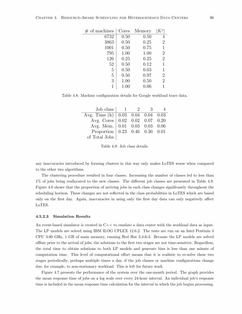
Chapter 4. Resource-Aware Scheduling for Heterogeneous Data Centers 96
# of machines Cores Memory |Kj|6732 0.50 0.50 43863 0.50 0.25 21001 0.50 0.75 1795 1.00 1.00 2126 0.25 0.25 252 0.50 0.12 15 0.50 0.03 15 0.50 0.97 23 1.00 0.50 21 1.00 0.06 1
Table 4.8: Machine configuration details for Google workload trace data.
Job class 1 2 3 4Avg. Time (h) 0.03 0.04 0.04 0.03
Avg. Cores 0.02 0.02 0.07 0.20Avg. Mem. 0.01 0.03 0.03 0.06Proportion 0.23 0.46 0.30 0.01
of Total Jobs
Table 4.9: Job class details.
any inaccuracies introduced by forming clusters in this way only makes LoTES worse when compared
to the other two algorithms.
The clustering procedure resulted in four classes. Increasing the number of classes led to less than
1% of jobs being reallocated to the new classes. The different job classes are presented in Table 4.9.
Figure 4.6 shows that the proportion of arriving jobs in each class changes significantly throughout the
scheduling horizon. These changes are not reflected in the class probabilities in LoTES which are based
only on the first day. Again, inaccuracies in using only the first day data can only negatively affect
LoTES.
4.5.2.3 Simulation Results
An event-based simulator is created in C++ to emulate a data center with the workload data as input.
The LP models are solved using IBM ILOG CPLEX 12.6.2. The tests are run on an Intel Pentium 4
CPU 3.00 GHz, 1 GB of main memory, running Red Hat 3.4-6-3. Because the LP models are solved
offline prior to the arrival of jobs, the solutions to the first two stages are not time-sensitive. Regardless,
the total time to obtain solutions to both LP models and generate bins is less than one minute of
computation time. This level of computational effort means that it is realistic to re-solve these two
stages periodically, perhaps multiple times a day, if the job classes or machine configurations change
due, for example, to non-stationary workload. This is left for future work.
Figure 4.7 presents the performance of the system over the one-month period. The graph provides
the mean response time of jobs on a log scale over every 24-hour interval. An individual job’s response
time is included in the mean response time calculation for the interval in which the job begins processing.

Chapter 4. Resource-Aware Scheduling for Heterogeneous Data Centers 97
0
0.1
0.2
0.3
0.4
0.5
0.6
0.7
0.8
0.9
1
0 5 10 15 20 25
Prop
ortio
n of
Arr
ival
s
Day
Job Class 1Job Class 2Job Class 3Job Class 4
Figure 4.6: Daily proportion of jobs belonging to each job class.
The LoTES algorithm greatly outperforms the Greedy policy and generally has lower response times
than Tetris. On average, the Greedy policy has response times that are orders of magnitude longer
(15-20 minutes) than the response times of the LoTES algorithm. The Tetris scheduler performs much
better than the Greedy policy, but still has about an order of magnitude longer response times than
LoTES.
The overall performance shows the benefits of LoTES, however, a more interesting result is the
performance difference when there is a larger performance gap between the scheduling algorithms. In
general, LoTES is as good as Tetris or better. However, when the two algorithms deviate in performance,
LoTES can perform significantly better. For example, around the 200 hour time point in Figure 4.7, the
average response time of jobs is minutes with the Greedy policy, seconds under Tetris, and micro-seconds
with LoTES.
The Greedy policy performs worst as it is the most myopic. However, the one time period that it
does exhibit better behavior than any other scheduler is the first period when the system is in a highly
transient state and is heavily loaded. This is believed to be due to the scheduler being myopic and
optimizing for the immediate time period which leads to better short-term results, but the performance
then degrades over a longer time horizon.
Although it is shown in Figure 4.7 that LoTES can reduce the response times of jobs, the large scale
of the system obscures the significance of even these seemingly small time improvements between LoTES
and Tetris. Often, the difference in average response times for these two schedulers is tenths of seconds
(or even smaller). When examining the distribution of response times from Figure 4.8, Tetris has a
much larger tail where more jobs have a significantly slower response time. For the LoTES scheduler,
less than 1% of jobs have a waiting time greater than one hour. In comparison, the Tetris scheduler has

Chapter 4. Resource-Aware Scheduling for Heterogeneous Data Centers 98
1e-12
1e-10
1e-08
1e-06
0.0001
0.01
1
100
0 100 200 300 400 500 600 700
Mea
n Re
spon
se T
ime
(h)
Time (h)
GreedyTetrisLoTES
Figure 4.7: Response Time Comparison.
just as many jobs that have a waiting time greater than seven hours and the Greedy policy has 1% of
jobs waiting longer than 17 hours. These values show how poor performance can become during peak
times, even though on average, the response times are very short because the vast majority of jobs are
immediately processed.
Finally, Figure 4.9 presents the number of jobs in queue over time. For most of the month, the
queue size does not grow to any significant degree for LoTES. Tetris does have a queue form at some
points in the month, but even then, the queue length is relatively small. Other than at the beginning of
the schedule, the throughput of jobs for Tetris and LoTES is generally maintained at a rate such that
arriving jobs are processed immediately. The large burst of jobs early on in the schedule is due to the
way in which the trace data was captured: all these jobs enter the system at the beginning as a large
batch to be scheduled. However, as time goes on, these initial jobs are processed and the system enters
into more regular operation. The Greedy policy on the other hand has increased queue lengths at all
points during the month.
Given that, for the majority of the scheduling horizon, LoTES is able to maintain empty queues
and schedule jobs immediately, a scheduling decision can often be made by considering only a subset
of machine configurations rather than all machines in the system. In contrast, the Tetris scheduler,
regardless of how uncongested the system is, always considers all machines to find the best score. The
scheduling overhead is not presented, but it is apparent from the graph that without a queue build up,
the overhead of LoTES is no worse, and is more likely better, than Tetris.
It is important to state here again that LoTES makes use of additional job class information, which
is not considered by the other schedulers. However, the information can be inaccurate as seen in Figure
4.6, where the proportion of arriving jobs belonging to a job class can be seen to change over time. One
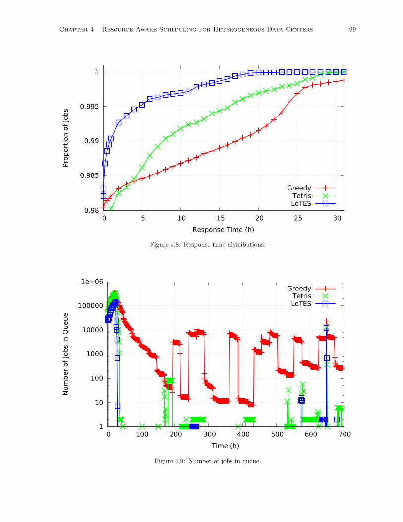
Chapter 4. Resource-Aware Scheduling for Heterogeneous Data Centers 99
0.98
0.985
0.99
0.995
1
0 5 10 15 20 25 30
Prop
ortio
n of
Jobs
Response Time (h)
GreedyTetrisLoTES
Figure 4.8: Response time distributions.
1
10
100
1000
10000
100000
1e+06
0 100 200 300 400 500 600 700
Num
ber o
f Job
s in
Que
ue
Time (h)
GreedyTetrisLoTES
Figure 4.9: Number of jobs in queue.

Chapter 4. Resource-Aware Scheduling for Heterogeneous Data Centers 100
would expect that improvements could be made by dynamically updating the parameters of the job
classes to ensure that LoTES maintains an accurate representation of the system. Regardless, even with
a fairly naive approach where the job classes are assumed to be static, the LoTES scheduler is able to
perform well.
4.5.3 Randomly Generated Workload Trace Data
Randomly generated data is used to show the behavior of LoTES when varying the resource requirements
of job classes and when including machine dependent processing times.
In two experiments, nine job classes are created that all arrive at the same rate αλ, where α = 19
and λ is the total arrival rate of the system. Jobs arrive following a Poisson process with exponentially
distributed inter-arrival times. Each job, z, has an amount of work, wz, that must be done, which is
generated from an exponential distribution with mean 1. The work is used to define the processing time,
which is pz = wzµjk
given that job z is a job of class k and is processed on a machine of configuration j. To
generate the resource requirements of a job, a randomly generated value following a truncated Gaussian
distribution with mean rkl, coefficient of variation 0.5 for class k and resource l, and truncated to be in
the interval [0, 1], is obtained for each resource l ∈ R.
4.5.3.1 Machine Configurations
The same machine configurations from the Google workload trace data in Table 4.8 are used, except the
total number of machines in each configuration are changed to 1000 machines per configuration so that
the system is more equally balanced between the different types of configurations available. Although
balancing the configurations is not crucial, it is done to emphasize the heterogeneity of machines; more
specifically, it is preferable to avoid having one or two configurations that represent the majority of all
machines in the system.
4.5.3.2 Job Class Details: Varying Resource Requirements
The first set of generated data varies the resource requirements for different classes. A range of sys-
tems are considered, starting with one where all nine job classes have the same resource requirement
distribution and progressively increasing the differences between the job classes.
Let parameter Φ denote the measure of the difference in resource requirements of job classes. Given
some value Φ, a value for each job class and resource pair φkl = U [−Φ,Φ] is randomly generated following
a uniform distribution. Jobs from class k then has resource requirements generated from a truncated
Gaussian distribution with mean rkl = 0.025 +φkl, coefficient of variation of 0.5, and truncated to be in
[0,1]. As Φ grows, a larger difference between the resource requirements of jobs between different classes
is expected. When Φ = 0, all job classes have the same resource requirement distribution.
An arrival rate of λ = 0.97λ∗ is chosen, where λ∗ is the solution of the machine assignment LP.
This load represents a heavily utilized system that is, from preliminary experiments, still stable for
LoTES and Tetris.13 However, the Greedy policy is not stable at this arrival rate: queue sizes increase
unboundedly with time. Therefore, only the results for LoTES and Tetris are shown.
13Note that λ∗ represents an upper bound on the system load that can be handled. The bound may not be tightdepending on the fragmentation of resources on a machine and/or the inefficiencies in the scheduling model used.

Chapter 4. Resource-Aware Scheduling for Heterogeneous Data Centers 101
0.0001
0.001
0.01
0.1
1
0 0.002 0.004 0.006 0.008 0.01 0.012 0.014 0.016
Mea
n Re
spon
se T
ime
(h)
Φ
TetrisLoTES
Figure 4.10: Results for varying resource requirements between job classes.
Simulations are done for values of Φ between 0 and 0.015, in increments of 0.003. Thus, the systems
tested range from one where all mean resource requirements are 0.025 regardless of job class or resource,
to one that can have average resource requirements ranging from 0.01 to 0.04. The processing rate is
generated by first obtaining a uniformly distributed random value uk = U [0, 1] for each job class k,
and setting µjk = u−1k for all machine configurations j. For each value of Φ, five different instances
are created, by generating rkl and uk values independently, and simulating the system for 1000 hours.
The mean response time for all jobs in the 1000 hour simulation is recorded and the mean over the five
instances for each tested Φ is presented in Figure 4.10.
When Φ = 0, all job classes are the same and both scheduling algorithms yield short response times.
Due to the logarithmic scaling of the graph, the apparent difference is actually insignificant.
As Φ increases, both scheduling algorithms have longer response times. This is believed to be due
to the fact that the maximum system load, λ∗, becomes looser as Φ grows due to fragmentation and
wasted resources. This issue is further exacerbated by the inefficiencies in scheduling that decrease the
throughput of machines, effectively increasing the system load. Thus, both scheduling models have
longer response times when Φ > 0, and Tetris becomes much worse than LoTES. LoTES takes better
advantage of efficient packing of jobs onto machines using the allocation LP and machine assignment
LP solutions.
4.5.3.3 Job Class Details: Varying Processing Time
The second set of generated data considered looks at processing times that are dependent on the ma-
chine configuration. For these experiments, the resource requirements, rkl, generated from the previous
experiment with Φ = 0.06 are used. Rather than using a random value uk to obtain the processing

Chapter 4. Resource-Aware Scheduling for Heterogeneous Data Centers 102
0
0.2
0.4
0.6
0.8
1
1.2
1.4
1.6
0 0.05 0.1 0.15 0.2 0.25 0.3
Mea
n Re
spon
se T
ime
(h)
Ω
TetrisLoTES
Figure 4.11: Results for varying resource requirements between job classes. System load of 0.90.
rate, an additional value ωjk, a multiplier that makes the processing rate dependent on the machine
configuration, is used. Given some value Ω, ωjk is randomly generated from a uniform distribution
U [1−Ω, 1 + Ω] for each machine configuration j and job class k. The processing rate is then calculated
as µjk = ukωjk.
A range of Ω values is tested to observe how the scheduling models behave as the system is changed
from a system with machine-configuration-independent processing times to ones with increased machine
configuration dependency. As before, five instances are generated for each value of Ω where the same rkl
values from the previous experiment, but generate ωjk independently for each instance. A simulation
time of 1000 hours is performed and the mean response time is recorded.
Two different system loads are used: 0.90 and 0.95. Both these loads are chosen to be lower than
in the previous experiment as it was found in preliminary experiments that a load of 0.97 often led to
instability in the system. Figures 4.11 and 4.12 show the system performance with loads of 0.90 and
0.95, respectively. Results for Greedy are not presented as at these loads, the system is not stable. At
a load of 0.95, Tetris also appears to be unstable at higher values of Ω and thus response times are only
reported for Ω ≤ 0.1.
At a load of 0.90, LoTES is essentially able to start all jobs immediately. In comparison, Tetris is
able to start all jobs immediately when Ω = 0, but a continual increase in the average response time is
observed as Ω increases, as scheduling inefficiencies result in a drastic reduction of system throughput.
To illustrate the performance of LoTES with increased Ω, a system load of 0.95 is tested so that LoTES
is no longer able to immediately start all jobs. Similar to Tetris, a rapid growth in response time with
Ω is observed. It is suspected that the reason that LoTES outperforms Tetris on these experiments is
due to its ability to find efficient allocations that take into account the trade-off between processing time

Chapter 4. Resource-Aware Scheduling for Heterogeneous Data Centers 103
0
0.05
0.1
0.15
0.2
0.25
0.3
0.35
0.4
0 0.1 0.2 0.3 0.4 0.5
Mea
n Re
spon
se T
ime
(h)
Ω
TetrisLoTES
Figure 4.12: Results for varying resource requirements between job classes. System load of 0.95.
dependencies and fragmentation due to job mixes. Tetris also considers processing time dependencies
and job fragmentation, but does so greedily by prioritizing low processing time allocations and best-
fits of the resource requirements rather than efficient mixes. Incorporating longer term reasoning that
considers the system performance rather than the job performance means that the LoTES algorithm is
better equipped to handle varied processing times as it can make informed decisions on a set of jobs.
4.5.4 Impact of the Offline Stages of LoTES
Here, the impact of the first two stages of LoTES is studied. In particular, an exploration of what
happens when either the first or second stage is removed is performed.
4.5.4.1 Removing the First Stage of LoTES
In order to remove the first stage of the LoTES scheduler (the allocation LP), the second stage must
be updated, as it no longer has access to the δ∗jkl values that restrict the bin configurations generated
in the second stage. Without the guidance from the allocation LP, all potential job class and machine
configuration pairings must be considered, which leads to an increase in the number of bins generated.
However, removing the first stage also provides the machine assignment LP access to many more bin
choices which may improve performance over the standard LoTES scheduler.
4.5.4.2 Removing the Second Stage of LoTES
Removal of the second stage is a more involved process as it is responsible for generating bins and
providing the third stage dispatcher with its scheduling policy. Now, instead of machine assignments to

Chapter 4. Resource-Aware Scheduling for Heterogeneous Data Centers 104
bins, only the allocation LP δ∗jkl values are used to provide dispatching guidance.
Upon job arrival into the system, the dispatcher chooses a machine configuration similarly to the
standard LoTES scheduler using a roulette wheel selection method, but uses δ∗jkl rather than ∆∗jkl.
Within the machine configuration, the dispatcher searches through the machines in an arbitrary order
and schedules the job on the first machine that has sufficient resources available. If no machines are
available, another configuration is chosen. This process continues until the job is either scheduled or all
machines have been considered and the job enters a queue belonging to the job class.
When a job is completed on a machine and resources become free, the dispatcher follows the same
steps as the standard LoTES scheduler except for the decision on which job class to consider. Rather
than use the bin configurations to guide job class selection, the roulette wheel selection method is used
with the δ∗jkl values as weights.
4.5.4.3 Simulation Results
To study the effects of removing the first and second stages, the system is simulated with generated data
and three schedulers are compared: LoTES, NoFirst, and NoSecond. The machine configurations used
in these experiments are the same as those used in the previous randomly generated workload data, but
the job classes are from the Google workload trace data, which consists of four job classes. The result
is a system based on the Google workload trace data, but with a larger emphasis on having different
machine configurations that make up a significant portion of the data center.
A parameter Υ, that signifies the relative machine capacities, is introduced to understand the behavior
of the LoTES variations as the total capacity of the machines in the system is altered. Given some
baseline values for the capacity of resource l on machine configuration j, denoted bjl, systems where the
resource capacity is cjl = Υbjl are tested. The machine capacity is varied as an independent variable
because of the way that capacity interacts with bin generation and fragmentation - key aspects that
the first two stages have impact on. Machines with larger capacities have many more bins that they
may emulate. As the first stage regulates the pairings of job classes and machines, it is important when
one must deal with the combinatorial explosion of the number of bins generated. Alternatively, smaller
capacity machines will likely increase the effect of fragmentation as, in the limit as the capacity of the
machines increase, job resource requirements become relatively small and can be treated as a fluid. The
second stage is better equipped to deal with fragmentation than the first stage, and it is believed to be
necessary for obtaining high performance in systems with machine low capacity. Thus, it is expected to
see NoFirst perform well compared to LoTES and NoSecond when Υ is small, but as Υ increases, the
performance of the three schedulers should converge. However, increasing Υ will lead to a much faster
growth rate of generated bins, potentially crippling NoFirst as the generation of bins and solving of the
machine assignment LP becomes intractable.
Figure 4.13 presents the results of the simulation. The resource capacities of the machines from
Table 4.8 are used as a baseline and we perform simulations for Υ values from 1 to 3 in increments of
0.1. The experiments are simulations of the data center for 1000 hours for each Υ value. The mean
response time is calculated based on all jobs over the 1000 hour simulation time. NoFirst performs best
overall, with LoTES in the middle and NoSecond worst. For all variations, the computational effort of
the offline stages is low, with LoTES and NoSecond requiring on the order of one-hundredth of a second
and NoFirst requiring on the order of one-tenth of a second.
NoFirst performs better than LoTES because it does not include the restrictions of a subset of

Chapter 4. Resource-Aware Scheduling for Heterogeneous Data Centers 105
0
0.02
0.04
0.06
0.08
0.1
0.12
0.14
1 1.5 2 2.5 3
Mea
n Re
spon
se T
ime
(h)
Υ
NoSecondLoTES
NoFirst
Figure 4.13: Simulation results for LoTES variations with removed first and second stages.
job classes to machine configurations. Without the restrictions, NoFirst uses a superset of bins in the
machine assignment LP that can lead to better bin assignments. However, without restrictions, the
number of bins generated can lead to an intractable model. Figure 4.14 illustrates the total number of
bins generated for NoFirst and LoTES.
In these experiments, there are few job classes (four), however, a data center with more job classes or
larger capacities leads to an exponential increase in the number of bins generated. To show the necessity
of the first stage in systems with a larger number of job classes, the number of bins generated and the
runtime for the offline stages of LoTES and NoFirst are plotted in Figures 4.15 and 4.16, respectively.
Here, Υ = 1 is used and the job classes from the Google workload trace data is duplicated to create new
job classes. The number of generated bins quickly increases into the millions for the NoFirst model and
no solution can be found past nine job classes after a one-hour time-limit. When Υ = 2 is tested, time-
out occurs after six job classes with 3.7 million bins generated. Thus, although the best performer as
indicated by the simulations is NoFirst, it will not be tractable, even offline, for more than approximately
six to nine job classes, depending on machine capacities. It is crucial to ensure that the scheduler used
is tractable since a time-out means that the second stage will not have a complete set of bins and so
is useless given that even a sub-optimal solution to the machine assignment is not available for use in
the third stage. Including the allocation LP to restrict the bin generation ensures solvability while still
outperforming the benchmark scheduling algorithms.

Chapter 4. Resource-Aware Scheduling for Heterogeneous Data Centers 106
0
20000
40000
60000
80000
100000
120000
140000
160000
1 1.5 2 2.5 3
Num
ber o
f Bin
s
Υ
NoFirstLoTES
Figure 4.14: Number of bins generated for the data center.
0
500000
1e+06
1.5e+06
2e+06
2.5e+06
3e+06
3.5e+06
4e+06
4 5 6 7 8 9
Num
ber o
f Bin
s
Number of Job Classes
NoFirstLoTES
Figure 4.15: Number of bins generated for the data center.

Chapter 4. Resource-Aware Scheduling for Heterogeneous Data Centers 107
0
10
20
30
40
50
60
70
80
90
4 5 6 7 8 9
Runt
ime
of O
ine
Stag
es (s
)
Number of Job Classes
NoFirstLoTES
Figure 4.16: Running time for the offline stages of the scheduler.
4.6 Discussion
The empirical results from the simulations show the advantages of the LoTES model in comparison to
the benchmark scheduling algorithms. In this section, the LoTES decomposition and the benefits due
to combining queueing theory and scheduling is presented. A discussion of future directions for this
research is then provided.
4.6.1 Decomposition: Benefits and Insights
The main advantage of the LoTES decomposition comes from the combination of the two fields of
queueing theory and combinatorial scheduling. Through a decomposition, it is possible to relax the
problem by introducing abstractions such that the resulting relaxation is more amenable to the technique
chosen at each stage. The result is a scheduler that can take into account both the dynamism of the
system through queueing theory and the combinatorics through scheduling.
Although the decomposition as presented can be altered and high performance is still obtainable (see
Figure 4.13), there are clear benefits of including all stages (see Figures 4.15 and 4.16). The first stage
greatly restricts the size of the combinatorial problem that is to be considered in the second phase, while
doing so in an intelligent manner that does not hurt performance greatly.
The framework of the LoTES scheduler can be generalized to a larger class of systems than just
data centers. The decomposition takes the approach of first representing the dynamism of the problem
through a queueing model, solving a combinatorial scheduling problem guided by the results of the
queueing model, and then re-solving a variation of the queueing model based on constraints from the
combinatorial optimization. The idea of combining queueing theory and scheduling, while not new, is

Chapter 4. Resource-Aware Scheduling for Heterogeneous Data Centers 108
not well studied in the literature. Similar models can be found that make use of an allocation LP first,
followed by a combinatorial scheduling phase [233, 237]. A key commonality between those systems
and the data center scheduling problem is the large impact on system performance due to job routing
decisions. An efficient routing can significantly improve performance and may be the difference between a
stable or unstable system [8, 77]. Thus, one should consider the system dynamics when making decisions.
Yet, studying only the dynamics of the system can be insufficient due to combinatorial effects such as
fragmentation. In dynamic systems with both a routing and scheduling component, the decomposition
approach as presented in this chapter is a suitable candidate. The framework of a queueing model (in the
form of an allocation LP) and a scheduling model (guided by the allocation LP) can be applied to many
systems, so long as the appropriate changes to the allocation LP are made and a relevant scheduling
model is defined.
The LoTES framework can also be extended to consider large complex systems that does not have
dynamic characteristics. As seen in Section 4.5.4, the allocation LP helped to greatly reduce the number
of bins that were generated. One could update the allocation LP to consider the amount of work in
a static system, solve the fluid representation of this system with an LP and use the results from the
LP to restrict the search space for a combinatorial scheduling model. Doing so loses completeness, but
for very large problems, such an approach can help make intractable problems manageable without too
much loss in performance.
4.6.2 Future Work
The data center scheduling problem is very rich from the scheduling perspective and the proposed
approach can be expanded in a number of ways. The proposed algorithm assumes stationary arrivals
over the entire duration of the scheduling horizon. However, the real system is not stationary and the
arrival rate of each job class may vary over time. Furthermore, the actual job classes themselves may
change over time as resource requirements may not always be clustered in the same manner. As noted,
the offline phase is sufficiently fast (less than one second of CPU time) that it could be run multiple times
per day as the system and load characteristics change. Although running the system in this manner
assumes that an accurate and updated model of the job classes is available so that the offline stages can
be run online. In practice, it may be non-trivial to cluster jobs in real-time in order to decide on job
classes. Thus the LoTES algorithm can be extended to more accurately represent dynamic job classes,
allowing LoTES to learn to predict the expected mix of jobs that arrives to the system and to make
scheduling decisions based on these predictions. Furthermore, the algorithm can also be made to more
intelligently handle situations when the mix of jobs varies greatly from the expectation. Large deviations
from the expectation lead to system realizations that differ significantly from the bins created in the
second stage of the LoTES algorithm and make the offline decisions less relevant to the realized system.
We also plan to study the effects of errors in job resource requests. In this study, the amount of
requested resources of a job is used as the amount of resource required over the entire duration of the
job. In reality, users may under or overestimate their resource requirements and the utilization of a
resource may change over the duration of the job itself. Uncertainties in resource usage add difficulty
to the problem because instead of knowing the exact amount of requested resources once a job arrives,
only an estimate is available and one must ensure that a machine is not underutilized or oversubscribed.
Finally, the literature on data center scheduling has considered various different objectives and con-
straints. Fairness among multiple users has been an important topic to ensure that the system not just

Chapter 4. Resource-Aware Scheduling for Heterogeneous Data Centers 109
responds quickly to job requests, but provides equal access to resources [129, 258]. Including fairness
considerations in LoTES is a possible future direction, which can be accomplished by either including
users in the LP models of the first two stages to ensure resources are shared, or by introducing priori-
tization for fairness in the dispatch policy of the third stage in a similar way to Delay scheduling [258].
Another important system aspect is energy consumption [38, 160]. Tarplee et al. [230] present a multi-
stage scheduling model similar to LoTES that directly considers energy consumption in a data center,
where jobs do not arrive dynamically over time (as they do in this system). Their scheduler uses an LP
relaxation with similar goals to ours in that it relaxes the problem to divide the load of a job across
multiple machines. The LP solution then is used to guide the scheduling choices. The minimization
of energy consumption is crucial for running low-cost data centers and is an important area for future
work.
4.7 Conclusion
In this chapter, the LoTES scheduling algorithm is developed, which improves response times for large-
scale data centers by creating a mapping between jobs and machines based on their resource profiles.
The algorithm consists of three stages:
1. A queueing model that uses a fluid representation of the system to allocate job classes to machine
configurations. This stage extends existing models in the queueing theory literature to include
multi-capacity resources and provides long-term stochastic knowledge by finding efficient pairings
of job classes and machine configurations that lead to maximizing system throughput for the
abstracted system.
2. A stage that assigns a particular job mix to each machine. The assignment is restricted by the
solution of the first stage in order to both reduce the combinations that are considered and to
incorporate the long-term view of the system. This stage treats jobs and machines as discrete
entities and performs combinatorial reasoning without losing the long-term knowledge.
3. A dispatching policy to realize the machine assignments made in the second stage. The primary
goal of this stage is to ensure that the system tends towards scheduling decisions that mimic the
prescribed assignments from Stage 2. However, the policy also aims to reduce response times by
actively deviating from the prescribed assignments when the system has idle resources. This stage
allows for the scheduling system to respond to the incoming arrival of tasks in a timely manner
while benefiting from the offline optimization.
The algorithm was tested on Google workload trace data and on randomly generated data, where
it was found to reduce response times by orders of magnitude when compared to a benchmark greedy
dispatch policy and by an order of magnitude when compared to the Tetris scheduler [109]. The main
advantage of LoTES over Tetris is that the former considers future job arrivals by generating efficient
bins in advance, which can then be mimicked by the machines online. LoTES behaves less myopically
and can reason about good packing efficiency based on combinations of jobs rather than a single job
at a time. This improvement is also computationally cheaper during the online scheduling phase since
LoTES often requires state information for fewer machines when making assignment decisions.

Chapter 5
A Quantum-Classical Approach to
Solving Scheduling Problems14
The focus of the previous two chapters was on decomposition models that are solved using classical
computing hardware. The weaknesses of different solvers are presented and through the use of a decom-
position, these shortcomings can be overcome. In this chapter, quantum computing, more specifically
quantum annealing, and its use within a classical/quantum decomposition framework is explored. The
deficiencies of the current quantum annealing hardware is examined and a decomposition which makes
use of classical and quantum computing to extend the applications where quantum technology can be
applied is presented.
5.1 Introduction
Quantum computing is a nascent technology without the decades of research and development that have
gone into classical computers. Current quantum computational hardware of more than several qubits
consists of only limited quantum annealers, special purpose quantum hardware designed to run the
quantum annealing metaheuristic [26, 43, 227]. Although one can reasonably expect that the hardware
will be improved to increase the number of qubits in the future, current quantum computers are not yet
capable of handling problems of a relevant scale to be of use.
The goal of the work in this Chapter is to extend the use of quantum annealing on currently available
specialized quantum hardware through integration with classical computing using decomposition. A
novel hybrid quantum-classical framework, based on tree search, is explored. The quantum annealer
samples from the configuration space of a relaxed problem to obtain strong candidate solutions, while
the classical algorithm maintains a global search tree, as well as handling the relaxed components of the
problem to check the validity and quality of the candidate solutions.
The proposed framework takes advantage of the strength of quantum hardware and complements
it with classical processing to enable the entire algorithm to be complete. The algorithm uses results
returned by the quantum annealer to guide the exploration and pruning of a search tree. Specifically,
the solution of samples of different parts of the solution space that are returned by the quantum annealer
are used to help guide search. A novel aspect of this work is that the approach makes use of all results
14The work in this chapter is based on work published at the Symposium on Combinatorial Search [236].
110

Chapter 5. A Quantum-Classical Approach to Solving Scheduling Problems 111
returned by the quantum annealer, not just the best ones as is common in the quantum annealing
community.
The decomposition is evaluated on three scheduling domains: graph coloring,15 Mars lander task
scheduling and airport runway scheduling. These three domains have varying complexity in their de-
compositions: (1) a decision problem that is fully represented on the quantum annealer, but using the
framework allows for a complete search, (2) a decision problem in which the quantum annealer samples
from the configuration space of a relaxation of the original problem, and (3) an optimization problem in
which the quantum annealer ignores the objective function and a classical computer is used instead to
handle the objective function.
This chapter provides a proof of concept quantum-classical hybrid framework that uses quantum
annealing to guide tree-search, and ensures a systematic and complete search. However it is not a
competitive state-of-the-art approach to solving combinatorial problems given current quantum hardware
limitations. The main contributions of this work are:
• A novel framework for quantum-classical hybrid approaches to combinatorial problems. This frame-
work is one of the first proposals of a quantum-classical hybrid.
• The first complete implementation of quantum-classical decomposition actually run on quantum
hardware. Until now, no other works have integrated a quantum computer and a classical computer
within a single hybrid framework.
• The use of quantum annealing in a complete search. Quantum annealing is a stochastic solver and
is not itself a complete technique. Through the use of the decomposition, the quantum annealer
is used as a sub-routine within a complete search framework.
• An algorithm that makes use of all results returned by the quantum annealer, not just the best
ones. One of the key characteristics of quantum annealing is that a single run of the solver returns
many solutions. The standard approach is to use only the best solution found [212, 251]. In the
framework, the decomposition makes use of all returned solutions to build the search tree.
5.2 Quantum Annealing
Quantum computing can be more efficient than classical computing for finding solutions to certain
classes of problems [211, 184]. While large-scale universal quantum computers are not available [26, 227],
special-purpose quantum computational devices are emerging, making it possible to empirically evaluate
heuristic quantum algorithms such as quantum annealing [212, 251].
Quantum annealers run quantum annealing [83, 74, 136, 222], a metaheuristic algorithm that makes
use of quantum tunneling and interference for computation [74, 44]. Quantum annealing is one of the
most accessible quantum algorithms to people versed in classical computing because of its close ties to
classical optimization algorithms such as simulated annealing and because the most basic aspects of the
algorithm can be captured by a classical cost function and parameter setting.
15Graph coloring is considered a scheduling domain equivalent to timetabling with operator constraints when durationsof activities are equal [198]. Here, activities are represented by vertices in the graph and an arc between two verticesindicates that the two activities require the same operator(s) and, therefore, cannot be scheduled in the same time slot. Ifthe length of the time horizon is κ, then the graph coloring problem is to color the vertices with κ colors.

Chapter 5. A Quantum-Classical Approach to Solving Scheduling Problems 112
Figure 5.1: Example Chimera graph for a 64-qubit chip.
A quantum annealer minimizes Quadratic Unconstrained Binary Optimization (QUBO) problems of
the form
C(x) =∑i
cixi +∑i<j
ci,jxixj , (5.1)
where ci, ci,j are real coefficients and x ∈ 0, 1n are binary decisions variables. An application problem
must be mapped to a QUBO problem to be solved on a quantum annealer. The QUBO mappings for
the three targeted scheduling domains are described in Section 5.4.
Variables in the QUBO formulation must be mapped to qubits on the hardware. Because the physical
hardware has limited connectivity, it is often necessary to represent a single variable using multiple
qubits (connected to each other in a subtree). These subtrees are chosen to ensure that each pair of
variables appearing in a quadratic term in the QUBO are connected through a pair of qubits within their
respective subtrees. Minor embedding is the process of determining which physical qubits will represent
which variables [60]. O’Gorman et al. [188] provide more details about embedding and the process of
using a quantum annealer. This requirement is not a characteristic of quantum annealing in general,
but is a necessary reality of the current hardware.
The quantum annealer considered in this study is the D-Wave 2X system housed at NASA Ames
Research Center. The D-Wave 2X processor is based on a 2,048-qubit chip, but only has 1,152 qubits
activated - the other qubits are disabled. The D-Wave chip structure follows a Chimera graph [142] that
can be seen in Figure 5.1. The qubits are grouped in sets of eight, which are further divided into two
groups of four qubits that make up a bipartite graph (left and right). Each qubit is connected to four
other qubits within the subset of eight qubits (making the bipartite graph), and can be connected to at
most two other qubits from different subsets. The left group of qubits are connected to a qubit within
the subsets located directly above and below. The right group of qubits are connected to the subsets to
the left and right. The Chimera graph has a relatively low degree for every node (at most six edges),
but is still a connected graph.

Chapter 5. A Quantum-Classical Approach to Solving Scheduling Problems 113
The D-Wave 2X takes the mapped QUBO formulation as input and provides a configuration, an
assignment of the variables xi, as an output through the use of a process called adiabatic quantum
computation (AQC), a subclass of quantum annealing [84]. The main way to control this process is
in setting up the magnetic forces that act on a single qubit and between two qubits, called a bias and
a coupler force, respectively. The coupler forces can only be applied when two qubits are connected;
thus requiring the embedding process of the QUBO formulation to fit the Chimera architecture. The
forces must be set up to ensure that the actual energy of the system based on the configuration of the
qubits is equivalent to the cost landscape as defined by the QUBO. By applying the magnetic forces
in a particular manner, the system in theory will settle into its ground energy state, which, when done
properly, corresponds to the optimal solution to the QUBO minimization problem.
In AQC, qubits start in a state of superposition, a quantum state where qubits are both 0 and 1.
The system is set up, through the application of magnetic forces, such that the ground state is easy to
create. The annealing process is then to alter the magnetic forces such that the simple system changes
to the system of interest (defined by the QUBO). Throughout this process, the qubits maintain their
state of superposition, but naturally tend toward lower energy states. For example, say Cp defines the
cost landscape of the problem of interest and Cb is the beginning system whose ground state is easy to
create. Then, C(τ) is set so that
C(τ) = (1− τ)Cb + τCp. (5.2)
Here, τ grows from 0 to 1 over the annealing time and C(τ) represents the state of the physical chip
during the annealing process.
Upon observation of the qubits, a state space collapse occurs where the qubits are instantiated to
0 or 1, probabilistically. If the process is performed slowly enough and without external interference,
the expected result is the qubits settling in a way that prefers the ground state of the cost landscape
of the problem of interest. In practice, the annealing process is shorter than the ideal annealing time
and external factors affect the characteristics of the qubits such that the state space collapse may not
result in the ground state: the system may be agitated and jump out of the ground state during the
annealing process. Therefore, the process stochastically returns a solution from the search space, but
tends towards lower energy states.
5.2.1 Limitations of Quantum Annealers
There are four main limitations to quantum annealers: the sparse connectivity between qubits, the
limited number of qubits, the requirement that a combinatorial optimization problem be formulated as
a QUBO, and the restriction on the precision used for the bias and coupler forces.
The connectivity of qubits on the D-Wave 2X processor is quite limited, so the minor embedding
process is often necessary to map the QUBO to the Chimera graph. Although the processor has over
one-thousand qubits available, problems with even fewer than one hundred decision variables may not
be embedded due to high connectivity. The problem of finding a minimum embedding is a NP-hard
problem and the embedding employed can affect the performance of the quantum annealer [60]. In
practice, and for this work, a heuristic embedding algorithm designed by D-Wave is commonly used.
As discussed above, the D-Wave 2X processor has just over one thousand qubits, which can only
handle highly connected QUBO problems with sizes on the order of tens of binary variables. For many

Chapter 5. A Quantum-Classical Approach to Solving Scheduling Problems 114
scheduling problems, this number of qubits is insufficient and is a crucial impediment to the relevance
of quantum annealing for real scheduling applications. For the purposes of this study, only problem
sizes that can be embedded on the quantum annealer are considered. This restriction does not allow
the experimentation on the scalability of quantum annealing. As the hardware is improved, the scale of
problem sizes that can be solved will increase, which may allow additional studies to understand scaling
effects.
The third issue is that the quantum annealer can only solve problems in the form of a QUBO. The
QUBO formulation is quite expressive, where constraints can be formulated as penalty functions in the
objective and higher order terms can be reduced using auxiliary variables. However, these are necessary
compromises rather than natural representations. Problems with such a compromise are seen when
considering the addition of auxiliary variables straining the already limited resource of qubits.
Finally, precision restricts which QUBOs can be solved on the hardware. The D-Wave 2X has 5-bit
precision available to represent the bias and coupler forces. Thus, the coefficient used in the QUBO
formulation is also limited to this 5-bit precision. This limitation is especially problematic when one
considers solving an optimization problem. Not only can the coefficients required to represent the
objective function be large, but if there are constraints that need to be penalized within the objective
function so that the problem can be represented as a QUBO, the penalty must necessarily be larger
than the objective function to ensure that feasibility is enforced. As such, precision greatly limits the
problems that can be solved using the quantum annealer.
5.2.2 Related Work
Given the relative novelty of quantum annealing hardware, research in this area has been limited.
Previous studies have explored pure quantum annealing approaches for some planning and scheduling
problems [212, 251]. Instead of using the quantum annealer to optimize, Benedetti et al. [34] and Adachi
and Henderson [2] explore the possibility of using it as a Boltzmann sampler to aid the training phase
in deep learning, quite a different use compared to the proposed approach.
Combining quantum and classical computing in algorithms has only recently begun being explored.
Rosenberg et al. [213] present a large-neighbourhood local search with a method to integrate the quantum
annealer as a sub-routine within a classical algorithm. In a similar fashion, Zintchenko et al. [262]
propose a hierarchical search that partitions the decision variables into groups and cycles through groups,
optimizing the sub-problem of a particular group while fixing all other variables, performing quantum
annealing on each group. However, neither of these studies implement the algorithm on a quantum
annealer. Rosenberg et al. present results using a tabu-search and Zintchenko et al. use simulated
annealing in place of quantum annealing. Importantly, the work in this dissertation is distinguished
from these other works in that the approach performs a complete search and actually runs on quantum
hardware, whereas these other works consider heuristic solvers without actual experimental results on
quantum hardware.
5.3 Quantum Annealing Guided Tree Search
We develop a framework to enable the use of current quantum annealing hardware for scheduling prob-
lems where: (1) a complete search is desired, and (2) the problem has properties that require more

Chapter 5. A Quantum-Classical Approach to Solving Scheduling Problems 115
Global Search Tree Manager
(Classical Computer)
Classical Component(Constraint/Objective Checker)
Quantum Component(Solve Relaxed Problem)
Figure 5.2: Tree-search based Quantum-Classical Algorithm.
resources than available on the hardware, whether with respect to number of qubits, precision of coeffi-
cients, or both. To realize these objectives, the problems are decomposed so that the relaxed problem
can be embedded on the quantum annealing hardware given its current limitations in terms of size,
connectivity, and precision. The precise decomposition is problem dependent. In this section, details
of the general framework are presented and domain specific details are provided in later sections. An
overview of the framework is first shown followed by an example to provide some intuition. A discussion
of each of the components of the algorithm is then presented in detail.
5.3.1 Overview of the Framework
The classical-quantum tree search algorithm (Figure 5.2) has three components: a global search tree
manager and two solvers, a quantum annealer to solve a relaxation of the problem, denoted as the
master problem, and a solver run on a classical computer that considers the remaining portions of the
problem, denoted as the subproblem. The global search tree manager maintains a partial binary tree
constructed from configurations found by the quantum component. The manager identifies sub-spaces
for which the quantum annealer and classical subproblem solver are called to further expand the tree.
Algorithm 2 presents the pseudo-code for the proposed framework. Starting with the root node in
Algorithm 2 Quantum Annealing Guided Tree Search.
open nodes: a priority queuepush root node to open nodeswhile open nodes 6= NULL do
pop ν from open nodesΨ = solve master problem(ν)ζ = solve subproblems(Ψ)Λ = build partial tree(Ψ, ζ)new open nodes = get open node(Λ)prune(new open nodes, open nodes)push new open nodes to open nodes
end while

Chapter 5. A Quantum-Classical Approach to Solving Scheduling Problems 116
the open node list, denoted open nodes, the function solve master problem(ν) is called on the relaxed
problem of the root node to return a set of configurations, Ψ, where a configuration is an assignment
of values to all decision variables. The solve subproblems(Ψ) function then checks the feasibility for
each configuration in Ψ and calculates the objective function for those configurations that are feasible,
resulting in a vector, ζ, indicating the feasibility or the objective function of each configuration: the exact
form of ζ is problem dependent. A partial tree is then built using Ψ and ζ through the use of the function
build partial tree(Ψ, ζ), which returns a binary tree, Λ, that represents the explored search space (that is,
the configurations obtained from the master problem Ψ). Additionally, Λ will contain the corresponding
subproblem solution from ζ at each leaf node to determine the feasibility of the configuration and its
objective value if applicable. Using Λ, the function get open node(Λ) will generate a list of open nodes,
denoted as new open nodes, which represent unexplored areas in the search space. All the new nodes
on the open node list are then checked for consistency and pruned if found to be inconsistent and the
old nodes are pruned if a new incumbent schedule proves the open node is sub-optimal. This pruning
is performed through the use of the function prune(new open nodes, open nodes). The new open nodes
are then added to the open node list and the process is then repeated for another node on the open node
list until no open nodes remain.
As an example, assume the goal is to solve the problem,16
min 2x1 + x2 − 2x3 (5.3)
s.t. x1 + x2 + x3 = 2, (5.4)
x1 ≥ x2, (5.5)
xi ∈ 0, 1 i = 1, 2, 3. (5.6)
A simple decomposition is to consider only the feasibility problem defined by Constraints (5.4) to (5.6)
in the master problem and then to calculate the objective function in the subproblem.17
First, one must obtain Ψ by solving the master problem using a quantum annealer at the root node.
The function solve master problem(ν) will return a number of configurations for (x1, x2, x3). Assume
that the quantum annealer returns three unique configurations: (0, 0, 0), (0, 0, 1), and (1, 1, 0).
The subproblem is then to evaluate the feasibility and objective value for each of these configurations.
It can be determined that (0, 0, 0) and (0, 0, 1) are infeasible since they both violate Constraint (5.4).
Configuration (1, 1, 0) is feasible and has an objective value of 3.
Figure 5.3 shows the partial tree created from the three configurations after build partial tree(Ψ,
ζ). Each layer of the binary tree represents a single variable and the left (right) branch represents
the assignment of 0 (1) to the variable at each depth layer. The black leaf nodes represent the two
configurations that were infeasible. The objective value obtained from the feasible configuration is
shown in the node.
Once the partial tree is built, the open nodes can be determined. An open node is defined as a node
that has not yet been explored, but has a parent node that is already expanded. The open nodes are
shown as the grey nodes (A), (B), and (C) in Figure 5.4. They represent partial solutions (0, 1, ·) and
(1, 0, ·), and complete solution (1, 1, 1).
16Note that this problem is not a QUBO, but represents a combinatorial optimization problem to be solved. Recallthat the goal is to address the limitations of quantum annealing, which in this case is the restriction to QUBO problems,through the use of a decomposition.
17A discussion of why the decomposition has been defined in this way can be found in Section 5.3.2.

Chapter 5. A Quantum-Classical Approach to Solving Scheduling Problems 117
3
X1 = 0
X2 = 0
X3 = 0 X3 = 1
X2 = 1
X3 = 0
X1 = 1
Figure 5.3: Partial binary tree built from three unique solutions: (0, 0, 0), (0, 0, 1), and (1, 1, 0). Theinfeasible configurations are represented by the black shaded nodes. Nodes corresponding to feasiblesolutions have the subproblem solution (objective value) presented in the node.
3
A
C
B
X1 = 0
X2 = 0
X3 = 0 X3 = 1
X2 = 1
X3 = 0
X1 = 1
X2 = 0
X3 = 1
X2 = 1
Figure 5.4: Partial binary tree after all open nodes are generated. The infeasible configurations arerepresented by the black shaded nodes. Nodes corresponding to feasible solutions have the subproblemsolution (objective value) presented in the node. The open nodes are indicated by the gray shaded nodes.
One must evaluate each open node to see whether it can be pruned by checking if a constraint has
been violated or if a lower bound on the objective function is worse than the incumbent solution objective
- currently equal to 3. Open node (A) corresponds to the partial configuration (0, 1, ·) and this node is
pruned as the partial solution violates constraint (5.5). Node (B), corresponding to partial configuration
(1, 0, ·), does not violate any constraints. One can also calculate a simple lower bound by instantiating
all committed variables in the partial configuration, and then including the value of any negative terms
in the objective function (5.3) associated to the uncommitted variables. Thus for node (B), the cost of
the partial solution so far is calculated to be 2 ·1+1 ·0 = 2, and then reduced by 2 as it is still possible to
set x3 = 1 to reduce the objective function. Therefore, open node (B) has a lower bound of 0 and is not
pruned as the current incumbent is 3. Finally, open node (C) corresponds to the configuration (1, 1, 1),
which is pruned since the solution violates constraint (5.4). Figure 5.5 shows the tree after nodes (A)
and (C) have been pruned.
The only open node remaining is node (B). In general, one can expect there to be multiple open

Chapter 5. A Quantum-Classical Approach to Solving Scheduling Problems 118
3
A
C
B
X1 = 0
X2 = 0
X3 = 0 X3 = 1
X2 = 1
X3 = 0
X1 = 1
X2 = 0
X3 = 1
X2 = 1
Figure 5.5: Partial binary tree after open nodes are pruned. The infeasible configurations are representedby the black shaded nodes. Nodes corresponding to feasible solutions have the subproblem solution(objective value) presented in the node. The open nodes are indicated by the gray shaded nodes andthe pruned nodes are crossed out in red.
nodes that are given some heuristic ordering for deciding which node to expand next. To expand node
(B), which already has a partial configuration, one must update the problem to set values for x1 and x2.
The resulting problem at node (B) is,
min 2− 2x3 (5.7)
s.t. 1 + x3 = 2, (5.8)
x3 ∈ 0, 1. (5.9)
The problem is now significantly simpler as most decisions are already made and the only decision
variable left is x3.
The new master problem is to solve the problem defined by Constraints (5.8) and (5.9). New config-
urations are found for this master problem and are used to build the sub-tree below node (B). Assume
that the quantum component returns both solutions x3 = 0 and x3 = 1, Figure 5.6 presents the search
tree up until this point. Solution (1, 0, 0) is infeasible since it violates Constraint (5.4), and solution
(1, 0, 1) is found to be feasible and with an objective value of 0. Since solution (1, 0, 1) has a lower
objective value than (1, 1, 0), the incumbent solution is updated.
Since the sub-tree built from node (B) does not have any new open nodes and the current open node
list is empty, the complete search space has been exhausted. Therefore, it is known that the current
incumbent solution (1, 0, 1) is the optimal solution with an objective value of 0.
5.3.2 Problem Decomposition
Consider problems of the form:
min f(x) (5.10)
s.t. x ∈ Φ, (5.11)

Chapter 5. A Quantum-Classical Approach to Solving Scheduling Problems 119
3
A
C 0
B
X1 = 0
X2 = 0
X3 = 0 X3 = 1
X2 = 1
X3 = 0
X1 = 1
X2 = 0
X3 = 0 X3 = 1 X3 = 1
X2 = 1
Figure 5.6: Fully explored tree. The infeasible configurations are represented by the black shaded nodes.Nodes corresponding to feasible solutions have the subproblem solution (objective value) presented inthe node. The open nodes are indicated by the gray shaded nodes and the pruned nodes are crossed outin red.
Here, x is a vector of binary decision variables, f is a real-valued objective function, and Φ is the feasible
space of x defined by the problem constraints. This problem can be decomposed into a master problem
to be solved on the quantum annealer and a subproblem to be solved using a classical computer.
The quantum annealer will only be used on decision problems. Although it might seem strange to
consider a decision problem given that a QUBO is inherently an unconstrained optimization problem,
this decision is made because of the precision limitation of quantum annealers (as discussed in Section
5.2.1) and due to the fact that, for combinatorial problems, feasibility is a necessary condition for
optimality. If the problem of interest is an optimization problem, it is possible to relax it by focusing
only on the constraints and ignoring the objective function. Furthermore, the hardware limitations of
a quantum annealer restrict the size of problems and types of constraints that can be handled so it is
necessary to allow the master problem to relax or ignore some of the constraints and variables. However,
as the capabilities of quantum hardware improve, extending the quantum annealer to solve combinatorial
optimization problems will be a possibility within our framework.
At a high-level, the master problem is used to obtain configurations of a subset of variables while
considering the constraints or a relaxation of the constraints, and the subproblem is used for solving
the remaining problem that was relaxed in the master problem. More formally, the goal of the master
problem is to find configurations x ∈ Φ. The decision variables x can be a subset of x and the relaxed
variables are denoted as x, where x∪ x = x and x∩ x = ∅. The feasible space of the master problem, Φ, is
a superset of the feasible space of the variables x in the original problem due to the potential relaxation
of constraints. The subproblem for a given configuration x obtained from the master problem is to solve:
min f([x, x]) (5.12)
s.t. [x, x] ∈ Φ. (5.13)
Here, the original problem is solved, but with variables x assigned based on a master problem solution.
For the purposes of this work, since the use of the quantum annealer within the framework is the most
important contribution, only decompositions where x = ∅ are considered. Therefore, the subproblem

Chapter 5. A Quantum-Classical Approach to Solving Scheduling Problems 120
will only be responsible for evaluating the objective function, f(x), and checking that x is in fact a
feasible configuration in Φ.
5.3.3 Solving the Quantum Component
The quantum component is used to find configurations x ∈ Φ, but quantum annealers are limited to
QUBOs, which do not natively handle constraints. Thus, one must formulate the master problem as
a QUBO. It is possible to represent a decision problem as an optimization problem by moving the
constraints into the objective function and penalizing assignments that break constraints. Let the
penalties on the constraints be represented by a function g(x), where g(x) = 0 if x ∈ Φ and g(x) > 0
otherwise. Thus, finding
min g(x) (5.14)
is equivalent to solving the decision problem. If g(x) = 0, then x is feasible.
In the case where a relaxation of the decision problem is used, once can remove penalties due to
certain constraints, which will redefine the function g(x) to be a relaxed version g(x) such that g(x) = 0
for all feasible configurations x, but may also be equal to 0 for infeasible configurations as well. The
master problem for a relaxed set of constraints is then,
min g(x). (5.15)
Herein, Problem (5.15) is considered as the master problem, regardless of whether the master problem
ignores some constraints or not.
The quantum annealer is used to obtain configurations for the master problem that populate the
global search tree. For each job submitted to the quantum annealer, K anneals are performed18 and
K ≤ K unique configurations of varying quality are returned. The set of returned configurations is
denoted as Ψ.
As discussed in Section 5.2, the quantum annealer is an incomplete, stochastic solver. Therefore, not
all configurations in Ψ are optimal. In fact, the optimal solution may not be in Ψ at all. However, by
using a large K value, the goal is to find optimal solutions often and also obtain a variety of low penalty
configurations to populate the search tree in regions that are more likely to be feasible. Regardless,
optimality of the master problem is not necessary as the tree search will compensate for the lack of
completeness of the quantum annealer.
5.3.4 Solving the Classical Component
The master problem provides configurations x ∈ Ψ that must be checked with a classical computer.
The subproblem is to determine feasibility and calculate the objective function. The output of the
subproblem is ζ, a vector with the size |ζ| = |Ψ|, which indicates infeasibility if the corresponding x is
infeasible or the objective value of x if it is feasible.
To test feasibility, one must first confirm that g(x) = 0. If g(x) > 0, then a constraint considered by
the master problem has been violated and the corresponding element in ζ is set to ∅. If g(x) = 0, then
18Due to the way the quantum annealer works, it is more efficient to perform multiple anneals of a problem rather thanjust one, since loading the problem onto the processor requires time. These K anneals are performed sequentially.

Chapter 5. A Quantum-Classical Approach to Solving Scheduling Problems 121
Algorithm 3 Building the Partial Binary Tree.
Ψ: The set of unique configurations obtained from the master problemζ: The set of solutions from the subproblem, sorted accordingly to ΨΠ: A tree with a single node (the root)π∗: Root node of ΠExpand π, creating two children: π.left and π.rightfor x ∈ Ψ doπ = π∗
for xi ∈ x doif xi == 0 thenπ = π.left
elseπ = π.right
end ifif π was not previously expanded then
Expand π, creating two children: π.left and π.rightend ifif xi is the last element of x then
Add to node π the attribute π.val = ζ[i]end if
end forend for
a check that g(x) = 0 must be performed, which confirms that the configuration is a feasible solution.
Again, if x is infeasible, the appropriate element of ζ is set to ∅.For feasible solutions belonging to optimization problems, one can use the classical computer to
calculate the objective function f(x) and set the appropriate element in ζ to this value. The calculation
provides the exact objective value of a feasible solution, which can be compared against the current
incumbent solution x′. If f(x) < f(x′), then x will be the new incumbent solution.
5.3.5 Building the Partial Tree
Using the set of configurations, Ψ, returned by the quantum annealer, a partial binary tree is built with
a fixed variable ordering. Algorithm 3 provides the pseudo-code for building the tree from the set of
configurations, Ψ, and corresponding subproblem solutions, ζ. First, the root node, π, is generated and
then expanded with two children denoted as: π.left and π.right. For each of the configurations in Ψ, the
tree is traversed starting from the root node to one of its child nodes based on the variable assignment,
where an assignment of 0 (1) will result in traversal along the left (right) branch. If at any time a child
node is visited and it has not yet been expanded, that node will be expanded to create a left and right
child. This process is continued until all configurations have been considered and a partial tree, Π, has
been built.
The open nodes are all the nodes that were generated but not expanded during the building of the
partial tree. Recall that an open node is defined as a node that does not contribute to any configuration
found so far, but has a parent node that is a part of one or more configurations obtained by the quantum
annealer. These nodes represent the unexplored areas of the tree that must be considered to ensure a
complete search is performed.
Note that future explorations of the tree will only build a partial tree starting from an open node,

Chapter 5. A Quantum-Classical Approach to Solving Scheduling Problems 122
where the open node is treated as the root node of the sub-tree. Configurations found while exploring
an open node will only be sampled from this area of the tree and one can therefore build these sub-trees
independently from the main tree of the search. One is then able to append these sub-trees to the main
tree at the appropriate location if one were to build a complete search tree. However, since only tracking
areas of the tree that are unexplored is required, it is not required to store the full tree, but only a list
of the open nodes after the partial tree has been built.
5.3.6 Node Pruning
Open nodes are pruned by inference algorithms based on the problem-specific constraints and objective
function. At any open node (shaded nodes), a subset of decision variables have been set. Based on this
partial configuration, a check is performed to see whether any constraints are violated. For example,
consider a bounding function h(x) = minx g(x, x), where x is the set of instantiated variables and x is
the set of variables still to be decided at open node N . If h(x) > 0, then the node N is pruned. The
same can be done for f(x) to remove partial configurations that would lead to sub-optimal solutions
when the bounding function on the objective is greater than the current incumbent solution objective.
If no constraints have been violated, then a forward checking procedure [114] is performed. It is
often the case that some uninstantiated variables have a single feasible value remaining based on the
partial configuration, further simplifying the problem at the open node. However, the current approach
maintains a static ordering of variables in the tree. Thus, forward checking is only useful if inferences
can be made on the next variable. Using a dynamic ordering could enable more effective pruning using
forward checking, but is not considered in this study.
Furthermore, there are more sophisticated approaches to node pruning that would lead to improved
performance in the decomposition. For example, arc consistency can help to increase the number of
pruned nodes over simply using forward checking [215]. However, the purpose of this study is to pro-
vide a general framework of a quantum-classical hybrid decomposition rather than a highly tuned and
optimized framework with a complete feature set. As such, additional pruning techniques have not been
implemented in this study, but the inclusion of these techniques is possible and is not limited by the
proposed framework.
5.3.7 Node Selection
Once the partial tree is built and open nodes are generated, unless the tree has been fully explored,
search must continue. Since open nodes represent partial assignments to variables that have not been a
part of any configuration found for the master problem, the global tree search manager will select one of
these nodes to explore next. Exploration of an open node means that the quantum annealer is invoked
at the particular location in the tree. Since the search starts from a partial configuration, the QUBO
is updated with x and the rest of the decision variables x are solved for in the master problem. At the
explored node, solving the master problem will result in many new configurations that each generate a
subproblem to be solved. The results of the master problem and subproblem are used in Algorithm 3
to create a new partial sub-tree with its root node represented as the open node that is currently being
explored. Open nodes are identified in the new sub-tree and the pruning mechanism, as detailed in the
previous section, is applied to all open nodes. The process is then repeated with a new open node until
no open nodes exist.

Chapter 5. A Quantum-Classical Approach to Solving Scheduling Problems 123
In this study, the ordering heuristic considered uses the weighted sum of two node selection heuristics
based on: slack and the quantum annealer’s configuration quality. The slack measure S at an open node
quantifies the extent of available options for the remaining decisions to be made. Let S =(∏
j∈J′ dj
) 1|J′|
,
where J ′ is a set of decisions to be made and dj is a domain-dependent measure of the remaining domain
size of a decision j ∈ J ′. The domain size and definition of J ′ will be expanded upon in Section 5.4.
The quantum annealer’s configuration quality measure is calculated using the quality of configurations
returned by the quantum annealer at an open node as: C∗ = minx∈Y g(x), where the set Y contains all
the configurations found so far below the parent node of the open node. The performance under different
weightings of the two heuristics, W = (1− α)S − αC∗, for various values of α is examined. Open nodes
with the highest value of W will be explored first.
5.3.8 Conditions for Termination
For decision problems, once a feasible solution has been found or the open node list is empty, the search
is terminated. If search is terminated due to an empty node list, it is known that the instance is infeasible
as an exhaustive search has led to no feasible solutions; every solution has either been explored by the
quantum annealer, or has been pruned because a subset of the solution breaks a constraint.
For optimization problems, the search is terminated as soon as the open node list is empty, indicating
that all nodes have been either explored or pruned. When a solution is found, it is compared to the
current incumbent solution. So long as the open node list is populated, a potentially feasible solution
with a better objective value may still exist.
5.4 Problem Domains
The approach is tested on three scheduling domains: graph-coloring-type scheduling, Mars lander task
scheduling, and airport runway scheduling.
5.4.1 Graph Coloring
Consider a scheduling problem with a set of tasks and constraints that any pair of tasks competing for
the same resource cannot be assigned the same time-slot. Such scheduling problems can be viewed as
vertex coloring problems by representing tasks as vertices, resource contention between tasks as edges,
and time slots as colors [198]. Given a graph G = (V,E), with vertices V and edges E, a κ-coloring
problem assigns one of κ colors to each vertex in such a way that no two vertices that share an edge
have the same color. The decision problem with κ = 3 colors is considered.
5.4.1.1 Problem Decomposition
The full graph coloring problem is mapped to a QUBO and run on the quantum annealer with no
decomposition. The classical processor is used only to prune nodes, maintain the tree search, and to
compute the node selection heuristic.

Chapter 5. A Quantum-Classical Approach to Solving Scheduling Problems 124
5.4.1.2 QUBO Mapping
The QUBO mapping of the vertex coloring problem due to Rieffel et al. [212] is used. A binary decision
variable xj,c is first introduced to be 1 if and only if a vertex j ∈ V is given the color c. The cost function
can then be defined by two separate terms: 1) a penalty term to enforce that each vertex j is colored
exactly one color, and 2) a penalty term to ensure any two connected vertices are assigned different
colors.
The first penalty term is:
Csinglej = (
κ∑c=1
xj,c − 1)2 ∀j ∈ V. (5.16)
Each vertex is given a penalty term to ensure that all vertices are assigned exactly one color. If no xj,c
variables are assigned to 1 or too many are assigned to 1 for a vertex j, then Csinglej > 0. Otherwise,
when a vertex is assigned exactly one color, the penalty term will be zero.
The second penalty term is:
Cconflictj,j′,c = xj,c × xj′,c ∀(j, j′) ∈ E, c = 1, 2, 3. (5.17)
If two vertices share an edge, then the term penalizes assignments to the same color. If both j and j′
are assigned the same color c, then xj,c × xj′,c = 1. If either of the two are not assigned to c or they are
both not assigned c, then the penalty term is equal to zero and the constraint has not been violated.
The final QUBO for the graph coloring problem is:
g(x) =∑j∈V
Csinglej +
∑(j,j′)∈E
κ∑c=1
Cconflictj,j′,c . (5.18)
5.4.1.3 Node Pruning, Propagation, and the Selection Metric
A node is pruned from the tree when a classical check determines that the current partial configuration
removes all possible colors for an uncolored vertex. This forward checking procedure ensures that each
remaining decision variable x has at least one value that is consistent with the assignment to x. For
every vertex not yet colored, a check is performed for all neighboring colored vertices and those colors
are removed from the uncolored vertex’s domain. Any node that has a vertex with an empty potential
color set is pruned.
If the next vertex to be colored in the sequence defined by the tree has only one color available in
its domain or has already been colored in the partial solution, the remaining variables associated to the
vertex are assigned appropriately and the open node is updated to a deeper node corresponding to the
new partial solution. The alternative branches between the original open node and the new open node
do not require exploration because these branches lead to infeasible colorings.
The value dj , representing the number of colors remaining in vertex j’s domain, is used to compute
the slack.

Chapter 5. A Quantum-Classical Approach to Solving Scheduling Problems 125
5.4.2 Mars Lander Task Scheduling
The simplified Mars lander domain consists of tasks that the lander must perform during the course
of a Martian day.19 The lander has various scientific instruments and a robotic arm that can interact
with its environment. The tasks are 1) scientific studies to achieve mission goals, 2) communication of
data, and 3) operations to maintain the lander in a functioning state. Since these tasks can represent
certain scientific experiments, their ordering may matter. For example, analysis of a soil sample can only
be performed once the sample has been excavated. Therefore, some tasks have precedence constraints
between them that must be satisfied. Each task has some duration and consumes battery power at a
task-dependent rate. To keep the Mars lander running, there are solar panels on the Mars lander to
recharge its battery.
In the simplified problem, other than solar panel charging, the Mars lander is capable of performing
only a single task at a time. Solar panel charging occurs automatically when there is sunlight and the
battery level is below its maximum capacity.
Formally, the task scheduling problem consists of a set of tasks, j ∈ J , each with a processing time,
pj , and a set of time points, Hj , at which it may be scheduled to start. These time points may form
one or more disjoint time windows. The scheduling horizon H ranges from the earliest time any task
can begin processing until the latest any task can complete. If task j must be scheduled before task j′,
then (j, j′) ∈ Ξ, where Ξ is the set of precedence constraints. Tasks consume power from an onboard
battery at a rate of ej per time unit while being executed. The battery has maximum, Emax, and
minimum, Emin, levels. Solar panels recharge the amount e+t during time unit t, which depends on
available sunlight. The goal is to assign each task a start time, adhering to the tasks’ time-windows,
precedence, and battery constraints.
5.4.2.1 Problem Decomposition
The problem to be solved by the quantum annealer ignores battery constraints. Since the battery level
of the Mars lander, E, can take on any number within the range [Emin, Emax], portraying E through
binary decision variables in a QUBO is not a preferable option. One would require a binary encoding
to approximate the real-valued number, which involves a considerable number of variables for accurate
representation. Therefore, the battery constraints are left for the classical component to handle.
The classical processor must check whether the battery level is violated at any time in any config-
uration returned by the quantum annealer with g(x) = 0. That is, given a schedule which is at least
feasible when battery levels are ignored, one must ensure that the battery level of the Mars lander never
drops below Emin.
5.4.2.2 QUBO Mapping
To formulate the master problem relaxation of the Mars lander task scheduling problem as a QUBO,
the binary decision variable xj,t is introduced to be 1 if and only if task j is scheduled to start at time t.
The cost function is defined by three penalty functions to ensure that: 1) each task must be assigned to
exactly one start time, 2) two tasks must not overlap, and 3) if (j, j′) ∈ Ξ, then task j must be scheduled
before task j′.
19The Mars lander problem is motivated as a simplification of the Mars Rover problem [81, 82, 256] and is created inconsultation with Jeremy Frank at NASA Ames Research Center to represent a scaled down version of the requirementsfor the Phoenix Mars lander.

Chapter 5. A Quantum-Classical Approach to Solving Scheduling Problems 126
The first penalty term is:
Csinglej = (
∑t∈Hj
xj,t − 1)2 ∀j ∈ J. (5.19)
Similar to (5.16), the penalty term is only equal to zero if job j is assigned only one start time t ∈ Hj .
The second penalty term for ensuring that no two tasks overlap is:
Coverlapj,j′ =
∑t∈Hj
∑t′∈H′j,t∪Hj′
xj,t × xj′,t′ ∀j, j′ ∈ J, j 6= j′. (5.20)
Here, the set H′
j,t = t′|t ≤ t′ < t+ pj represents the time points that the Mars lander will be occupied
with task j if it starts at time t. Thus, if another task starts during this time, a penalty is incurred.
The final penalty term for enforcing precedence constraints is:
Cprecj,j′ =
∑t∈Hj
∑t′∈Hj′,t
xj,t × xj′,t′ ∀(j, j′) ∈ Ξ. (5.21)
Recall that Ξ is the set of precedence constraints, such that (j, j′) ∈ Ξ means that task j must be
scheduled before task j′. The set Hj′,t = t′ ∈ Hj′ |t′ ≤ t represents the times where task j′ cannot
start if a task that must start before task j′ is scheduled at time t.
The complete QUBO formulation is:
g(x) =∑j∈J
Csinglej +
∑j∈J
∑j′∈Jj 6=j′
Coverlapj,j′ +
∑(j,j′)∈Ξ
Cprecj,j′ . (5.22)
5.4.2.3 Classical Component: Battery Considerations
Candidate solutions, x, returned by the quantum annealer that have zero cost (g(x) = 0) must be
checked to see if they satisfy the battery constraints and are therefore a feasible schedule. The check is
performed on a classical computer and calculates the battery level at every time point t ∈ H,
Et = min(Emax, Et−1 + e+t − e−t ), ∀t ∈ H (5.23)
where e+t is the battery power produced by the solar panels and e−t is the battery consumption for the
task processed at time t. If Et < Emin at any time, the schedule is infeasible.
5.4.2.4 Node Pruning, Propagation, and the Selection Metric
For each unscheduled task j in a partial solution, all starting times which would conflict with an already
scheduled task are removed from Hj . The cardinality of the remaining potential starting times for j is
defined as dj and any open node with an unscheduled task that has dj = 0 is pruned. Furthermore, if
any of the already scheduled tasks conflict with each other, the node is pruned as no extension of this
schedule can be feasible.
If the next unscheduled task has dj = 1, the partial solution at the open node is extended to schedule
the job at the remaining time point and the deeper node is used instead. Similarly, if a task j has already
been scheduled, i.e., xj,t = 1 for some time point t, but the partial solution does not assign values for

Chapter 5. A Quantum-Classical Approach to Solving Scheduling Problems 127
Size Small Large Heavy B-757Small 30 60 90 90Large 30 30 90 60Heavy 30 30 60 60B-757 30 30 90 60
Table 5.1: Aircraft types and minimum separation (in seconds). These numbers are based on valuesprovided by Gupta et al. [113] with modifications to reduce encoding size.
all variables associated to task j, the open node can be updated accordingly by setting all remaining
xj,t values to 0 and continuing exploration at the deeper node. It is important to note here that one
could make use of all the constraint propagation routines developed for the NoOverlaps/Disjunctive
constraints in the constraint programming community to improve propagation [20, 54], but these more
sophisticated algorithms are not implemented in this study.
The slack defined for the Mars lander task scheduling problem is based on dj . Here, dj is a count of
the possible starting times for j and so a partial solution that has a larger number of available choices
is said to have more slack.
5.4.3 Airport Runway Scheduling
The airport runway scheduling problem [113] consists of a set of aircraft, F , approaching a single runway,
where each aircraft, j ∈ F , enters a queue, q ∈ Q, to be scheduled for take-off over a determined time
period defined by the set H. Each aircraft is already pre-assigned to a specific queue, qj , and cannot
take-off until all aircraft ahead of it in the same queue have departed. It is assumed that j is ordered
such that given two aircraft j and j′, if j < j′ and qj = qj′ , then aircraft j is ahead of aircraft j′ in the
queue. Similar to the Mars lander task scheduling problem, the set of precedence constraints due to the
queue is defined as Ξ = (j, j′)|j < j′, qj = qj′.As a safety measure, restrictions are placed on the separation time required between two consecutive
take-offs. Each aircraft belongs to one of four size categories, which determines the minimum separation
required between consecutive departures. Between any two aircraft j and j′, there must be a minimum
separation time of dj,j′ , dependent on the size categories of those two aircraft. The minimum separation
time is assumed to follow the triangle inequality; i.e., dj,j′ ≤ dj,k + dk,j′ for all j, j′, k ∈ F . Table 5.1 is
the separation times between the four different aircraft sizes.
A feasible schedule is an assignment of a take-off time zj to each aircraft satisfying all constraints.
The objective function is the minimization of∑j∈F zj .
5.4.3.1 Problem Decomposition
In the airport runway scheduling problem, the quantum annealer is responsible for finding feasible
schedules. The objective function is ignored and only the constraints are considered to ensure that all
aircraft are assigned a take-off time that follows the ordering of the queues and does not violate the
minimum separation requirements.
The classical component is then responsible for calculating the objective function for the feasible
schedules found by the quantum annealer. These values are compared to the incumbent solution and
used to prune the search tree.

Chapter 5. A Quantum-Classical Approach to Solving Scheduling Problems 128
5.4.3.2 QUBO Mapping
Similar to the Mars lander task scheduling QUBO formulation, the airport runway scheduling QUBO
formulation makes use of the binary decision variable xj,t, which is equal to 1 if and only if aircraft j
is scheduled to leave the runway at time t. The QUBO consists of three terms that enforce that: 1)
each aircraft leaves at a single time, 2) the precedence ordering of the queue is followed, and 3) the
consecutive departures adhere to the minimum separation requirements.
The first term, ensuring that each aircraft is scheduled to leave at only one of the available times is
the same as Equation (5.19):
Csinglej = (
∑t∈H
xj,t − 1)2 ∀j ∈ J. (5.24)
The second term which considers precedence constraints within a queue is the same as Equation 5.21:
Cprecj,j′ =
∑t∈H
∑t′∈Ht
xj,t × xj′,t′ ∀(j, j′) ∈ Ξ. (5.25)
Here, Ht = t′|t′ ≤ t represents all the time periods before t. Thus, if a job j is scheduled at time t
and job j′ is behind job j in a queue, job j′ cannot be scheduled during any time in Ht.
The final term, which ensures the minimum separation time between consecutive flights is adhered
to is:
Csepj,j′ =
∑t∈H
∑t′∈H′j,j,t
xj,t × xj′,t′ ∀j, j′ ∈ J, j 6= j′. (5.26)
Let H′
j,j′,t = t′|t ≤ t′ < t + dj,j′ be the set of times where the minimum separation time would be
violated for aircraft j′ if aircraft j leaves at time t.
The complete QUBO is:
g(x) =∑j∈J
Csinglej +
∑j∈J
∑j′∈Jj 6=j′
Csepj,j′ +
∑(j,j′)∈Ξ
Cprecj,j′ . (5.27)
If a configuration is found with a cost of 0, then the schedule is known to be feasible as all constraints
are represented in the QUBO.
5.4.3.3 Node Pruning, Propagation, and the Selection Metric
As in the Mars Lander case, for each node j, variables are removed for time slots that conflict with the
departure times of scheduled aircraft, and the cardinality, dj , of the set of remaining available take-off
times for flight j is calculated. If a flight is left with dj = 0, then the node can be pruned as there is no
way to schedule aircraft j.
The classical processor also computes, for each open node, a lower bound by summing the start
times of all the already scheduled departures in the partial schedule. For each unscheduled departure,
the earliest start is determined based on the minimum remaining start times available to a flight, and
is added to the lower bound calculation. If this lower bound is greater than or equal to the cost of the
best solution found so far, the open node is pruned.

Chapter 5. A Quantum-Classical Approach to Solving Scheduling Problems 129
Open nodes are updated using the same constraint propagation process as for the Mars Lander
problem. If the next decision according to the variable ordering of the tree is regarding an unscheduled
flight with only a single start time remaining, the flight can be immediately scheduled at that time. If
the flight has already been scheduled higher up in the tree, but all the decision variables associated to the
flight have not yet been set, one can assign them all to 0 and update the open node to the appropriate
location in the search tree.
The definition of slack is again to use dj for each job. An open node with larger values of dj can be
considered as a situation with a greater number of combinations of assignments left.
5.5 Experimental Study
Experimental results on the three scheduling domains described in the previous section are presented
here. Some details regarding running on the quantum annealer is provided followed by a presentation of
the results for each of the three domains. In each case, the computational effort is given in terms of how
many times an open node is expanded and the number of unique configurations found when the algorithm
terminates. For every problem instance, the framework is tested ten times and the average performance
is reported since the quantum annealer is a stochastic solver that returns different configurations each
time it is run. Finally, some alternative solvers to the quantum annealer are proposed and computational
results of these alternative solvers within the tree search framework is presented.
The purpose of the experimental results is not to show competitiveness of quantum annealers, but
rather to act as a proof-of-concept for the proposed novel decomposition framework. In practice, it is not
expected that current quantum annealing hardware is competitive against the state-of-the-art classical
solvers, except in very specific cases. However, the proposed framework greatly extends the capabilities
of the quantum annealers and pushes the boundaries of what is possible for quantum annealers.
Given that a comparison against state-of-the-art classical approaches is not the goal, the experiments
in Sections 5.5.2-5.5.4 vary α, the weighting used for the node selection metric as defined in Section 5.3.7,
between 0 and 1 in increments of 0.2. The purpose of this experiment, other than as the proof-of-concept
for the framework, is to improve upon the more intuitive selection criteria (only considering S) and to
observe the behavior of C∗, specifically whether the usage of the QUBO formulation’s objective function
is a good proxy for search given that the quantum component does not capture the complete problem.
5.5.1 Running on the D-Wave 2X Quantum Annealer
The code is implemented in Python, using D-Wave’s Python API to interface with the D-Wave 2X ma-
chine. Each time the quantum annealer is invoked at an open node, K = 10, 000 anneals are performed,
each with an anneal time of 20 micro-seconds. Embedding and parameter setting for the embedded
QUBO are done using D-Wave’s software with default parameters [52] except for setting the coupling
strength between physical qubits representing the same variable.
Based on previous results [212], the coupling strength is set to 1.4 times larger than D-Wave’s default
suggested value for the graph coloring problem. For the other problems, preliminary experimentation
suggested a coupling strength of 5.0 times larger than D-Waves suggested default coupling strength
works best. The coupling strength is used to penalize the assignment of different values to qubits within
the same chain, that is, qubits that are assigned to represent a single logical variable. If these coupling
strengths are too weak, the quantum annealer can assign different values to the qubits in a chain to

Chapter 5. A Quantum-Classical Approach to Solving Scheduling Problems 130
Graph Coloring Mars Lander Airport Runwayavg. # of avg. # of avg. # of avg. # of avg. # of avg. # of
open nodes config. open nodes config. open nodes config.explored found explored found explored found
Slack-Only 58.99 22,269.95 4.10 2,143.21 45.72 15,858.21Weighted (Best α) 38.78 16,858.30 2.22 1,728.33 31.58 13,488.71
QA-Only 68.06 23,790.14 3.25 1,822.60 35.54 14,643.77
Table 5.2: Mean performance for the algorithm variants on the problem instances considered: solvingeach instance ten times for each variant. The results from the best α value for the Weighted variantare used; these values are 0.4, 0.8, and 0.6, for the graph coloring, Mars lander, and airport runwayscheduling problems, respectively.
reduce the overall system energy. Therefore, it is necessary to ensure that the coupling strength is
sufficiently large that the ground state energy of a system will be a configuration where chained qubits
are assigned the same value. However, increasing the coupling strength to a very large value can bias
the system to over-prioritize consistency within a chain and de-emphasize the actual objective function.
When testing which coupling strength to use, only values larger than the default values obtained from
D-Wave’s embedding function are considered to ensure the ground state will coincide with chained qubits
sharing the same value.
When running on the D-Wave 2x machine, jobs are submitted to a queue while awaiting processing.
As such, one does not have immediate access to the hardware and must therefore idle while awaiting
for access to the quantum annealer. Although some aspects of runtime are available, it is currently
not possible to obtain a truly accurate runtime for the quantum annealing process. The anneal time is
known, which can act as a lower bound on time, and the wall clock time can be calculated from when
a call for the quantum annealer is initiated and the time when the configurations are returned,20 but
neither of these are an accurate measurement for the effort required to use the quantum annealer as part
of a hybrid framework.
Other than time spent in the job queue, the current bottleneck of the proposed implementation is
waiting for the results from the quantum annealer. The time spent performing other processes such as
solving the subproblem, building the tree, and pruning nodes is negligible. It is not expected that these
processes are negligible in general, but for the problems studied in this chapter, these aspects account
for a minuscule fraction of the actual runtime. As such, the number of times the quantum annealer
is called (i.e., the number of nodes explored) and the number of unique configurations found (i.e., the
number of leaves in the search tree) are used as proxies for computational effort.
5.5.2 Graph Coloring
Following Rieffel et al. [212], Culberson et al.’s [69] graph generator program is extended to generate 20
Erdos-Renyi graphs at the colorable-uncolorable phase transition with 16 vertices that have a feasible
3-coloring. Since each of these instances is tested ten times for each of the six different α values, the
algorithm is run a total of 1,200 times.
Each problem instance has 48 logical variables (|V | = 16 and κ = 3), which results in embedding sizes
of 125 to 310 qubits due to the differences in the connectivity of the graphs generated. The computational
20This time includes the queueing time.

Chapter 5. A Quantum-Classical Approach to Solving Scheduling Problems 131
0
10
20
30
40
50
60
70
0 0.2 0.4 0.6 0.8 1
Num
ber
of
Op
en N
odes
Exp
lore
d
α
0
5000
10000
15000
20000
0 0.2 0.4 0.6 0.8 1
Siz
e o
f S
earc
h T
ree
α
Figure 5.7: Results for the algorithm variants on all graph coloring problem instances: solving eachinstance ten times for each variant. The median size of the number of open nodes explored (left) andthe size of the search tree (right) is shown, with error bars at the 35th and 65th percentiles. Here, searchtree size refers to the number of unique leaf nodes (configurations) found.
ID Description Duration Time-Window(s) Precedences Consumption rates1 Take Panoramic Picture 2 [6, 16] - 0.042 Measure Weather 1 [2, 8] - 0.033 Take Workspace Picture 3 [0, 10] - 0.054 Gather Soil 3 [3, 13] 3 0.085 Bake Sample 4 [6, 16] 4 0.1156 Send Data 1 [3, 5], [14, 16] - 0.04
Table 5.3: Scheduling information for the Mars lander tasks.
results for the different algorithm variants are presented in Figure 5.7 and Table 5.2. The results show
that using the configuration quality of the solutions provided by the quantum annealer can improve the
performance over the Slack-Only heuristic when sufficiently large α values are chosen. The results on
the number of open nodes explored suggest that balancing α may be useful in this domain, since too
small or too large of a value can lead to poorer performance. However, the performance difference is not
a significantly large such that the proper choice of α is critical. In these experiments, α = 0.4 provides
the best results. In particular, α value of 0.2 leads to worse performance than Slack-Only, but with
larger α values the performance improves.
5.5.3 Mars Lander Task Scheduling
Problems with six tasks, each of which is based on actual tasks performed by the Phoenix Mars lander,
are considered.21 Table 5.3 provides details of the six tasks of interest. The specific values of the
durations (between 0.5 and 2 hours), time windows (task-dependent, within a 16-hour horizon), and
battery consumption rate (between 3-11% per 0.5 hours) are fabricated for these experiments and do
not represent the real system as the scale of the real Mars lander task scheduling problem still exceeds
the capabilities of the quantum annealer.
The tasks as defined in Table 5.3 are used to generate problem instances. To test a variety of
problem instances, the initial and maximum battery levels and the charging rates are changed. Three
21The choice of tasks is based on personal correspondence with Jeremy Frank at NASA AMES Research Center.

Chapter 5. A Quantum-Classical Approach to Solving Scheduling Problems 132
0
0.05
0.1
0.15
0.2
0-4 5 6 7 8 9 10 11 12 13-19
Pro
du
ctio
n R
ate
Time
75%
100%
125%
Figure 5.8: Solar power production rate for three different scenarios.
different initial battery levels are used: 0.3, 0.5 and 0.7. The maximum battery level used are 0.5, 0.7,
and 0.9. These differences represent the possible degradation of the Mars lander battery as over the
length of a mission, the capacity of the battery decreases. Finally, the power production from the solar
panels is varied in three power production scenarios presented in Figure 5.8. These scenarios represent
a scheduling horizon that has low, medium, or high visibility of sunlight due to the Martian weather,
dust storms, and other such obstructions. Ignoring any cases in which the initial battery power is larger
than the maximum capacity and any instances that do not have a feasible solution,22 there are a total
of 21 remaining problem instances.
The QUBO for the master problem common to all 21 Mars lander task scheduling problems contains
52 variables and is embedded in 764 qubits. The same embedding was used for all instances as the
decomposed scheduling problem solved on the quantum annealer did not change between instances. The
computational effort results presented in Figure 5.9 and Table 5.2 show that search node selection guided
by solutions returned from the quantum annealer improves performance over the Slack-Only heuristic.
Unlike in the graph coloring domain, any α > 0 chosen improves performance over the Slack-Only
condition. Of the different α values tested, the range 0.4 ≤ α ≤ 1.0 yields the best performance. Further
investigation would be needed to distinguish differences in performance in this range. However, a clear
indication that the usage of C∗ is a better selection metric than the slack-based S is seen. Thus, one
could see that the QUBO formulation is a good proxy as a measurement of feasibility for the Mars lander
task scheduling problem.
5.5.4 Airport Runway Scheduling
Problem instances are generated similar to Gupta et al. [113], but with reduced size in order to obtain
instances that can be fit on to the D-Wave 2X hardware. Specifically, 20 problem instances with 6 aircraft
that arrive during a 5-minute time-period are generated, with time discretized into 30 second intervals.
Arrival times are randomly generated following a uniform distribution. Each aircraft will enter one of
three queues and belong to one of the four aircraft sizes chosen randomly with equal probability. All
flights are to depart within a 7.5 minute horizon (15 time units). Only instances that can be embedded
on the hardware and have feasible solutions are chosen since the goal is to understand how well the
hybrid decomposition is able to find and prove optimality.
22The infeasible problem instances are determined by performing a complete search using the quantum-classical hybridalgorithm. The infeasible instances arise when an initial battery of 0.3 and maximum battery level of 0.5 are used together,regardless of solar production rates.
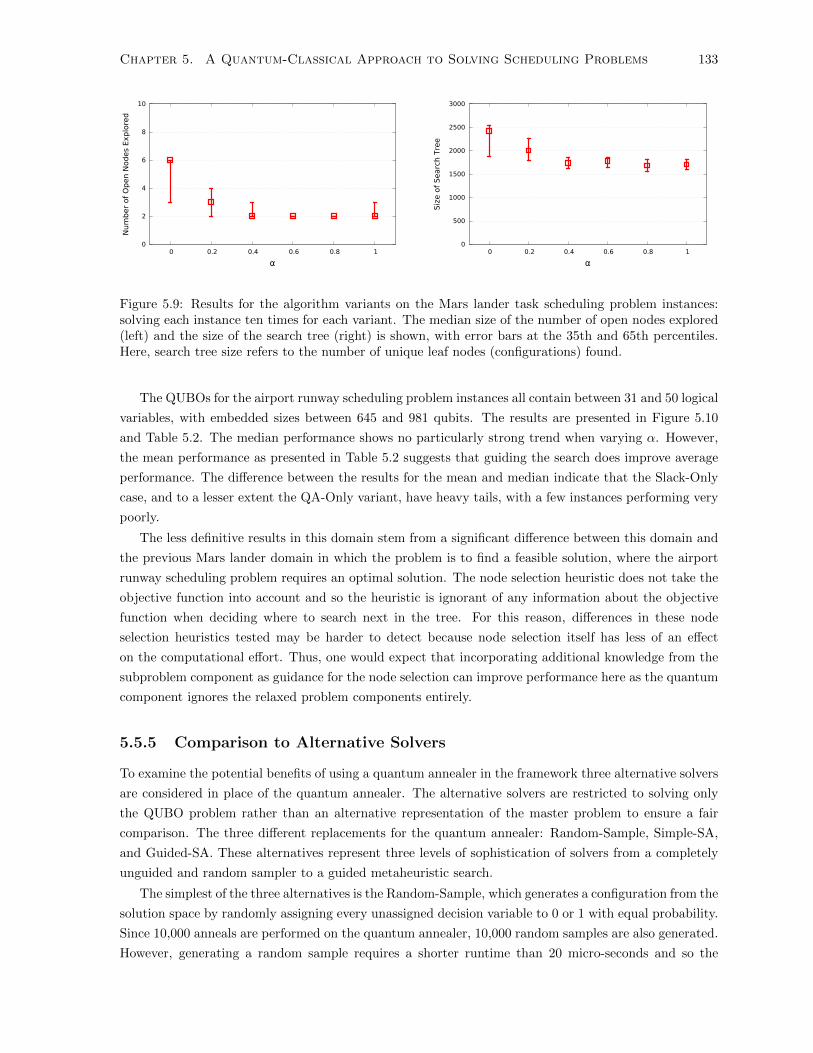
Chapter 5. A Quantum-Classical Approach to Solving Scheduling Problems 133
0
2
4
6
8
10
0 0.2 0.4 0.6 0.8 1
Num
ber
of
Op
en N
odes
Exp
lore
d
α
0
500
1000
1500
2000
2500
3000
0 0.2 0.4 0.6 0.8 1
Siz
e o
f S
earc
h T
ree
α
Figure 5.9: Results for the algorithm variants on the Mars lander task scheduling problem instances:solving each instance ten times for each variant. The median size of the number of open nodes explored(left) and the size of the search tree (right) is shown, with error bars at the 35th and 65th percentiles.Here, search tree size refers to the number of unique leaf nodes (configurations) found.
The QUBOs for the airport runway scheduling problem instances all contain between 31 and 50 logical
variables, with embedded sizes between 645 and 981 qubits. The results are presented in Figure 5.10
and Table 5.2. The median performance shows no particularly strong trend when varying α. However,
the mean performance as presented in Table 5.2 suggests that guiding the search does improve average
performance. The difference between the results for the mean and median indicate that the Slack-Only
case, and to a lesser extent the QA-Only variant, have heavy tails, with a few instances performing very
poorly.
The less definitive results in this domain stem from a significant difference between this domain and
the previous Mars lander domain in which the problem is to find a feasible solution, where the airport
runway scheduling problem requires an optimal solution. The node selection heuristic does not take the
objective function into account and so the heuristic is ignorant of any information about the objective
function when deciding where to search next in the tree. For this reason, differences in these node
selection heuristics tested may be harder to detect because node selection itself has less of an effect
on the computational effort. Thus, one would expect that incorporating additional knowledge from the
subproblem component as guidance for the node selection can improve performance here as the quantum
component ignores the relaxed problem components entirely.
5.5.5 Comparison to Alternative Solvers
To examine the potential benefits of using a quantum annealer in the framework three alternative solvers
are considered in place of the quantum annealer. The alternative solvers are restricted to solving only
the QUBO problem rather than an alternative representation of the master problem to ensure a fair
comparison. The three different replacements for the quantum annealer: Random-Sample, Simple-SA,
and Guided-SA. These alternatives represent three levels of sophistication of solvers from a completely
unguided and random sampler to a guided metaheuristic search.
The simplest of the three alternatives is the Random-Sample, which generates a configuration from the
solution space by randomly assigning every unassigned decision variable to 0 or 1 with equal probability.
Since 10,000 anneals are performed on the quantum annealer, 10,000 random samples are also generated.
However, generating a random sample requires a shorter runtime than 20 micro-seconds and so the

Chapter 5. A Quantum-Classical Approach to Solving Scheduling Problems 134
0
5
10
15
20
25
30
35
40
0 0.2 0.4 0.6 0.8 1
Num
ber
of
Op
en N
odes
Exp
lore
d
α
0
2000
4000
6000
8000
10000
12000
14000
16000
0 0.2 0.4 0.6 0.8 1
Siz
e o
f S
earc
h T
ree
α
Figure 5.10: Results for the algorithm variants on the airport runway scheduling problem instances:solving each instance ten times for each variant. The median size of the number of open nodes explored(left) and the size of the search tree (right) is shown, with error bars at the 35th and 65th percentiles.Here, search tree size refers to the number of unique leaf nodes (configurations) found.
Random-Sample approach is computationally cheaper.
The second alternative is Simple-SA, a basic simulated annealing approach [55, 143]. Simple-SA
starts with an initial state (assignment for x) and probabilistically decides whether to move to some
neighboring state x′ or stay in state x. Starting with a random configuration (generated in the same
was as Random-Sample), Simple-SA chooses a decision variable to flip; that is, if the variable is 0 (1),
it is changed to 1 (0). This new state is the neighboring state x′ and is always accepted if g(x′) < g(x).
If the current neighboring state is the best solution found so far, then this solution is recorded as the
current incumbent solution. When the neighboring state has an objective function worse than the
current state, x′ is accepted following a probability function P (g(x), g(x′), τ), where τ is a time-varying
parameter called the temperature. Like Kirkpatrick et al. [143], P (g(x), g(x′), τ) = e−(g(x′)−g(x))
τ . For
every neighboring state considered, a random value u = U [0, 1] is generated from a uniform distribution
and if u ≤ P (g(x), g(x′), τ), then x′ is accepted. The initial temperature is τ = 10 and is reduced
by 1% of the current value at each iteration. Each call to Simple-SA consists of 10,000 anneals for 20
micro-seconds each to match the quantum annealer, which results in 10,000 configurations that represent
the best solutions found during each anneal.
The final algorithm is Guided-SA, a more sophisticated simulated annealing approach. The premise
behind Guided-SA is that there is inherent structure to the scheduling problem that can be exploited.
Specifically, the domains of interest have a vertex, task, or aircraft, that must be assigned a single color
or time. Random-Sample and Simple-SA do not actively incorporate this constraint when generating
solutions. Therefore, to improve upon Simple-SA, the initial state and neighborhood is revised to
incorporate this structure within the simulated annealing heuristic. Instead of randomly sampling the
initial state, a vertex, task, or aircraft is chosen and one of the remaining values available from its domain
is selected at random. The neighborhood used is to randomly select one of the vertices, tasks, or aircraft
and change its color or time. All other components remain the same as in Simple-SA the same.
The Guided-SA approach can be considered a domain-dependent approach since it is actively making
use of specific problem structure to initialize and guide search. Although the underlying structure for all
three domains is the same (a job is assigned a single start-time), this structure is not always necessarily
present or obvious for all problems. A different structure might be used for another problem and
therefore, the Guided-SA approach must be customized to match the constraints of each problem. The

Chapter 5. A Quantum-Classical Approach to Solving Scheduling Problems 135
Algorithm 4 Simulated Annealing.
x = xox = xg∗ = g(x)τ = 10while runtime < 20 micro-seconds do
x′ = random neighbour(x)if g(x) > g(x′) or P (g(x), g(x′), τ) ≥ random(0, 1) then
x = x′
end ifτ = 0.99τif g(x) < g∗ theng∗ = g(x)x = x
end ifend while
three other approaches do not require such a level of customization. The QUBO may be customized
for the specific problem domain, but there is no search control embedded within the solver to guide
search for Random-Sample, Simple-SA or quantum annealing: these approaches are only given the cost
function of the QUBO to explore the solution space.
Algorithm 4 provides the pseudocode for the simulated annealing algorithm. Both Simple-SA and
Guided-SA follow this algorithm, but have different initial solutions xo and random neighbour(x) func-
tions.
The three alternative approaches are tested on the same set of instances previously used. Figure 5.11
shows the performance of all approaches using the best α value found from Sections 5.5.2 - 5.5.4. An
average of the median size of the search tree is presented. For all three domains, a similar pattern is seen
- Random-Sample is worst, Simple-SA is slightly better, and Guided-SA and Quantum are significantly
better than the other two, but roughly equivalent to each other except for in the Mars lander domain
where Quantum is better than Guided-SA.
5.6 Discussion
The results show that the quantum-classical hybrid framework can handle a variety of scheduling domains
with different objective functions and decomposition strategies. In this section, the benefits due to the
decomposition framework are discussed.
5.6.1 Decomposition: Benefits and Insights
The main benefit of the proposed decomposition is best seen when considering the current limitations of
the quantum hardware. Quantum annealing is still in an early stage of development and is not capable
of solving many scheduling problems. The purpose of the quantum-classical decomposition is to improve
upon the state of the quantum optimization literature.
A major issue with quantum hardware is the limited number of qubits. Since almost every scheduling
problem of interest for the automated scheduling community would require quantum annealers that are
orders of magnitude larger than current hardware, a pure quantum approach is impractical. The use of

Chapter 5. A Quantum-Classical Approach to Solving Scheduling Problems 136
(a) Graph Coloring
104
105
106
Random Simple SA Guided SA Quantum
Siz
e o
f S
earc
h T
ree
(b) Mars Lander Task Scheduling
103
104
105
106
Random Simple SA Guided SA Quantum
Siz
e o
f S
earc
h T
ree
(c) Airport Runway Scheduling
104
105
106
Random Simple SA Guided SA Quantum
Siz
e o
f S
earc
h T
ree
Figure 5.11: Results for the alternative algorithms on all problems. The median size of the search treeis shown, with error bars at the 35th and 65th percentiles. Here, search tree size refers to the numberof unique leaf nodes (configurations) found.
the decomposition allows for partial representation of a problem as the quantum component and solving
the remainder of the problem using classical methods. The Mars lander task scheduling problem shows
how the decomposition relaxes the problem by deferring the consideration of battery constraints to the
classical component after a schedule for the tasks is obtained.
Another aspect of quantum annealers that may be undesirable is that the process is incomplete.
That is, a pure quantum annealing approach cannot certify that a problem instance is infeasible for a
decision problem or that a feasible solution is optimal for an optimization problem. The graph coloring
problem illustrates the benefits of the decomposition best when a complete search is required. Given
that the graph coloring problem instances tested for this study are fully embeddable on the D-Wave 2X
chip, the decomposition is not necessary: a pure quantum annealing approach can find feasible colorings.
However, without the decomposition, it is possible that many anneals are performed but the quantum
annealer may still fail to find a feasible solution when one exists. The decomposition ensures that, given
enough time, the complete search space is explored.
The final major issue addressed by the quantum-classical decomposition is the 5-bit precision on the
D-Wave 2X system. This limitation restricts the expressivity of the QUBOs that can be solved and
is most apparent in constrained optimization problems, where constraints are represented as penalties
in the objective function. In order for the QUBO formulation to be correct, the penalties must be
sufficiently large to ensure that feasibility is not sacrificed for an improved objective value. In the

Chapter 5. A Quantum-Classical Approach to Solving Scheduling Problems 137
airport runway scheduling domain, the decomposition leaves the objective function evaluation for the
classical component so that the quantum annealer is strictly responsible for the feasibility problem.
Therefore, scaling the penalty to ensure feasibility is not required and the problem can be represented
with 5-bit precision.
The benefits from the perspective of improving quantum annealing are apparent, but it is also im-
portant to consider how quantum annealers can be beneficial within this decomposition framework. The
results in Section 5.5.5 provide some insights into potential advantages that can be further explored.
Specifically, Simple-SA and the quantum annealer can be considered to have access to the same infor-
mation. In both cases, no structural information is available; the solvers are given an objective function
over which to optimize. Yet the quantum annealer is significantly better than Simple-SA. In contrast,
the quantum annealer performs comparably, and even better than in one domain, in terms of search tree
size to Guided-SA, which makes use of structural knowledge by only searching solutions which assign
each node a single color or each task/aircraft a single time. This observation suggests that a quantum
annealing may be useful when the structure of a problem is not readily available.
It is suspected that this benefit is due to the process of quantum tunnelling that allows the state of a
qubit to change by tunnelling through a high energy barrier rather than increasing energy to exit a deep
valley [136]. In the scheduling problems studied, the energy landscape of the QUBO has many of these
deep valleys, because a single bit flip of a feasible solution will always lead to an increase in cost and an
immediate infeasibility. Simple-SA will always have to go over this energy barrier to explore different
solutions, whereas the quantum annealer does not. The quantum annealer might be a good choice as
a solver when expert system knowledge is not available, but further investigation is required to make
broader conclusions.
Moving away from the perspective of improving quantum annealing, it is possible to extend the
decomposition framework to purely classical solvers. Instead of using quantum annealing, it is possible
to use any heuristic solver as was done in Section 5.5.5. This framework would have the advantages of
metaheuristic solvers which will scale well to very large problems, while still maintaining a systematic
search due to the search tree.
5.7 Conclusion
A tree-search based quantum-classical framework is presented in which results from a quantum annealer
are used to prune and guide the search. The framework enables the use of a stochastic quantum-annealing
solver within a complete search framework. The results show the feasibility of integrating quantum and
classical computing and is the first study of its kind that proposes and fully implements such a hybrid
decomposition.
The approach is not limited to strictly quantum-classical algorithms. The framework can be applied
as a pure classical decomposition as seen in Section 5.5.5 and discussed in Section 5.6.1, allowing the
use of specialized heuristic solvers for large and difficult problems.
In general, one does not expect quantum annealers to be competitive in the near-term against classical
computing, with its decades-long headstart on research and development. Thus, one would expect that
a classical-classical decomposition would outperform a quantum-classical decomposition if a state-of-
the-art classical solver is used. The motivation in this work is to expand on the capabilities of the
current quantum annealers and to provide a framework in which the benefits of even mature quantum

Chapter 5. A Quantum-Classical Approach to Solving Scheduling Problems 138
annealing technology would be complemented by classical methods to obtain completeness and improve
performance.
A potential extension of this work is to incorporate additional classical heuristics into the tree search,
borrowing ideas from the extensive classical literature, such as variable ordering [30], conflict analysis and
cutting planes [1, 140], and discrepancy-based search [29, 115]. However, one may have to accommodate
the quantum annealer’s limitations to be able to fully implement these ideas effectively. For example,
one challenge is in keeping the resulting problems small enough that they can be run on current or
near-term quantum annealers. Additional variables would need to be added to the QUBO formulation
in order to incorporate constraints from cutting planes or no-good cuts. For this reason, it is interesting
to explore the design of such extensions within the context of quantum annealers.
Another extension is the application of improved pruning and selection algorithms within the pro-
posed framework to obtain better performance. Various inference methods for defining bounding func-
tions can be designed for particular problem domains. The tree search framework lends itself to tech-
niques found in constraint programming [244] and could benefit from the sophisticated inference algo-
rithms developed in that literature. Using a dynamic ordering to improve the effect of forward checking
is not currently performed, but is left as an area of improvement that can be implemented to enhance
performance.
There remains much to learn about quantum annealing and the interplay between classical and
quantum approaches. This work is an early step to provide insights into how to design and use special-
purpose quantum hardware in service of practical applications.
Chapter 6
Concluding Remarks
6.1 Summary
In this dissertation decomposition models are proposed to handle three different scheduling applications.
This study identified the complications that arise when trying to use a specific solving technique on a
scheduling problem and proposed decompositions that allowed the compensation of the shortcomings
of the chosen approaches through partitioning of a problem and using complementary techniques to
solve the components of the decomposition. The result was a scheduling approach that can be used
to solve the targeted scheduling applications whereas the pure, non-decomposed scheduling approaches
were inadequate: they were either unable to generate solutions within a reasonable amount of time
(Chapter 3) or they were not able to fully represent a problem (Chapters 4 and 5).
The dissertation took an engineering perspective to design decompositions for scheduling applications.
The approach was to identify limitations of a chosen technology in order to generate a partition of the
problem that can be represented and solved. In the case of Chapter 3, constraint programming (CP) is
used and the limitations of CP were its ineffectiveness for handling a complex multi-criteria objective
function and a large number of optional activities at the same time. The decomposition first considered
a problem with a simpler objective function and then used the resulting solution to restrict the decisions
regarding a subset of the optional activities in the second stage. The decomposition thereby allowed the
treatment of each of the complicating issues independently.
The decomposition in Chapter 4 was based on the fact that queueing theory and combinatorial
scheduling deal with different problem abstractions, dynamics and combinatorics, respectively. Each
of these approaches have tools to handle their respective problem abstractions. Although work exists
within each research area that does consider problem characteristics of the other, scheduling models with
dynamic job arrivals [190] for example, these studies are not the central focus of these research areas.
Thus, the techniques developed within each field are better tuned to represent and handle their core
problem abstractions. The proposed decomposition used techniques developed in queueing theory to first
account for the system dynamics and stochasticity. The solution to the dynamic system is then used
to guide combinatorial optimization by restricting the solution space to what are deemed to be “good”
solutions in the long-term. This combination of techniques from the two fields of research enabled a
more comprehensive representation of a data center scheduling environment and allowed for utilization
of the appropriate methodology to handle system dynamics and complex combinatorics.
139

Chapter 6. Concluding Remarks 140
Chapter 5 developed quantum annealing technology so that it can be used for scheduling problems.
The focus here was on identifying hardware limitations that restricted what can be embedded onto
existing quantum annealers as well as inherent limitations of quantum annealing itself, more specifically,
the fact that it is an incomplete, stochastic algorithm. A decomposition is introduced that embedded
the quantum annealer as a subroutine within an exhaustive tree search to compensate for the quantum
annealing limitations.
The three decompositions in this dissertation differed in the varying levels of integration between
solvers. The first decomposition (Chapter 3) can be considered the most straight-forward where a
problem is partitioned into two parts and solved using a single solver, CP. Through this type of a
decomposition, it was possible to significantly enhance the performance of a solver to the point where the
decomposition obtained good quality solutions to problem instances that a pure CP model could not find
even feasible solutions to. The second decomposition, in Chapter 4, made use of two solution techniques,
each developed in a different field of research. This decomposition has partitions that are fundamentally
different from a modelling and solving perspective, which allowed for the suitable handling of a problem
with features that are of core interest to queueing theory and combinatorial scheduling. Lastly, Chapter
5 not only combined solving techniques from two different fields of research, but also integrated two
different paradigms of computation into a cohesive algorithm. A hybrid classical computing and quantum
computing algorithm is created for solving combinatorial optimization problems.
6.2 Contributions
A number of contributions to the literature have been made on ad-hoc decompositions, the advancement
of understanding various solvers, and the state-of-the-art approaches to certain scheduling applications.
In this section, a summary of the contributions in each of the three main chapters of this dissertation
are presented.
Planning and Scheduling a Team of Mobile Robots in a Retirement Home
(Chapter 3)
1. A complex multi-robot human-robot interaction (HRI) problem was modelled with four different
solving technologies: AI Planning, Timeline-Based Planning and Scheduling, MIP, and CP. Di-
rect comparisons between these technologies are uncommon as each formalism contains its own
assumptions, restrictions, and solving techniques that affect how one can and should develop a
model.
2. A CP-based decomposition model was developed that outperformed all other tested approaches.
Results for a proposed CP model provided insights on the short-comings of the technology to handle
some aspects of the robot tasks scheduling system; the decomposition presented takes into account
these problematic aspects by ignoring one of the complicating aspects of the problem in the first
stage, and then reducing the search space of the problem in the second stage using the first-stage
solution. This decomposition allows the simplification of three other complicating aspects in order
to consistently obtain high quality solutions.
3. Alternative models in Planning Domain Definition Language (PDDL) for timed events and multi-
user actions were investigated. The principles and practice of taking a real problem and developing
Chapter 6. Concluding Remarks 141
a model are not often discussed and alternative models tend to not be explored in depth in the
planning community. This work contributes to the study of effective modeling.
4. One of the first applications of CP to a multi-robot planning and scheduling problem was intro-
duced. Automated planning is commonly proposed for handling decision making in robot systems.
The results showed that CP is a strong candidate with great potential to providing high quality
schedules.
Resource-Aware Scheduling for Heterogeneous Data Centers (Chapter 4)
1. A hybrid queueing theoretic and combinatorial optimization scheduling algorithm was proposed for
a data center. By decomposing the problem, it is possible to consider both the system dynamics and
complex combinatorics, providing a richer representation of the system than would be commonly
found in pure queueing theory or combinatorial scheduling approaches.
2. The allocation linear programming (LP) model [8] used for distributed computing [6] was extended
to a data center that has machines with multi-capacity resources. Such a system can have idle
resources because it cannot execute a set of jobs that simultaneously use all the resources of a
machine. Thus, the proposed model is more complex than the original allocation LP model as it is
important to account for these idle resources to accurately represent the behaviour of the system.
3. An empirical study of the scheduling algorithm was performed on both real workload trace data
and randomly generated data that showed that the decomposition performed orders of magnitude
better than existing techniques.
A Quantum-Classical Approach to Solving Scheduling Problems (Chapter 5)
1. A novel framework for quantum-classical hybrid approaches to combinatorial problems was pro-
posed. This framework is one of the first quantum-classical hybrid algorithms developed.
2. The first implementation of a quantum-classical decomposition that is actually run on quantum
hardware was performed. Until now, no other works have integrated a quantum computer and a
classical computer within a single hybrid framework.
3. The first use of quantum annealing in a complete search was introduced. Quantum annealing is
a stochastic solver and is not itself a complete technique. Through the use of the decomposition,
the quantum annealer is used as a sub-routine within a complete search framework.
6.3 Future Work
Future directions for research have been described in each of the content chapters of this dissertation.
Those directions focused on the specific application or decomposition developed. Here, the focus is on
more general directions coming from the work in this dissertation. Below, some potential decompositions
to explore are presented.

Chapter 6. Concluding Remarks 142
6.3.1 Planning and Scheduling Decompositions
In Chapter 3, a CP-based decomposition was proposed. The justification of using CP rather than AI
planning was that the empirical results showed the CP solver to be the most capable of four tested
solvers for generating high quality schedules. Specifically, by relaxing the problem to be solved, the CP
solver consistently found schedules with high user participation in Bingo games. The success of CP in
this study is application specific and it is not universally true that the use of CP within a decomposition
framework will be the correct choice. Therefore, alternative solvers should be examined for use in other
domains.
The initial intuition is that AI planning is better suited for decisions regarding whether a task should
be executed or not and CP is good at making sequencing decisions. The results in Chapter 3 did not
support this hypothesis, showing that the interaction of the solvers and the problem is much more
complicated than initially assumed. However, one of the reasons why CP could be used at all was
that the problem had a relatively natural scheduling representation: the number of instantiated actions
(tasks) required in the model was bounded and manageable. Yet, problem domains exist where tight
bounds on the number of times an operator is used is non-trivial. These domains result in an explosion
of the model size and are intractable for CP-based solvers. Therefore, there are cases where a planning
approach can be more suitable than a scheduling one.
Given that there are inherent strengths and weaknesses in planning and scheduling, a decomposition
that uses both planning and scheduling can be valuable. The benefit of the planning component can
be the expressiveness of the formalism to enable representation of planning problems that do not have
a natural scheduling representation. The scheduling component can then be responsible mostly for
resource assignment, task sequencing, and optimization.
One decomposition framework could be the integration of planning for the master problem and
scheduling for the sub-problem. Here, the planner might be useful for deciding on the actions to be
performed and the scheduler then sequences these actions. The benefit of such a decomposition is likely
to be found in problems where feasibility is difficult to obtain, but is not determined by the sequence of
actions: the sequence will mostly only affect the quality of a solution, so that feasibility would not be
compromised.
The work of Muise et al. [180] provides a good foundation for such a planning and scheduling hybrid.
They study the problem of generating a partial-order plan (POP), where some pairs within a set of
actions are ordered, from a given sequential plan, where there is a total ordering between every pair of
actions. The goal is to find a POP that has the fewest commitments (they use the fewest orderings as
a measure) in order to increase the flexibility of a plan to deal with uncertainties that arise during plan
execution. Alternative goals may be to generate robust POPs or stochastically optimal POPs for some
stochastic model of the environment. In systems with potentially more complex objective functions,
scheduling approaches can be favorable to the MaxSAT approach used by Muise et al.
In contrast, it is also possible to consider a hybrid decomposition that uses scheduling for the master
problem and planning for the subproblem. Logic-based Benders decomposition [127] is a framework
that can be used for such an integration. Typically in logic-based Benders decomposition, scheduling
problems are partitioned into a resource assignment master problem that optimizes some function and
a subproblem that is a sequencing problem which checks feasibility [85, 127, 235]. This partitioning
scheme works well because deciding on the assignment and the sequencing are difficult together, but
significantly easier in isolation. Thus, a relaxation of the sequencing decisions is made in the master

Chapter 6. Concluding Remarks 143
problem, and a sequence is then obtained for each resource in the subproblem.
Incorporating the planner as a subproblem solver allows for one to work with problems that may
not have a natural scheduling representation, but have ones more suited to planning. The complicating
components that are more amenable to planning can be relaxed in the master problem and then solved
later. Burt et al. [51] developed such a decomposition. However, they did not implement logic-based
Benders decomposition. Rather, a two-stage decomposition is used, which is equivalent to a single
iteration of the logic-based Benders decomposition. A complete approach that allows for bi-directional
communication between the master problem and subproblem can be more generally applicable than the
uni-directional approach of Burt et al.
6.3.2 Queueing and Scheduling Decompositions
Another direction is to explore more general queueing theory and scheduling frameworks that can be
applied to a broad range of dynamic scheduling problems. In some previous work, similar queueing-
scheduling hybrids to the one proposed in Chapter 4 were developed [233, 237]. These models share the
same structure of using an allocation linear program (LP) developed in the queueing theory literature
to guide lower-level combinatorial scheduling decisions. This framework can be used successfully for
dynamic scheduling problems with a resource assignment component. The idea is to use fluid represen-
tations (that is, the allocation LP) to provide recommendations for the assignment decisions. Then, it
is possible to create schedules based on online realizations of job arrivals that use the recommendations
from the allocation LP to ensure that the long-term performance of the system does not suffer. Creating
a general framework for dynamic scheduling using this decomposition scheme is a promising research
direction.
Another possible decomposition is to represent parts of a system as queueing networks and then
use combinatorial optimization to make decisions regarding how to use them. The bin generation and
machine assignment LP of Chapter 4 is an example of how one might use this decomposition. The
bins represent possible combinations of jobs on a machine and were used to represent the long-term
assignment of jobs to the machine. However, the bins made use of the expected resource consumption of
jobs, which is not an accurate model for representing actual resource utilization of a machine; the amount
of resources requested by a job may vary from expectation and the exact mix of jobs can differ from
the mix defined by a bin. For a more accurate model, one can treat each machine as a single machine
queueing system with different job classes, where the arrival rate of jobs depends on the mix of jobs as
defined by the bin. This model provides a better description of the actual behavior of a machine than
the bins as defined in Chapter 4. An optimization model might then be used at a high-level to consider
the overall system and solve a combinatorial problem regarding the many smaller queueing networks to
decide which bins (queues) each machine should emulate. If the queueing network is simple, queueing
models can be utilized to understand the long-term performance of the network. In the data center
scheduling application, the queueing system defined by a bin was not simple enough that one could
easily obtain an accurate model due to the resource usage property, so instead a basic representation
using the mean values of resource usage was used.
The optimization over these smaller queueing networks can either be done by first generating all
relevant queuing networks and then determining which networks to use (similar to the second stage of
LoTES in Chapter 4), or optimization can be done without knowledge of the queueing networks, and
the solutions from the combinatorial problem then describe the queueing network to be solved in a

Chapter 6. Concluding Remarks 144
subsequent stage. The latter scheme deviates further from the decomposition found in this dissertation,
but is structurally similar to logic-based Benders decomposition, where the subproblems are the resulting
queueing networks that are used to check consistency of the master problem solution.
For example, consider a system where there are multiple job classes defined by the set K and multiple
heterogeneous machines with controllable speed defined by the set M . The amount of work required
for a job j belonging to class k ∈ K on machine m ∈ M is denoted as wjm and is independent and
identically distributed with mean Wkm. The processing time of job j on machine m depends on the
speed setting of a machine. Assume that a speed multiplier can be set on a machine, sm, such that the
processing time of a job j on machine m is djm =wjmsm
. The speed of these machines are equal to 1
by default, but can be increased by incurring a cost defined by the function c(sm). If a constraint is
enforced on the quality of service of this system such that the expected waiting time of jobs assigned to
any single machine is less than some threshold Ω, then a solution to this problem is an assignment of
the proportion of jobs from a job class to machines, pkm, and the speed of each machine, sm, such that
the waiting time constraint is met and the total cost,∑m∈M c(sm), is minimized. The master problem
could determine a minimum cost solution for the job assignment, pkm, and speed of each machine, sm,
while ignoring the quality of service constraint. The subproblem would use the job assignment and the
machine speed as an input and would be a descriptive queueing model of the long-run performance of
the machine to be compared against Ω to enforce quality of service. When a machine is not able to
meet its quality of service requirements, a Benders cut is sent back to the master problem to remove the
current solution such that either the workload is lessened or the speed of the machine is increased.
6.3.3 Sampling-Based Metaheuristics for Tree Search
The tree search algorithm presented in Chapter 5 illustrated how one can use a heuristic sampling ap-
proach to populate a search tree. A natural extension of this procedure is to use classical computing
metaheuristics rather than quantum annealing, which one would expect to result in improved perfor-
mance since the quantum annealer is not yet competitive with classical computers on a vast majority of
combinatorial optimization problems. Given that the classical computing algorithms do not share the
same limitations as the quantum annealer, there can be many improvements to the algorithm to allow
for a richer search procedure. For example, one can now more easily update the problem to be solved by
the metaheuristic (recall that updating the problem solved by the quantum annealer to add constraints
and/or variables requires a new embedding) to include cuts or search guidance based on inferences made
in other parts of the tree. With a classical computer, a more refined algorithm can be made.
The sampling based search can also be considered in other frameworks. For example, incorporating
ideas from the tree search algorithm into CP search might help to improve the performance of CP solvers.
A sampling-based metaheuristic can be used at a search node to rapidly populate the tree below the
node. The idea is that the heuristic solver should be chosen and designed so that it has the potential for
finding a solution quickly. A large population of solutions are returned and one or more feasible solutions
may be in the population of solutions. For constraint satisfaction problems, finding a feasible solution
is sufficient condition to terminate search. In the case of constraint optimization problems, increasing
the likelihood of finding high quality solutions can help prune the search tree. One can also explore a
large variety of deeper nodes, expanding the frontier defined by the open nodes considered for expansion.
Such an integration allows for one to benefit from the structural reasoning and speed of a metaheuristic,
while also maintaining the strong inference algorithms and the methodological search procedure of CP.

Chapter 6. Concluding Remarks 145
Similar techniques are are used in MIP solvers as primal heuristics [39], which aim to generate solutions
with good objective function values in short running times to provide a good feasible solution for the
branch-and-cut algorithm. The difference between the proposed approach and primal heuristics is in
the use of a population of samples that not only is useful for obtaining feasible solutions, but also for
populating the search tree and can be used to explore infeasible regions, to help prune the search tree,
as well.
6.3.4 Quantum Annealing for Monte-Carlo Tree Search
Monte Carlo tree search (MCTS) [68] is a popular approach to solving sequential decision making
problems, particularly games and planning problems [50]. The central idea behind MCTS is to perform
a Monte Carlo evaluation at nodes in the search tree to estimate the value of a state using several random
simulations. The algorithm progressively builds a partial tree, choosing nodes to expand in a best-first
order according to the results of the Monte Carlo evaluations. Once a node has been evaluated, the
result is used to update all ancestor nodes to obtain a more accurate assessment on their values for use
in subsequent steps.
Conceptually, MCTS is similar to the tree search proposed in Chapter 5, so a natural extension is
to incorporate the quantum annealer into MCTS. Rather than use a Monte Carlo simulation to obtain
random samples, the quantum annealer can be used. The main difference between MCTS and the tree
search is how the search tree is built. Recall that each sample from the quantum annealer is used to
populate a trajectory from the current search node to a leaf node in the proposed algorithm. In contrast,
a Monte Carlo sample (also called a rollout) is used to assign a value to the search node. Although a
trajectory from the current search node to a leaf node is also represented by a rollout, this sequence
of decisions (representing a sequence of nodes in the search tree) is not added to the tree. Rather, the
rollout is only used to evaluate the current state of a node.
Unlike MCTS approaches that only generate a single sample at a time to evaluate a node, the use of
quantum annealing dictates that many samples be produced any time one must evaluate a node. With
a large sample size, the valuation of a state is expected to be more accurate since more information can
be gathered immediately rather than delaying until the particular branch is expanded multiple times.
However, a trade-off is that more time is spent at each node.
Based on the results observed when comparing quantum annealing to variations of simulated anneal-
ing with and without structural guidance in Chapter 5, it is conjectured that quantum annealing might
be better applied to solving problems where minimal search control built into the solver is required.
This characteristic can be seen to be desirable for an MCTS-based system that is tasked to adapt to
and play different games. Rather than having to understand complex problem structures of games and
implement heuristics and policies specific to a game, quantum annealing is promising as a minimal con-
trol approach. The importance of having a good policy within an MCTS is made apparent in recent
successes of Google DeepMind’s AlphaGo [220] program for playing the game Go, where deep neural
networks are used to obtain value networks to evaluate board positions and policy networks to select
moves in a MCTS framework. The premise of using quantum annealing is that it might take the place
of the policy network.
The only major hurdle of using quantum annealing for playing games in an MCTS framework is the
requirement of a quadratic unconstrained binary optimization formulation that accurately captures the
reward function of a sequence of decisions in a game. However, even without representation of a reward

Chapter 6. Concluding Remarks 146
function, one can still use quantum annealing to sample feasible sequences of decisions, but the benefits
of choosing better actions can be lost as the samples will be more randomly distributed over the feasible
solution space instead of focused towards higher quality solutions. These less informed models may still
work well, as there have been numerous successful Go programs based on MCTS without the value and
policy networks of AlphaGo [50].
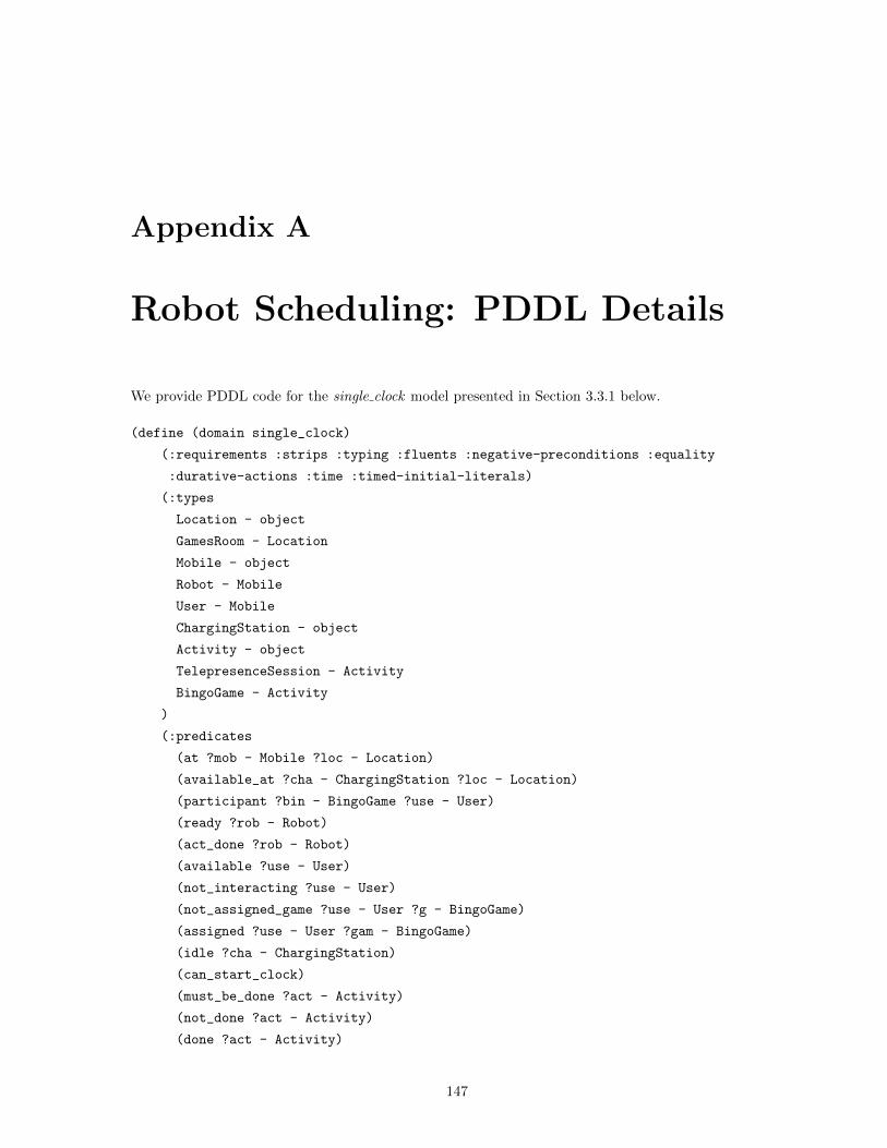
Appendix A
Robot Scheduling: PDDL Details
We provide PDDL code for the single clock model presented in Section 3.3.1 below.
(define (domain single_clock)
(:requirements :strips :typing :fluents :negative-preconditions :equality
:durative-actions :time :timed-initial-literals)
(:types
Location - object
GamesRoom - Location
Mobile - object
Robot - Mobile
User - Mobile
ChargingStation - object
Activity - object
TelepresenceSession - Activity
BingoGame - Activity
)
(:predicates
(at ?mob - Mobile ?loc - Location)
(available_at ?cha - ChargingStation ?loc - Location)
(participant ?bin - BingoGame ?use - User)
(ready ?rob - Robot)
(act_done ?rob - Robot)
(available ?use - User)
(not_interacting ?use - User)
(not_assigned_game ?use - User ?g - BingoGame)
(assigned ?use - User ?gam - BingoGame)
(idle ?cha - ChargingStation)
(can_start_clock)
(must_be_done ?act - Activity)
(not_done ?act - Activity)
(done ?act - Activity)
147

Appendix A. Robot Scheduling: PDDL Details 148
(free ?gam - GamesRoom)
(playing ?rob - Robot ?bin - BingoGame)
(room ?use - User ?loc - Location)
(local_user ?tel - TelepresenceSession ?use - User)
(game_location ?bin - BingoGame ?gam - GamesRoom)
)
(:functions
(bl ?rob - Robot)
(bl_min ?rob - Robot)
(bl_max ?rob - Robot)
(v ?rob - Robot)
(cr_move ?rob - Robot)
(cr_telep ?rob - Robot)
(cr_remind ?rob - Robot)
(cr_bingo ?rob - Robot)
(rr ?rob - Robot)
(att_min ?use - User)
(att_max ?use - User)
(att_num ?use - User)
(id ?use - User)
(distance ?l1 - Location ?l2 - Location)
(distance_to_station ?loc - Location ?cs - ChargingStation)
(games_attendees)
(current_time)
(delivery_time_limit_max)
(delivery_time_limit_min)
(total_delivery_time)
(total_battery_usage)
(total_number_users)
(games_skipped)
(dur_remind ?bin - BingoGame)
(p_min ?bin - BingoGame)
(p_max ?bin - BingoGame)
(p_num ?bin - BingoGame)
(delivery_time ?bin - BingoGame ?u - User)
(p_cur ?bin - BingoGame)
(dur ?act - Activity)
(action_duration ?act - Activity))
(:process clock_ticker
:parameters ()
:precondition

Appendix A. Robot Scheduling: PDDL Details 149
(can_start_clock)
:effect
(increase (current_time) (* #t 1.0)))
(:durative-action move
:parameters (?self - Robot ?from - Location ?to - Location ?cs - ChargingStation)
:duration (= ?duration (/ (distance ?from ?to) (v ?self)))
:condition
(and
(at start (ready ?self))
(at start (at ?self ?from))
(at start (not (= ?from ?to)))
(at start (act_done ?self))
(at start (> (bl ?self) (+ (* (/ (+ (distance ?from ?to)
(distance_to_station ?to ?cs)) (v ?self)) (cr_move ?self))
(bl_min ?self))))
)
:effect
(and
(at start (not (at ?self ?from)))
(at start (not (ready ?self)))
(at end (at ?self ?to))
(at end (ready ?self))
(at start (not (act_done ?self)))
(at start (decrease (bl ?self) (* (/ (distance ?from ?to) (v ?self))
(cr_move ?self))))
(at start (increase (total_battery_usage) (* (/ (distance ?from ?to)
(v ?self)) (cr_move ?self))))))
(:durative-action do_telepresence
:parameters (?self - Robot ?s - TelepresenceSession ?u - User ?loc - Location
?cs - ChargingStation)
:duration (= ?duration (dur ?s))
:condition
(and
(over all (at ?self ?loc))
(over all (at ?u ?loc))
(over all (available ?u))
(over all (must_be_done ?s))
(at start (ready ?self))
(at start (at ?self ?loc))
(at start (at ?u ?loc))
(at start (available ?u))

Appendix A. Robot Scheduling: PDDL Details 150
(at start (not_interacting ?u))
(at start (local_user ?s ?u))
(at start (must_be_done ?s))
(at start (room ?u ?loc))
(at start (not_done ?s))
(at start (>= (bl ?self) (+ (+ (* (dur ?s) (cr_telep ?self))
(* (/ (distance_to_station ?loc ?cs) (v ?self)) (cr_move ?self)))
(bl_min ?self))))
)
:effect
(and
(at start (not (ready ?self)))
(at start (not (not_interacting ?u)))
(at end (ready ?self))
(at end (done ?s))
(at end (not_interacting ?u))
(at start (not (not_done ?s)))
(at end (act_done ?self))
(at start (decrease (bl ?self) (* (dur ?s) (cr_telep ?self))))
(at start (increase (total_battery_usage) (* (dur ?s) (cr_telep ?self))))))
(:durative-action recharge
:parameters (?self - Robot ?loc - Location ?cs - ChargingStation)
:duration (= ?duration (/ (- (bl_max ?self) (bl ?self)) (rr ?self)))
:condition
(and
(at start (ready ?self))
(at start (at ?self ?loc))
(at start (available_at ?cs ?loc))
(at start (idle ?cs))
(over all (at ?self ?loc))
(at start (< (bl ?self) (bl_max ?self)))
)
:effect
(and
(at start (not (idle ?cs)))
(at start (not (ready ?self)))
(at end (idle ?cs))
(at end (ready ?self))
(at start (assign (bl ?self) (bl_max ?self)))
(at end (act_done ?self))))
(:durative-action remind

Appendix A. Robot Scheduling: PDDL Details 151
:parameters (?self - Robot ?u - User ?g - BingoGame ?loc - Location
?cs - ChargingStation)
:duration (= ?duration (dur_remind ?g))
:condition
(and
(over all (at ?self ?loc))
(over all (at ?u ?loc))
(over all (available ?u))
(at start (ready ?self))
(at start (at ?self ?loc))
(at start (at ?u ?loc))
(at start (available ?u))
(at start (not_interacting ?u))
(at start (not_done ?g))
(at start (< (p_num ?g) (p_max ?g)))
(at start (not_assigned_game ?u ?g))
(at start (< (att_num ?u) (att_max ?u)))
(at start (>= (bl ?self) (+ (+ (* (dur_remind ?g)
(cr_remind ?self)) (* (distance_to_station ?loc ?cs)
(cr_move ?self))) (bl_min ?self))))
)
:effect
(and
(at start (not (ready ?self)))
(at start (not (not_interacting ?u)))
(at end (ready ?self))
(at end (not_interacting ?u))
(at start (increase (p_num ?g) 1))
(at start (participant ?g ?u))
(at start (not (not_assigned_game ?u ?g)))
(at start (increase (att_num ?u) 1))
(at end (act_done ?self))
(at start (decrease (bl ?self) (* (dur_remind ?g)
(cr_remind ?self))))
(at start (assign (delivery_time ?g ?u) (current_time)))
(at start (increase (total_battery_usage)
(* (dur_remind ?g) (cr_remind ?self))))))
(:action skip_bingo
:parameters (?g - BingoGame)
:precondition

Appendix A. Robot Scheduling: PDDL Details 152
(and
(must_be_done ?g)
(not_done ?g)
(= (p_num ?g) 0)
)
:effect
(and
(not (not_done ?g))
(done ?g)
(increase (games_skipped) 1)))
(:durative-action play_Bingo
:parameters (?self - Robot ?g - BingoGame ?loc - GamesRoom
?cs - ChargingStation)
:duration (= ?duration (dur ?g))
:condition
(and
(at start (at ?self ?loc))
(over all (at ?self ?loc))
(at start (ready ?self))
(at start (must_be_done_during ?g))
(over all (must_be_done_during ?g))
(at start (game_location ?g ?loc))
(at start (not_done ?g))
(at start (<= (p_num ?g) (p_max ?g)))
(at start (> (p_num ?g) (- (p_min ?g) 1)))
(at end (= (p_cur ?g) (p_num ?g)))
(at start (>= (bl ?self) (+ (+ (* (dur ?g) (cr_Bingo ?self))
(* (distance_to_station ?loc ?cs) (cr_move ?self)))
(bl_min ?self))))
(at start (free ?loc)))
:effect
(and
(at start (not (ready ?self)))
(at end (ready ?self))
(at end (done ?g))
(at start (not (not_done ?g)))
(at start (playing ?self ?g))
(at end (not (playing ?self ?g)))
(at end (act_done ?self))
(at start (decrease (bl ?self) (* (dur ?g) (cr_Bingo ?self))))
(at start (increase (total_battery_usage) (* (dur ?g)
(cr_Bingo ?self))))

Appendix A. Robot Scheduling: PDDL Details 153
(at start (increase (games_attendees) (p_num ?g)))
(at start (not (free ?loc)))
(at end (free ?loc))))
(:durative-action interact
:parameters (?self - Robot ?g - BingoGame ?u - User)
:duration (= ?duration (- (dur ?g) 1))
:condition
(and
(at start (playing ?self ?g))
(over all (playing ?self ?g))
(at start (available ?u))
(over all (available ?u))
(at start (not_interacting ?u))
(at start (participant ?g ?u))
(at start (>= (delivery_time_limit_max)
(- (current_time) (delivery_time ?g ?u))))
(at start (<= (delivery_time_limit_min)
(- (current_time) (delivery_time ?g ?u)))))
:effect
(and
(at start (increase (p_cur ?g) 1))
(at start (not (not_interacting ?u)))
(at end (not_interacting ?u))
(at start (increase (total_delivery_time)
(- (current_time) (delivery_time ?g ?u))))))
)
Below, the play Bingo3 operator is presented. This operator is used for the min add and set all
models. For the min add models, the operator is used as is. For the set all models, the play Bingo3
operator is expanded to include multiple play BingoX operators, one for each possible value of X (the
number of users that can participate in a Bingo game). In the case of set all, one must update the
operator to have the correct number of users, rather than just three users as presented here.
(:durative-action play_Bingo3
:parameters (?self - Robot ?g - BingoGame ?loc - GamesRoom ?u1 - User
?u2 - User ?u3 - User ?cs - ChargingStation)
:duration (= ?duration (dur ?g))
:condition
(and
(at start (at ?self ?loc))
(over all (at ?self ?loc))
(at start (ready ?self))
(at start (must_be_done_during ?g))
(over all (must_be_done_during ?g))

Appendix A. Robot Scheduling: PDDL Details 154
(at start (game_location ?g ?loc))
(at start (not_done ?g))
(at start (<= (p_num ?g) (p_max ?g)))
(at start (> (p_num ?g) (- (p_min ?g) 1)))
(at end (= (p_cur ?g) (p_num ?g)))
(at start (>= (bl ?self) (+ (+ (* (dur ?g) (cr_Bingo ?self))
(* (distance_to_station ?loc ?cs) (cr_move ?self)))
(bl_min ?self))))
(at start (free ?loc)))
(at start (available ?u1))
(over all (available ?u1))
(at start (not_interacting ?u1))
(at start (participant ?g ?u1))
(at start (>= (delivery_time_limit_max) (- (current_time)
(delivery_time ?g ?u1))))
(at start (<= (delivery_time_limit_min) (- (current_time)
(delivery_time ?g ?u1))))
(at start (available ?u2))
(over all (available ?u2))
(at start (not_interacting ?u2))
(at start (participant ?g ?u2))
(at start (>= (delivery_time_limit_max) (- (current_time)
(delivery_time ?g ?u2))))
(at start (<= (delivery_time_limit_min) (- (current_time)
(delivery_time ?g ?u2))))
(at start (available ?u3))
(over all (available ?u3))
(at start (not_interacting ?u3))
(at start (participant ?g ?u3))
(at start (>= (delivery_time_limit_max) (- (current_time)
(delivery_time ?g ?u3))))
(at start (<= (delivery_time_limit_min) (- (current_time)
(delivery_time ?g ?u3))))
(at start (not (= ?u1 ?u2)))
(at start (not (= ?u1 ?u3)))
(at start (not (= ?u2 ?u3)))
(at start (< (id ?u1) (id ?u2)))
(at start (< (id ?u2) (id ?u3)))
(at start (assigned ?u1 ?g))
(at start (assigned ?u2 ?g))
(at start (assigned ?u3 ?g))
:effect
(and

Appendix A. Robot Scheduling: PDDL Details 155
(at start (not (ready ?self)))
(at end (ready ?self))
(at end (done ?g))
(at start (not (not_done ?g)))
(at start (playing ?self ?g))
(at end (not (playing ?self ?g)))
(at end (act_done ?self))
(at start (decrease (bl ?self) (* (dur ?g) (cr_Bingo ?self))))
(at start (increase (total_battery_usage) (* (dur ?g)
(cr_Bingo ?self))))
(at start (increase (games_attendees) 3))
(at start (not (free ?loc)))
(at end (free ?loc)))
(at start (increase (p_cur ?g) 3))
(at start (not (not_interacting ?u1)))
(at end (not_interacting ?u1))
(at start (increase (total_delivery_time)
(+ (- (current_time) (delivery_time ?g ?u3))
(+ (- (current_time) (delivery_time ?g ?u2))
(- (current_time) (delivery_time ?g ?u1))))))
(at start (not (not_interacting ?u2)))
(at end (not_interacting ?u2))
(at start (not (not_interacting ?u3)))
(at end (not_interacting ?u3))
(at start (increase (p_num ?g) 3)))
Below, the two operators Bingo overall and setup Bingo are presented. These operators are necessary
for the envelope models.
(:durative-action Bingo_overall
:parameters (?g - BingoGame)
:duration (= ?duration (+ (dur ?g) (delivery_time_limit_max))
:condition
(and
(at start (not_done ?g))
(at start (not_Bingo_actions_ready ?g)))
:effect
(and
(at start (not (not_Bingo_actions_ready ?g)))
(at start (Bingo_actions_ready ?g))
(at end (not (Bingo_actions_ready ?g)))
(at start (remind_enable ?g))))
(:durative-action setup_Bingo
:parameters (?g - BingoGame)

Appendix A. Robot Scheduling: PDDL Details 156
:duration (= ?duration (delivery_time_limit_min))
:condition
(and
(at start (Bingo_actions_ready ?g))
(over all (Bingo_actions_ready ?g))
(at start (remind_enable ?g))
(at start (not_done ?g)))
:effect
(and
(at start (not (remind_enable ?g)))
(at end (Bingo_game_ready ?g))))

Appendix B
Robot Scheduling: NDDL Details
We provide NDDL code for the Move and PlayBingo actions. The code illustrates the requirements and
effects of the actions and how these actions interact with the state of the system. Since no full NDDL
models were created due to limitations of the solver, we only provide these definitions as an indication
of the modeling.
class Location
string name;
class Path
string name;
Location from;
Location to;
float distance;
class ChargingStation
Location charging_station;
ChargingStationUsage charging_station_usage;
class ChargingStationUsage extends Reusable
string profileType;
string detectorType;
ChargingStationUsage()
super (1, 0);
profileType = "GroundedProfile";
detectorType = "GroundedFVDetector";
class TelepresenceSession
string name;
TelepresenceSessionState status;
User localuser;
157

Appendix B. Robot Scheduling: NDDL Details 158
Location location;
int dur;
class TelepresenceSessionState extends Timeline
predicate MustBeDone
predicate InProgress
predicate Done
class BingoGame
string name;
BingoGameState status;
Location location;
int dur;
int players;
class BingoGameState extends Timeline
predicate MustBeDone
predicate InProgress
predicate Done
class User
string name;
int deliveryTime;
UserState state;
UserAvailability availability;
UserGameAssignment assignment;
class UserState extends Timeline
predicate At Location location;
predicate Interacting Robot robot;
predicate Playing Robot robot; BingoGame game;
predicate BeingReminded Robot robot;
class UserAvailability extends Timeline
predicate Available
predicate Busy
class UserGameAssignment extends Timeline
predicate NotAssigned
predicate BeingAssigned
predicate Assigned BingoGame game;
class Robot
string name;
RobotState status;
Battery battery;

Appendix B. Robot Scheduling: NDDL Details 159
float speed;
int cr_move;
int recharge_rate;
int cr_telep;
int cr_bingo;
int cr_reminder;
// Actions
action Move
Path path;
Location destination;
action RechargeBattery
ChargingStation station;
action DoTelepresence
TelepresenceSession session;
User user;
action PlayBingo
BingoGame game;
User user;
User user2;
User user3;
GameRoomUsage gameRoom;
neq(user,user2);
neq(user,user3);
neq(user2,user3);
action Remind
BingoGame game;
User user;
class RobotState extends Timeline
predicate FreeAt Location location;
predicate Moving Location destination;
predicate Charging Location location;
predicate DoingTelepresence TelepresenceSession session; User user;
predicate Reminding BingoGame game; User user;
predicate PlayingGame BingoGame game;
class Battery extends Reservoir
string profileType;
string detectorType;

Appendix B. Robot Scheduling: NDDL Details 160
Battery(int _ini, int _min, int _max)
super(_ini, _min, _max);
profileType="GroundedProfile";
detectorType = "GroundedFVDetector";
Robot::Move
met_by(condition object.status.FreeAt _from);
eq(_from.location,path.from);
eq(destination, path.to);
meets(effect object.status.FreeAt _to);
eq(_to.location, destination);
neq(_from.location, destination);
eq(effect object.status.Moving _moving);
eq(_moving.destination, destination);
float dura, dist, vel, energy_use, c_move;
dist == path.distance;
vel == object.speed;
c_move == object.cr_move;
dist == dura * vel;
energy_use == dura * c_move;
starts(effect object.battery.consume cons);
eq(cons.quantity, energy_use);
eq(dura,duration);
Robot::PlayBingo
met_by(condition object.status.FreeAt _robotFreeAtStart);
met_by(condition game.status.MustBeDone _gameStart);
eq(game.location,_robotFreeAtStart.location);
contained_by(condition user1.availability.Available _user1Available);
contained_by(condition user2.availability.Available _user2Available);
contained_by(condition user3.availability.Available _user3Available);
met_by(condition user1.assignment.Assigned _user1Assigned);
met_by(condition user2.assignment.Assigned _user2Assigned);
met_by(condition user3.assignment.Assigned _user3Assigned);
eq(_user1Assigned.game, game);
eq(_user2Assigned.game, game);
eq(_user3Assigned.game, game);
eq(effect object.status.PlayingGame _interactingRobot);
eq(_interactingRobot.game, game);
meets(effect object.status.FreeAt _robotFreeAtEnd);
eq(_robotFreeAtStart.location,_robotFreeAtEnd.location);
eq(effect user1.state.Interacting _interactingUser1);
eq(_interactingUser1.robot, object);

Appendix B. Robot Scheduling: NDDL Details 161
eq(effect user2.state.Interacting _interactingUser2);
eq(_interactingUser2.robot, object);
eq(effect user3.state.Interacting _interactingUser3);
eq(_interactingUser3.robot, object);
meets(effect user1.state.At _user1AtEnd);
eq(_robotFreeAtStart.location,_user1AtEnd.location);
meets(effect user2.state.At _user2AtEnd);
eq(_robotFreeAtStart.location,_user2AtEnd.location);
meets(effect user3.state.At _user3AtEnd);
eq(_robotFreeAtStart.location,_user3AtEnd.location);
equals(effect game.status.InProgress _gameProgress);
meets(effect game.status.Done _gameDone);
eq(_gameDone.end, Horizon);
eq(GameRoomUsage.uses use_room);
int user1Delivery, user2Delivery, user2Delivery;
user1Delivery == _interactingRobot.start - user1.deliveryTime;
user2Delivery == _interactingRobot.start - user2.deliveryTime;
user3Delivery == _interactingRobot.start - user3.deliveryTime;
user1Delivery >= 15;
user1Delivery <= 120;
user2Delivery >= 15;
user2Delivery <= 120;
user3Delivery >= 15;
user3Delivery <= 120;
eq(game.dur, use_room.duration);
eq (use_room.quantity, 1);
int _cr_bingo, dura, energy_use_bingo;
_cr_bingo == object.cr_bingo;
dura == game.dur;
energy_use_bingo == dura * _cr_bingo;
starts(effect object.battery.consume cons);
eq(cons.quantity, energy_use_bingo);
eq(game.dur, duration);

Appendix C
Robot Scheduling: Detailed PDDL
Results
Detailed results for all the PDDL planning models tested on each of the problem variants are presented
here. The first and last feasible solutions found within a one-hour time limit is recorded.
162

Appendix C. Robot Scheduling: Detailed PDDL Results 163
Table C.1: Performance of PDDL planning on all tested problem modifications for the single-clock model.A (-) indicates that no solution was found.
Problem Scenario Runtime (s) Participants Objective Valuefirst last first last first last
1 0.04 786.12 0 3 5,506.13 2,070.752 0.18 0.88 0 0 11,019.38 11,016.66
BRPOF 3 0.84 9.38 0 0 16,530.31 16,525.734 2.18 23.84 0 0 22,044.46 22,043.115 7.24 89.46 0 0 27,557.30 27,554.54
1 0.02 345.02 0 3 5,500.00 2,051.232 0.12 306.00 0 4 11,000.00 7,208.00
-RPOF 3 0.34 0.34 0 0 16,500.00 16,500.004 0.92 0.92 0 0 22,000.00 22,000.005 1.94 1.94 0 0 27,500.00 27,500.00
1 0.04 168.42 0 3 5,506.13 2,070.412 0.18 0.78 0 0 11,019.38 11,016.66
B-POF 3 0.74 7.24 0 0 16,530.31 16,525.734 1.90 16.62 0 0 22,044.46 22,043.115 6.10 66.33 0 0 27,557.30 27,554.54
1 0.04 761.99 0 0 5,508.49 5,506.782 0.18 0.88 0 0 11,019.38 11,016.66
BR-OF 3 0.84 9.02 0 0 16,530.31 16,525.734 2.16 22.88 0 0 22,044.46 22,043.115 7.16 92.06 0 0 27,557.30 27,554.54
1 - - - - - -2 - - - - - -
BRP-F 3 - - - - - -4 - - - - - -5 - - - - - -
1 0.06 75.94 0 3 5,612.46 2,761.642 0.18 0.18 0 0 11,019.38 11,019.38
BRPO- 3 0.82 0.82 0 0 16,530.31 16,530.314 2.18 2.18 0 0 22,044.46 22,044.465 7.04 7.04 0 0 27,557.30 27,557.30
1 0.10 163.72 4 4 1,013.33 1,013.222 4.38 391.42 8 8 2,526.20 2,526.09
B—F 3 - - - - - -4 - - - - - -5 - - - - - -

Appendix C. Robot Scheduling: Detailed PDDL Results 164
Table C.2: Performance of PDDL planning on all tested problem modifications for the min-add-clockmodel. A (-) indicates that no solution was found.
Problem Scenario Runtime (s) Participants Objective Valuefirst last first last first last
1 0.06 2,950.88 0 3 5,506.13 2,066.512 0.68 2,062.94 0 0 11,012.37 11,012.23
BRPOF 3 57.16 1,960.02 0 0 16,518.65 16,518.634 143.36 143.36 0 0 22,024.92 22,024.925 - - - - - -
1 0.04 1173.57 0 3 5,500.00 2,047.512 0.42 0.42 0 0 11,000.00 11,000.00
-RPOF 3 19.68 19.68 0 0 16,500.00 16,500.004 53.18 53.18 0 0 22,000.00 22,000.005 1.94 .94 0 0 27,500.00 27,500.00
1 0.06 1,453.80 0 3 5,506.13 2,142.002 0.94 1,995.34 0 0 11,012.37 11,012.23
B-POF 3 55.64 1,717.98 0 0 16,518.65 16,518.624 144.08 144.08 0 0 22,024.92 22,024.925 6.10 66.33 0 0 27,557.30 27,554.54
1 0.04 761.99 0 0 5,508.49 5,506.132 0.18 0.88 0 0 11,019.38 11,016.66
BR-OF 3 0.84 9.02 0 0 16,530.31 16,525.734 2.16 22.88 0 0 22,044.46 22,043.115 7.16 92.06 0 0 27,557.30 27,554.54
1 - - - - - -2 - - - - - -
BRP-F 3 - - - - - -4 - - - - - -5 - - - - - -
1 0.06 2,459.74 0 3 5,506.13 2,161.642 0.82 0.82 0 0 11,019.38 11,019.38
BRPO- 3 0.82 0.82 0 0 16,518.65 16,518.654 146.72 146.72 0 0 22,044.46 22,044.465 7.04 7.04 0 0 27,557.30 27,557.30
1 - - - - - -2 - - - - - -
B—F 3 - - - - - -4 - - - - - -5 - - - - - -
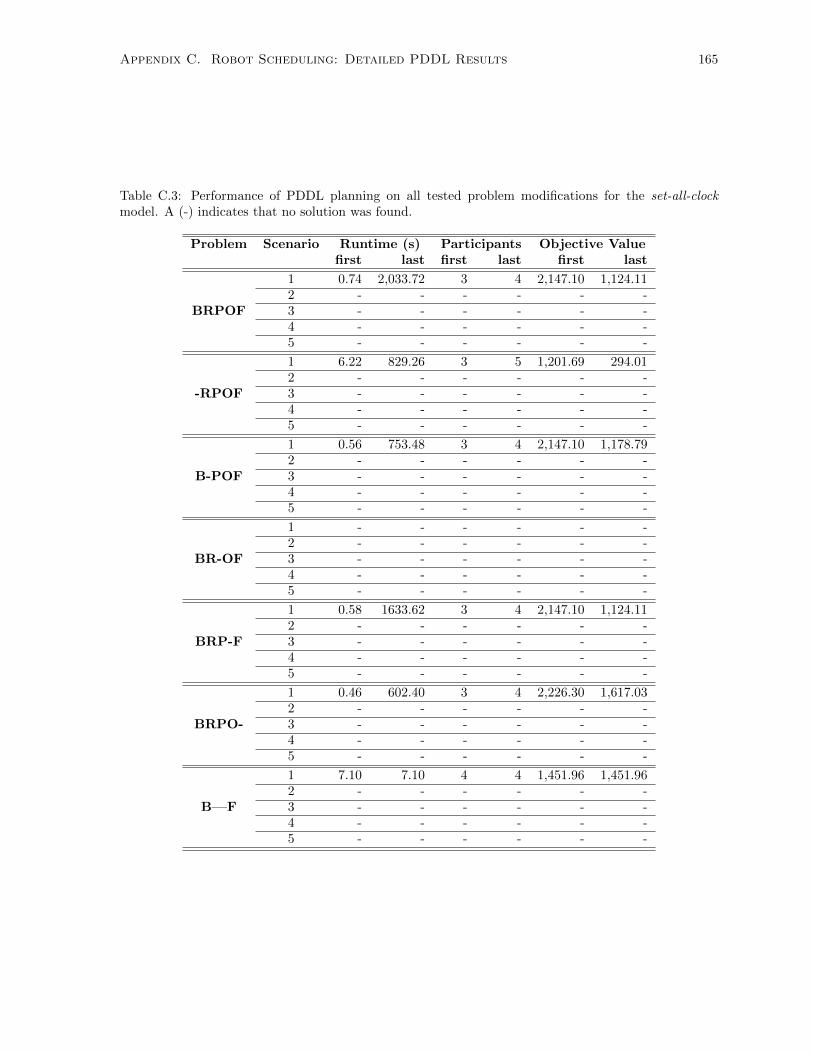
Appendix C. Robot Scheduling: Detailed PDDL Results 165
Table C.3: Performance of PDDL planning on all tested problem modifications for the set-all-clockmodel. A (-) indicates that no solution was found.
Problem Scenario Runtime (s) Participants Objective Valuefirst last first last first last
1 0.74 2,033.72 3 4 2,147.10 1,124.112 - - - - - -
BRPOF 3 - - - - - -4 - - - - - -5 - - - - - -
1 6.22 829.26 3 5 1,201.69 294.012 - - - - - -
-RPOF 3 - - - - - -4 - - - - - -5 - - - - - -
1 0.56 753.48 3 4 2,147.10 1,178.792 - - - - - -
B-POF 3 - - - - - -4 - - - - - -5 - - - - - -
1 - - - - - -2 - - - - - -
BR-OF 3 - - - - - -4 - - - - - -5 - - - - - -
1 0.58 1633.62 3 4 2,147.10 1,124.112 - - - - - -
BRP-F 3 - - - - - -4 - - - - - -5 - - - - - -
1 0.46 602.40 3 4 2,226.30 1,617.032 - - - - - -
BRPO- 3 - - - - - -4 - - - - - -5 - - - - - -
1 7.10 7.10 4 4 1,451.96 1,451.962 - - - - - -
B—F 3 - - - - - -4 - - - - - -5 - - - - - -
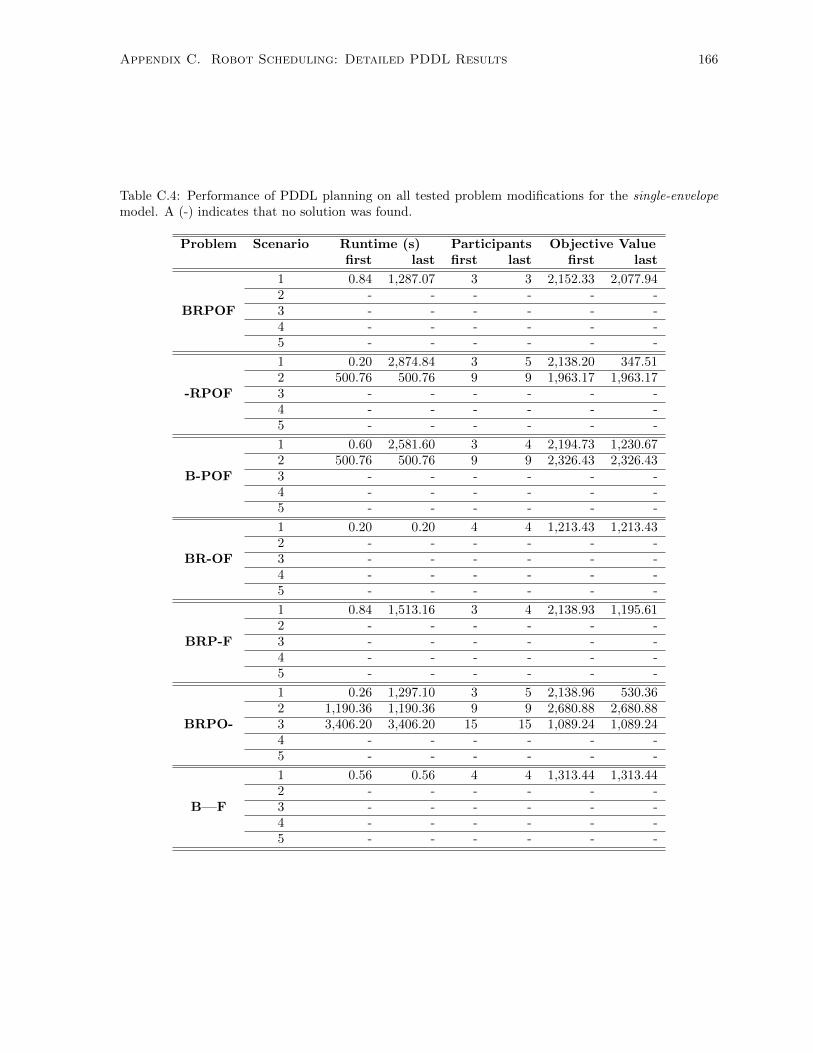
Appendix C. Robot Scheduling: Detailed PDDL Results 166
Table C.4: Performance of PDDL planning on all tested problem modifications for the single-envelopemodel. A (-) indicates that no solution was found.
Problem Scenario Runtime (s) Participants Objective Valuefirst last first last first last
1 0.84 1,287.07 3 3 2,152.33 2,077.942 - - - - - -
BRPOF 3 - - - - - -4 - - - - - -5 - - - - - -
1 0.20 2,874.84 3 5 2,138.20 347.512 500.76 500.76 9 9 1,963.17 1,963.17
-RPOF 3 - - - - - -4 - - - - - -5 - - - - - -
1 0.60 2,581.60 3 4 2,194.73 1,230.672 500.76 500.76 9 9 2,326.43 2,326.43
B-POF 3 - - - - - -4 - - - - - -5 - - - - - -
1 0.20 0.20 4 4 1,213.43 1,213.432 - - - - - -
BR-OF 3 - - - - - -4 - - - - - -5 - - - - - -
1 0.84 1,513.16 3 4 2,138.93 1,195.612 - - - - - -
BRP-F 3 - - - - - -4 - - - - - -5 - - - - - -
1 0.26 1,297.10 3 5 2,138.96 530.362 1,190.36 1,190.36 9 9 2,680.88 2,680.88
BRPO- 3 3,406.20 3,406.20 15 15 1,089.24 1,089.244 - - - - - -5 - - - - - -
1 0.56 0.56 4 4 1,313.44 1,313.442 - - - - - -
B—F 3 - - - - - -4 - - - - - -5 - - - - - -

Appendix C. Robot Scheduling: Detailed PDDL Results 167
Table C.5: Performance of PDDL planning on all tested problem modifications for the min-add-envelopemodel. A (-) indicates that no solution was found.
Problem Scenario Runtime (s) Participants Objective Valuefirst last first last first last
1 0.84 1,287.07 3 3 2,152.333 2,077.942 - - - - - -
BRPOF 3 - - - - - -4 - - - - - -5 - - - - - -
1 0.98 65.62 3 3 2,161.24 2,126.012 - - - - - -
-RPOF 3 - - - - - -4 - - - - - -5 - - - - - -
1 1.12 249.46 3 3 2,147.10 2,071.932 - - - - - -
B-POF 3 - - - - - -4 - - - - - -5 - - - - - -
1 - - - - - -2 - - - - - -
BR-OF 3 - - - - - -4 - - - - - -5 - - - - - -
1 1.04 1,013.14 3 3 2,152.33 2,077.942 - - - - - -
BRP-F 3 - - - - - -4 - - - - - -5 - - - - - -
1 0.22 1,269.80 3 4 2,261.10 1,620.542 - - - - - -
BRPO- 3 - - - - - -4 - - - - - -5 - - - - - -
1 - - - - - -2 - - - - - -
B—F 3 - - - - - -4 - - - - - -5 - - - - - -

Appendix C. Robot Scheduling: Detailed PDDL Results 168
Table C.6: Performance of PDDL planning on all tested problem modifications for the set-all-envelopemodel. A (-) indicates that no solution was found.
Problem Scenario Runtime (s) Participants Objective Valuefirst last first last first last
1 0.76 943.56 3 3 2,152.33 2,077.942 - - - - - -
BRPOF 3 - - - - - -4 - - - - - -5 - - - - - -
1 4.28 3,021.76 3 4 2,109.80 1,102.982 - - - - - -
-RPOF 3 - - - - - -4 - - - - - -5 - - - - - -
1 0.78 3336.24 3 4 2,147.10 1,168.812 - - - - - -
B-POF 3 - - - - - -4 - - - - - -5 - - - - - -
1 - - - - - -2 - - - - - -
BR-OF 3 - - - - - -4 - - - - - -5 - - - - - -
1 1.24 769.30 3 3 2,152.33 2,077.942 - - - - - -
BRP-F 3 - - - - - -4 - - - - - -5 - - - - - -
1 0.42 721.80 3 4 2,261.14 1,620.542 - - - - - -
BRPO- 3 - - - - - -4 - - - - - -5 - - - - - -
1 - - - - - -2 - - - - - -
B—F 3 - - - - - -4 - - - - - -5 - - - - - -
Bibliography
[1] T. Achterberg. Conflict analysis in mixed integer programming. Discrete Optimization, 4(1):4–20,
2007.
[2] S. H. Adachi and M. P. Henderson. Application of quantum annealing to training of deep neural
networks. arXiv:1510.06356, 2015.
[3] J. Adams, E. Balas, and D. Zawack. The shifting bottleneck procedure for job shop scheduling.
Management science, 34(3):391–401, 1988.
[4] I. Adiri, J. Bruno, E. Frostig, and A. R. Kan. Single machine flow-time scheduling with a single
breakdown. Acta Informatica, 26(7):679–696, 1989.
[5] A. Aggoun and N. Beldiceanu. Extending chip in order to solve complex scheduling and placement
problems. Mathematical and computer modelling, 17(7):57–73, 1993.
[6] I. Al-Azzoni and D. G. Down. Linear programming-based affinity scheduling of independent tasks
on heterogeneous computing systems. IEEE Transactions on Parallel and Distributed Systems,
19(12):1671–1682, 2008.
[7] R. Alami, R. Chatila, S. Fleury, M. Ghallab, and F. Ingrand. An architecture for autonomy. The
International Journal of Robotics Research, 17(4):315–337, 1998.
[8] S. Andradottir, H. Ayhan, and D. G. Down. Dynamic server allocation for queueing networks with
flexible servers. Operations Research, 51(6):952–968, 2003.
[9] M. Aramon Bajestani and J. C. Beck. Scheduling a dynamic aircraft repair shop with limited
repair resources. Journal of Artificial Intelligence Research, 47:35–70, 2013.
[10] S. Arora, D. Karger, and M. Karpinski. Polynomial time approximation schemes for dense instances
of np-hard problems. In Proceedings of the twenty-seventh annual ACM symposium on Theory of
computing, pages 284–293. ACM, 1995.
[11] F. Bacchus and F. Kabanza. Using temporal logics to express search control knowledge for planning.
Artificial Intelligence, 116(1):123 – 191, 2000.
[12] J. Bajada, M. Fox, and D. Long. Temporal plan quality improvement and repair using local search.
In STAIRS 2014: Proceedings of the 7th European Starting AI Researcher Symposium, volume 264,
pages 41–50. IOS Press, 2014.
169

BIBLIOGRAPHY 170
[13] M. A. Bajestani and J. C. Beck. A two-stage coupled algorithm for an integrated maintenance
planning and flowshop scheduling problem with deteriorating machines. Journal of Scheduling,
18(5):471–486, 2015.
[14] K. R. Baker and J. W. M. Bertrand. A comparison of due-date selection rules. AIIE Transactions,
13(2):123–131, 1981.
[15] K. R. Baker and J. J. Kanet. Job shop scheduling with modified due dates. Journal of Operations
Management, 4(1):11–22, 1983.
[16] K. R. Baker and D. Trietsch. Principles of Sequencing and Scheduling. Wiley Publishing, 2009.
[17] H. H. Balci and J. F. Valenzuela. Scheduling electric power generators using particle swarm
optimization combined with the lagrangian relaxation method. International Journal of Applied
Mathematics and Computer Science, 14(3):411–422, 2004.
[18] M. R. Banks, L. M. Willoughby, and W. A. Banks. Animal-assisted therapy and loneliness in
nursing homes: use of robotic versus living dogs. Journal of the American Medical Directors
Association, 9(3):173–177, 2008.
[19] P. Baptiste, P. Laborie, C. Le Pape, and W. Nuijten. Constraint-based scheduling and planning.
Foundations of Artificial Intelligence, 2:761–799, 2006.
[20] P. Baptiste, C. Le Pape, and W. Nuijten. Constraint-based scheduling: applying constraint pro-
gramming to scheduling problems, volume 39. Springer Science & Business Media, 2012.
[21] J. F. Bard and H. W. Purnomo. Preference scheduling for nurses using column generation. Euro-
pean Journal of Operational Research, 164(2):510–534, 2005.
[22] C. Barnhart, E. L. Johnson, G. L. Nemhauser, M. W. Savelsbergh, and P. H. Vance. Branch-and-
price: Column generation for solving huge integer programs. Operations research, 46(3):316–329,
1998.
[23] J. Barreiro, M. Boyce, M. Do, J. Frank, M. Iatauro, T. Kichkaylo, P. Morris, J. Ong, E. Re-
molina, T. Smith, and D. Smith. EUROPA: A platform for AI planning, scheduling, constraint
programming, and optimization. In Proceedings of the 4th International Competition on Knowledge
Engineering for Planning and Scheduling (ICKEPS), 2012.
[24] R. Bartak. Visopt shopfloor: On the edge of planning and scheduling. In Principles and Practice
of Constraint Programming-CP 2002, pages 587–602. Springer, 2002.
[25] R. Bartak, M. A. Salido, and F. Rossi. New trends in constraint satisfaction, planning, and
scheduling: a survey. The Knowledge Engineering Review, 25(03):249–279, 2010.
[26] S. D. Bartlett. Atomic physics: A milestone in quantum computing. Nature, 536(7614):35–36,
2016.
[27] J. C. Beck, A. J. Davenport, E. D. Davis, and M. S. Fox. The odo project: Toward a unified basis
for constraint-directed scheduling. Journal of Scheduling, 1(2):89–125, 1998.

BIBLIOGRAPHY 171
[28] J. C. Beck and M. S. Fox. Constraint-directed techniques for scheduling alternative activities.
Artificial Intelligence, 121(1):211–250, 2000.
[29] J. C. Beck and L. Perron. Discrepancy-bounded depth first search. In Proceedings of the Second
International Workshop on Integration of AI and OR Techniques in Constraint Programming for
Combinatorial Optimization Problems (CP-AI-OR 2000), pages 8–10, 2000.
[30] J. C. Beck, P. Prosser, and R. J. Wallace. Trying again to fail-first. In Recent Advances in
Constraints, pages 41–55. Springer, 2004.
[31] J. C. Beck and P. Refalo. A hybrid approach to scheduling with earliness and tardiness costs.
Annals of Operations Research, 118(1-4):49–71, 2003.
[32] M. Beetz and M. Bennewitz. Planning, scheduling, and plan execution for autonomous robot
office couriers. In Integrating Planning, Scheduling and Execution in Dynamic and Uncertain
Environments, volume Workshop Notes, pages 98–02, 1998.
[33] J. F. Benders. Partitioning procedures for solving mixed-variables programming problems. Nu-
merische mathematik, 4(1):238–252, 1962.
[34] M. Benedetti, J. Realpe-Gomez, R. Biswas, and A. Perdomo-Ortiz. Estimation of effective tem-
peratures in a quantum annealer and its impact in sampling applications: A case study towards
deep learning applications. arXiv:1510.07611, 2015.
[35] J. Benton, A. J. Coles, and A. I. Coles. Temporal planning with preferences and time-dependent
continuous costs. In Proceedings of the Twenty Second International Conference on Automated
Planning and Scheduling (ICAPS-12), pages 2–10, June 2012.
[36] D. Bergman, A. A. Cire, and W.-J. van Hoeve. Improved constraint propagation via lagrangian
decomposition. In International Conference on Principles and Practice of Constraint Programming,
pages 30–38. Springer, 2015.
[37] D. Bergman, A. A. Cire, and W.-J. van Hoeve. Lagrangian bounds from decision diagrams.
Constraints, 20(3):346–361, 2015.
[38] J. L. Berral, I. Goiri, R. Nou, F. Julia, J. Guitart, R. Gavalda, and J. Torres. Towards energy-
aware scheduling in data centers using machine learning. In Proceedings of the 1st International
Conference on energy-Efficient Computing and Networking, pages 215–224. ACM, 2010.
[39] T. Berthold. Measuring the impact of primal heuristics. Operations Research Letters, 41(6):611–
614, 2013.
[40] D. Bertsimas and J. N. Tsitsiklis. Introduction to linear optimization, volume 6. Athena Scientific
Belmont, MA, 1997.
[41] D. Bertsimas and R. Weismantel. Optimization over integers, volume 13. Dynamic Ideas Belmont,
2005.
[42] D. Biskup, J. Herrmann, and J. N. Gupta. Scheduling identical parallel machines to minimize
total tardiness. International Journal of Production Economics, 115(1):134–142, 2008.

BIBLIOGRAPHY 172
[43] S. Boixo, T. F. Rønnow, S. V. Isakov, Z. Wang, D. Wecker, D. A. Lidar, J. M. Martinis, and
M. Troyer. Evidence for quantum annealing with more than one hundred qubits. Nature Physics,
10(3):218–224, 2014.
[44] S. Boixo, V. N. Smelyanskiy, A. Shabani, S. V. Isakov, M. Dykman, V. S. Denchev, M. Amin,
A. Smirnov, M. Mohseni, and H. Neven. Computational role of collective tunneling in a quantum
annealer. arXiv:1411.4036, 2014.
[45] B. Bonet and H. Geffner. Planning as heuristic search. Artificial Intelligence, 129(1):5–33, 2001.
[46] K. E. Booth, T. T. Tran, and J. C. Beck. Logic-based decomposition methods for the travel-
ling purchaser problem. In International Conference on AI and OR Techniques in Constriant
Programming for Combinatorial Optimization Problems, pages 55–64. Springer, 2016.
[47] K. E. Booth, T. T. Tran, G. Nejat, and J. C. Beck. Mixed-integer and constraint programming
techniques for mobile robot task planning. IEEE Robotics and Automation Letters, 1(1):500–507,
2016.
[48] A. Borodin and R. El-Yaniv. Online computation and competitive analysis. cambridge university
press, 2005.
[49] E. H. Bowman. The schedule-sequencing problem. Operations Research, 7(5):621–624, 1959.
[50] C. B. Browne, E. Powley, D. Whitehouse, S. M. Lucas, P. I. Cowling, P. Rohlfshagen, S. Tavener,
D. Perez, S. Samothrakis, and S. Colton. A survey of monte carlo tree search methods. IEEE
Transactions on Computational Intelligence and AI in Games, 4(1):1–43, 2012.
[51] C. Burt, N. Lipovetzky, A. Pearce, and P. Stuckey. Approximate uni-directional benders decom-
position. In Proceedings of the 29th AAAI Conference on Artificial Intelligence Workshop on
Planning Search and Optimization (PlanSOpt-15), pages 1–8, 2015.
[52] J. Cai, W. G. Macready, and A. Roy. A practical heuristic for finding graph minors.
arXiv:1406.2741, 2014.
[53] J. D. Camm, A. S. Raturi, and S. Tsubakitani. Cutting big m down to size. Interfaces, 20(5):61–66,
1990.
[54] J. Carlier. The one-machine sequencing problem. European Journal of Operational Research,
11(1):42–47, 1982.
[55] V. Cerny. Thermodynamical approach to the traveling salesman problem: An efficient simulation
algorithm. Journal of optimization theory and applications, 45(1):41–51, 1985.
[56] A. Cesta, G. Cortellessa, R. Rasconi, F. Pecora, M. Scopelliti, and L. Tiberio. Monitoring el-
derly people with the robocare domestic environment: Interaction synthesis and user evaluation.
Computational Intelligence, 27(1):60–82, 2011.
[57] A. Cesta, S. Fratini, and F. Pecora. Unifying planning and scheduling as timelines in a component-
based perspective. Archives of Control Science, 18(2):231–271, 2008.

BIBLIOGRAPHY 173
[58] Z.-L. Chen and W. B. Powell. Solving parallel machine scheduling problems by column generation.
INFORMS Journal on Computing, 11(1):78–94, 1999.
[59] C.-P. Cheng, C.-W. Liu, and C.-C. Liu. Unit commitment by lagrangian relaxation and genetic
algorithms. IEEE transactions on power systems, 15(2):707–714, 2000.
[60] V. Choi. Minor-embedding in adiabatic quantum computation: II. minor-universal graph design.
Quantum Information Processing, 10(3):343–353, 2011.
[61] Y. Chu and Q. Xia. A hybrid algorithm for a class of resource constrained scheduling problems.
In Proceedings of the 2nd Conference on Integration of AI and OR Techniques in Constraint
Programming for Combinatorial Optimization Problems, pages 110–124. Springer, 2005.
[62] A. A. Cire and J. N. Hooker. A heuristic logic-based benders method for the home health care
problem. In Presented at Matheuristics 2012, 2012.
[63] A. J. Coles, A. Coles, M. Fox, and D. Long. Forward-chaining partial-order planning. In Proceedings
of the 20th International Conference on Automated Planning and Scheduling (ICAPS), pages 42–
49, 2010.
[64] A. J. Coles, A. I. Coles, M. Fox, and D. Long. Colin: Planning with continuous linear numeric
change. Journal of Artificial Intelligence Research, 44(1):1–96, 2012.
[65] A. J. Coles, A. I. Coles, M. Fox, and D. Long. A hybrid LP-RPG heuristic for modelling numeric
resource flows in planning. Journal of Artificial Intelligence Research, 46:343–412, 2013.
[66] B. Coltin, M. M. Veloso, and R. Ventura. Dynamic user task scheduling for mobile robots. In
Automated Action Planning for Autonomous Mobile Robots, pages 1–9, 2011.
[67] R. W. Conway. Priority dispatching and work-in-process inventory in a job shop. Journal of
Industrial Engineering, 16(2):123, 1965.
[68] R. Coulom. Efficient selectivity and backup operators in monte-carlo tree search. In International
Conference on Computers and Games, pages 72–83. Springer, 2006.
[69] J. Culberson, A. Beacham, and D. Papp. Hiding our colors. In CP95 Workshop on Studying and
Solving Really Hard Problems, pages 31–42. Citeseer, 1995.
[70] W. A. Cushing and S. Kambhampati. When is temporal planning really temporal. In Proceedigns
of the 20th International Joint Conference On Artificial Intelligence, pages 1852–1859, 2007.
[71] J. G. Dai and S. P. Meyn. Stability and convergence of moments for multiclass queueing networks
via fluid limit models. IEEE Transactions on Automatic Control, 40(11):1889–1904, 1995.
[72] Q.-V. Dang, I. Nielsen, K. Steger-Jensen, and O. Madsen. Scheduling a single mobile robot for
part-feeding tasks of production lines. Journal of Intelligent Manufacturing, 25(6):1–17, 2013.
[73] G. B. Dantzig and M. N. Thapa. Linear programming 2: theory and extensions. Springer Science
& Business Media, 2006.
[74] A. Das and B. K. Chakrabarti. Colloquium: Quantum annealing and analog quantum computation.
Rev. Mod. Phys., 80:1061–1081, 2008.

BIBLIOGRAPHY 174
[75] R. Dechter. Constraint processing. Morgan Kaufmann, 2003.
[76] G. Desaulniers, J. Desrosiers, and M. M. Solomon. Column generation, volume 5. Springer Science
& Business Media, 2006.
[77] D. G. Down and M. E. Lewis. Dynamic load balancing in parallel queueing systems: Stability and
optimal control. European Journal of Operational Research, 168(2):509–519, 2006.
[78] F. Dvorak, A. Bit-Monnot, F. Ingrand, and M. Ghallab. A flexible anml actor and planner
in robotics. In Proceedings of the 24th International Conference on Automated Planning and
Scheduling (ICAPS) Workshop on Planning and Robotics (PlanRob), 2014.
[79] S. Edelkamp and J. Hoffmann. PDDL2.2: the language for the classical part of the 4th international
planning competition. 4th International Planning Competition (IPC04), at ICAPS04, 2004.
[80] H. El Sakkout and M. Wallace. Probe backtrack search for minimal perturbation in dynamic
scheduling. Constraints, 5(4):359–388, 2000.
[81] T. Estlin, R. Castano, R. Anderson, D. Gaines, F. Fisher, and M. Judd. Learning and planning for
mars rover science. In Proc. IJCAI Workshop on Issues in Designing Physical Agents for Dynamic
Real Time Environments: World Modelling, Planning, Learning and Communicating, 2003.
[82] T. Estlin, D. Gaines, C. Chouinard, R. Castano, B. Bornstein, M. Judd, I. Nesnas, and R. An-
derson. Increased mars rover autonomy using AI planning, scheduling and execution. In Robotics
and Automation, 2007 IEEE International Conference on, pages 4911–4918. IEEE, 2007.
[83] E. Farhi, J. Goldstone, S. Gutmann, and M. Sipser. Quantum computation by adiabatic evolution.
arXiv:quant-ph/0001106, Jan. 2000.
[84] E. Farhi, J. Goldstone, S. Gutmann, and M. Sipser. Quantum computation by adiabatic evolution.
arXiv preprint quant-ph/0001106, 2000.
[85] M. Fazel-Zarandi and J. Beck. Using logic-based Benders decomposition to solve the capacity and
distance constrained plant location problem. INFORMS Journal on Computing, 24:399–415, 2012.
[86] M. Fazel-Zarandi, O. Berman, and J. Beck. Solving a stochastic facility location/fleet management
problem with logic-based Benders decomposition. IIE Transactions, 45(8):896–911, 2013.
[87] J. Fdez-Olivares, J. A. Cozar, and L. Castillo. Oncotheraper: Clinical decision support for oncology
therapy planning based on temporal hierarchical tasks networks. In Knowledge Management for
Health Care Procedures, volume 5626, pages 25–41. Springer, 2009.
[88] Z. Feldman and C. Domshlak. Simple regret optimization in online planning for markov decision
processes. Journal of Artificial Intelligence Research, 51:165–205, 2014.
[89] M. L. Fisher. The lagrangian relaxation method for solving integer programming problems. Man-
agement science, 27(1):1–18, 1981.
[90] F. Focacci, A. Lodi, and M. Milano. Optimization-oriented global constraints. Constraints, 7(3-
4):351–365, 2002.

BIBLIOGRAPHY 175
[91] L. R. Ford Jr and D. R. Fulkerson. A suggested computation for maximal multi-commodity network
flows. Management Science, 5(1):97–101, 1958.
[92] M. Fox and D. Long. Modelling mixed discrete-continuous domains for planning. Journal of
Artificial Intelligence Research, 27:235–297, 2006.
[93] J. Frank. An intelligent agent for autonomous lunar exploration. In Proceedings of the 18th In-
ternational Conference on Automated Planning and Scheduling (ICAPS) Workshop on Scheduling
and Planning Application, pages 1–8, 2008.
[94] E. C. Freuder. In pursuit of the holy grail. Constraints, 2(1):57–61, 1997.
[95] A. M. Frisch, W. Harvey, C. Jefferson, B. Martınez-Hernandez, and I. Miguel. Essence: A con-
straint language for specifying combinatorial problems. Constraints, 13(3):268–306, 2008.
[96] C. Fritz and S. A. McIlraith. Planning in the face of frequent exogenous events. In Online Poster
Proceedings of the 18th International Conference on Automated Planning and Scheduling (ICAPS),
pages 14–18, 2008.
[97] T. Gabriel Crainic and J.-M. Rousseau. The column generation principle and the airline crew
scheduling problem. INFOR: Information Systems and Operational Research, 25(2):136–151, 1987.
[98] D. M. Gaines, T. Estlin, C. Chouinard, R. Castano, A. Castano, B. Bornstein, R. C. Anderson,
M. Judd, I. Nesnas, and G. Rabideau. Opportunistic planning and execution for planetary explo-
ration. In Proceedings of the 16th International Conference on Automated Planning and Scheduling
(ICAPS), pages 1–3, 2006.
[99] A. Gandhi, M. Harchol-Balter, and M. A. Kozuch. Are sleep states effective in data centers? In
International Green Computing Conference (IGCC), pages 1–10. IEEE, 2012.
[100] M. R. Garey and D. S. Johnson. A guide to the theory of np-completeness. WH Freemann, New
York, 1979.
[101] M. R. Garey, D. S. Johnson, and R. E. Tarjan. The planar hamiltonian circuit problem is np-
complete. SIAM Journal on Computing, 5(4):704–714, 1976.
[102] A. Gerevini, A. Saetti, I. Serina, and P. Toninelli. LPG-TD: a fully automated planner for PDDL2.2
domains. In In Proceedings of the 14th International Conference on Automated Planning and
Scheduling (ICAPS) International Planning Competition abstracts, 2004. Booklet of the system
demo section.
[103] M. Ghallab, A. Howe, C. Knoblock, D. McDermott, A. Ram, M. Veloso, D. Weld, and D. Wilkins.
PDDL—The Planning Domain Definition Language, 1998.
[104] M. Ghallab, D. Nau, and P. Traverso. Automated planning: theory & practice. Elsevier, 2004.
[105] A. Ghodsi, M. Zaharia, B. Hindman, A. Konwinski, S. Shenker, and I. Stoica. Dominant resource
fairness: Fair allocation of multiple resource types. In Proceedings of the 8th USENIX conference
on Networked systems design and implementation, volume 11, pages 323–336, 2011.

BIBLIOGRAPHY 176
[106] P. C. Gilmore and R. E. Gomory. A linear programming approach to the cutting-stock problem.
Operations research, 9(6):849–859, 1961.
[107] V. Goel, I. E. Grossmann, A. S. El-Bakry, and E. L. Mulkay. A novel branch and bound algo-
rithm for optimal development of gas fields under uncertainty in reserves. Computers & chemical
engineering, 30(6):1076–1092, 2006.
[108] R. L. Graham, E. L. Lawler, J. K. Lenstra, and A. R. Kan. Optimization and approximation in
deterministic sequencing and scheduling: a survey. Annals of discrete mathematics, 5:287–326,
1979.
[109] R. Grandl, G. Ananthanarayanan, S. Kandula, S. Rao, and A. Akella. Multi-resource packing for
cluster schedulers. In Proceedings of the 2014 ACM conference on SIGCOMM, pages 455–466.
ACM, 2014.
[110] G. H. Graves and C.-Y. Lee. Scheduling maintenance and semiresumable jobs on a single machine.
Naval Research Logistics (NRL), 46(7):845–863, 1999.
[111] M. Guazzone, C. Anglano, and M. Canonico. Exploiting vm migration for the automated power
and performance management of green cloud computing systems. In Energy Efficient Data Centers,
volume 7396, pages 81–92. Springer, 2012.
[112] B. Guenter, N. Jain, and C. Williams. Managing cost, performance, and reliability tradeoffs for
energy-aware server provisioning. In INFOCOM, 2011 Proceedings IEEE, pages 1332–1340. IEEE,
2011.
[113] G. Gupta, W. Malik, and Y. C. Jung. A mixed integer linear program for airport departure
scheduling. In 9th AIAA aviation technology, integration, and operations conference (ATIO),
pages 21–23, 2009.
[114] R. M. Haralick and G. L. Elliott. Increasing tree search efficiency for constraint satisfaction
problems. Artificial intelligence, 14(3):263–313, 1980.
[115] W. D. Harvey and M. L. Ginsberg. Limited discrepancy search. In Proceedings of the Fourteenth
International Joint Conference on Artificial Intelligence (IJCAI), pages 607–615, 1995.
[116] R. Haupt. A survey of priority rule-based scheduling. Operations-Research-Spektrum, 11(1):3–16,
1989.
[117] Y.-T. He and D. G. Down. Limited choice and locality considerations for load balancing. Perfor-
mance Evaluation, 65(9):670–687, 2008.
[118] S. Heinz and J. C. Beck. Reconsidering mixed integer programming and MIP-based hybrids for
scheduling. In International Conference on Integration of Artificial Intelligence (AI) and Opera-
tions Research (OR) Techniques in Constraint Programming, pages 211–227. Springer, 2012.
[119] S. Heinz, W.-Y. Ku, and J. C. Beck. Recent improvements using constraint integer programming
for resource allocation and scheduling. In Integration of AI and OR Techniques in Constraint
Programming for Combinatorial Optimization Problems, pages 12–27. Springer, 2013.

BIBLIOGRAPHY 177
[120] S. Heinz, J. Schulz, and J. C. Beck. Using dual presolving reductions to reformulate cumulative
constraints. Constraints, 18(2):166–201, 2013.
[121] J. A. Hendler, A. Tate, and M. Drummond. Ai planning: Systems and techniques. AI magazine,
11(2):61, 1990.
[122] C. Hewitt. Procedural embedding of knowledge in planner. In Proceedings of the 2nd international
joint conference on Artificial intelligence, pages 167–182, 1971.
[123] J. Hoffmann and B. Nebel. The ff planning system: Fast plan generation through heuristic search.
Journal of Artificial Intelligence Research, 14:253–302, 2001.
[124] O. Holthaus and C. Rajendran. Efficient dispatching rules for scheduling in a job shop. Interna-
tional Journal of Production Economics, 48(1):87–105, 1997.
[125] J. Hooker. Verifying logic circuits by Benders decomposition. Principles and Practice of Constraint
Programming: The Newport Papers, MIT Press, Cambridge, MA, pages 267–288, 1995.
[126] J. Hooker. Logic-based Methods for Optimization. Wiley, 2000.
[127] J. N. Hooker and G. Ottosson. Logic-based benders decomposition. Mathematical Programming,
96(1):33–60, 2003.
[128] C.-W. Hsu and B. W. Wah. The SGPlan planning system in IPC-6. In In the booklet of the
International Planning Competition (IPC), International Conference on Planning and Scheduling
(ICAPS), 2008.
[129] M. Isard, V. Prabhakaran, J. Currey, U. Wieder, K. Talwar, and A. Goldberg. Quincy: fair
scheduling for distributed computing clusters. In Proceedings of the ACM SIGOPS 22nd symposium
on Operating systems principles, pages 261–276. ACM, 2009.
[130] F. Ivankovic, P. Haslum, S. Thiebaux, V. Shivashankar, and D. S. Nau. Optimal planning with
global numerical state constraints. In Proceedings of 24th International Conference on Automated
Planning and Scheduling (ICAPS), pages 145–153, 2014.
[131] J. R. Jackson. Scheduling a production line to minimize maximum tardiness. Technical report,
DTIC Document, 1955.
[132] A. Jain, J. Guineau, C. Lim, W. Lincoln, M. Pomerantz, G. Sohl, and R. Steele. Roams: Plane-
tary surface rover simulation environment. In International Symposium on Artificial Intelligence,
Robotics and Automation in Space (i-SAIRAS 2003), pages 1–8, 2003.
[133] R. Jain, D.-M. Chiu, and W. Hawe. A quantitative measure of fairness and discrimination for
resource allocation in shared computer systems. Digital Equipment Corporation Research Technical
Report TR-301, pages 1–37, 1984.
[134] B. Jaumard, F. Semet, and T. Vovor. A generalized linear programming model for nurse scheduling.
European journal of operational research, 107(1):1–18, 1998.

BIBLIOGRAPHY 178
[135] S. Jimenez, A. Jonsson, and H. Palacios. Temporal planning with required concurrency using
classical planning. In Proceedings of the 25th International Conference on Automated Planning
and Scheduling (ICAPS), 2015. In press.
[136] M. W. Johnson, M. H. S. Amin, S. Gildert, and et al. Quantum annealing with manufactured
spins. Nature, 473:194–198, 2011.
[137] S. M. Johnson. Optimal two-and three-stage production schedules with setup times included.
Naval research logistics quarterly, 1(1):61–68, 1954.
[138] C. A. Kaskavelis and M. C. Caramanis. Efficient lagrangian relaxation algorithms for industry size
job-shop scheduling problems. IIE transactions, 30(11):1085–1097, 1998.
[139] V. Kats and E. Levner. Parametric algorithms for 2-cyclic robot scheduling with interval processing
times. Journal of Scheduling, 14(3):267–279, 2011.
[140] J. Kelley. The cutting-plane method for solving convex programs. Journal of the Society for
Industrial and Applied Mathematics, pages 703–712, 1960.
[141] J.-K. Kim, S. Shivle, H. J. Siegel, A. A. Maciejewski, T. D. Braun, M. Schneider, S. Tideman,
R. Chitta, R. B. Dilmaghani, R. Joshi, et al. Dynamically mapping tasks with priorities and
multiple deadlines in a heterogeneous environment. Journal of Parallel and Distributed Computing,
67(2):154–169, 2007.
[142] J. King, S. Yarkoni, M. M. Nevisi, J. P. Hilton, and C. C. McGeoch. Benchmarking a quantum
annealing processor with the time-to-target metric. arXiv preprint arXiv:1508.05087, 2015.
[143] S. Kirkpatrick, C. D. Gelatt, M. P. Vecchi, et al. Optimization by simmulated annealing. science,
220(4598):671–680, 1983.
[144] E. Kondili, C. Pantelides, R. Sargent, et al. A general algorithm for scheduling batch operations.
In PSE’88: Third International Symposium on Process Systems Engineering: In Affiliation with
CHEMECA 88, a Bicentennial Event; Sydney, Australia, 28 August-2 September, 1998; Preprints
of Papers, page 62. Institution of Engineers, Australia, 1988.
[145] S. Kosch and J. C. Beck. A new mip model for parallel-batch scheduling with non-identical job
sizes. In International Conference on AI and OR Techniques in Constriant Programming for
Combinatorial Optimization Problems, pages 55–70. Springer, 2014.
[146] W.-Y. Ku and J. C. Beck. Mixed integer programming models for job shop scheduling: A compu-
tational analysis. Computers & Operations Research, 73:165 – 173, 2016.
[147] J. Kvarnstrom and P. Doherty. Talplanner: A temporal logic based forward chaining planner.
Annals of Mathematics and Artificial Intelligence, 30(1-4):119–169, 2000.
[148] P. Laborie. Algorithms for propagating resource constraints in AI planning and scheduling: existing
approaches and new results. Artificial Intelligence, 143(2):151–188, 2003.
[149] P. Laborie. IBM ILOG CP Optimizer for detailed scheduling illustrated on three problems. In
Integration of AI and OR Techniques in Constraint Programming for Combinatorial Optimization
Problems, pages 148–162. Springer, 2009.

BIBLIOGRAPHY 179
[150] P. Laborie and J. Rogerie. Reasoning with conditional time-intervals. In FLAIRS conference,
pages 555–560, 2008.
[151] P. Laborie and J. Rogerie. Temporal linear relaxation in IBM ILOG CP Optimizer. Journal of
Scheduling, 19(4):391–400, 2016.
[152] G. Laporte and Y. Nobert. A cutting planes algorithm for the m-salesmen problem. Journal of
the Operational Research Society, 31(11):1017–1023, 1980.
[153] J. Larson, M. Johansson, and M. Carlsson. An integrated constraint programming approach to
scheduling sports leagues with divisional and round-robin tournaments. In International Con-
ference on AI and OR Techniques in Constriant Programming for Combinatorial Optimization
Problems, pages 144–158. Springer, 2014.
[154] A. M. Law, W. D. Kelton, and W. D. Kelton. Simulation modeling and analysis, volume 2.
McGraw-Hill New York, 1991.
[155] K. Le, R. Bianchini, J. Zhang, Y. Jaluria, J. Meng, and T. D. Nguyen. Reducing electricity cost
through virtual machine placement in high performance computing clouds. In Proceedings of the
International Conference for High Performance Computing, Networking, Storage and Analysis,
page 22. ACM, 2011.
[156] Y. H. Lee and M. Pinedo. Scheduling jobs on parallel machines with sequence-dependent setup
times. European Journal of Operational Research, 100(3):464–474, 1997.
[157] J. K. Lenstra, D. B. Shmoys, and E. Tardos. Approximation algorithms for scheduling unrelated
parallel machines. Mathematical programming, 46(1-3):259–271, 1990.
[158] C.-J. Liao and C.-T. You. An improved formulation for the job-shop scheduling problem. Journal
of the Operational Research Society, 43(11):1047–1054, 1992.
[159] D.-Y. Lin and S.-L. Hwang. Use of neural networks to achieve dynamic task allocation: a flexible
manufacturing system example. International Journal of Industrial Ergonomics, 24(3):281–298,
1999.
[160] Z. Liu, M. Lin, A. Wierman, S. H. Low, and L. L. Andrew. Greening geographical load balancing.
In Proceedings of the ACM SIGMETRICS Joint International Conference on Measurement and
Modeling of Computer Systems, pages 233–244. ACM, 2011.
[161] S. Lloyd. Least squares quantization in PCM. IEEE Transactions on Information Theory,
28(2):129–137, 1982.
[162] W.-Y. G. Louie, J. Li, T. Vaquero, and G. Nejat. A focus group study on the design considerations
and impressions of a socially assistive robot for long-term care. In Robot and Human Interactive
Communication, 2014 RO-MAN: The 23rd IEEE International Symposium on, pages 237–242.
IEEE, 2014.
[163] W.-Y. G. Louie, J. Li, T. Vaquero, and G. Nejat. Design considerations and impressions of
socially assistive robots for seniors living in long-term care facilities. In Human-Robot Interactions:
Principles, Technologies and Challenges. Nova Science Publishers, Inc, 2015.

BIBLIOGRAPHY 180
[164] W.-Y. G. Louie, J. Li, T. Vaquero, and G. Nejat. Socially assistive robots for seniors living
in residential care homes: User requirements and impressions. In Human-Robot Interactions:
Principles, Technologies and Challenges, pages 75–108. Nova Science Publishers, Inc, 2015.
[165] W.-Y. G. Louie, T. Vaquero, G. Nejat, and J. C. Beck. An autonomous assistive robot for plan-
ning, scheduling and facilitating multi-user activities. In Proceedings of the IEEE International
Conference on Robotics and Automation (ICRA), pages 5292–5298, 2014.
[166] M. E. Lubbecke and J. Desrosiers. Selected topics in column generation. Operations Research,
53(6):1007–1023, 2005.
[167] S. T. Maguluri, R. Srikant, and L. Ying. Heavy traffic optimal resource allocation algorithms for
cloud computing clusters. In Proceedings of the 24th International Teletraffic Congress, page 25.
International Teletraffic Congress, 2012.
[168] S. T. Maguluri, R. Srikant, and L. Ying. Stochastic models of load balancing and scheduling in
cloud computing clusters. In Proceedings IEEE INFOCOM, pages 702–710. IEEE, 2012.
[169] A. Malapert, C. Gueret, and L.-M. Rousseau. A constraint programming approach for a batch
processing problem with non-identical job sizes. European Journal of Operational Research,
221(3):533–545, 2012.
[170] Z. A. Mann. Allocation of virtual machines in cloud data centers–a survey of problem models and
optimization algorithms. ACM Computing Surveys, 48(1):1–31, 2015.
[171] A. S. Manne. On the job-shop scheduling problem. Operations Research, 8(2):219–223, 1960.
[172] R. K. Martin. Generating alternative mixed-integer programming models using variable redefini-
tion. Operations Research, 35(6):820–831, 1987.
[173] E. Marzal, L. Sebastia, and E. Onaindia. On the use of temporal landmarks for planning with
deadlines. In Twenty-Fourth International Conference on Automated Planning and Scheduling,
pages 172–180, 2014.
[174] L. Mercier and P. Van Hentenryck. Edge finding for cumulative scheduling. INFORMS Journal
on Computing, 20(1):143–153, 2008.
[175] A. Mishra, J. Hellerstein, W. Cirne, and C. Das. Towards characterizing cloud backend workloads:
insights from Google compute clusters. ACM SIGMETRICS Performance Evaluation Review,
37(4):34–41, 2010.
[176] S. Mittal and B. Falkenhainer. Dynamic constraint satisfaction. In Proceedings of the Eighth
National Conference on Artificial Intelligence, pages 25–32, 1990.
[177] S. C. Mohamed and G. Nejat. Autonomous search by a socially assistive robot in a residential care
environment for multiple elderly users using group activity preferences. In Proceedings of the 26th
International Conference on Automated Planning and Scheduling (ICAPS) Workshop on Planning
and Robotics (PlanRob), pages 58–66, 2016.
[178] Y. Monden. Toyota production system: an integrated approach to just-in-time. CRC Press, 2011.

BIBLIOGRAPHY 181
[179] C. Muise, J. C. Beck, and S. A. McIlraith. Flexible Execution of Partial Order Plans With Temporal
Constraints. In International Joint Conference On Artificial Intelligence, pages 2328–2335, 2013.
[180] C. Muise, J. C. Beck, and S. A. McIlraith. Optimal partial-order plan relaxation via maxsat.
Journal of Artificial Intelligence Research, 57:113–149, 2016.
[181] C. Muise, V. Belle, and S. A. McIlraith. Computing contingent plans via fully observable non-
deterministic planning. Models and Paradigms for Planning under Uncertainty: a Broad Perspec-
tive, pages 2322–2329, 2014.
[182] B. Naderi, S. F. Ghomi, and M. Aminnayeri. A high performing metaheuristic for job shop
scheduling with sequence-dependent setup times. Applied Soft Computing, 10(3):703–710, 2010.
[183] D. S. Nau, T.-C. Au, O. Ilghami, U. Kuter, J. W. Murdock, D. Wu, and F. Yaman. Shop2: An
htn planning system. J. Artif. Intell. Res.(JAIR), 20:379–404, 2003.
[184] M. Nielsen and I. Chuang. Quantum Computing and Quantum Information. Cambridge University
Press, Cambridge, 2001.
[185] P. Nightingale and A. Rendl. Essence’ description 1.6. 4. arXiv preprint arXiv:1601.02865, 2016.
[186] N. J. Nilsson. Shakey the robot. Technical report, DTIC Document, 1984.
[187] R. O’Donovan, R. Uzsoy, and K. N. McKay. Predictable scheduling of a single machine with
breakdowns and sensitive jobs. International Journal of Production Research, 37(18):4217–4233,
1999.
[188] B. O’Gorman, E. G. Rieffel, M. Do, D. Venturelli, and J. Frank. Compiling planning into quantum
optimization problems: a comparative study. Constraint Satisfaction Techniques for Planning and
Scheduling Problems (COPLAS-15), page 11, 2015.
[189] OMG. OMG unified modeling language specification. Version 2.0, 2005.
[190] D. Ouelhadj and S. Petrovic. A survey of dynamic scheduling in manufacturing systems. Journal
of Scheduling, 12(4):417–431, 2009.
[191] K. Ousterhout, P. Wendell, M. Zaharia, and I. Stoica. Sparrow: distributed, low latency scheduling.
In Proceedings of the Twenty-Fourth ACM Symposium on Operating Systems Principles, pages 69–
84. ACM, 2013.
[192] I. M. Ovacik and R. Uzsoy. Decomposition methods for complex factory scheduling problems.
Springer Science & Business Media, 2012.
[193] S. S. Panwalkar and W. Iskander. A survey of scheduling rules. Operations research, 25(1):45–61,
1977.
[194] F. Pecora and A. Cesta. Planning and scheduling ingredients for a multi-agent system. In Pro-
ceedings of UK PLANSIG02 Workshop, volume 371, pages 135–148, 2002.
[195] G. Pesant. Balancing nursing workload by constraint programming. In International Conference
on AI and OR Techniques in Constriant Programming for Combinatorial Optimization Problems,
pages 294–302. Springer, 2016.

BIBLIOGRAPHY 182
[196] G. Pesant, G. Rix, and L.-M. Rousseau. A comparative study of mip and cp formulations for
the b2b scheduling optimization problem. In International Conference on AI and OR Techniques
in Constriant Programming for Combinatorial Optimization Problems, pages 306–321. Springer,
2015.
[197] J. Pineau, M. Montemerlo, M. Pollack, N. Roy, and S. Thrun. Towards robotic assistants in nursing
homes: Challenges and results. Robotics and Autonomous Systems, 42(3):271–281, 2003.
[198] M. L. Pinedo. Planning and scheduling in manufacturing and services. Springer, 2005.
[199] M. L. Pinedo. Scheduling: theory, algorithms, and systems. Springer, 2012.
[200] M. E. Pollack. Intelligent technology for an aging population: The use of AI to assist elders with
cognitive impairment. AI magazine, 26(2):9–24, 2005.
[201] M. Queyranne and A. S. Schulz. Polyhedral approaches to machine scheduling. Technical report,
Department of Mathematics, Technische Universitat Berlin, Germany, 1994.
[202] G. R. Raidl. Decomposition based hybrid metaheuristics. European Journal of Operational Re-
search, 244(1):66–76, 2015.
[203] G. R. Raidl, T. Baumhauer, and B. Hu. Speeding up logic-based benders decomposition by a
metaheuristic for a bi-level capacitated vehicle routing problem. In International Workshop on
Hybrid Metaheuristics, pages 183–197. Springer, 2014.
[204] G. R. Raidl, T. Baumhauer, and B. Hu. Boosting an exact logic-based benders decomposition
approach by variable neighborhood search. Electronic Notes in Discrete Mathematics, 47:149–156,
2015.
[205] R. V. Rasmussen and M. A. Trick. The timetable constrained distance minimization problem.
In International Conference on Integration of Artificial Intelligence (AI) and Operations Research
(OR) Techniques in Constraint Programming, pages 167–181. Springer, 2006.
[206] A. Rasooli and D. G. Down. COSHH: A classification and optimization based scheduler for het-
erogeneous hadoop systems. Future Generation Computer Systems, 36:1–15, 2014.
[207] S. Y. Reddy, M. J. Iatauro, E. Kurklu, M. E. Boyce, J. D. Frank, and A. K. Jonsson. Planning and
monitoring solar array operations on the ISS. In Proc. Scheduling and Planning App. Workshop
(SPARK), ICAPS, pages 1–8, 2008.
[208] J.-C. Regin. Arc consistency for global cardinality constraints with costs. In Principles and Practice
of Constraint Programming–CP99, pages 390–404. Springer, 1999.
[209] C. C. Ribeiro and F. Soumis. A column generation approach to the multiple-depot vehicle schedul-
ing problem. Operations research, 42(1):41–52, 1994.
[210] P. J. Riddle, R. C. Holte, and M. W. Barley. Does representation matter in the planning competi-
tion? In Proceedings of the Ninth Symposium on Abstraction, Reformulation, and Approximation,
SARA, 2011.

BIBLIOGRAPHY 183
[211] E. G. Rieffel and W. Polak. A Gentle Introduction to Quantum Computing. MIT Press, Cambridge,
MA, 2011.
[212] E. G. Rieffel, D. Venturelli, B. O’Gorman, M. B. Do, E. M. Prystay, and V. N. Smelyanskiy. A
case study in programming a quantum annealer for hard operational planning problems. Quantum
Information Processing, 14(1):1–36, 2015.
[213] G. Rosenberg, M. Vazifeh, B. Woods, and E. Haber. Building an iterative heuristic solver for a
quantum annealer. arXiv preprint arXiv:1507.07605, 2015.
[214] S. Ross, J. Pineau, S. Paquet, and B. Chaib-Draa. Online planning algorithms for pomdps. Journal
of Artificial Intelligence Research, 32:663–704, 2008.
[215] F. Rossi, P. Van Beek, and T. Walsh. Handbook of constraint programming. Elsevier, 2006.
[216] A. J. Rowe. Toward a theory of scheduling. Journal of Industrial Engineering, 11:125–136, 1960.
[217] M. A. Salehi, P. R. Krishna, K. S. Deepak, and R. Buyya. Preemption-aware energy management in
virtualized data centers. In Cloud Computing (CLOUD), 2012 IEEE 5th International Conference
on, pages 844–851. IEEE, 2012.
[218] A. Schrijver. Theory of linear and integer programming. John Wiley & Sons, 1998.
[219] W. Shih. A branch and bound method for the multiconstraint zero-one knapsack problem. Journal
of the Operational Research Society, 30(4):369–378, 1979.
[220] D. Silver, A. Huang, C. J. Maddison, A. Guez, L. Sifre, G. Van Den Driessche, J. Schrittwieser,
I. Antonoglou, V. Panneershelvam, M. Lanctot, et al. Mastering the game of go with deep neural
networks and tree search. Nature, 529(7587):484–489, 2016.
[221] H. Simonis and T. Hadzic. A resource cost aware cumulative. In Recent Advances in Constraints,
pages 76–89. Springer, 2011.
[222] V. N. Smelyanskiy, E. G. Rieffel, S. I. Knysh, C. P. Williams, M. W. Johnson, M. C. Thom, W. G.
Macready, and K. L. Pudenz. A near-term quantum computing approach for hard computational
problems in space exploration. arXiv:1204.2821, 2012.
[223] B. Smith. Modelling. In F. Rossi, P. van Beek, and T. Walsh, editors, Handbook of Constraint
Programming, chapter 11, pages 377–406. Elsevier, 2006.
[224] D. E. Smith, J. Frank, and W. Cushing. The ANML language. Proceedings of the 18th International
Conference on Automated Planning and Scheduling (ICAPS), pages 1–8, 2008.
[225] D. E. Smith, J. Frank, and A. K. Jonsson. Bridging the gap between planning and scheduling.
The Knowledge Engineering Review, 15(1):47–83, 2000.
[226] W. E. Smith. Various optimizers for single-stage production. Naval Research Logistics Quarterly,
3(1-2):59–66, 1956.
[227] M. Steffen, J. M. Gambetta, and J. M. Chow. Progress, status, and prospects of superconducting
qubits for quantum computing. In Solid-State Device Research Conference (ESSDERC), 2016 46th
European, pages 17–20. IEEE, 2016.

BIBLIOGRAPHY 184
[228] L. Tang, H. Xuan, and J. Liu. A new lagrangian relaxation algorithm for hybrid flowshop scheduling
to minimize total weighted completion time. Computers & Operations Research, 33(11):3344–3359,
2006.
[229] Q. Tang, S. K. Gupta, and G. Varsamopoulos. Thermal-aware task scheduling for data centers
through minimizing heat recirculation. In IEEE International Conference on Cluster Computing,
pages 129–138. IEEE, 2007.
[230] K. M. Tarplee, R. Friese, A. A. Maciejewski, H. J. Siegel, and E. K. Chong. Energy and makespan
tradeoffs in heterogeneous computing systems using efficient linear programming techniques. IEEE
Transactions on Parallel and Distributed Systems, 27(6):1633–1646, 2016.
[231] A. Tate, B. Drabble, and R. Kirby. O-plan2: an open architecture for command, planning and
control. In Intelligent Scheduling, pages 213–239. Morgan Kaufmann, 1994.
[232] D. Terekhov, J. Beck, and K. Brown. A constraint programming approach for solving a queueing
design and control problem. INFORMS Journal on Computing, 21(4):549–561, 2009.
[233] D. Terekhov, T. T. Tran, D. G. Down, and J. C. Beck. Integrating queueing theory and scheduling
for dynamic scheduling problems. Journal of Artificial Intelligence Research, 50:535–572, 2014.
[234] E. S. Thorsteinsson. Branch-and-check: A hybrid framework integrating mixed integer program-
ming and constraint logic programming. In Principles and Practice of Constraint Programming–
CP’01, pages 16–30. Springer, 2001.
[235] T. T. Tran, A. Araujo, and J. C. Beck. Decomposition methods for the parallel machine scheduling
problem with setups. INFORMS Journal on Computing, 28(1):83–95, 2016.
[236] T. T. Tran, M. Do, E. G. Rieffel, J. Frank, Z. Wang, B. O’Gorman, D. Venturelli, and J. C. Beck.
A hybrid quantum-classical approach to solving scheduling problems. In Ninth Annual Symposium
on Combinatorial Search, pages 98–106, 2016.
[237] T. T. Tran, D. Terekhov, D. G. Down, and J. C. Beck. Hybrid queueing theory and scheduling
models for dynamic environments with sequence-dependent setup times. In Twenty-Third Inter-
national Conference on Automated Planning and Scheduling, pages 215–223, 2013.
[238] T. T. Tran, T. Vaquero, G. Nejat, and J. C. Beck. Robots in retirement homes: Applying off-
the-shelf planning and scheduling to a team of assistive robots. Journal of Artificial Intelligence
Research, 58:523–590, 2017.
[239] T. T. Tran, P. Y. Zhang, H. Li, D. G. Down, and J. C. Beck. Resource-aware scheduling for data
centers with heterogenous servers. In Proceedings of the Seventh Multdiscipinary International
Conferences on Scheduling: Theory & Applications, (MISTA 2015), 2015.
[240] S. Turkle. A nascent robotics culture: new complicities for companionship. In American Associa-
tion for Artificial Intelligence Technical Report Series AAAI, 2006.
[241] United Nations. World population ageing, 1950-2050. Number 207 in ST/ESA/SER.A. New York:
United Nations. Department of Economic and Social Affairs, 2002.

BIBLIOGRAPHY 185
[242] J. Van den Akker, C. A. Hurkens, and M. W. Savelsbergh. Time-indexed formulations for machine
scheduling problems: Column generation. INFORMS Journal on Computing, 12(2):111–124, 2000.
[243] S. A. van den Heever, I. E. Grossmann, S. Vasantharajan, and K. Edwards. A lagrangean de-
composition heuristic for the design and planning of offshore hydrocarbon field infrastructures
with complex economic objectives. Industrial & engineering chemistry research, 40(13):2857–2875,
2001.
[244] P. Van Hentenryck, H. Simonis, and M. Dincbas. Constraint satisfaction using constraint logic
programming. Artificial intelligence, 58(1):113–159, 1992.
[245] W.-J. van Hoeve and I. Katriel. Global constraints. In Handbook of Constraint Programming,
chapter 7. Elsevier, 2006.
[246] T. Vaquero, S. C. Mohamed, G. Nejat, and J. C. Beck. The implementation of a planning and
scheduling architecture for multiple robots assisting multiple users in a retirement home setting.
In AAAI’15 Workshop on Artificial Intelligence Applied to Assistive Technologies and Smart En-
vironments, pages 1–6, 2015.
[247] T. S. Vaquero, J. R. Silva, and J. C. Beck. Improving planning performance through post-design
analysis. In Proceedings of ICAPS 2010 workshop on Scheduling and Knowledge Engineering for
Planning and Scheduling (KEPS), pages 45–52, 2010.
[248] T. S. Vaquero, J. R. Silva, M. Ferreira, F. Tonidandel, and J. C. Beck. From requirements and
analysis to PDDL in itSIMPLE3.0. In Proceedings of the Third International Competition on
Knowledge Engineering for Planning and Scheduling (ICAPS), pages 54–61, 2009.
[249] T. S. Vaquero, J. R. Silva, F. Tonidandel, and J. C. Beck. itSIMPLE: towards an integrated design
system for real planning applications. The Knowledge Engineering Review, 28(02):215–230, 2013.
[250] T. S. Vaquero, F. Tonidandel, L. N. de Barros, and J. R. Silva. On the use of UML.P for modeling
a real application as a planning problem. In Proceedings of the 16th International Conference on
Automated Planning and Scheduling (ICAPS), pages 434–437, 2006.
[251] D. Venturelli, D. J. Marchand, and G. Rojo. Quantum annealing implementation of job-shop
scheduling. arXiv preprint arXiv:1506.08479, 2015.
[252] V. Vidal and H. Geffner. Branching and pruning: An optimal temporal pocl planner based on
constraint programming. Artificial Intelligence, 170(3):298–335, 2006.
[253] H. M. Wagner. An integer linear-programming model for machine scheduling. Naval Research
Logistics Quarterly, 6(2):131–140, 1959.
[254] K. Wang and S. Choi. A decomposition-based approach to flexible flow shop scheduling under
machine breakdown. International Journal of Production Research, 50(1):215–234, 2012.
[255] L. Wang, G. Von Laszewski, J. Dayal, X. He, A. J. Younge, and T. R. Furlani. Towards thermal
aware workload scheduling in a data center. In Pervasive Systems, Algorithms, and Networks
(ISPAN), 2009 10th International Symposium on, pages 116–122. IEEE, 2009.

BIBLIOGRAPHY 186
[256] R. Washington, K. Golden, J. Bresina, D. E. Smith, C. Anderson, and T. Smith. Autonomous
rovers for mars exploration. In Aerospace Conference, 1999. Proceedings. 1999 IEEE, volume 1,
pages 237–251. IEEE, 1999.
[257] D. E. Wilkins. Domain-independent planning representation and plan generation. Artificial Intel-
ligence, 22(3):269–301, 1984.
[258] M. Zaharia, D. Borthakur, J. Sen Sarma, K. Elmeleegy, S. Shenker, and I. Stoica. Delay scheduling:
A simple technique for achieving locality and fairness in cluster scheduling. In Proceedings of the
5th European conference on Computer systems, pages 265–278. ACM, 2010.
[259] Y. Zhang and L. E. Parker. Task allocation with executable coalitions in multirobot tasks. In
Proceedings of the 2012 IEEE International Conference on Robotics and Automation (ICRA),
pages 3307–3314. IEEE, 2012.
[260] Y. Zhang and L. E. Parker. Multi-robot task scheduling. In Proceedings of the 2013 IEEE Inter-
national Conference on Robotics and Automation (ICRA), pages 2992–2998. IEEE, 2013.
[261] F. Zhuang and F. D. Galiana. Towards a more rigorous and practical unit commitment by la-
grangian relaxation. IEEE Transactions on Power Systems, 3(2):763–773, 1988.
[262] I. Zintchenko, M. B. Hastings, and M. Troyer. From local to global ground states in Ising spin
glasses. Physical Review B, 91(2):024201, 2015.