c 2012 by thomas philippe henri galpin. all rights reserved
TRANSCRIPT

c© 2012 by Thomas Philippe Henri Galpin. All rights reserved.

FUEL MINIMIZATION OF A MOVING VEHICLE IN SUBURBAN TRAFFIC
BY
THOMAS PHILIPPE HENRI GALPIN
THESIS
Submitted in partial fulfillment of the requirementsfor the degree of Master of Science in Aerospace Engineering
in the Graduate College of theUniversity of Illinois at Urbana-Champaign, 2012
Urbana, Illinois
Adviser:
Professor Petros Voulgaris

Abstract
In this thesis we study how a driver could use traffic light information in order to adapt his speed profile
to save fuel. The mission is given by a final destination to reach (through a set of traffic lights) within a
specific deadline and the objective is to minimize the fuel consumption. We assume that the speed between
each traffic light is constant and we do not take into account the effects of acceleration and gear shifting.
Also, we use an existing model for the fuel consumption which depends quadratically on the speed of the
vehicle. For simple cases (one traffic light), we derive analytical results using basic optimization theory and
the Karush-Kuhn-Tucker (KKT) necessary conditions for optimality. Thus, we show that the best strategy
is not to wait at a traffic light. This is basically due to the low fuel efficiency at slow speeds.
However, for more complex and realistic cases (with more traffic lights), it seems hard to obtain analytical
results. Therefore, we use Dijkstra’s shortest path algorithm to discretize our decision problem. By ”setting
nodes” at each distance where there is a traffic light, we can model a realistic situation with an equivalent
discrete graph with non negative edge costs. Each node represents a set of coordinates (time and distance
from the origin) and the weight between two nodes is the fuel consumption to go from one node to another
node. Dijkstra’s algorithm finds the shortest path to go from a source to a destination and therefore it gives
the optimal speed profile with respect to fuel minimization.
We applied this approach to both fuel minimization and time minimization problems. We also compare
the optimization policy found by Dijkstra’s algorithm with the one step ahead policy (minimization at each
step without knowing the future). We observed that in certain cases, the optimal speed profile found with
Dijkstra’s algorithm and the one found with one step ahead optimization are the same. This is interesting
for two reasons. First, Dijkstra’s algorithm is computationally expensive as opposed to one step ahead
optimization. Second, Dijkstra’s algorithm requires to know all the information of traffic lights (timing and
distance data) whereas one step ahead optimization only needs the information of the next traffic light.
ii

To my parents who allowed me to pursue my dreams.
iii

Acknowledgments
The completion of my master thesis would not have possible without the help of many people. First, I wish to
thank my adviser Petros Voulgaris for giving the possibility of pursuing this long project of writing a thesis.
He was very patient to read and correct my papers and thesis. I would like to thank my home university the
ISAE-ENSICA which gave me the opportunity to get the admission at UIUC. I am particularly very grateful
to ’Le club des dirigeants de la fondation ISAE’ for awarding me a fellowship and for providing me financial
support. Finally, I would like to thank all my family and good friends who gave me support love and hope.
iv

Table of Contents
Chapter 1 Introduction . . . . . . . . . . . . . . . . . . . . . . . . . . . . . . . . . . . . . . . 11.1 Motivation . . . . . . . . . . . . . . . . . . . . . . . . . . . . . . . . . . . . . . . . . . . . . . 11.2 Optimal driving in the literature . . . . . . . . . . . . . . . . . . . . . . . . . . . . . . . . . . 21.3 Fuel consumption model in the literature . . . . . . . . . . . . . . . . . . . . . . . . . . . . . 21.4 Objective . . . . . . . . . . . . . . . . . . . . . . . . . . . . . . . . . . . . . . . . . . . . . . . 31.5 Thesis structure . . . . . . . . . . . . . . . . . . . . . . . . . . . . . . . . . . . . . . . . . . . . 4
Chapter 2 Problem formulation . . . . . . . . . . . . . . . . . . . . . . . . . . . . . . . . . . 52.1 Problem definition . . . . . . . . . . . . . . . . . . . . . . . . . . . . . . . . . . . . . . . . . . 52.2 Fuel consumption model . . . . . . . . . . . . . . . . . . . . . . . . . . . . . . . . . . . . . . . 5
Chapter 3 Zero and one traffic light problems . . . . . . . . . . . . . . . . . . . . . . . . . 83.1 Review of optimization . . . . . . . . . . . . . . . . . . . . . . . . . . . . . . . . . . . . . . . 8
3.1.1 Review of convex optimization . . . . . . . . . . . . . . . . . . . . . . . . . . . . . . . 83.1.2 Karush Kuhn Tucker conditions (KKT conditions) . . . . . . . . . . . . . . . . . . . . 9
3.2 No traffic light . . . . . . . . . . . . . . . . . . . . . . . . . . . . . . . . . . . . . . . . . . . . 103.3 One traffic light . . . . . . . . . . . . . . . . . . . . . . . . . . . . . . . . . . . . . . . . . . . . 10
3.3.1 First sub-case: V1 ≥ d/t1 . . . . . . . . . . . . . . . . . . . . . . . . . . . . . . . . . . 113.3.2 Second sub-case: d/t2 ≤ V1 ≤ d/t1 . . . . . . . . . . . . . . . . . . . . . . . . . . . . . 123.3.3 Third sub-case: V1 ≤ d/t2 . . . . . . . . . . . . . . . . . . . . . . . . . . . . . . . . . 143.3.4 Summary of the one traffic light problem . . . . . . . . . . . . . . . . . . . . . . . . . 18
Chapter 4 Dijkstra’s algorithm . . . . . . . . . . . . . . . . . . . . . . . . . . . . . . . . . . . 204.1 Definition . . . . . . . . . . . . . . . . . . . . . . . . . . . . . . . . . . . . . . . . . . . . . . . 204.2 The algorithm . . . . . . . . . . . . . . . . . . . . . . . . . . . . . . . . . . . . . . . . . . . . . 214.3 Example . . . . . . . . . . . . . . . . . . . . . . . . . . . . . . . . . . . . . . . . . . . . . . . . 22
Chapter 5 Numerical simulations . . . . . . . . . . . . . . . . . . . . . . . . . . . . . . . . . 245.1 Method . . . . . . . . . . . . . . . . . . . . . . . . . . . . . . . . . . . . . . . . . . . . . . . . 245.2 Results . . . . . . . . . . . . . . . . . . . . . . . . . . . . . . . . . . . . . . . . . . . . . . . . . 25
5.2.1 Two traffic lights . . . . . . . . . . . . . . . . . . . . . . . . . . . . . . . . . . . . . . . 255.2.2 Realistic case . . . . . . . . . . . . . . . . . . . . . . . . . . . . . . . . . . . . . . . . . 275.2.3 Comparison with time minimization problem . . . . . . . . . . . . . . . . . . . . . . . 285.2.4 Comparison with one step ahead problem . . . . . . . . . . . . . . . . . . . . . . . . . 30
5.3 Modified method . . . . . . . . . . . . . . . . . . . . . . . . . . . . . . . . . . . . . . . . . . . 305.3.1 Results for the modified method . . . . . . . . . . . . . . . . . . . . . . . . . . . . . . 31
v

Chapter 6 Conclusions and future work . . . . . . . . . . . . . . . . . . . . . . . . . . . . . 356.1 Theoretical proofs . . . . . . . . . . . . . . . . . . . . . . . . . . . . . . . . . . . . . . . . . . 356.2 Predictive control . . . . . . . . . . . . . . . . . . . . . . . . . . . . . . . . . . . . . . . . . . . 356.3 Traffic lights uncertainty . . . . . . . . . . . . . . . . . . . . . . . . . . . . . . . . . . . . . . . 366.4 Improvement of fuel consumption model . . . . . . . . . . . . . . . . . . . . . . . . . . . . . . 37
6.4.1 Gear shifting . . . . . . . . . . . . . . . . . . . . . . . . . . . . . . . . . . . . . . . . . 376.4.2 Acceleration . . . . . . . . . . . . . . . . . . . . . . . . . . . . . . . . . . . . . . . . . . 376.4.3 Improvement of traffic model . . . . . . . . . . . . . . . . . . . . . . . . . . . . . . . . 38
References . . . . . . . . . . . . . . . . . . . . . . . . . . . . . . . . . . . . . . . . . . . . . . . . 39
vi

Chapter 1
Introduction
1.1 Motivation
The major influence of road transport in global CO2 emissions and the raise in oil prices are good motivations
to develop new solutions to save fuel. Over the last decades, engineers have been inventing new technologies
to improve vehicle efficiency and reduce CO2 emissions. As the automobile industry has done a lot of effort to
minimize its impact on the environment, the advances in traffic control systems may also play an important
role. For instance, [22] and [23] used optimal control theory to suggest a control model which reduces traffic
congestion and therefore CO2 emissions. Research on communication between vehicles and traffic lights
has also been of great interest. [15] studied the possibility of wireless communications where vehicles would
be equipped with radio interfaces. In the same way, [24] has investigated the use of bluetooth technology
for realizing a communication network between cars. Communications between vehicles could have diverse
applications: safety, environment, traffic smoothness. A study suggests the use of smart phones to provide
advice to drivers to adapt their speed in order to save fuel [14]. They use two different approaches: in the
first one, a smart phone collects data about the traffic light and gives a recommended speed to the driver in
order not to hit the red traffic light. In the second approach, the smart phone collects data about the traffic
flow and advises the driver. [12] and [13] investigate how Vehicle-to-Infrastructure communications could be
used to improve intersection safety. [16] showed that wireless communications between vehicles and traffic
lights would permit to significantly reduce the waiting time, the number of stops and the CO2 emissions.
Therefore, within few years, with the improvement of new technologies, it is not unlikely that vehicles will
be able to have easily access in real time to traffic light state (timing and distance data). Calculators could
determine the optimal speed profile (with respect to time or fuel minimization for example) which would be
communicated to the driver.
1

1.2 Optimal driving in the literature
Related work about optimal driving policy has been the subject of lot of work in the literature. [11] used
optimization theory to find the best speed profile to minimize work and fuel consumption along a route. [18]
and [19] derived optimal driving policy (with respect to trip time and fuel consumption) for a truck traveling
on a leveled road. Their method uses predictive cruise control: it is based on look ahead information, meaning
that they need in advance the information about the road topography. Predictive cruise control has been
studied for truck [20], hybrid vehicle [21], and for a car [4]. [4] used traffic light information to determine
(with computer simulations) the best speed profile minimizing trip time and fuel consumption (their primary
optimization variable was trip time). [25] derived an intelligent driver model based on interaction between
vehicles and traffic lights. Their model showed a fuel consumption economy of 25% on some urban routes.
1.3 Fuel consumption model in the literature
Since the 80’s, lot of work has been done to model the fuel consumption as a function of speed. In the
literature, we can find two kinds of methods to derive fuel consumption models [8]. The first one expresses
the fuel consumption as a function of the cruise speed, the idle consumption and the number of stops. These
characteristics can be found experimentally. The other method uses the change in kinetic energy during the
trip to determine the fuel consumption. Akcelik (1983) detailed these two models and showed that they
give similar results [8]. Akcelik and Bayley derived in 1981 a model for the instantaneous fuel consumption
[8]. In their model, the instantaneous fuel consumption depends quadratically on the instantaneous speed
and acceleration with coefficients which depend on the physical characteristics of the vehicle. They also
suggested a way to measure these coefficients. In our thesis, we will use the model of [1]. He expressed the
fuel consumption as a function of speed (quadratic function) with constant physical characteristics such as
the engine friction, the tire rolling resistance, the air resistance, the effects of the brakes and the vehicles
accessories. The values of these constants are specific for each vehicle and we will use the data given in [1]
for an average powered car.
Many studies used control theory to show that the maximum fuel efficiency of a motor vehicle is realized
at constant speed [9, 10, 11]. This optimal speed depends on the characteristics of the vehicle (mass,
shape, equipments) but for an average powered vehicle it is about 50 mph and the fuel efficiency decreases
significantly for lower speed [1]. Therefore, the driver behavior inside a suburban traffic plays a significant
role in the fuel consumption. For example, [9] showed that an eco-driver could save 5.8% of fuel compared
2

to a driver who would not receive any advice. Knowing that there are more than 330,000 in the US [17],
the influence of traffic lights is important to consider. In fact, stopping at a traffic light generates more fuel
consumption than passing the traffic light at constant speed.
1.4 Objective
In this thesis, we investigate how a driver could use the traffic light information (timing and distance data)
in order to adapt his speed profile to reduce his fuel consumption. We assume that the vehicle can receive
real time data from the traffic lights (with wireless communication). The contribution of this thesis is that
it presents analytical results for the one traffic light problem and numerical simulations for more realistic
cases. For the one traffic light problem, we investigate the optimal speed profile for different cases depending
on the value of the optimal speed (which is determined by the model of fuel consumption chosen) and of
the state of the traffic light. The objective function (function to minimize) is the fuel consumption and is
subject to speed constraints. For realistic cases, we use Dijkstra’s shortest path algorithm to discretize our
decision problem. By ”setting nodes” at each distance where there is a traffic light, we can model a realistic
situation with an equivalent discrete graph with non negative edge costs. Each node represents a set of
coordinates (time and distance from the origin) and the weight between two nodes is the fuel consumption
to go from one node to another node. Dijkstra’s algorithm finds the shortest path to go from a source to a
destination and therefore it gives the optimal speed profile with respect to fuel minimization. We applied
this approach to both fuel minimization and time minimization problems. In the time minimization problem,
the weight between two nodes is the time needed to link these two nodes. We also compare the optimization
policy found by Dijkstra’s algorithm with the one step ahead policy (minimization at each step). The one
step ahead optimization would be applied in a case where a vehicle could only get the information about
the next traffic light. We observed that in certain cases (if the final time is free), the optimal speed profile
found with Dijkstra’s algorithm and the one found with one step ahead optimization are the same. This is
interesting for two reasons. First, Dijkstra’s algorithm is computationally expensive as opposed to the one
step ahead optimization. Second, Dijkstra’s algorithm requires to know all the information about the traffic
lights (timing and distances data) whereas one step ahead optimization only needs the information of the
next traffic light. However, the lack of information about the future in the one step ahead policy may prevent
the driver from arriving at the destination before the deadline. The results for the one traffic light problem
and the simulations for the realistic cases agree. The optimal strategy is to drive the closest possible to the
optimal while avoiding to stop at a traffic light.
3

1.5 Thesis structure
Chapter 2 formulates the problem and details the model used for the fuel consumption. The first part of
chapter 3 gives the main results of optimization theory that will be used, and derive the Karush Kuhn Tucker
(KKT) necessary conditions for optimality. In the second part of chapter 3, we derive the results for the one
traffic light problem. In chapter 4, we describe Dijkstra’s algorithm and show how it can be used to provide
optimization policies. Finally, the results are presented in chapter 5. The last chapter gives the conclusions
and future works.
4

Chapter 2
Problem formulation
In this chapter, we formulate the problem and detail the assumptions made. For the fuel consumption, we
use an existing model and assume its reliability. We describe the signification of each term and show the
existence of an optimal speed.
2.1 Problem definition
Our objective is to minimize the fuel consumption of a vehicle driving in a network of traffic lights while
reaching a destination within a specific deadline. As suggested in the introduction, we consider that the
vehicle can receive the information about traffic lights. We will not focus on the technological aspects of
this communication. We want to determine the optimal speed profile along the trip, taking into account
the traffic lights. We use a simple model of instantaneous fuel consumption and do not take into account
the effects of acceleration and gear shifting. Moreover, we assume that the vehicle drives at constant speed
between each traffic light.
2.2 Fuel consumption model
The first task was to model the consumption as a function of speed. There exist a lot of models in the
literature [1, 8] and most of them seem to agree on a cubic consumption model:
dC
dt= a0 + a1V + a2V
2 + a3V3 (KJ/hr) (2.1)
In this equation, C represents the fuel consumption in kilojoule (or milliliter). Therefore, along a trip we
want to minimize
C =
∫(a0 + a1V + a2V
2 + a3V3)dt (KJ) (2.2)
5

If V is constant (between two traffic lights), we can easily integrate (2.2) and therefore it is the same to
minimize
C = (a0 + a1V + a2V2 + a3V
3)d
V
Here, d is the distance to travel and t is the time to cover this distance. Thus, we want to minimize C(V ),
where
C(V ) = (a0V
+ a1 + a2V + a3V2)d (KJ) (2.3)
It is also convenient to have an expression for the consumption per unit of distance, so we define Cd as
Cd = C/d, i.e.,
Cd(V ) =a0V
+ a1 + a2V + a3V2 (KJ/mile) (2.4)
This is essentially the inverse of Miles Per Gallon. To determine the coeficients a0, a1, a2 and a3 we use the
model of [1]. For an average powered car (AVPWR) at constant speed, [2] models the consumption as
Cd(V ) =αfpwrVgear + αacc
V+ αtire + αairV
2 (2.5)
We note that in this model the coefficient in front of V is null (a2 = 0).
• The first termαfpwrVgear
V takes into account the friction of the engine, Vgear can be seen as the average
speed in gear used. Although we do not take into account gear shifting, a good approximation of Vgear
is Vgear = 55 mph (miles per hour).
• The second term αacc
V takes into account the consumption of all the accessories (such as air conditioning,
lights, audio system, brakes system, etc).
• The third term αtire takes into account the resistance of tires which induces drag.
• The last term αairV2 takes into account the drag generated by the particular shape of the car.
6

Typical values of constants are showed in table (2.6).
αfpwr αacc αtire αair
1692 6750 316 0.403(2.6)
We can see in Fig. 2.1 that for a given vehicle (with the above characteristics), there exists an optimal speed
which minimizes the fuel consumption Cd; we will call it Vopt. In this case, Vopt is roughly equal to 50 mph,
which is consistent with the reality.
Figure 2.1: Consumption Cd as a function of speed
7

Chapter 3
Zero and one traffic light problems
In this chapter, we briefly review the basis of convex optimization and derive the KKT necessary conditions
for optimality. Then, we want to determine the optimal speed profile in the case of zero and one traffic light.
For each case, we consider a random situation (with a random speed profile), then we express analytically
the fuel consumption as a function of the problem parameters and we find the minimum of this function.
Depending on the different cases, variables are subject to constraints, which brings us to use the KKT
conditions. The results depend on the optimal speed, the time duration of the red and green traffic lights
and the distance from the origin to the traffic light.
3.1 Review of optimization
We use the book Convex Optimization by S. Boyd and L. Vandenberghe [3]. We will not prove the results
but will focus on the key results.
3.1.1 Review of convex optimization
Let us consider a problem of the form:
min f(V )
s.t V ∈ C(3.1)
With f a convex function and C a convex set. For our future problem, the objective function (function to
minimize) will be basically (2.3) or (2.4). We note that these functions are convex (in V ): they are quadratic
functions with positive coefficients. Moreover, the constraints will be convex because they will be linear in V .
First key result:
If V ∗ is a local minimum then it is a global minimum for the convex optimization problem (3.1).
8

Now, let us explicit the constraints for our specific problem, they will be of the form gi(V ) ≤ 0 for
i = 1, 2, ..,m. Therefore, the problem becomes:
min f(V )
s.t gi(V ) ≤ 0 i = 1, 2, ..,m(3.2)
From this, we can define the Lagrangian which is the sum of the objective function plus the constraints
weighted by constants called Lagrange multipliers:
L(V, λ) = f(V ) + λi
m∑i=1
gi(V ) (3.3)
The λi’s are called lagrange multipliers associated to the constraint gi(V ) ≤ 0.
3.1.2 Karush Kuhn Tucker conditions (KKT conditions)
KKT conditions are necessary conditions for optimatlity. In our case they will be sufficient conditions because
the objective function and the constraints are convex. Let us write down these KKT conditions:
∇V L(V, λ) = 0
gi(V ) ≤ 0 ∀i
λi ≥ 0 ∀i
λigi(V ) = 0 ∀i
(3.4)
The first condition is called the stationarity (in fact it is the stationarity of the Lagrangian with respect to
V ). The second and third equations are respectively called the primal and dual feasibility. The last condition
is called complementary slackness. All these equations and names find their origins in the duality theory.
For more details, the reader can refer to [3]. from these KKT conditions, we can give the second key result
that we will used later in the thesis:
Second key result
If we can find V and some λi’s which are solutions of (3.4), then V is the optimal solution to problem (3.2).
9

3.2 No traffic light
Before dealing with the one traffic light problem, let us see what happens in the simplest possible case without
any traffic light. One wants to reach a given distance D within a maximum time tf while minimizing the
fuel consumption. This is obvious, nonetheless we have to notice that there are two different cases. First, if
Vopt is such that Vopt ≥ D/tf the driver should drive at the optimal speed V = Vopt to minimize the fuel
consumption. The second case to consider is when Vopt is not large enough to reach the distance D before
the final time tf . In this case, the driver should go faster than Vopt but at the slowest possible speed (to
minimize fuel consumption), i.e., V = D/tf . In summary, either we have enough time to reach the distance
D with Vopt or we drive at speed D/tf (Fig. 3.1).
Figure 3.1: Summary of the two different cases for no traffic light
3.3 One traffic light
Now, we consider the case of one traffic light (red between t1 and t2) which is situated at the distance d of
the starting point (Fig. 3.2).
Once again, there are two different cases depending on the value of Vopt. The easiest case to deal with is
when the optimal speed is ”large enough”. If fact, if Vopt ≥ d/t1, then one does not hit the traffic light, and
the optimal speed profile is obvious: V = Vopt (Fig. 3.3). The case when Vopt < d/t1 is more complicated
and needs to be broken in three sub-cases. In the first sub-case, we determine the optimal speed profile in
a situation in which the driver will be fast enough not to hit the traffic light. In the second sub-case, the
driver will hit the red traffic light and will have to stop until it turns green. In the last sub-case the driver
10

Figure 3.2: One traffic light at distance d
Figure 3.3: Optimal speed profile if Vopt ≥ d/t1
will go beyond the red traffic light (in other words, he will hit the green traffic light).
Let us call V1 the speed from the origin to distance d and V2 the speed from d to D. The three different
cases described above are V1 ≥ d/t1, d/t2 ≤ V1 ≤ d/t1 and V1 ≤ d/t2.
3.3.1 First sub-case: V1 ≥ d/t1
First we deal with the case when one does not hit the traffic light. We take a random speed profile (with
constant speed between the starting point and the traffic light and between the traffic light and D) where
we choose not to cross the traffic light (Fig. 3.4). We can show by a simple analysis that the optimal speed
profile (with the same shape as in Fig. 3.4) is the one shown in Fig. 3.5. In fact, in the first section (from
the origin to distance d), the optimal strategy is to hit the corner of the traffic light because Vopt ≤ d/t1. In
the second section (from distance d to distance D), there are two possibilities: either the driver should drive
11

Figure 3.4: random speed profile if V1 ≥ d/t1
at Vopt or he should reach the final distance D at the final time tf . In Fig. 3.5, Vopt is not large enough so
that the driver should adopt the strategy of ”case 2” illustrated in Fig. 3.1. Thus, the optimal speed profile
is described in Fig. 3.5.
Figure 3.5: optimal path if the traffic light is not crossed
3.3.2 Second sub-case: d/t2 ≤ V1 ≤ d/t1
Now, we deal with the second sub-case when one hits the traffic light (we remind to the reader that we are
still in the case where Vopt < d/t1). We take a random speed profile where we choose to hit the traffic light
at t = ts (Fig. 3.6):
The optimal speed profile from C to D is known: according to the section 3.2, it is V = Vopt if Vopt ≥ D−dtf−t2
and V = D−dtf−t2 otherwise. Therefore, it remains to determine the best speed profile from A to C. To do so,
12

Figure 3.6: random speed profile if d/t2 ≤ V1 ≤ d/t1
we break the objective function (the function to minimize) into two parts. The first will take into account
the consumption from A to B and the second the consumption from B to C. To determine the value of these
consumption, we use (2.2):
CAC = CAB + CBC
= (a0 + a1V1 + a2V21 + a3V
31 )ts + a0(t2 − ts)
= (a1V1 + a2V21 + a3V
31 )ts + a0t2
= (a1 + a2V1 + a3V21 )d+ a0t2
= (a2V1 + a3V21 )d+ a1d+ a0t2
In these equations, V1 represents the speed from A to B. Since a1d and a0t2 are positive constants, the
function to minimize is:
f(V1) = a2V1 + a3V21
We want to minimize f(V1) (V1 is the control variable) but we have to remember that f(V1) is subject to
some constraints. In fact, we are in the case where we chose to hit the traffic light so V1 must be greater
13

than d/t2 and less than d/t1. Finally, the minimization problem to solve is:
min a2V1 + a3V
21
d/t2 ≤ V1 ≤ d/t1
(3.5)
Since a2 and a3 are positive, the function f(V1) is increasing on the interval ( dt2 ,dt1
) and so it is minimized
in V1 = d/t2. In other words, one has to hit the end of the red traffic light (Fig. 3.7).
Figure 3.7: Optimal speed profile if we hit the traffic light and if d/t2 ≤ Vopt ≤ d/t1
3.3.3 Third sub-case: V1 ≤ d/t2
In the last sub-case, one goes beyond the red traffic light and reaches the distance d during a green traffic
light at t = t3. From now on, we consider a random speed profile with V1 ≤ d/t2 (Fig. 3.8). This time we
will take a2 = 0 (like in the model of [2]) to simplify equations but the results would be unchanged even if
a2 was different from 0. First, let us note that the optimal speed Vopt verifies dCd(V )dV (Vopt) = 0. Therefore,
using (2.4), −a0/V 2opt + 2a3Vopt = 0 or multiplying by V 2
opt:
−a0 + 2a3V3opt = 0 (3.6)
14

Figure 3.8: random speed profile if V1 ≤ d/t2
To determine the fuel consumption to minimize, we break the objective function into two parts and use (2.3).
V1 is the speed from A to B and V2 is the speed from B to C.
CAC = CAB + CBC
= (a0/V1 + a1 + a3V21 )d+ (a0/V2 + a1 + a3V
22 )d′
But V1 = dt3
and V2 = d′
t4−t3 so, after simplifications,
CAC = a1d+ a1d′ + a0t4 + a3(
d3
t23+
d′3
(t4 − t3)2)
But the quantity a1d+ a1d′ is constant and positive, so minimizing CAC is the same as minimizing
C = a3(d3
t23+
d′3
(t4 − t3)2) + a0t4 (3.7)
We want to minimize (3.7) with respect to t3 and t4, but there are some constraints on t3 and t4. In fact,
t2 ≤ t3, t3 ≤ t4 and t4 ≤ tf . Therefore, the minimization problem to solve is:
min a3(d3
t23+ d′3
(t4−t3)2 ) + a0t4
t2 − t3 ≤ 0 (λ1)
s.t t3 − t4 ≤ 0 (λ2)
t4 − tf ≤ 0 (λ3)
(3.8)
15

λ1, λ2 and λ3 are the lagrange multipliers associated to the constraints t2−t3 ≤ 0, t3−t4 ≤ 0 and t4−tf ≤ 0.
Then we can form the Lagrangian according to (3.3):
L(t3, t4, λ1, λ2, λ3) = a3(d3
t23+
d′3
(t4 − t3)2) + a0t4 + λ1(t2 − t3) + λ2(t3 − t4) + λ3(t4 − tf ) (3.9)
Therefore, KKT conditions for system (3.8) are (according to (3.4)):
a3(−2d3
t23+ 2d′3
(t4−t3)2 )− λ1 + λ2 = 0
−2a3d′3
(t4−t3)2 + a0 − λ2 + λ3 = 0
λ1(t2 − t3) = 0
λ2(t3 − t4) = 0
λ3(t4 − tf ) = 0
λi ≥ 0 i = 1, 2, 3
t2 − t3 ≤ 0
t3 − t4 ≤ 0
t4 − tf ≤ 0
By substituting dt3
= V1 and d′
t4−t3 = V2 in the first two equations, it is equivalent to:
−2a3(V 31 − V 3
2 )− λ1 + λ2 = 0
−2a3V32 + a0 − λ2 + λ3 = 0
λ1(t2 − t3) = 0
λ2(t3 − t4) = 0
λ3(t4 − tf ) = 0
λi ≥ 0 i = 1, 2, 3
t2 − t3 ≤ 0
t3 − t4 ≤ 0
t4 − tf ≤ 0
(3.10)
Solutions of KKT equations system
We remind to the reader that if we can find (V1, V2, λ1, λ2 and λ3) which verify all the equations of (3.10),
then (V1, V2) is the optimal speed profile to minimize fuel consumption.
First we note that t3 6= t4 (otherwise V2 would be infinite) so that the fourth equation of system (3.10)
16

implies λ2 = 0. Then the first equation becomes
λ1 = 2a3(V 32 − V 3
1 ) (3.11)
The non negativity of λ1 requires V2 ≥ V1, in other words there does not exist optimal speed profile with
V2 < V1. From now on, we assume V2 ≥ V1.
Let us determine the value of V1 and V2. If we look at the fifth equation of (3.10), there are two cases:
λ3 = 0 or t4 = tf . If λ3 = 0, the second equation implies −2a3V32 + a0 = 0, which means that V2 = Vopt
(using (3.6)). Now, if we examine (3.11), there are again two cases: either V2 > V1, or V2 = V1. If V2 > V1,
then λ1 6= 0 and so the third equation of (3.10) tells us t2 = t3.
Finally, there are 4 possible optimal speed profiles (depending on the different characteristics d, d′, t2, tf
and on the optimal speed Vopt) that we can summarize in the following schemas:
17

V1 = V2 = V > Vopt V1 = V2 = V = Vopt
t4 = tf t4 < tf
V1 = dt2
; V2 = d′
tf−t2 V1 = dt1
; V2 = d′
t4−t2
t2 = t3 ; t4 = tf t2 = tf ; t4 < tf
Figure 3.9: Summary of the four different cases
3.3.4 Summary of the one traffic light problem
As previously seen, one has to consider the optimal solution which depends on timing data, distance data
and the optimal speed. There are two possible scenarios along with the corresponding optimal solutions. If
Vopt ≥ d/t1, the optimal strategy is to drive at speed Vopt (case 1). If Vopt < d/t1, unless we can reach the
final distance without hitting the traffic light (case 2.a), the best strategy is either to pass the traffic light
just before it turns to red, or to drive slowly enough to hit the end of the red traffic light (case 2.b). In case
2.b, one will have to compute the value of the fuel consumption in the two cases to determine which path is
18

the best (it will depend on the values of t1, t2, d and tf ). We remark that waiting at a traffic light is never
the best strategy.
Vopt ≥ d/t1Vopt < d/t1
→ do not hit the traffic light → hit a ”corner”
Figure 3.10: Summary for the one traffic light problem
19

Chapter 4
Dijkstra’s algorithm
In this chapter, we explain what is Dijkstra’s algorithm, then we detail the different steps of the algorithm
and finally we illustrate it with an example.
4.1 Definition
To explain Dijkstra’s algorithm we will use the definitions and notations of [5]. First, let us define the notion of
graph. As stated in [5], a graph is a pair G = (V,E) where V is a finite set of nodes and E is a set of subsets of
V of cardinality two; they are called edges or arcs (E determines the relations between the nodes). the nodes
are usually called vi. To illustrate this idea, the graph G = ({v1, v2, v3, v4}︸ ︷︷ ︸V
, {[v1, v2], [v1, v3], [v4, v2], [v1, v2]}︸ ︷︷ ︸E
)
is shown in Fig. 4.1.
Figure 4.1: Example of a simple graph
Now, a weighted graph is a graph with weights (or costs) between some of the nodes. For example, on
figure 4.2 the cost to go from v1 to v2 is 5, the one from v1 to v3 is 7, etc. However there does not exist
paths from v2 to v4 (no arrow from v2 to v4).
20

Figure 4.2: Example of a simple weighted graph
Dijkstra’s algorithm is an algorithm which finds the shortest path (from a source to every other nodes)
for a graph with nonnegative edge costs. We note that the complexity of Dijkstra’s algorithm is polynomial
on the number of nodes.
4.2 The algorithm
Let assume that we are given a graph G = (V,E) with nonnegative edge weights. We are interested in finding
the shortest path from a source s to a destination node (In reality, Djkstra’s algorithm can find the shortest
path from a source to every other nodes but for our problem we only need the shortest path from a source to
a destnation). Now, let us describe the implementation of the algorithm (following the step description of [6]).
1. First we have to initialize the graph. We label every nodes of the graph with a tentative distance. We
set the tentative distance of the source to 0 and the tentative distance of every other nodes to infinity.
2. At each step of the algorithm we should have a current node and an unvisited set. At the first step of
the algorithm, the current node is the source, all the nodes (included the source) will be marked as unvisited
nodes and we defined the unvisited set as the set of all the unvisited nodes except the source (even though
the source is an unvisited node).
3. Next step is to actualize the tentative distance of the neighbours of the current node: for example, if
v2 is the current node and v5 is a neighbour of v2, the intermediate distance (for v5) will be the tentative
distance of v2 plus the cost to go from v2 to v5. If this intermediate distance is less than the tentative
distance of v5 then the tentative distance of v5 is replaced by the intermediate distance.
21

4. Once all the tentative distances of the neighbours have been actualized, the current node is marked as
visited and is excluded from the unvisited set. Moreover, a visited node will never be visited again and its
tentative distance is the final one.
5. If the destination node has been marked visited or if the smallest tentative distance (among the neigh-
bours of the current node) is infinity, then we stop the algorithm.
6. Otherwise we actualize the current node as being the neighbour with the smallest tentative distance
and we go back to 3. (until the destination node has been visited).
4.3 Example
Let us illustrate this algorithm with the example given by Papadimitriou and Steiglitz ([5], p.129). The
successive steps of Dijkstra’s algorithm are illustrated on figure 5.2. On picture a), the numbers represent
the costs between nodes, the current node is marked in red (here it is the source) and the unvisited set in
circled by a blue line. The destination node will be the one at the right. On b) the current node is actualized
(in red) and the previous current node becomes a visited node (in green). The tentative distances and the
unvisited set are also actualized. These steps are repeated until we reach the destination node and finally
the shortest path from the source to the destination is circled in dash in picture i).
22

Figure 4.3: Successive steps of Dijkstra’s algorithm on a simple example
23

Chapter 5
Numerical simulations
For more than one traffic light, the situation becomes too complex and we cannot derive analytical expressions
anymore. That is why we use Dijkstra’s algorithm to disctretize our decision problem. In a first part, we
explain how we discretize the problem and how we define the relations between the different nodes. In a
second part, we present the simulations and explain how we can modify the algorithm to make it run faster.
5.1 Method
In this section, we show how we use Dijkstra’s algorithm to determine the optimal speed profile through a
set of traffic lights (with respect to fuel minimization). We still consider the same problem as before but
with many traffic lights. We call di the distance of each traffic lights from the origin. The method we use
is to discretize the time by setting nodes at each di’s. We also set a node at the origin (source) and at
the distance D (destination). The cost between two nodes is the value of fuel consumption to go from one
node to the other node. Let us illustrate this idea with a simple example: one traffic light (red between t1
and t2) situated at distance d1 from the origin (Fig. 5.1). In Fig. 5.1, the circles represent the nodes we
Figure 5.1: Discretization by setting nodes
24

decided to set. Node 1 is the origin and node 7 is the destination. The key in Dijkstra’s algorithm is to set
up the relations (nodes cannot be linked to every other nodes) and the costs between the different nodes.
For example, in this situation, node 1 can be directly linked to every other nodes except node 7 (it has to
be linked with an intermediate node). Nodes 2, 5 and 6 can only go to node 7. Node 3 (which is at the
beginning of the red traffic light) can go to node 5 (in this case the driver waits at the traffic light) or node
7 (in this case the driver passes just before the traffic light turns to red). Node 4 can only go to node 5 (if
one hits a red traffic light, he or she has to wait till it turns green). The cost between two nodes (which
can be linked) is set using (2.3). For example, the cost between node 1 and node 4 is C(V14), where V14 is
the speed to go from node 1 to 4. Then, by considering these relations between nodes, we can draw a graph
with non negative edge costs and use Dijkstra’s algorithm to find the shortest path between the origin and
the destination. The equivalent graph of our example is illustrated in Fig. 5.2. In this figure, the labels Cij
Figure 5.2: Graph corresponding to Fig. 5.1
represent the costs from node i to node j: Cij = C(Vij). For numerical simulations (with more than one
traffic light), we put many nodes at each di’s to better discretize the problem and have more precise results.
5.2 Results
5.2.1 Two traffic lights
To illustrate the method on simple situations, we took the case of two sets of traffic lights situated at distance
d1 and d2. The objective is to reach the distance D = 2 kilometers. We set hundred nodes at d1 and d2 plus
one node at the origin and one node at the destination. We notice that the last node does not have a fixed
position (as opposed to every other nodes). In fact its position depends on the position of the second last
25

Figure 5.3: nodes and red traffic lights
node. However the cost between the last node and the other nodes is fixed.
In Fig. (5.3) the blue circles represent the nodes (which will be hidden on the next pictures) and the red lines
represent the red traffic ligths. The results of four different cases are presented in Fig. 5.10. The straight
dot lines represents Vopt, the plain horizontal lines represent the red traffic light and the plain non horizontal
lines represents the optimal speed profile calculated with Dijkstra’s algorithm.
We can see that the results from section 3.3 can be extended to these cases: the best strategy is always
not to cross the traffic lights, either we ride at the optimal speed or we hit a ”corner” at a traffic light. For
example, in case 3, the calculated strategy is to hit the end of the first red traffic light and then to drive
at Vopt during the second and third section. We also note that the best strategy in the the third section is
always to drive at Vopt, which makes sense because there are not constraints anymore generated by traffic
lights.
26

case 1 case 2
case 3 case 4
(5.1)
5.2.2 Realistic case
We used exactly the same method on a realistic situation. For the partition (length and distance) of the
traffic lights we used the data of [4]. Data timing and distance represent a real situation in the city of
Greenville, SC. The distance D is equal to 5 kilometers to reach in less than 400 seconds. We put two
hundred of nodes per sections (distances where there is a set of traffic lights), the calculated optimal path is
shown in Fig. 5.4.
Once again we remark that we never cross a single traffic light. The overall strategy is to drive the closest
possible to Vopt while avoiding to stop at traffic lights. This means that at each sections, the driver should
drive at Vopt if it does not make him hit a red traffic light, and if it does, he should hit one of the corners of
the traffic light.
27

Figure 5.4: Optimal path in a real case
Figure 5.5: Fuel minimization VS Time minimization with Vlimit=85 mph
5.2.3 Comparison with time minimization problem
It is possible to apply exactly the same method to determine the optimal speed profile minimizing time (with
a speed limit). In the algorithm, we modified some of the relations between nodes (because of the speed
limit) and we also changed the costs (the cost between two nodes is no the time to go from one node to the
other). We performed simulations on three different cases (with three different speed limits). In Fig. 5.5, 5.6
and 5.7, the dot line represents the speed limit and the plain lines represent the time and fuel minimization
speed profiles.
In the first case (Vlimit=85 mph, Fig. 5.5), the fuel minimization speed profile is 17% more fuel economic
than the time minimzation one. In the second case (Vlimit=72 mph, Fig. 5.6), the fuel minimization path is
28

Figure 5.6: Fuel minimization VS Time minimization with Vlimit=72 mph
Figure 5.7: Fuel minimization VS Time minimization with Vlimit=60 mph
29

8% more fuel economic. We note that when the speed limit decreases, the two speed profiles tend to be the
same (Fig. 5.7, Vlimit=60 mph).
5.2.4 Comparison with one step ahead problem
Using Dijkstra’s algorithm requires to know all the data about the traffic lights network (times and distances
of the traffic lights) at the beginning of the trip. Even if we know these data, they could change over time and
so the optimal speed profile predicted with Dijkstra’s algorithm could actually not be optimal. Therefore we
wanted to determine what would be the speed profile if we only knew the information one traffic light ahead.
We performed a simulation for the realistic situation and it turns out that the one step ahead optimization
speed profile is pretty close to the overall optimization realized with Dijkstra’s algorithm (Fig. 5.8).
Figure 5.8: Both speed profiles are almost identical
5.3 Modified method
As we already said, the main problem with Dijkstra’s algorithm is the running time. For the previous
simulations, we put hundred of nodes per set of traffic light. The results showed that we never cross a single
red traffic light, that means that we would not need to put nodes where there is a red traffic light. Therefore
we modified our method by setting nodes at the extremities of each red traffic lights and in the middle of
each green traffic light. We can see in Fig. 5.9 the positions of the nodes and traffic lights. By choosing
the appropriate positions for the nodes to set up, we reduced the total number of nodes and the algorithm
runs much faster (about 30 seconds instead of 15 minutes for the method with hundred nodes per set of
traffic lights). In Fig. 5.10, we compared the optimal speed profile obtained with the first method and the
30

Figure 5.9: setting of nodes and traffic lights
improved method. We can observe that there is a small difference between the two profiles but the overall
strategy remains the same. The values of the fuel consumption obtained with the first and second methods
are respectively 1.6506∗104 KJ and 1.75666∗104 KJ which is a relative error of 6%. Therefore, even though
the second method seems less precise (because the time is less discretized), it gives similar results.
first method modified method
Figure 5.10: Comparison of the two methods
5.3.1 Results for the modified method
We ran different simulations for different values of speed limits and final time. We also compared the overall
optimization (Dijkstra’s algorithm) with the one step ahead optimization. For example, we can see in Fig.
5.11 that the two optimization give the same results.
31

overall optimization
One step ahead optimization
Figure 5.11: Comparison of the two optimization with a speed limit of 60 mph
However, sometimes the one step ahead optimization fails due to the lack of information about the future.
For example, let us consider a case with a speed limit equal to 90 mph. If the final time is 450 seconds the
optimal speed profile is the same with the two different optimizations (shown in Fig. 5.12). But if the final
time is 400 seconds, the one step ahead optimization does not allow the driver to reach the destination before
the final time (Fig. 5.13). We note that 90 mph is obviously not a realistic speed limit be we took this case
to illustrate the drawback of the one step ahead method.
32

Figure 5.12: Optimal speed profile (for both optimization) with tf = 450 seconds
33
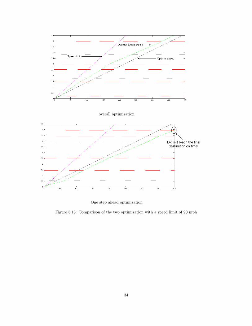
overall optimization
One step ahead optimization
Figure 5.13: Comparison of the two optimization with a speed limit of 90 mph
34

Chapter 6
Conclusions and future work
We developed a method using Dijkstra’s algorithm to determine the optimal path of a vehicle through a set
of traffic lights. The running time of this method depends on the number of nodes used to descretize the
problem. We saw that it could be greatly diminished by adequately choosing the positions of the nodes.
The analytical results for the one traffic light problem and the simulations for a realistic case suggested that
the optimal strategy was either to drive at the optimal speed or to hit the extremities of the traffic lights.
Consequently, we put nodes at the extremities of the red traffic lights (corners) and in the middle of the
green traffic light. By modifying the relations between nodes, we can perform different simulations: time
minimzation, fuel minimzation, one step ahead minimization, etc. Several opportunities for future research
on this topic could be based on this initial work. We highlight some of these in what follows.
6.1 Theoretical proofs
From our numerical calculations, the optimal strategy (given a fixed number of traffic lights with known
schedules) appears to be: either driving at the optimal speed or hitting the corners of the traffic lights.
Although we managed to obtain a proof of the suggested optimal strategy for simple cases, it remains to
show that it still holds for the general cases with many traffic lights.
6.2 Predictive control
In cases where the vehicle does not have all the information about the traffic lights, Dijkstra’s algorithm
cannot be used anymore and we can use one step ahead optimization (fuel minimization at each step).
When the final time is big enough, the one step ahead optimization and Dijkstra’s algorithm optimization
give similar results. However, if the final time is too small, the speed profile calculated can be inefficient
(we do not reach the destination on time). One could also consider n-steps ahead optimization, where n
(can be 1, 2, 3, etc) depends on the amount of information that we can obtain. An alternative could be to
35

perform the one step ahead optimization setting intermediate final times to make sure that one reaches the
final destination on time.
6.3 Traffic lights uncertainty
In this thesis, we assumed that the traffic light timing data had fixed values. An interesting problem would
be to take into account the uncertainty due to the traffic light timing, by considering time duration of the
red and green traffic lights as random variables with known statistics. To illustrate this idea, we can consider
the one traffic light problem shown in in Fig. 6.1. Here, tr is the expected value of the beginning of the red
traffic light and tr and tr are the extreme values of the actual time of the beginning of the red traffic light
(likewise for tg). It is the same kind of problem as in section 3.3 except that this time the constraints are
Figure 6.1: Uncertainity for the one traffic light problem
random variables. The problem to solve would be:
minV
f(V )
s.t gi(V ) ≤ 0 i = 1, 2, ..,m(6.1)
Here, f(V ) represents the expected value of the fuel consumption and gi(V ) are expectations with respect
to the random variables tr and tg. For more realistic situations, our Dijkstra’s algorithm method could be
adapted to take into account uncertainty by considering stochastic edge weights. The stochastic shortest
path problem has been studied a lot in the literature (e.g. [26],[27]) and could be investigated to be applied
to this kind of problem.
36

6.4 Improvement of fuel consumption model
6.4.1 Gear shifting
The objective of this thesis was to develop an algorithm which determines the optimal speed profile along a
trip using a simple model for the fuel consumption. A more accurate analysis should take into account the
effects of gear shifting and acceleration. For example, [1] proposed a model which takes into account gear
shifting and the effects of the brakes. However, if we assume a constant speed model between the traffic
lights, the effects of gear shifting can be negligible, contrary to the effects of the acceleration.
6.4.2 Acceleration
All the previous numerical analysis was done with steady state fuel model (no acceleration), but in the reality
the acceleration accounts for a significant amount of the total fuel consumption. Akcelik (1982) and Akcelik
and Bayley (1983) found an adequate model for the instantaneous fuel consumption [8]. It has the following
form:
F (V, a) =k1V
+ k2 + k3V2 + k4a+ k5a
2 (6.2)
In this formula,
• F is the instantaneous fuel consumption (mL/km)
• V is the instantaneous speed (km/hr)
• a is the instantaneous acceleration (km/hr2)
• k1 is the constant idling fuel consumption rate (mL/hr)
• k2 is the rolling resistance constant (mL/km)
• k3 is the air resistance constant (mL ∗ hr2/km3)
• k4 and k5 are the acceleration constants.
All these constants can be found experimentally and are obviously different for each vehicle. [8] gives the
values of these constants for their Melbourne University test car (Ford Cortina Wagon, 6-cylinder, 4.1L,
37

automatic transmission).
k1 k2 k3 k4 k5
2520 15.9 0.00792 0.00762 2.46 ∗ 10−7
For a = 0 (no acceleration), we can draw the consumption as a function of speed (Fig. 6.2) and we can see
that it has the same shape as Fig. 2.1.
Figure 6.2: Instantaneous fuel consumption with no acceleration
A simple numerical analysis permits to sense the impact of the acceleration terms. Let us consider a car
(with the same previous characteristics) which drives at 40 km/h during one kilometer and at 60 km/h during
another kilometer. If we do not take into account the acceleration terms the fuel consumption through this
trip is 178 mL (using formula 6.2). If we take into account the acceleration (assuming a uniform acceleration
in 10 seconds), the fuel consumption is 246 mL, which represents a 38% change.
6.4.3 Improvement of traffic model
Traffic light queuing is a complex topic and has been studied a lot in the literature (e.g. [30], [31]). A simple
way to take queuing and the flow of other vehicles into account would be to add constraints on the speed.
However, adding such constraints requires to know in advance the state of the traffic lights queues and of
the traffic flow.
38

References
[1] An F., Ross. M (1993) Model of Fuel Economy with Applications to Driving Cycles and Traffic Management
[2] An F., Ross. M (1993) A Model of Fuel Economy and Driving Patterns
[3] S. Boyd and L. Vandenberghe (2004) Convex Optimization, Cambridge University Press,
[4] Asadi, B.; Vahidi, A.; , ”Predictive Cruise Control: Utilizing Upcoming Traffic Signal Information for Improving FuelEconomy and Reducing Trip Time,” Control Systems Technology, IEEE Transactions on , vol.19, no.3, pp.707-714, May2011
[5] Christos H. Papadimitriou, Kenneth Steiglitz; , ”Combinatorial optimization : algorithms and complexity ” Mineola, N.Y.: Dover Publications, 1998
[6] ”Dijkstra’s algorithm.” Wikipedia, The Free Encyclopedia. Wikimedia Foundation, Inc.. 30 July 2012. Web. 2 Aug 2012.¡http://en.wikipedia.org/wiki/Dijkstra
[7] Ren, H. (2010, July 27). Lecture presented in The International Conference on Continuous Optimization. Santiago, Chile.¡http://www.cmm.uchile.cl/iccopt2010/renehenrion.pdf¿
[8] AKCELIK, R. (ED.) (1983). Progress in fuel consumption for urban Traffic Management. Research Report ARR 124.Australian Road Research Board, Vermont South, Australia.
[9] Beusen, B., Broekx, S., Denys, T., Beckx, C., Degraeuwe, B., Gijsbers, M., Scheepers, K., Govaerts, L., Torfs, R., andPanis, L. I. Using on-board logging devices to study the longer-term impact of an eco-driving course. Transpn Res. PartD, 2009, 14, 514520
[10] Li, S. E., and H. Peng. ”Strategies to Minimize the Fuel Consumption of Passenger Cars during Car-Following Scenarios.”Proceedings of the Institution of Mechanical Engineers, Part D: Journal of Automobile Engineering 226.3 (2012): 419-29.SCOPUS. Web. 23 Sep. 2012.
[11] Chang, D. J., Morlok, E. K. (2005). Vehicle Speed Profiles to Minimize Work and Fuel Consumption. Journal Of Trans-portation Engineering, 131(3), 173-182
[12] Bhm A, Jonsson M. Real-Time Communication Support for Cooperative, Infrastructure-Based Traffic Safety Applications.International Journal Of Vehicular Technology [serial online]. January 2011;2011:1-17.
[13] Maile, M., Ahmed-Zaid, F., Bai, S., Caminiti, L., Mudalige, P., Peredo, M., and Popovic, Z. (2011). Objective testing of acooperative intersection collision avoidance system for traffic signal and stop sign violation. Paper presented at the IEEEIntelligent Vehicles Symposium, Proceedings, 130-137
[14] M. Goralczyk, J. Pontow, F. Hausler, and I. Radusch, The automatic green light project - vehicular traffic optimizationvia velocity advice, in Adjunct Proceedings of the First International Conference on The Internet of Things, Zurich,Switzerland, 2008.
[15] A. Wegener, H. Hellbruck, C. Wewetzer, and A. Lubke, VANET simulation environment with feedback loop and itsapplication to traffic light assistance, in 2008 IEEE GLOBECOM Workshops, 2008.
[16] Li C, Shimamoto S. An Open Traffic Light Control Model for Reducing Vehicles’ CO2 Emissions Based on ETC Vehicles.IEEE Transactions On Vehicular Technology [serial online]. January 2012;61(1):97-110.
[17] U.S Department of Transportation, Washington, DC ”Intelligent Transportation Systems for Traffic Signal Control”.[online]. Available: http://ntl.bts.gov/lib/jpodocs/brochure/14321.htmb1
[18] Erik Hellstrm, Maria Ivarsson, Jan slund and Lars Nielsen, Look-ahead control for heavy trucks to minimize trip time andfuel consumption, 2009, Control Engineering Practice, (17), 2, 245-254.
[19] Maria Ivarsson.Fuel Optimal Powertrain Control for Heavy Trucks Utilizing Look Ahead. Thesis. Department of ElectricalEngineering Linkpings universitet, SE581 83 Linkping, Sweden Linkping 2009
[20] Lattemann, F., Neiss, K., Terwen, S., and Connolly, T., ”The Predictive Cruise Control A System to Reduce FuelConsumption of Heavy Duty Trucks,” SAE Technical Paper 2004-01-2616, 2004, doi:10.4271/2004-01-2616
[21] T. van Keulen, G. Naus, B. de Jager, R. van de Molengraft, M. Steinbuch, E. Aneke. Predictive Cruise Control in HybridElectric Vehicles. 2009. World Electric Vehicle Journal Vol. 3 - ISSN 2032-6653
39

[22] Li X, Yang H, Gao Z. Traffic control of urban corridor systems with weaving effects. Transportation Research: Part C[serial online].
[23] Kotsialos, A., Papageorgiou, M., Mangeas, M., Haj-Salem, H. (2002). Coordinated and integrated control of motorwaynetworks via non-linear optimal control. Transportation Research Part C: Emerging Technologies, 10(1), 65-84
[24] M. Bechler, J. Schiller, L. Wolf. In-car communication using wireless technology. [online]. Available: http ://134.169.34.11/users/bechler/myPublications/marcBeSW01.pdf
[25] M. S’anchez, J. C. Cano, D. Kim. 2006. Predicting Traffic lights to Improve Urban Traffic Fuel Consumption. 6th Inter-national Conference on ITS Telecommunications Proceedings
[26] Vladimirsky A. Label-Setting Methods for Multimode Stochastic Shortest Path Problems on Graphs. Mathematics OfOperations Research [serial online]. November 2008;33(4):821-838.
[27] Rinehart M, Dahleh M. The Value of Side Information in Shortest Path Optimization. IEEE Transactions On AutomaticControl [serial online]. September 2011;56(9):2038-2049.
[28] US Department of Energy. Transportation Energy Data Book: Chapter 4 light Vehicles and Characteristics. Available:http://cta.ornl.gov/data/chapter4.shtml
[29] ”Fuel economy vs speed 1997” Wikipedia, The Free Encyclopedia. Wikimedia Foundation, Inc.. 30 July 2012. Web. 01 Dec2012. < http : //en.wikipedia.org/wiki/F ile : Fueleconomyvsspeed1997.png >
[30] Bounds and Approximations for the Fixed-Cycle Traffic-Light Queue. Transportation Science [serial online]. November2006;40(4):484-496.
[31] Akgngr A, Bullen A. A New Delay Parameter for Variable Traffic Flows at Signalized Intersections. Turkish Journal OfEngineering and Environmental Sciences [serial online]. January 2007;31(1):61-70.
40