Ocean Modelling 30 (2009) 155–168

Contents lists available at ScienceDirect

Ocean Modelling

journal homepage: www.elsevier .com/locate /ocemod

CABARET in the ocean gyres

S.A. Karabasov a,d,*, P.S. Berloff b,c, V.M. Goloviznin d

a University of Cambridge, Department of Engineering, Whittle Laboratory, Cambridge, UKb Imperial College London, Grantham Institute for Climate Change and Department of Mathematics, London, UKc Woods Hole Oceanographic Institution, Physical Oceanography Department, Woods Hole, USAd Moscow Institute of Nuclear Safety of Russian Academy of Science, Moscow, Russia

a r t i c l e i n f o

Article history:Received 12 January 2009Received in revised form 18 June 2009Accepted 23 June 2009Available online 27 June 2009

Keywords:Mesoscale ocean dynamicsEddy resolving simulationsHigh-resolution schemes

1463-5003/$ - see front matter � 2009 Elsevier Ltd. Adoi:10.1016/j.ocemod.2009.06.009

* Corresponding author. Address: University ofEngineering, Whittle Laboratory, 1 JJ Thompson AvenTel.: +44 1223 337599.

E-mail address: sak36@eng.cam.ac.uk (S.A. Karaba

a b s t r a c t

A new high-resolution Eulerian numerical method is proposed for modelling quasigeostrophic oceandynamics in eddying regimes. The method is based on a novel, second-order non-dissipative and low-dis-persive conservative advection scheme called CABARET. The properties of the new method are comparedwith those of several high-resolution Eulerian methods for linear advection and gas dynamics. Then, theCABARET method is applied to the classical model of the double-gyre ocean circulation and its perfor-mance is contrasted against that of the common vorticity-preserving Arakawa method. In turbulentregimes, the new method permits credible numerical simulations on much coarser computational grids.

� 2009 Elsevier Ltd. All rights reserved.

1. Introduction

In many aspects mesoscale oceanic eddies, operating on thelengthscales of O(1–100) km are analogous to the cyclones andanticyclones that constitute the atmospheric weather phenome-non. The problem of resolving these eddies in a dynamically con-sistent way is very important for ocean modelling and, therefore,for global climate predictions. For achieving high Reynolds number(Re) simulations, which are required for accurate modelling of theocean, the models have to account for all important scales ofmotion.

Modern ocean models enter a new phase in which eddies willbe, at least, permitted in the numerical simulation. For such mod-els advection scheme is a very important component. A crucial ele-ment of numerical advection scheme is its ability to propagatefinite-amplitude and -phase disturbances on a discrete grid eitherwithout generating spurious short-wave oscillations, because ofnot preserving the correct dispersion relation i.e., dispersion error,or any considerable damping of the amplitude i.e., dissipation error(e.g., Kravchenko and Moin, 1997; Pope, 2000). Note, that the gen-eration of short-wave oscillations is particularly detrimental incase an inverse energy cascade takes place, and the small scales af-fect large scales (e.g., Tabeling, 2002; Vallis, 2006). In this paper,the effect of spurious small-scale dispersion and dissipation onimportant large-scale properties of the solution are captured by

ll rights reserved.

Cambridge, Department ofue, Cambridge CB3 0DY, UK.

sov).

comparing numerical predictions obtained with two differentadvection methods implemented within the same quasigeostroph-ic ocean modelling code (Berloff et al., 2007), which solves for theclassical double-gyre problem (Holland, 1978). The original modelimplements standard eddy viscosity for parameterising effects ofthe unresolved scales of turbulent diffusion and conservative sec-ond-order Arakawa scheme for advection (Arakawa, 1966). In thispaper, we consider a few versions of the original code based ondifferent advection methods. Comparisons with the convergedfine-grid solutions are made to investigate effects of numericaladvection schemes on the coarse-grid solutions.

Solving ‘convection-dominated’ problems is a longstandingchallenge for computational fluid dynamics (e.g., Rozhdestvenskyand Yanenko, 1978; Roache, 1982; Hirsch, 2007). One of the diffi-culties is that the conventional second-order finite-differenceschemes have large dispersion errors, which generate spurious rip-ples in the solutions. To counterbalance this effect, a numerical dis-sipation, such as the classical von Neumann and Richtmyer (1950)artificial viscosity for compression-type pressure waves or such asthe eddy viscosity in ocean circulation models, is added to the gov-erning equations. However, a common negative side of this ap-proach is the associated spurious dissipation that smears thelarge eddies along with the spurious ripples.

There are three general approaches for solving ‘convection-dominated’ problems: Eulerian, Lagrangian, and mixed Eulerian–Lagrangian. For the Eulerian methods, significant presence of bothnumerical dissipation and dispersion is common drawback. It ispartially overcome in the Lagrangian and Eulerian–Lagrangianmethods, which describe flow advection by following fluid particlecoordinates, rather than by considering fixed coordinates on the

156 S.A. Karabasov et al. / Ocean Modelling 30 (2009) 155–168

Eulerian grid (e.g., Dritschel et al., 1999; Mohebalhojeh and Drit-schel, 2004). A remarkable property of the Lagrangian methods isthat they are exact for the linear-advection problem with a uni-form velocity field, and in this case their accuracy is limited onlyby the accuracy of solving the corresponding Ordinary DifferentialEquations (ODEs), rather than by the accuracy of solving the fullPartial Differential Equations (PDEs), as in the Eulerian case. TheLagrangian methods can be very efficient for simulations with mul-tiple contact discontinuities and shocks, e.g., as those of multi-phase flows (e.g., Margolin and Shashkov, 2004). However, forthe problems dominated by chaotic folding and stretching of thematerial lines, the Lagrangian methods have to be complementedwith ad hoc ‘repair’ (or ‘contour surgery’) procedures. They allowto remove redundant Lagrangian particles that aggregate in somelocations and to add new particles to where they are needed. The‘repair’ procedure can be viewed as a special kind of numerical dis-sipation that drains energy from the underresolved scales. Thenumerical effect of the ‘repair’ procedure on the numerical dissipa-tion and dispersion error always limits Re for the resolved scales.Also, specifying standard physical boundary conditions (e.g.,no-slip, free-slip, etc.) is problematic for the Lagrangian methods.

The implementation of Eulerian–Lagrangian methods, includingsemi-Lagrangian and vortex-in-a-cell methods is less intricate,since they employ an Eulerian interpolation/projection step aftera Lagrangian step. However, they are no longer exact for the linearadvection, and they are prone to the same dissipation and disper-sion error problems as the Eulerian methods. For example, themixed Eulerian–Lagrangian methods use artificial numericaldissipation for avoiding the ‘repair’ procedure and for ensuring a‘non-oscillatory’ solution (e.g., Margolin, 1997). Finally, theLagrangian-to-Eulerian grid interpolation is also a source of thenumerical dissipation and dispersion errors.

Many Eulerian methods for ‘convection-dominated’ flows arebased on emphasizing a particular property of the governing equa-tions. Using such property as the basis for a ‘‘low-order” (first- orsecond-order) scheme, typically, further upgrades (e.g., high-order,non-oscillatory sequels, etc.) of the original scheme are developed.One such example is the family of optimised low-dispersion andlow-dissipation finite-difference schemes, including implicit com-pact finite-difference schemes based on Pade-type approximations(Lele, 1992) and explicit schemes (Tam and Webb, 1993; Bogeyand Bailly, 2004) that are popular in turbulence modelling. In par-ticular, the family of explicit schemes was developed to overcometypical problems of the spectral and pseudo-spectral methods,such as handling non-periodic boundary conditions and suitabilityfor parallel computations. The optimised explicit finite-differenceschemes, typically, employ non-conservative forms of the govern-ing equations, and use large computational stencils for more accu-rate approximation of the linear-wave dispersion relation in thephysical domain. In order to cope with the large unresolved gradi-ents emerging in nonlinear flows (e.g., shock waves) the high-orderlow-dissipative low-dispersive schemes use special filtering proce-dures (e.g., Robert, 1966; Asselin, 1972; Zhou and Wei, 2003). Suchfiltering is analogous to some form of artificial viscosity added tothe scheme and is required, essentially, to reduce the order ofthe scheme in the vicinity of the unresolved solution gradients,in accordance with the Godunov Theorem (Godunov, 1959), thatstates that any monotone finite-difference scheme is first-orderaccurate.

Another example consists of the so-called ‘‘high-resolutionschemes” (after A. Harten) that are based on Flux Corrected Trans-port (FCT), Total Variation Diminishing (TVD) solution ideas forquasi-linear hyperbolic conservation laws (e.g., Boris et al., 1975;Harten et al., 1987; LeVeque, 2002). In this approach a conservativeapproximation of the governing equations is used, that has severaluseful properties such as compact computational stencil, low CPU

cost, and, often, the solution boundness, but have large dissipationand/or dispersion errors. Then such schemes are upgraded to ahigher order, e.g., within the framework of ‘variable-extrapolation’and ‘flux-extrapolation’ techniques (e.g., van Leer, 1979; Wood-ward and Colella, 1984; Drikakis, 2003), by extending the spatialstencil. The upgrade is needed to enhance linear wave propagationproperties of the solution away from the flow discontinuities. Inthe vicinity of high-gradients of the solution, either nonlinear fluxlimiter (FCT/TVD) functions are used (Boris et al., 1975; Hartenet al., 1987; Pietrzak, 1998), or solution-adaptive stencils are used,as in WENO-type schemes (Shu and Osher, 1988). A significantimprovement of the linear wave propagation properties can alsobe obtained by introducing additional degrees of freedom insideeach computational cell, in the framework of Discontinuous Galer-kin methods (Cockburn and Shu, 2001), which are less sensitive tospatial grid non-uniformity, relative to the high-resolution finite-difference schemes.

Standard second- and third-order non-oscillatory schemes aretypically too dissipative for the problems in which the solution-front-sharpening mechanism is either absent or too weak to coun-terbalance the effect of the numerical dissipation. The higher costof implementation and the extra CPU cost of a high-order schemeis accepted by the computational community for some situations,when the conventional methods require prohibitively fine grids.One may argue that high-order discretisation in space is the onlyway to improve the solution, but we take a complimentary view.We argue that in a number of situations it is more efficient to im-prove the properties of the underlying discretisation by addressingadditional properties of the governing (hyperbolic) equations,within the class of second-order schemes. We argue that a hierar-chy of high-order schemes is better to be developed from a ‘‘low-order” method that is as accurate and efficient as possible. Thenthe order of the method can be systematically increased, consis-tently in space and time, and the low-dispersive and low-dissipativeproperties of the original scheme can be improved. Finally, becauseof their robustness, the second-order methods are still widely usedas a ‘‘working horse” in many hydrodynamics codes (e.g., for non-uniform grids, treatment of the shocks, ease with boundary condi-tions, etc.), and their improvement is important.

2. CABARET method

2.1. Linear advection scheme

To illustrate our ideas on a simple example, a scalar conserva-tion law

otuþ oxf ðuÞ ¼ 0 ð1Þ

is considered on a finite-difference grid which is non-uniform inspace xi+1 � xi = hi+1/2 and time tn+1 � tn = sn+1/2.

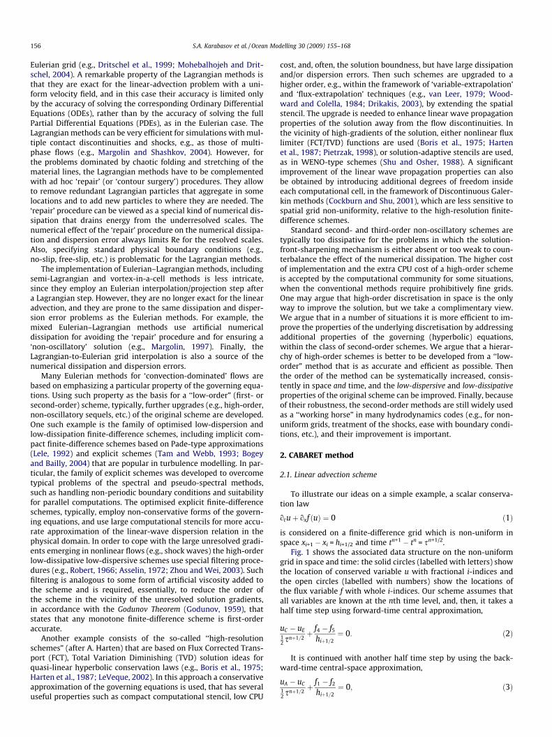
Fig. 1 shows the associated data structure on the non-uniformgrid in space and time: the solid circles (labelled with letters) showthe location of conserved variable u with fractional i-indices andthe open circles (labelled with numbers) show the locations ofthe flux variable f with whole i-indices. Our scheme assumes thatall variables are known at the nth time level, and, then, it takes ahalf time step using forward-time central approximation,

uC � uE12 snþ1=2

þ f4 � f5

hiþ1=2¼ 0: ð2Þ

It is continued with another half time step by using the back-ward-time central-space approximation,

uA � uC12 snþ1=2

þ f1 � f2

hiþ1=2¼ 0; ð3Þ

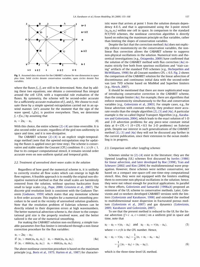
Fig. 1. Assumed data structure for the CABARET scheme for one dimension in spaceplus time. Solid circles denote conservation variables, open circles denote fluxvariables.

S.A. Karabasov et al. / Ocean Modelling 30 (2009) 155–168 157

where the fluxes f1, f2 are still to be determined. Note, that by add-ing these two equations, one obtains a conventional flux integralaround the cell 1254, with a trapezoidal rule evaluation of thefluxes. By symmetry, the scheme will be second-order accuratefor a sufficiently accurate evaluation of f1 and f2. We choose to eval-uate these by a simple upwind extrapolation carried out in an up-wind manner. Let’s assume for the moment that the sign of thewave speed, ouf(u), is positive everywhere. Then, we determinef1 = f(u1) by assuming that

u1 ¼ 2uC � u5: ð4Þ

With this choice, the entire scheme (2)–(4) are time-reversible. It isalso second order accurate, regardless of the gird non-uniformity inspace and time, and it is non-dissipative.

The CABARET scheme (2)–(4) is an explicit single-temporal-stage method (note that the upwind extrapolation step for updat-ing the fluxes is applied once per time step). The scheme is conser-vative and stable under the Courant (CFL) condition: 0 6 jcjs/h 6 1.Due to its compact computational stencil, it remains second orderaccurate even on non-uniform spatial and temporal grids.

2.2. Treatment of unresolved short-wave scales in the solution

Regardless of how good the numerical scheme is, it is unlikelyto correctly resolve all flow scales which can emerge in high-Reflow regimes. A feasible approach is to modify the original non-dis-sipative numerical method so that the small scales are harmlesslyremoved from the solution, without spurious backscatter fromsmall to large scales (e.g., Pope, 2000; Grinstein et al., 2007). Thediscrete grid resolution limit is consistent with the Godunov The-orem (Godunov, 1959) which states that any monotone schemeis first order accurate. This implies for a numerical smoothing pro-cedure to be used in the vicinity of unresolved solution gradients.Note that the resolution problem of Eulerian schemes can bedirectly related to their dispersion errors at high wavenumbers.The better numerical advection scheme is, the closer to the compu-tational grid size is the properly resolved wave, and the bettertailored is the use of the numerical smoothing.

For making the CABARET solution non-oscillatory, a simple tun-able-parameter-free flux limiter is introduced through a non-linearcorrection procedure for the flux variables:

u1 ¼ 2uC � u5;

if ðu1 > maxðu4; uE; u5ÞÞ u1 ¼maxðu4;uE;u5Þ;if ðu1 < minðu4;uE;u5ÞÞ u1 ¼minðu4;uE;u5Þ:

ð4aÞ

The above nonlinear correction procedure is based on the maximumprinciple (e.g., Boris et al., 1975; Harten et al., 1987) for character-

istic wave that arrives at point 1 from the solution domain depen-dency 4-E-5, and that is approximated using the 3-point stencil(u4,uE,u5) within one cell in space. In comparison to the standardFCT/TVD schemes, the nonlinear correction algorithm is directlybased on enforcing the maximum principle on flux variables, ratherthan limiting the slopes of conservation variables.

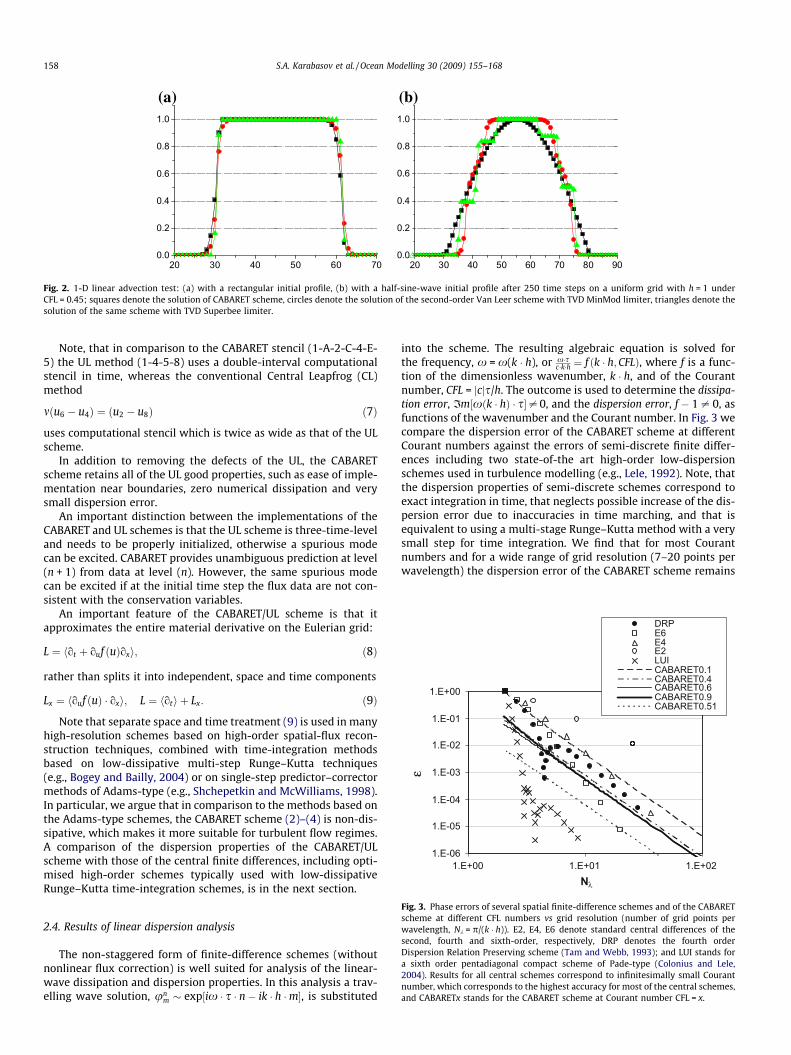
Despite the fact that the correction method (4a) does not explic-itly enforce monotonicity on the conservation variables, the non-linear flux correction allows the CABARET scheme to suppressnon-physical oscillations in the solution. Numerical tests and the-oretical investigations (e.g., Ostapenko, 2009) have confirmed thatthe solution of the CABARET method with flux correction (4a) re-mains strictly free both from spurious oscillations and ‘‘stair-cas-ing” artifacts of the standard TVD schemes (e.g., Shchepetkin andMcWilliams, 1998) for all Courant numbers CFL 6 0.5. Fig. 2 showsthe comparison of the CABARET solution for the linear advection ofdiscontinuous and continuous initial data with the second-ordervan Leer TVD scheme based on MinMod and Superbee limiters(e.g., Hirsch, 2007).

It should be mentioned that there are more sophisticated waysof introducing conservative correction in the CABARET scheme,than the simple limiter (4a). For example, there are algorithms thatenforce monotonicity simultaneously to the flux and conservationvariables (e.g., Goloviznin et al., 2003). For simple cases, e.g., forlinear advection with constant velocity, they produce more accu-rate results than the simple algorithm (2), (3) and (4a). A particularexample is the so-called Digital Transport Algorithm (e.g., Karaba-sov and Goloviznin, 2004), which leads to the exact solution of 1-Dand 2-D advection problems for any piece-wise constant initialdata at 0 < CFL < 1 (0 < CFL < 0.5 for 2-D problems) on Euleriangrids. Despite our interest in such generalizations of the CABARETmethod (2), (3) and (4a) they will not be discussed any further inthe current publication, since their extension to the ocean model-ling is in progress.

2.3. Comparison with other Leapfrog schemes

Schemes similar to (2)–(4) exist in the literature; they are theUpwind Leapfrog (UL) schemes first discussed by Iserles (1986)for linear advection, and later developed by Roe (1998), Tran andScheurer (2002) and Kim (2004) for multidimensional wave prop-agation. However, these schemes were neither conservative, norbased on a compact one-space-cell one-time-step computationalstencil. Also, they were not equipped with the limiters enablingthem to overcome non-physical oscillations in the solution; hence,they were not robust enough for practical applications. In parallelto these efforts, Goloviznin and Samarskii (1998a,b) proposed anextension of the UL scheme to conservative methods. Later, Golo-viznin and co-workers developed CABARET versions with the lim-iters (Goloviznin and Karabasov, 1998) and extended the methodto multidimensional wave dispersion in fracturated porous med-ium (Goloviznin et al., 2007) and gas dynamics (Goloviznin,2005; Karabasov and Goloviznin, 2007).

To see that the present method is reduced to the UL for the lin-ear advection (f = c � u, c = const.) on a uniform grid in space andtime, note that

uC � uE ¼ mðu5 � u4Þ and uE � uG ¼ mðu5 � u4Þ; ð5Þ

where m = cs/h is the CFL number. Hence,

uC � uE ¼ mðu5 � u4Þ ¼12

u1 þ u5 � u4 � u8ð Þ

¼ 12

u1 � u4ð Þ þ u5 � u8ð Þð Þ; ð6Þ

which is the three-time-level UL method.

1.E-06

1.E-05

1.E-04

1.E-03

1.E-02

1.E-01

1.E+00

1.E+00 1.E+01 1.E+02Nλ

ε

DRPE6E4E2LUICABARET0.1CABARET0.4CABARET0.6CABARET0.9CABARET0.51

20 30 40 50 60 700.0

0.2

0.4

0.6

0.8

1.0

20 30 40 50 60 70 80 900.0

0.2

0.4

0.6

0.8

1.0

(b) (a)

Fig. 2. 1-D linear advection test: (a) with a rectangular initial profile, (b) with a half-sine-wave initial profile after 250 time steps on a uniform grid with h = 1 underCFL = 0.45; squares denote the solution of CABARET scheme, circles denote the solution of the second-order Van Leer scheme with TVD MinMod limiter, triangles denote thesolution of the same scheme with TVD Superbee limiter.

158 S.A. Karabasov et al. / Ocean Modelling 30 (2009) 155–168

Note, that in comparison to the CABARET stencil (1-A-2-C-4-E-5) the UL method (1-4-5-8) uses a double-interval computationalstencil in time, whereas the conventional Central Leapfrog (CL)method

mðu6 � u4Þ ¼ ðu2 � u8Þ ð7Þ

uses computational stencil which is twice as wide as that of the ULscheme.

In addition to removing the defects of the UL, the CABARETscheme retains all of the UL good properties, such as ease of imple-mentation near boundaries, zero numerical dissipation and verysmall dispersion error.

An important distinction between the implementations of theCABARET and UL schemes is that the UL scheme is three-time-leveland needs to be properly initialized, otherwise a spurious modecan be excited. CABARET provides unambiguous prediction at level(n + 1) from data at level (n). However, the same spurious modecan be excited if at the initial time step the flux data are not con-sistent with the conservation variables.

An important feature of the CABARET/UL scheme is that itapproximates the entire material derivative on the Eulerian grid:

L ¼ ot þ ouf ðuÞoxh i; ð8Þ

rather than splits it into independent, space and time components

Lx ¼ ouf ðuÞ � oxh i; L ¼ oth i þ Lx: ð9Þ

Note that separate space and time treatment (9) is used in manyhigh-resolution schemes based on high-order spatial-flux recon-struction techniques, combined with time-integration methodsbased on low-dissipative multi-step Runge–Kutta techniques(e.g., Bogey and Bailly, 2004) or on single-step predictor–correctormethods of Adams-type (e.g., Shchepetkin and McWilliams, 1998).In particular, we argue that in comparison to the methods based onthe Adams-type schemes, the CABARET scheme (2)–(4) is non-dis-sipative, which makes it more suitable for turbulent flow regimes.A comparison of the dispersion properties of the CABARET/ULscheme with those of the central finite differences, including opti-mised high-order schemes typically used with low-dissipativeRunge–Kutta time-integration schemes, is in the next section.

Fig. 3. Phase errors of several spatial finite-difference schemes and of the CABARETscheme at different CFL numbers vs grid resolution (number of grid points perwavelength, Nk = p/(k � h)). E2, E4, E6 denote standard central differences of thesecond, fourth and sixth-order, respectively, DRP denotes the fourth orderDispersion Relation Preserving scheme (Tam and Webb, 1993); and LUI stands fora sixth order pentadiagonal compact scheme of Pade-type (Colonius and Lele,2004). Results for all central schemes correspond to infinitesimally small Courantnumber, which corresponds to the highest accuracy for most of the central schemes,and CABARETx stands for the CABARET scheme at Courant number CFL = x.

2.4. Results of linear dispersion analysis

The non-staggered form of finite-difference schemes (withoutnonlinear flux correction) is well suited for analysis of the linear-wave dissipation and dispersion properties. In this analysis a trav-elling wave solution, un

m � exp½ix � s � n� ik � h �m�, is substituted

into the scheme. The resulting algebraic equation is solved forthe frequency, x = x(k � h), or x�s

c�k�h ¼ f k � h;CFLð Þ, where f is a func-tion of the dimensionless wavenumber, k � h, and of the Courantnumber, CFL = jcjs/h. The outcome is used to determine the dissipa-tion error, Im½xðk � hÞ � s�– 0, and the dispersion error, f � 1 – 0, asfunctions of the wavenumber and the Courant number. In Fig. 3 wecompare the dispersion error of the CABARET scheme at differentCourant numbers against the errors of semi-discrete finite differ-ences including two state-of-the art high-order low-dispersionschemes used in turbulence modelling (e.g., Lele, 1992). Note, thatthe dispersion properties of semi-discrete schemes correspond toexact integration in time, that neglects possible increase of the dis-persion error due to inaccuracies in time marching, and that isequivalent to using a multi-stage Runge–Kutta method with a verysmall step for time integration. We find that for most Courantnumbers and for a wide range of grid resolution (7–20 points perwavelength) the dispersion error of the CABARET scheme remains

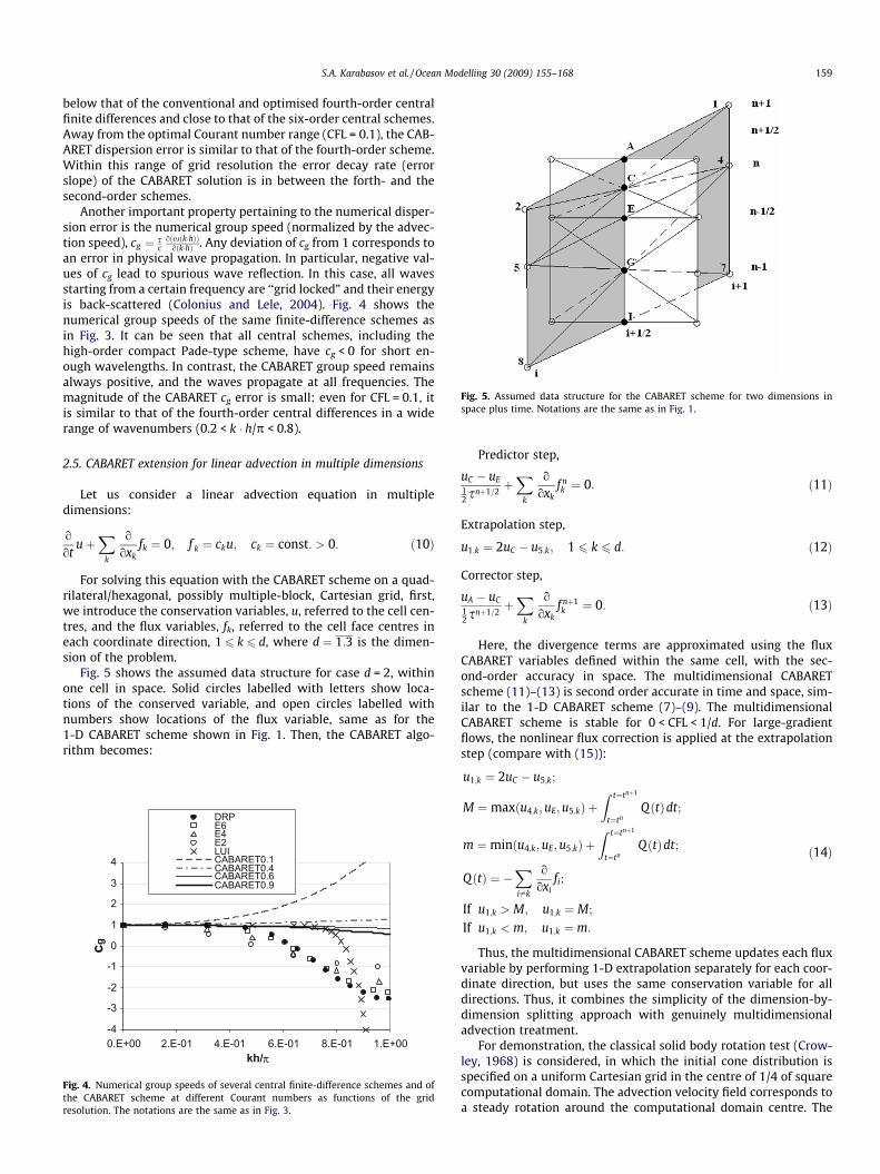
Fig. 5. Assumed data structure for the CABARET scheme for two dimensions inspace plus time. Notations are the same as in Fig. 1.

S.A. Karabasov et al. / Ocean Modelling 30 (2009) 155–168 159

below that of the conventional and optimised fourth-order centralfinite differences and close to that of the six-order central schemes.Away from the optimal Courant number range (CFL = 0.1), the CAB-ARET dispersion error is similar to that of the fourth-order scheme.Within this range of grid resolution the error decay rate (errorslope) of the CABARET solution is in between the forth- and thesecond-order schemes.

Another important property pertaining to the numerical disper-sion error is the numerical group speed (normalized by the advec-tion speed), cg ¼ s

co xðk�hÞð Þ

o k�hð Þ . Any deviation of cg from 1 corresponds toan error in physical wave propagation. In particular, negative val-ues of cg lead to spurious wave reflection. In this case, all wavesstarting from a certain frequency are ‘‘grid locked” and their energyis back-scattered (Colonius and Lele, 2004). Fig. 4 shows thenumerical group speeds of the same finite-difference schemes asin Fig. 3. It can be seen that all central schemes, including thehigh-order compact Pade-type scheme, have cg < 0 for short en-ough wavelengths. In contrast, the CABARET group speed remainsalways positive, and the waves propagate at all frequencies. Themagnitude of the CABARET cg error is small: even for CFL = 0.1, itis similar to that of the fourth-order central differences in a widerange of wavenumbers (0.2 < k � h/p < 0.8).

2.5. CABARET extension for linear advection in multiple dimensions

Let us consider a linear advection equation in multipledimensions:

o

otuþ

Xk

o

oxkfk ¼ 0; f k ¼ cku; ck ¼ const: > 0: ð10Þ

For solving this equation with the CABARET scheme on a quad-rilateral/hexagonal, possibly multiple-block, Cartesian grid, first,we introduce the conservation variables, u, referred to the cell cen-tres, and the flux variables, fk, referred to the cell face centres ineach coordinate direction, 1 6 k 6 d, where d ¼ 1:3 is the dimen-sion of the problem.

Fig. 5 shows the assumed data structure for case d = 2, withinone cell in space. Solid circles labelled with letters show loca-tions of the conserved variable, and open circles labelled withnumbers show locations of the flux variable, same as for the1-D CABARET scheme shown in Fig. 1. Then, the CABARET algo-rithm becomes:

-4

-3

-2

-1

0

1

2

3

4

0.E+00 2.E-01 4.E-01 6.E-01 8.E-01 1.E+00kh/π

c g

DRPE6E4E2LUICABARET0.1CABARET0.4CABARET0.6CABARET0.9

Fig. 4. Numerical group speeds of several central finite-difference schemes and ofthe CABARET scheme at different Courant numbers as functions of the gridresolution. The notations are the same as in Fig. 3.

Predictor step,

uC � uE12 snþ1=2

þX

k

o

oxkf nk ¼ 0: ð11Þ

Extrapolation step,

u1;k ¼ 2uC � u5;k; 1 6 k 6 d: ð12Þ

Corrector step,

uA � uC12 snþ1=2

þX

k

o

oxkf nþ1k ¼ 0: ð13Þ

Here, the divergence terms are approximated using the fluxCABARET variables defined within the same cell, with the sec-ond-order accuracy in space. The multidimensional CABARETscheme (11)–(13) is second order accurate in time and space, sim-ilar to the 1-D CABARET scheme (7)–(9). The multidimensionalCABARET scheme is stable for 0 < CFL < 1/d. For large-gradientflows, the nonlinear flux correction is applied at the extrapolationstep (compare with (15)):

u1;k ¼ 2uC � u5;k;

M ¼maxðu4;k;uE;u5;kÞ þZ t¼tnþ1

t¼tnQðtÞdt;

m ¼minðu4;k;uE;u5;kÞ þZ t¼tnþ1

t¼tnQðtÞdt;

QðtÞ ¼ �Xi–k

o

oxifi;

If u1;k > M; u1;k ¼ M;

If u1;k < m; u1;k ¼ m:

ð14Þ

Thus, the multidimensional CABARET scheme updates each fluxvariable by performing 1-D extrapolation separately for each coor-dinate direction, but uses the same conservation variable for alldirections. Thus, it combines the simplicity of the dimension-by-dimension splitting approach with genuinely multidimensionaladvection treatment.

For demonstration, the classical solid body rotation test (Crow-ley, 1968) is considered, in which the initial cone distribution isspecified on a uniform Cartesian grid in the centre of 1/4 of squarecomputational domain. The advection velocity field corresponds toa steady rotation around the computational domain centre. The

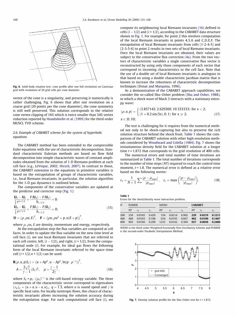
Fig. 6. Solid body rotation test: cone profile after one full revolution on Cartesiangrid with resolution of 20 grid cells per cone diameter.

Table 1Errors for the shock/density wave interaction problem.

N PLIMDE WENO CABARET

NT e1 ec NT e1 ec NT e1 ec

200 250 0.0185 0.429 334 0.0214 0.902 229 0.0219 0.1211400 468 0.0183 0.188 634 0.0195 0.667 462 0.0100 0.1467800 903 0.0166 0.290 1235 0.0162 0.369 927 0.0058 0.2400

WENO is the third-order Weighted Essentially Non-Oscillatory Scheme and PLIMDEis the second-order Parabolic Interpolation Method.

0

1

2

3

4

5

4 4.5 5 5.5 6 6.5 7 7.5 8x

ρρ

grid 400Converged

Fig. 7. Density solution profile for the Shu–Osher test for t = 1.872.

160 S.A. Karabasov et al. / Ocean Modelling 30 (2009) 155–168

vertex of the cone is a singularity, and preserving it numerically israther challenging. Fig. 6 shows that after one revolution on acoarse grid (20 points per the cone diameter), the cone symmetryis still well preserved. This solution corresponds to the relativecone vertex clipping of 16% which is twice smaller than 34% vertexreduction reported by Hundsdorfer et al. (1995) for the third-orderMUSCL TVD scheme.

2.6. Example of CABARET scheme for the system of hyperbolicequations

The CABARET method has been extended to the compressibleEuler equations with the use of characteristic decomposition. Stan-dard characteristic Eulerian methods are based on flow fielddecomposition into simple characteristic waves of constant ampli-tudes obtained from the solution of 1-D Riemann problem at eachcell face (e.g., LeVeque, 2002; Hirsch, 2007). In contrast to those,the CABARET extension to the equations in primitive variables isbased on the extrapolation of groups of characteristic variables,i.e., local Riemann invariants. In particular, the solution algorithmfor the 1-D gas dynamics is outlined below.

The components of the conservative variables are updated atthe predictor and corrector step (Fig. 1):

UC � UE12 snþ1=2

þ FðU4Þ � FðU5Þhiþ1=2

¼ 0;

UA � UC12 snþ1=2

þ FðU1Þ � FðU2Þhiþ1=2

¼ 0;

U ¼ ðq;qu; EÞT; F ¼ qu;qu2 þ p;uðEþ pÞ� �T

;

ð15Þ

where q, qu, E are density, momentum and energy, respectively.At the extrapolation step the flux variables are computed at cell

faces. In order to update the flux variable on the new time level atcell face (i), we use local Riemann invariants that are referred toeach cell centre, left, (i � 1/2), and right, (i + 1/2), from the compu-tational node (i). For example, for ideal gas flows the followingform of the local Riemann invariants referred to the space–timecell (i + 1/2,n + 1/2) can be used:

R q;u; p SCjð Þ ¼ uþ Apl;u� Apl

; lnðp � q�cÞ� �T

;

A ¼ 2ffiffifficp

c� 1SCð Þ

12c; l ¼ c� 1

2c; ð16Þ

where SC = pC � (qC)�c is the cell-based entropy variable. The threecomponents of the characteristic vector correspond to eigenvaluesfkqgC ¼ fuþ a;u� a;ugC ; q ¼ 1:3, where a is sound speed and c isspecific heat ratio. For locally isentropic flows, this choice of charac-teristic invariants allows increasing the solution accuracy duringthe extrapolation stage. For each computational cell face (i), we

compute its neighbouring local Riemann invariants (16) defined incells (i � 1/2) and (i + 1/2), according to the CABARET data structureshown in Fig. 1. For example, for point 2 this involves computationof the local Riemann invariants in points 4,5,6 and C,D,E,F. Theextrapolation of local Riemann invariants from cells (1-2-4-5) and(2-3-5-6) to point 2 results in two sets of local Riemann invariants.Once the local Riemann invariants are obtained, their values aresubject to the conservative flux correction (4a). From the two vec-tors of characteristic variables a single conservative flux vector isreconstructed by using only those components of each vector thatcorrespond to incoming characteristics to the cell face. Note thatthe use of a double set of local Riemann invariants is analogous tothat based on using a double characteristic Jacobian matrix that isknown to increase the robustness of characteristic decompositiontechniques (Donat and Marquina, 1996).

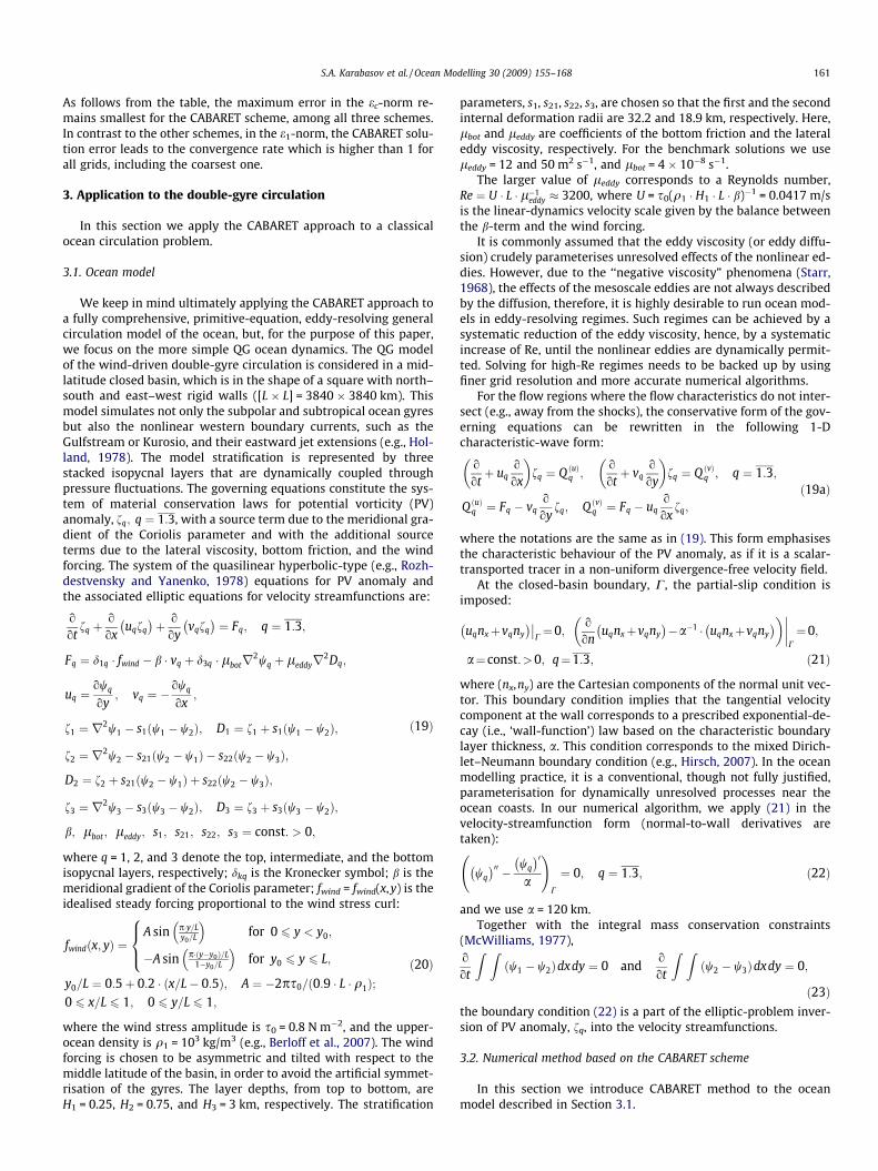
As a demonstration of the CABARET approach capabilities, weconsider the so-called Shu–Osher problem (Shu and Osher, 1988),in which a shock wave of Mach 3 interacts with a stationary entro-py wave:

ðq;u;pÞ ¼ð3:857143;2:629369;10:333333Þ for x < 2;

ð1þ 0:2 sinð5xÞ;0;1Þ for x P 2;

�x 2 ½0;10�:

ð17Þ

The test is challenging for it requires from the numerical meth-od not only to be shock-capturing but also to preserve the richsolution structure behind the shock front. Table 1 shows the com-parison of the CABARET solution with other high-resolution meth-ods considered by Woodward and Colella (1984). Fig. 7 shows theinstantaneous density field for the CABARET solution at a longertime t = 1.872 that corresponds to the grid resolution of 400 cells.

The numerical errors and total number of time iterations aresummarized in Table 1. The total number of iterations correspondsto the number of time steps (NT) required to reach the control timemoment, t = 1.8. The numerical error is defined as a relative errorbased on the following norms:

e1 ¼1

N þ 1

X q� qexactj jqexactj j ; ec ¼max

q� qexactj jqexactj j

� �: ð18Þ

S.A. Karabasov et al. / Ocean Modelling 30 (2009) 155–168 161

As follows from the table, the maximum error in the ec-norm re-mains smallest for the CABARET scheme, among all three schemes.In contrast to the other schemes, in the e1-norm, the CABARET solu-tion error leads to the convergence rate which is higher than 1 forall grids, including the coarsest one.

3. Application to the double-gyre circulation

In this section we apply the CABARET approach to a classicalocean circulation problem.

3.1. Ocean model

We keep in mind ultimately applying the CABARET approach toa fully comprehensive, primitive-equation, eddy-resolving generalcirculation model of the ocean, but, for the purpose of this paper,we focus on the more simple QG ocean dynamics. The QG modelof the wind-driven double-gyre circulation is considered in a mid-latitude closed basin, which is in the shape of a square with north–south and east–west rigid walls ([L � L] = 3840 � 3840 km). Thismodel simulates not only the subpolar and subtropical ocean gyresbut also the nonlinear western boundary currents, such as theGulfstream or Kurosio, and their eastward jet extensions (e.g., Hol-land, 1978). The model stratification is represented by threestacked isopycnal layers that are dynamically coupled throughpressure fluctuations. The governing equations constitute the sys-tem of material conservation laws for potential vorticity (PV)anomaly, fq; q ¼ 1:3, with a source term due to the meridional gra-dient of the Coriolis parameter and with the additional sourceterms due to the lateral viscosity, bottom friction, and the windforcing. The system of the quasilinear hyperbolic-type (e.g., Rozh-destvensky and Yanenko, 1978) equations for PV anomaly andthe associated elliptic equations for velocity streamfunctions are:

o

otfq þ

o

oxuqfq

� �þ o

oyvqfq

� �¼ Fq; q ¼ 1:3;

Fq ¼ d1q � fwind � b � vq þ d3q � lbotr2wq þ leddyr2Dq;

uq ¼owq

oy; vq ¼ �

owq

ox;

f1 ¼ r2w1 � s1 w1 � w2ð Þ; D1 ¼ f1 þ s1 w1 � w2ð Þ;

f2 ¼ r2w2 � s21 w2 � w1ð Þ � s22 w2 � w3ð Þ;

D2 ¼ f2 þ s21 w2 � w1ð Þ þ s22 w2 � w3ð Þ;

f3 ¼ r2w3 � s3 w3 � w2ð Þ; D3 ¼ f3 þ s3 w3 � w2ð Þ;

b; lbot; leddy; s1; s21; s22; s3 ¼ const: > 0;

ð19Þ

where q = 1, 2, and 3 denote the top, intermediate, and the bottomisopycnal layers, respectively; dkq is the Kronecker symbol; b is themeridional gradient of the Coriolis parameter; fwind = fwind(x,y) is theidealised steady forcing proportional to the wind stress curl:

fwindðx; yÞ ¼A sin p�y=L

y0=L

� for 0 6 y < y0;

�A sin p� y�y0ð Þ=L1�y0=L

� for y0 6 y 6 L;

8><>:

y0=L ¼ 0:5þ 0:2 � ðx=L� 0:5Þ; A ¼ �2ps0=ð0:9 � L � q1Þ;0 6 x=L 6 1; 0 6 y=L 6 1;

ð20Þ

where the wind stress amplitude is s0 = 0.8 N m�2, and the upper-ocean density is q1 = 103 kg/m3 (e.g., Berloff et al., 2007). The windforcing is chosen to be asymmetric and tilted with respect to themiddle latitude of the basin, in order to avoid the artificial symmet-risation of the gyres. The layer depths, from top to bottom, areH1 = 0.25, H2 = 0.75, and H3 = 3 km, respectively. The stratification

parameters, s1, s21, s22, s3, are chosen so that the first and the secondinternal deformation radii are 32.2 and 18.9 km, respectively. Here,lbot and leddy are coefficients of the bottom friction and the lateraleddy viscosity, respectively. For the benchmark solutions we useleddy = 12 and 50 m2 s�1, and lbot = 4 � 10�8 s�1.

The larger value of leddy corresponds to a Reynolds number,Re ¼ U � L � l�1

eddy � 3200, where U = s0(q1 � H1 � L � b)�1 = 0.0417 m/sis the linear-dynamics velocity scale given by the balance betweenthe b-term and the wind forcing.

It is commonly assumed that the eddy viscosity (or eddy diffu-sion) crudely parameterises unresolved effects of the nonlinear ed-dies. However, due to the ‘‘negative viscosity” phenomena (Starr,1968), the effects of the mesoscale eddies are not always describedby the diffusion, therefore, it is highly desirable to run ocean mod-els in eddy-resolving regimes. Such regimes can be achieved by asystematic reduction of the eddy viscosity, hence, by a systematicincrease of Re, until the nonlinear eddies are dynamically permit-ted. Solving for high-Re regimes needs to be backed up by usingfiner grid resolution and more accurate numerical algorithms.

For the flow regions where the flow characteristics do not inter-sect (e.g., away from the shocks), the conservative form of the gov-erning equations can be rewritten in the following 1-Dcharacteristic-wave form:

o

otþ uq

o

ox

� �fq ¼ Q ðuÞq ;

o

otþ vq

o

oy

� �fq ¼ Q ðvÞq ; q ¼ 1:3;

Q ðuÞq ¼ Fq � vqo

oyfq; Q ðvÞq ¼ Fq � uq

o

oxfq;

ð19aÞ

where the notations are the same as in (19). This form emphasisesthe characteristic behaviour of the PV anomaly, as if it is a scalar-transported tracer in a non-uniform divergence-free velocity field.

At the closed-basin boundary, C, the partial-slip condition isimposed:

uqnxþvqny� �

C¼0;

o

onuqnxþvqny� �

�a�1 � uqnxþvqny� �� �

C

¼0;

a¼ const:>0; q¼1:3; ð21Þ

where (nx,ny) are the Cartesian components of the normal unit vec-tor. This boundary condition implies that the tangential velocitycomponent at the wall corresponds to a prescribed exponential-de-cay (i.e., ‘wall-function’) law based on the characteristic boundarylayer thickness, a. This condition corresponds to the mixed Dirich-let–Neumann boundary condition (e.g., Hirsch, 2007). In the oceanmodelling practice, it is a conventional, though not fully justified,parameterisation for dynamically unresolved processes near theocean coasts. In our numerical algorithm, we apply (21) in thevelocity-streamfunction form (normal-to-wall derivatives aretaken):

wq

� �00 � wq

� �0a

!C

¼ 0; q ¼ 1:3; ð22Þ

and we use a = 120 km.Together with the integral mass conservation constraints

(McWilliams, 1977),o

ot

Z Zw1 � w2ð Þdxdy ¼ 0 and

o

ot

Z Zw2 � w3ð Þdxdy ¼ 0;

ð23Þthe boundary condition (22) is a part of the elliptic-problem inver-sion of PV anomaly, fq, into the velocity streamfunctions.

3.2. Numerical method based on the CABARET scheme

In this section we introduce CABARET method to the oceanmodel described in Section 3.1.

1 Note that without the flux corrections (35) and (36) the CABARET solution of the

162 S.A. Karabasov et al. / Ocean Modelling 30 (2009) 155–168

Let us consider a uniform Cartesian grid, xi+1,j � xi,j = h,yi,j+1 � yi,j = h, 1 6 i, j 6 N, which covers the entire computationaldomain. In addition to this grid, we consider the nodes staggeredfrom it by h/2:

xiþ1=2;jþ1=2 ¼ xi;j þ h=2; yiþ1=2;jþ1=2 ¼ yi;j þ h=2; ð24Þ

xi;jþ1=2 ¼ xi;j; yi;jþ1=2 ¼ yi;j þ h=2; ð25Þ

xiþ1=2;j ¼ xi;j þ h=2; yiþ1=2;j ¼ yi;j: ð26Þ

The conservation variables of the CABARET scheme are referred tothe cell centre points (fractional i and j indices); the flux variablesin the x-direction are referred to the cell face centres (whole i-indi-ces); and the flux variables in the y-direction are referred to the cellface centres (whole j-indices).

The extension of the 1-D CABARET algorithms (7)–(9) for theconservation law (19) is the following. At the predictor step, thePV anomaly value is computed at the mid-time level:

fq

� �nþ1=2iþ1=2;jþ1=2� fq

� �niþ1=2;jþ1=2

snþ1=2=2

þuq� �n

iþ1;jþ1=2 fq

� �niþ1;jþ1=2� uq

� �ni;jþ1=2 fq

� �ni;jþ1=2

h

þvq� �n

iþ1=2;jþ1 fq

� �niþ1=2;jþ1� vq

� �niþ1=2;j fq

� �niþ1=2;j

h¼ Fq� �nþ1=2

iþ1=2;jþ1=2; q¼1:3; ð27Þ

where ðFqÞnþ1=2iþ1=2;jþ1=2 denotes the second-order accurate approxima-

tion (discussed later in this section) of the source function at themid-time level; and the minimal local step, according to the stabil-ity constraint, is

snþ1=2 ¼ min16i;j6N

CFL � h=max uq� �n

i;jþ1=2

; vq� �n

iþ1=2;j

� h i; ð28Þ

where 0 < CFL < 0.5. The updated values of PV anomaly are used tocompute the mid-time-level velocity streamfunction and its Lapla-cian, by solving the system of the elliptic equations,

f1ð Þnþ1=2iþ1=2;jþ1=2 ¼ r

2w1

� nþ1=2

iþ1=2;jþ1=2� s1 w1ð Þ

nþ1=2iþ1=2;jþ1=2� w2ð Þ

nþ1=2iþ1=2;jþ1=2

� ;

f2ð Þnþ1=2iþ1=2;jþ1=2 ¼ r

2w2

� nþ1=2

iþ1=2;jþ1=2� s21 w2ð Þ

nþ1=2iþ1=2;jþ1=2� w1ð Þ

nþ1=2iþ1=2;jþ1=2

� � s22 w2ð Þ

nþ1=2iþ1=2;jþ1=2� w3ð Þ

nþ1=2iþ1=2;jþ1=2

� ;

f3ð Þnþ1=2iþ1=2;jþ1=2 ¼ r

2w3

� nþ1=2

iþ1=2;jþ1=2� s3 w3ð Þ

nþ1=2iþ1=2;jþ1=2� w2ð Þ

nþ1=2iþ1=2;jþ1=2

� ;

ð29Þ

complemented by the partial-slip boundary condition (22) approx-imated with the second-order one-sided finite-differences and bythe imposed mass conservation constraint (23).

Once ðwqÞnþ1=2iþ1=2;jþ1=2 is calculated, it is used for updating the veloc-

ity components at the cell faces:

wq

� �nþ1=2

i;j¼1

4wq

� �nþ1=2

iþ1=2;jþ1=2þ wq

� �nþ1=2

iþ1=2;j�1=2þ wq

� �nþ1=2

i�1=2;jþ1=2

�þ wq

� �nþ1=2

i�1=2;j�1=2

;

uq� �nþ1=2

i;jþ1=2 ¼wq

� �nþ1=2

i;jþ1� wq

� �nþ1=2

i;j

h;

vq� �nþ1=2

iþ1=2;j ¼ �wq

� �nþ1=2

iþ1;j� wq

� �nþ1=2

i;j

h: ð30Þ

Then, each velocity component is extrapolated to the new timelevel, n + 1, with the second-order accuracy:

uq� �nþ1

i;jþ1=2 ¼ ð1þ dÞ uq� �nþ1=2

i;jþ1=2 � d uq� �n�1=2

i;jþ1=2;

vq� �nþ1

i;jþ1=2 ¼ ð1þ dÞ vq� �nþ1=2

i;jþ1=2 � d vq� �n�1=2

i;jþ1=2;

d ¼ snþ1=2

snþ1=2 þ sn�1=2 :

ð31Þ

Once the velocity field is updated, the extrapolation step yields thenew values of the flux variables:

fq

� �nþ1iþ1;jþ1=2¼2 fq

� �nþ1=2iþ1=2;jþ1=2� fq

� �ni;jþ1=2 if uq

� �nþ1iþ1;jþ1=2 P0;

fq

� �nþ1i;jþ1=2¼2 fq

� �nþ1=2iþ1=2;jþ1=2� fq

� �niþ1;jþ1=2 if uq

� �nþ1i;jþ1=2<0;

ð32Þ

and

fq

� �nþ1iþ1=2;jþ1 ¼ 2 fq

� �nþ1=2iþ1=2;jþ1=2 � fq

� �niþ1=2;j if vq

� �nþ1iþ1=2;jþ1 P 0;

fq

� �nþ1iþ1=2;j ¼ 2 fq

� �nþ1=2iþ1=2;jþ1=2 � fq

� �niþ1=2;jþ1 if vq

� �nþ1iþ1=2;j < 0:

ð33Þ

At the lateral boundary cells, the upstream cell-face values are notavailable, because the partial-slip boundary condition is imposed onthe corresponding centre-cell variables. Therefore, we use the first-order upwind approximation, e.g.:

fq

� �nþ11;jþ1=2 ¼ fq

� �nþ1=21=2;jþ1=2 if uq

� �nþ11;jþ1=2 P 0: ð34Þ

The computed cell-face values of the PV anomaly are corrected,1 ifthey are outside the limits given by the maximum principle:

If fq

� �nþ1i;jþ1=2 > Mq

� �nþ1i;jþ1=2; fq

� �nþ1i;jþ1=2 ¼ Mq

� �nþ1i;jþ1=2;

If fq

� �nþ1i;jþ1=2 < mq

� �nþ1i;jþ1=2; fq

� �nþ1i;jþ1=2 ¼ mq

� �nþ1i;jþ1=2;

ð35Þ

and

If fq

� �nþ1iþ1=2;j > Mq

� �nþ1iþ1=2;j; fq

� �nþ1iþ1=2;j ¼ Mq

� �nþ1iþ1=2;j;

If fq

� �nþ1iþ1=2;j < mq

� �nþ1iþ1=2;j; fq

� �nþ1iþ1=2;j ¼ mq

� �nþ1iþ1=2;j:

ð36Þ

Here, the minimum and maximum limit values account not only forthe solution at the previous time step, as in (15), but also for thenon-zero right-hand side in (19a). Thus, for a cell facing in thex-direction, we have:

If uq� �nþ1

iþ1;jþ1=2 P 0

Mq� �nþ1

iþ1;jþ1=2 ¼max fq

� �ni;jþ1=2; fq

� �niþ1=2;jþ1=2; fq

� �niþ1;jþ1=2

� þ Q ðuÞq

� n

iþ1=2;jþ1=2�snþ1=2;

mq� �nþ1

iþ1;jþ1=2 ¼min fq

� �ni;jþ1=2; fq

� �niþ1=2;jþ1=2; fq

� �niþ1;jþ1=2

� þ Q ðuÞq

� n

iþ1=2;jþ1=2�snþ1=2;

8>>>>>>>>><>>>>>>>>>:

ð37Þ

and

If uq� �nþ1

i;jþ1=2 < 0

Mq� �nþ1

i;jþ1=2¼max fq

� �ni;jþ1=2; fq

� �niþ1=2;jþ1=2; fq

� �niþ1;jþ1=2

� þ Q ðuÞq

� n

iþ1=2;jþ1=2�snþ1=2;

mq� �nþ1

i;jþ1=2 ¼min fq

� �ni;jþ1=2; fq

� �niþ1=2;jþ1=2; fq

� �niþ1;jþ1=2

� þ Q ðuÞq

� n

iþ1=2;jþ1=2�snþ1=2;

8>>>>>>>>><>>>>>>>>>:

ð38Þ

double-gyre problem diverges, same as the Arakawa method without the Robert–Asselin filtering in time.

S.A. Karabasov et al. / Ocean Modelling 30 (2009) 155–168 163

where the source term is evaluated by approximating (19a) withthe first-order accuracy in time and with the second-order accuracyin space:

Q q

� �nþ1=2iþ1=2;jþ1=2 ¼

fq

� �nþ1=2iþ1=2;jþ1=2 � fq

� �niþ1=2;jþ1=2

snþ1=2=2

þ uq� �

iþ1=2;jþ1=2

fq

� �niþ1;jþ1=2 � fq

� �ni;jþ1=2

h: ð39Þ

Here, uq� �

iþ1=2;jþ1=2 ¼12 uq� �nþ1

iþ1;jþ1=2 þ uq� �nþ1

i;jþ1=2

� in the domain inte-

rior, and (uq)i+1/2,j+1/2 = 0 on the boundary. In (39), the first-orderaccuracy in time cannot affect the overall order of accuracy of thealgorithm, because approximation (39) is used only in the non-dif-ferential constraint (36).

Once the flux variables are updated at the new time step, thenew values of the centre-cell conservation variables are computedat the corrector step:

fq

� �nþ1iþ1=2;jþ1=2� fq

� �nþ1=2iþ1=2;jþ1=2

snþ1=2=2

þuq� �nþ1

iþ1;jþ1=2 fq

� �nþ1iþ1;jþ1=2� uq

� �nþ1i;jþ1=2 fq

� �nþ1i;jþ1=2

h

þvq� �nþ1

iþ1=2;jþ1 fq

� �nþ1iþ1=2;jþ1� vq

� �nþ1iþ1=2;j fq

� �nþ1iþ1=2;j

h¼ Fq� �nþ1=2

iþ1=2;jþ1=2; q¼1:3:

ð40Þ

For well-resolved solution regions, where the corrections (34) and(35) remain inactive, the CABARET scheme (27)–(40) approximatesthe conservation laws (19) to the second order of accuracy in bothspace and time, provided that the approximation of the full source

term, ðFqÞnþ1=2iþ1=2;jþ1=2, is second-order accurate.

In our algorithm, the full source term is separated into the com-bined wind and viscous component and into the b-termcomponent:

Fq� �nþ1=2

iþ1=2;jþ1=2 ¼ Fviscþwindq

� nþ1=2

iþ1=2;jþ1=2þ FCoriolis

q

� nþ1=2

iþ1=2;jþ1=2: ð41Þ

We find that in the ocean simulations the b-term component isnumerically stiff, and, therefore, it can excite spurious basin-scalebarotropic modes. In order to avoid this problem, a separate secondorder accurate predictor–corrector Adams-type scheme is used inorder to increase the stability of the approximation in time:

FCoriolisq

� nþ1=2

iþ1=2;jþ1=2¼ ð1þ dÞ Rq

� �niþ1=2;jþ1=2 � d Rq

� �n�1iþ1=2;jþ1=2;

d ¼ snþ1=2

2sn�1=2 ; ð42Þ

where the residual is

Rq� �n

iþ1=2;jþ1=2 ¼ �12

b vq� �n

iþ1=2;jþ1 þ vq� �n

iþ1=2;j

� : ð43Þ

In our numerical algorithm, the b-term component (42) is added tothe equations at the predictor time step (27).

Since, unlike in the Arakawa method, in the absence of viscousforces our method is equivalent to the conservation law of PVanomaly plus the b-term, rather than to the conservation law ofPV itself,

R Rðfq þ b � yÞdxdy ¼ const:; q ¼ 1:3, we need to make

sure that our scheme is compatible with the discrete PV conserva-tion law. This is indeed the case, since (43) is equivalent to the fol-lowing conservative approximation of the b-term component:

Rq� �n

iþ1=2;jþ1=2 ¼ Fluxjþ1 � Fluxj þ Fluxiþ1 � Fluxi þ OðdivÞ;

Fluxj ¼ �byj vq� �n

iþ1=2;j

.h; Fluxi ¼ �byjþ1=2 uq

� �ni;jþ1=2

.h;

yjþ1=2 ¼12

yjþ1 þ yj

� �;

ð43aÞ

and OðdivÞ ¼ byjþ1=2ðuqÞniþ1;jþ1=2�ðuqÞni;jþ1=2

h þ ðvqÞniþ1=2;jþ1�ðvqÞniþ1=2;j

h

h i¼ 0, because

the velocity field obtained from (29) and (30) is divergence-free. Wehave checked that the velocity divergence term is indeed of the or-der of round off error in all our calculations.

In contrast to the b-term component, the other component ofthe source term is numerically benign, and, therefore, it is approx-imated at the mid-time level by the second-order differences ofboth the velocity streamfunction and its Laplacian. The corre-sponding term is added to the equations after the elliptic problem(29) is solved, and after the velocity streamfunction at the mid-time level is updated:

Fviscþwindq

� nþ1=2

iþ1=2;jþ1=2¼ d1q � fwind þ d3q � lbot r2wq

� nþ1=2

iþ1=2;jþ1=2

þ lvol r2Dq

� nþ1=2

iþ1=2;jþ1=2: ð44Þ

Here, the Laplacians are evaluated directly from the solution ofelliptic problems at the mid-time level:

r2w1

� nþ1=2

iþ1=2;jþ1=2¼ f1ð Þnþ1=2

iþ1=2;jþ1=2þ s1 w1ð Þnþ1=2iþ1=2;jþ1=2� w2ð Þ

nþ1=2iþ1=2;jþ1=2

� ;

r2w2

� nþ1=2

iþ1=2;jþ1=2¼ f2ð Þnþ1=2

iþ1=2;jþ1=2þ s21 w2ð Þnþ1=2iþ1=2;jþ1=2� w1ð Þ

nþ1=2iþ1=2;jþ1=2

� þ s22 w2ð Þ

nþ1=2iþ1=2;jþ1=2� w3ð Þ

nþ1=2iþ1=2;jþ1=2

� ;

r2w3

� nþ1=2

iþ1=2;jþ1=2¼ f3ð Þnþ1=2

iþ1=2;jþ1=2þ s3 w3ð Þnþ1=2iþ1=2;jþ1=2� w2ð Þ

nþ1=2iþ1=2;jþ1=2

� :

ð45Þ

In order to untangle the variables in the elliptical problem (45),the vertical normal-mode variables are employed. They allow todiagonalise the elliptic problem into the three independent Helm-holtz problems (for the individual vertical modes), that are solvedwith the combined Fast Fourier Transform (FFT) and cyclic reduc-tion methods.

4. Ocean modelling results

In this section, we discuss the ocean circulation solutions ob-tained with the CABARET algorithm and compare the results withthose obtained by using the conventional second-order Arakawamethod. The Arakawa method is based on the CL advection schemeand Robert–Asselin filtering in time (with the relaxation constantequal to 0.1). We have actually checked that the results reportedin this section for the Arakawa method are virtually insensitiveto the relaxation constant in the range 0.01–0.3. Both methodsare implemented in the same quasigeostrophic ocean modellingcode that (with the Arakawa method) was previously used in dou-ble-gyre simulations (e.g., Berloff et al., 2007). We also checkedthat, in comparison with the conventional Arakawa method, theCABARET method (24)–(42) is about 1.2–2 times slower. However,this is a small drawback relative to the advantage of the greatly in-creased accuracy of the model.

4.1. Moderate Reynolds numbers

First, we compare the CABARET method with the conventionalsecond-order method and with a low-dispersion first-order up-wind method. We use leddy = 50 m2 s�1 that corresponds to a mod-erate-Re flow regime, Re = 3200. We use four uniform Cartesiangrids with 129 � 129, 257 � 257, 513 � 513, and 1025 � 1025nodes. For the moderate-Re case the solution convergence is con-firmed against the finest grid, 2059 � 2059 simulation, which is al-most indistinguishable from the fine 1025-grid solution (e.g., thedifference of maximum r.m.s. fluctuations of the eastward jet isless than 0.1%). Each simulation starts from the state of rest, and

164 S.A. Karabasov et al. / Ocean Modelling 30 (2009) 155–168

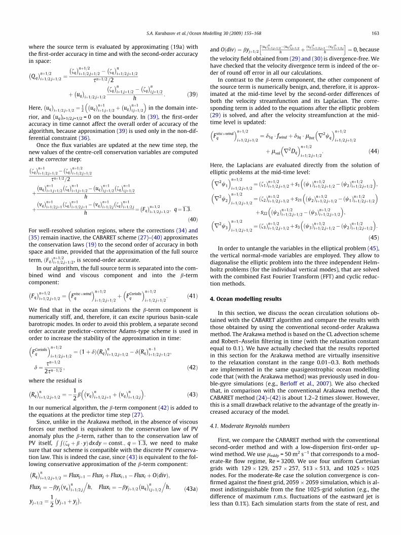
each physical run time is 104 days, which corresponds to about0.5–1 million time steps on the fine, 10252 grid. The spin-up time,during which all solutions reach statistically stationary states, is8000 days. The data for further processing are stored for theremaining physical time of 2000 days, which is long relative tomost of the characteristic time scales of the mesoscale eddies.For the purpose of the grid convergence study, we consider thetime averages of the solutions and their r.m.s. fluctuations. At themoderate Re = 3200, the Arakawa scheme begins to converge start-ing from the 513-grid (Figs. 8 and 9). On the 257-grid, the westernboundary current eastward jet (EJ) separates below the correct lat-itude (as given by the converged finest-grid solution). We suggestthat this spurious behaviour of the EJ is an artifact of the numericaldissipation and dispersion errors that can be significantly correctedwith the CABARET algorithm. Overall, correct modelling of the EJ isone of the key targets that we seek to achieve on relatively coarsegrids.

The convergence of the CABARET and Arakawa methods havebeen checked in three error norms and by the location of the sep-aration point of the jet on the EJ (Table 2). The first two errors cor-respond to the standard maximum norm of the time-averagedupper-ocean streamfunction solution and to that of the r.m.s. fluc-tuations of the upper-ocean streamfunction solution, respectively.The third error corresponds to the absolute value of the relative er-ror in predicting the maximum of the r.m.s. fluctuations of theupper-ocean streamfunction solution that characterises thestrength of the EJ. As seen from the table, the CABARET schemeshows significantly smaller errors and faster convergence rate forall error norms in comparison to the Arakawa scheme, which formax ew1

�� �� norm even fails to converge. The CABARET convergence

Fig. 8. Convergence of the Arakawa and CABARET methods for the moderate-Re case. Tim513 � 513 grid, and (c) 1025 � 1025 grid.

rate is approximately linear in the maximum norms. For bothmethods, the relative error of the maximum r.m.s. jet fluctuationsdecays faster than the quadratic rate, with the CABARETmethod being still superior. The convergence of the EJ separationpoint is in Table 3, and it also shows a superiority of the CABARETsolution.

4.2. High Reynolds numbers

The advantages of the CABARET method over the conventionalsecond-order methods are more pronounced at high Re. To demon-strate this, we computed the double-gyre problem for a largeRe � 13,300 (leddy = 12 m2 s�1).

With our grid resolutions, and, unlike in the moderate-Re case(Section 4.1), there is no evidence of the solution convergence foreither of the schemes except for the jet separation point locationon the western boundary (Table 4).

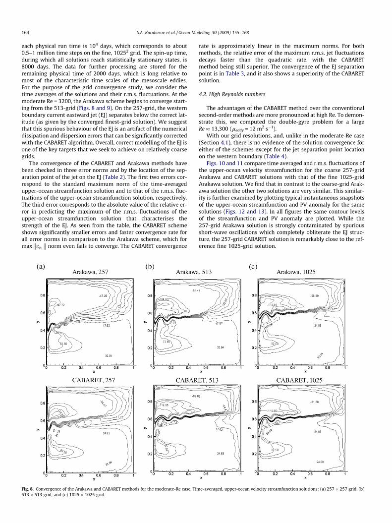
Figs. 10 and 11 compare time averaged and r.m.s. fluctuations ofthe upper-ocean velocity streamfunction for the coarse 257-gridArakawa and CABARET solutions with that of the fine 1025-gridArakawa solution. We find that in contrast to the coarse-grid Arak-awa solution the other two solutions are very similar. This similar-ity is further examined by plotting typical instantaneous snapshotsof the upper-ocean streamfunction and PV anomaly for the samesolutions (Figs. 12 and 13). In all figures the same contour levelsof the streamfunction and PV anomaly are plotted. While the257-grid Arakawa solution is strongly contaminated by spuriousshort-wave oscillations which completely obliterate the EJ struc-ture, the 257-grid CABARET solution is remarkably close to the ref-erence fine 1025-grid solution.

e-averaged, upper-ocean velocity streamfunction solutions: (a) 257 � 257 grid, (b)

Fig. 9. Convergence of the Arakawa and CABARET methods for the moderate-Re case. The r.m.s. fluctuation of upper-ocean velocity streamfunction solutions: (a) 257 � 257grid, (b) 513 � 513 grid, and (c) 1025 � 1025 grid.

Table 2Error convergence for the moderate-Re case.

Grid CABARET Arakawa CABARET Arakawa CABARET Arakawa

max ew1

�� �� max ew1

�� �� max er:m:s:ðw1Þ�� �� max er:m:s:ðw1Þ

�� �� ekmax(r.m.s.(w1))k ekmax(r.m.s.(w1))k

129 142.22 138.48 99.39 104.25 0.47 0.315257 132.66 189.07 56.58 86.87 0.071 0.098513 50.98 199.44 34.42 71.29 0.003 0.012

Table 3Convergence of the location of the separation point, y/L.

Grid 257 513 1025

Arakawa 0.4 0.5 0.55CABARET 0.5 0.55 0.55

The confidence interval for the error in separation point location, which was esti-mated by graphical data post-processing in Tecplot, is about ±0.01.

Table 4Location of the separation point, y/L.

Grid 257 513 1025

Arakawa N/A 0.3 0.5CABARET 0.5 0.55 0.5

See the footnotes of Table 3.

S.A. Karabasov et al. / Ocean Modelling 30 (2009) 155–168 165

To further validate this qualitative picture, we have checkedthat the underprediction of the maximum r.m.s. fluctuations ofthe EJ of the 257-grid Arakawa solution, in comparison to the ref-

erence 1025 solution, is 65%, thus indicating a total failure of thesolution. In contrast to this, the CABARET solution on the 257 gridresults in only 19% error in the maximum r.m.s. fluctuations of theEJ. We find this qualitative agreement with the 1025-grid solutionremarkable, given that computation with the coarse 257-grid CAB-ARET is more than 30 times faster than that with the fine 1025-gridArakawa scheme.

5. Conclusions and discussion

The novel Compact Accurately Boundary Adjusting high-REso-lution Technique (CABARET) works remarkably well for the eddy-resolving quasigeostrophic double-gyre ocean circulation problem.In comparison with the conventional second-order method, it al-lows to increase Reynolds number (Re) of the simulations by an or-der of magnitude - this opens exciting perspectives for exploringmore realistic flow regimes.

The CABARET approach is based on several important ideas,which have been circulating in the computational physicscommunity:

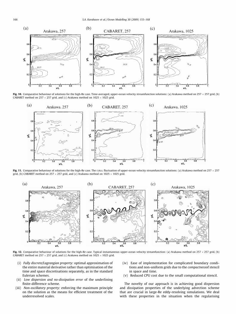
Fig. 10. Comparative behaviour of solutions for the high-Re case. Time-averaged, upper-ocean velocity streamfunction solutions: (a) Arakawa method on 257 � 257 grid, (b)CABARET method on 257 � 257 grid, and (c) Arakawa method on 1025 � 1025 grid.

Fig. 11. Comparative behaviour of solutions for the high-Re case. The r.m.s. fluctuation of upper-ocean velocity streamfunction solutions: (a) Arakawa method on 257 � 257grid, (b) CABARET method on 257 � 257 grid, and (c) Arakawa method on 1025 � 1025 grid.

Fig. 12. Comparative behaviour of solutions for the high-Re case. Typical instantaneous upper-ocean velocity streamfunction: (a) Arakawa method on 257 � 257 grid, (b)CABARET method on 257 � 257 grid, and (c) Arakawa method on 1025 � 1025 grid.

166 S.A. Karabasov et al. / Ocean Modelling 30 (2009) 155–168

(i) Fully discrete/Lagrangian property: optimal approximation ofthe entire material derivative rather than optimisation of thetime and space discretisations separately, as in the standardEulerian schemes.

(ii) Low dispersion and no-dissipation error of the underliningfinite-difference scheme.

(iii) Non-oscillatory property: enforcing the maximum principleon the solution as the means for efficient treatment of theunderresolved scales.

(iv) Ease of implementation for complicated boundary condi-tions and non-uniform grids due to the compactnessof stencilin space and time.

(v) Reduced CPU cost due to the small computational stencil.

The novelty of our approach is in achieving good dispersionand dissipation properties of the underlying advection schemethat are crucial in large-Re eddy-resolving simulations. We dealwith these properties in the situation when the regularising

Fig. 13. Comparative behaviour of solutions for the high-Re case. Typical instantaneous upper-ocean PV anomaly: (a) Arakawa method on 257 � 257 grid, (b) CABARETmethod on 257 � 257 grid, and (c) Arakawa method on 1025 � 1025 grid.

S.A. Karabasov et al. / Ocean Modelling 30 (2009) 155–168 167

effect of the explicit eddy viscosity is small relative to the dissi-pation and dispersion errors of the scheme. In order to prove thispoint, we presented a systematic comparison of the new CABA-RET method with popular high-resolution methods such as MUS-CL, PPM and WENO, for several linear-advection and gasdynamics problems. Finally, we contrasted the performance ofthe CABARET scheme with that of the standard second-orderArakawa method for the classical ocean circulation problem. Inparticular we show that the numerical dispersion and dissipationerror of the latter can be responsible for largely incorrect east-ward jet structure.

For the double-gyre circulation, the CABARET method allowsone to obtain high-quality solutions on the grid that has half apoint over the Munk lengthscale, (leddy/b)1/3, which characterisesthe viscous western boundary layer. This is a very significant up-grade relative to the conventional scheme that requires 2–3 gridpoints over this lengthscale (e.g., Berloff et al., 2007).

In the current publication we have not attempted to implementother high-resolution schemes, such as those quoted in Section 2,for the double-gyre problem and to compare them with the CABA-RET method. This is because of the complexity of implementationof the former near the boundaries (e.g., the western boundarytreatment is a crucial part of the double-gyre solution), since manysuch methods have a larger computational stencil in comparison tothe CABARET or Arakawa scheme.

Potential future directions include adaptation of the CABARETmethod for non-uniform grids, which can be achieved bycapitalising on the remarkable compactness of its computationalstencil, and extension of the method to the primitive equationsfor use in the comprehensive ocean general circulation models.

Acknowledgments

Supports from the Royal Society of London and from the MarySears Visitor Grant are acknowledged by S.K. with gratitude. Thework of V.G. was supported by the Russian Foundation for BasicResearch (RFBR), Grant 06-01-00819a. Funding for P.B. was pro-vided by the NSF Grant 0725796.

Discussions with Alex Shchepetkin and Nikolay Dianskii aregraciously appreciated.

References

Arakawa, A., 1966. Computational design for long-term numerical integration of theequations of fluid motion: two-dimensional incompressible flow. Part I. J.Comput. Phys. 1, 119–143.

Asselin, R., 1972. Frequency filter for time integrations. Mon. Weather Rev. 100,487–490.

Berloff, P., Hogg, A., Dewar, W., 2007. The turbulent oscillator: a mechanism of low-frequency variability of the wind-driven ocean gyres. J. Phys. Oceanogr. 37,2363–2386.

Bogey, C., Bailly, C., 2004. A family of low dispersive and low dissipative explicitschemes for flow and noise computations. J. Comput. Phys. 194, 194–214.

Boris, J.P., Book, D.L., Hain, K., 1975. Flux-corrected transport: generalization of themethod. J. Comput. Phys. 31, 335–350.

Cockburn, B., Shu, C.W., 2001. Runge–Kutta discontinuous Galerkin methods forconvection-dominated problems. J. Sci. Comput. 16 (3), 173–261.

Colonius, T., Lele, S.K., 2004. Computational aeroacoustics: progress on nonlinearproblems of sound generation. Prog. Aerospace Sci. 40, 345–416.

Crowley, W.P., 1968. Numerical advection experiments. Mon. Weather Rev. 96, 1–12.

Donat, R., Marquina, A., 1996. Capturing shock reflections: an improved fluxformula. J. Comput. Phys. 25, 42–58.

Drikakis, D., 2003. Advances in turbulent flow computations using high-resolutionmethods. Prog. Aerospace Sci. 39, 405–424.

Dritschel, D.G., Polvani, L.M., Mohebalhojeh, A.R., 1999. The contour-advectivesemi-Lagrangian algorithm for the shallow water equations. Mon. Weather Rev.127 (7), 1551–1565.

Godunov, S.K., 1959. A difference scheme for numerical computation ofdiscontinuous solutions of equations of fluid dynamics. Math. Sb. 47 (89),271–306.

Goloviznin, V.M., 2005. Balanced characteristic method for systems of hyperbolicconservation laws. Dokl. Math. 72 (1), 619–623.

Goloviznin, V.M., Karabasov, S.A., 1998. Non-linear correction of Cabaret scheme.Math. Model. 10 (12), 107–123.

Goloviznin, V.M., Samarskii, A.A., 1998a. Difference approximation of convectivetransport with spatial splitting of time derivative. Math. Model. 10 (1), 86–100.

Goloviznin, V.M., Samarskii, A.A., 1998b. Some properties of the CABARET scheme.Math. Model. 10 (1), 101–116.

Goloviznin, V.M., Karabasov, S.A., Kobrinski, I.M., 2003. Balance-characteristicschemes with staggered conservative and transport variables. Math. Model. J.15 (9), 29–48.

Goloviznin, V.M., Semenov, V.N., Korortkin, I.A., Karabasov, S.A., 2007. A novelcomputational method for modelling stochastic advection in heterogeneousmedia. Transport in Porous Media 66 (3), 439–456.

Grinstein, F.F., Margolin, L.G., Rider, W.J., 2007. Implicit Large Eddy Simulation:Computing Turbulent Dynamics. Cambridge University Press, New York. pp.195–220 (Chapter 5).

Harten, A., Engqist, B., Osher, S., Chakravarthy, S., 1987. Uniformly high orderaccurate essentially non-oscillatory schemes III. J. Comput. Phys. 71, 231–303.

Hirsch, C., 2007. Numerical Computation of Internal and External Flows: TheFundamentals of Computational Fluid Dynamics, second ed. Wiley, New York.

Holland, W., 1978. The role of mesoscale eddies in the general circulation of theocean – numerical experiments using a wind-driven quasigeostrophic model. J.Phys. Oceanogr. 8, 363–392.

Hundsdorfer, W., Koren, B., van Loon, M., Verwer, J.G., 1995. A positive finite-difference advection scheme. J. Comput. Phys. 117, 35–46.

Iserles, A., 1986. Generalized Leapfrog methods. IMA J. Numer. Anal. 6 (3), 381–392.Karabasov, S.A., Goloviznin, V.M., 2004. Digital transport approach for hyperbolic-

type problems. In: Hyperbolic Problems: Theory, Numerics and Applications.Part II, Yokohama Publishers, pp. 79–86, ISBN 4946552-21-9.

Karabasov, S.A., Goloviznin, V.M., 2007. New efficient high-resolution method fornonlinear problems in aeroacoustics. AIAA J. 45 (12), 2861–2871.

Kim, S., 2004. High-order upwind leapfrog methods for multidimensional acousticequations. Int. J. Numer. Mech. Fluids 44, 505–523.

168 S.A. Karabasov et al. / Ocean Modelling 30 (2009) 155–168

Kravchenko, A., Moin, P., 1997. On the effect of numerical errors in large eddysimulations of turbulent flows. J. Comput. Phys. 131, 310–322.

Lele, S.K., 1992. Compact finite-difference scheme with spectral-like resolution. J.Comput. Phys. 103, 16–42.

LeVeque, R.J., 2002. Finite Volume Methods for Hyperbolic Problems. CambridgeUniversity Press, Cambridge.

Margolin, L.G., 1997. Introduction to ‘‘An arbitrary Lagrangian–Eulerian computingmethod for all flow speeds”. J. Comput. Phys. 135, 198–202.

Margolin, L.G., Shashkov, M., 2004. Remapping, recovery and repair on a staggeredgrid. Comput. Methods Appl. Mech. Eng. 193, 4139–4155.

McWilliams, J., 1977. A note on a consistent quasigeostrophic model in a multiplyconnected domain. Dyn. Atmos. Oceans 1, 427–441.

Mohebalhojeh, A.R., Dritschel, D.G., 2004. Contour-advective semi-Lagrangianalgorithms for many layer primitive equation models. Quart. J. Roy. Meteorol.Soc. 130, 347–364.

Ostapenko, V.V., 2009. On the monotonocity of the balanced-characteristic scheme.Math. Model. J. 21 (7), 29–42.

Pietrzak, J., 1998. The use of TVD limiters for forward-in-time upstream-biasedadvection schemes in ocean modeling. Mon. Weather Rev. 126, 812–830.

Pope, S., 2000. Turbulent Flows. Cambridge University Press, Cambridge.Roache, P.J., 1982. Computational Fluid Dynamics. Hermosa, Albuquerque.Robert, A.J., 1966. The integration of a low-order spectral form of the primitive

meteorological equations. J. Met. Soc. Jpn. 44 (5), 237–245.Roe, P.L., 1998. Linear bicharacteristic schemes without dissipation. SISC 19, 1405–

1427.

Rozhdestvensky, B.L., Yanenko, N.N., 1978. Systems of Quasilinear Equations.Nauka, Moscow.

Shchepetkin, A.F., McWilliams, J.C., 1998. Quasi-monotone advection schemes basedon explicit locally adaptive dissipation. Mon. Weather Rev. 126, 1541–1580.

Shu, C.W., Osher, S., 1988. Efficient implementation of essentially non-oscillatoryshock-capturing schemes. J. Comput. Phys. 77, 439–471.

Starr, V., 1968. Physics of Negative Viscosity Phenomena. McGraw-Hill, New York.256pp.

Tabeling, P., 2002. Two-dimensional turbulence: a physicist approach. Phys. Rep.362, 1–62.

Tam, C.K.W., Webb, J.C., 1993. Dispersion-relation-preserving finite differenceschemes for computational acoustics. J. Comput. Phys. 107, 262–281.

Tran, Q.H., Scheurer, B., 2002. High-order monotonicity-preserving compactschemes for linear scalar advection on 2-D irregular meshes. J. Comput. Phys.175 (2), 454–486.

Vallis, G.K., 2006. Atmospheric and Ocean Fluid Dynamics. Cambridge UniversityPress, Cambridge.

van Leer, B., 1979. Towards the ultimate conservative difference scheme, V. Asecond order sequel to Godunov’s method. J. Comput. Phys. 32, 101–136.

von Neumann, J., Richtmyer, R.D., 1950. A method for the numerical calculation ofhydrodynamic shocks. J. Appl. Physics 21, 232–237.

Woodward, P., Colella, P., 1984. The numerical simulation of two-dimensional fluidflow with strong shocks. J. Comput. Phys. 54, 115–173.

Zhou, Y.C., Wei, G.W., 2003. High resolution conjugate filters for the simulation offlows. J. Comput. Phys. 189 (1), 159–179.