Max-Planck-Institut für demografische ForschungMax Planck Institute for Demographic ResearchDoberaner Strasse 114 · D-18057 Rostock · GERMANYTel +49 (0) 3 81 20 81 - 0; Fax +49 (0) 3 81 20 81 - 202; http://www.demogr.mpg.de

MPIDR WORKING PAPER WP 1999-006FEBRUARY 1999

Cancer Rates over Age, Time, andPlace: Insights from StochasticModels of HeterogeneousPopulations

James W. Vaupel (jwv@demogr.mpg.de)Anatoli I. Yashin (yashin@demogr.mpg.de)

© Copyright is held by the authors.

Working papers of the Max Planck Institute for Demographic Research receive only limited review. Views oropinions expressed in working papers are attributable to the author(s) and do not necessarily reflect those of theInstitute.

Cancer Rates over Age, Time, and Place:Insights from Stochastic Modelsof Heterogeneous Populations

James W. Vaupel and Anatoli I. YashinMax Planck Institute for Demographic Research

Rostock, Germany

Total word count = 10, 721Text word count = 9, 135

This research was originally reported in January 1988 in Working Paper #88-01-1 of theCenter for Population Analysis and Policy, University of Minnesota. It has not been revised orupdated.

Abstract

Individuals at the same age in the same population differ along numerous risk factors thataffect their chances of various causes of death. The frail and susceptible tend to die first. Thisdifferential selection may partially account for some of the puzzles in cancer epidemiology,including the lack of apparent progress in reducing cancer incidence and mortality rates overtime.

1. Introduction

The epidemiology of cancer seems peculiar, puzzling, even paradoxical:

• cancer incidence and mortality rates level off or even decline at older ages;

• cancer accounts for a greater proportion of deaths around ages 50 or 60 than atyounger or older ages;

• when the age trajectories of cancer rates for two cohorts, from different time periods,countries, histological types, etc., are compared, a crossover or at least someconvergence with age is frequently evident, so that the cohort that is disadvantaged atyounger ages is less disadvantaged or even advantaged at older ages;

• incidence and mortality rates from various forms of cancer differ far more fromcountry to country than do rates of total cancer incidence and mortality;

• countries with high age-specific cancer rates tend to have low age-specific mortalityrates from other causes and countries with high age-specific mortality rates from othercauses tend to have low age-specific cancer rates;

• mortality from some forms of cancer, notably lung cancer, is increasing, whereasmortality from some other forms of cancer, especially stomach cancer and cancer ofthe uterus, is decreasing;

• overall, cancer incidence and mortality rates are tending to somewhat increase,whereas mortality rates from almost all other major causes of death, including heartdisease and cerebrovascular disease, are declining.

The various forms of cancer and other causes of death can be considered competing risks.In analyzing patterns of cause-specific mortality, two assumptions are usually made:

(1) individuals of the same age in the same population group face the same probability ofdeath from each of the various causes, and

(2) the competing risks are independent of each other: a change in the force of mortality(i.e., the intensity or hazard of death by age) from any specific cause is assumed tohave no impact on the force of mortality from any other cause [8, 9, 24, 61].

The first assumption is clearly inconsistent with the generally recognized fact thatindividuals, even of the same age and in the same population or subpopulation, differ in theiroverall frailty and in their susceptibility to various causes of death. Physicians,epidemiologists, biostatisticians, and demographers have long recognized that individualsdiffer along numerous risk factors, some observed and others unobserved, some genetic inorigin and others resulting from behavior and environment exposure, that influence morbidityand mortality rates.

We show that this heterogeneity implies that the second assumption is also invalid: in aheterogeneous population competing risks of death will not, except in special circumstances,be independent on the population level, even though the competing risks may be independentfor every individual in the population.

Even if an assumption is invalid it might be useful as a simplifying approximation. Thequestion thus is: are the effects of heterogeneity and the resulting dependency amongcompeting risks small enough to be ignored? The models we develop suggest that the effectsmight be sufficiently substantial to at least partially account for the puzzles and paradoxes inthe epidemiology of cancer listed above.

That selection in a heterogeneous population might be at least a contributing cause of theleveling off and decline with age in cancer rates is a hypothesis familiar to cancerepidemiologists, although it has tended to be dismissed. Therefore, we start with this effectand devote a large share of the article to scrutinizing it.

Two major conclusions emerge:

(1) a variety of alternative models of selection and competing risks can produce theleveling off and decline, and even if most of these models are implausible, somevariant or other may prove appropriate, and

(2) even if substantial heterogeneity exists in a population no noticeable leveling off ordecline may be apparent, so the absence of this kind of effect is not evidence againstheterogeneity.

We then turn to illustrating how heterogeneity may be at least a partial cause of puzzles andparadoxes of cancer epidemiology involving variation in cancer rates over time and place,instead of over age. Probably our most significant finding, given the scientific and policyinterest in cancer trends, is that observed cancer rates in a heterogeneous population mayincrease over time even though the risks of cancer for individuals are declining. We explainthree different mechanisms that can produce this effect.

2. Age Patterns

2.1 The Rise and Fall of Cancer Trajectories: Background

Cancer incidence and mortality rates, for most forms of cancer in most countries, increase at adeclining rate with age, showing some leveling off before some age and, quite often, reachinga maximum and then declining [10, 16, 21, 26, 38, 50, 58].The most common pattern showscancer rates increasing at least up to age 75, with marked leveling off or decline occurring, if

at all, at more advanced ages where data may be unreliable. The second basic pattern shows adefinite peak in cancer rates, either at a fairly young age and or in middle age, with decliningrates after this peak.

The first pattern, with cancer rates increasing at a decreasing rate, can be modeled by a

power (or Weibull) function of the form µ(x)= kbx , where µ(x) is the hazard rate of incidenceor mortality at age x and b and k are parameters [2, 42]. In many cases, however, the incidence(or mortality) rates rise even less rapidly than a power curve and, as noted above, show a distinctleveling off and even decline at advanced ages. In an analysis of cancers with rates that generallyincrease with age, Cook [10] examined 338 data sets for 24 types of cancer in males, females, orboth in eleven countries for ages 35 to 74: "In 54% (181 out of 338), the lines showed downwardcurvature, that is, the rate of increase with age was less than predicted by [a power function]".Numerous other data sets, both for periods and for cohorts, also show a distinct leveling off ofmany cancer rates at older ages, especially at ages after 75 [21, 26, 50, 58].

The second basic pattern of cancer incidence and mortality rates shows a definite peak at anage at which data are generally considered to be reliable. Many nonepithelial tumors (such asleukemias or sarcomas) fit this pattern; the nonepithelial tumors, which account for onlyroughly 10 percent of fatal malignant tumors, may be produced by different mechanisms thanepithelial tumors [44]. There are, however, also examples of carcinomas (i.e., epithelialtumors) that follow this second pattern. For instance, over the period 1973-77, the incidenceof lung cancer peaked at about age 65 for U.S. females and the incidence of testicular cancerpeaked at about age 25 for U.S. males. The incidence of cervical cancer among variouscohorts of Danish, Finish, Icelandic, Norwegian, and Swedish women shows peaks at ages,depending on the cohort and the country, ranging from about 40 to about 60 [18]. In the caseof the lung cancer, the pattern of sharp decline in period cancer rates (i.e., rates pertaining tosome particular period of time, such as 1973-1977) can be largely explained by differencesamong cohorts, probably due to differences in smoking behavior [13]. Nonetheless, cohortpatterns of lung cancer incidence and mortality also exhibit a definite leveling off and evensome decline [11, 25, 28, 30, 33, 47, 53].

The leveling and falling off of cancer rates is puzzling because the force of mortality formost causes of death and for all causes of death combined is most commonly modeled by anexponential (Gompertz) curve, at least until very advanced ages, and because theories of thecauses of cancer suggest that the incidence of cancer should increase with age [6, 22]. Theobservation that the age-trajectory of many cancer rates resembles a power function, at leastbefore age 70 or so, led epidemiologists to develop various theories, most involving somemultistage process, that imply a power function (or some similarly shaped trajectory) forcancer rates [2, 3, 5, 35, 45, 59]. Which of these theories, if any, appropriately captures theetiology of cancer is, however, as yet unknown, given available ancillary theory and evidence,but it does seem likely that some kind of multistage process underlies the generation of mosthuman cancers [44].

Numerous explanations have been suggested to explain the downward deviation of manycancer trajectories from the hypothesized power function pattern, including geneticheterogeneity among individuals in their susceptibility, environmentally acquiredheterogeneity, age-related changes in insult, distortions in period data resulting fromdifferences among cohorts, undercertification among the old, the effects of the time it takes atumor to grow, and the effects of cellular event rates that are not small [37, 44]. Explanationsbased on the elimination of genetically-susceptible population groups have tended to bedismissed [10, 34], in part because of the strong evidence, from migrant studies [20] and

studies of the causes of lung cancer and other cancers [14], that behavioral and environmentalfactors must be very important.

Nonetheless, there appear to be substantial genetic differences among individuals,especially regarding genetic predisposition to environmental carcinogens [7, 23, 36, 43, 52],and the existence of strong genetic differences is not inconsistent with observedepidemiological patterns [45] or with the clear importance of environmental factors [23].Moreover, even if susceptibility to some form of cancer is not influenced by genetic factors,susceptibility is influenced by various behavioral and environmental factors e.g., cigarettesmoking, consumption of green vegetables, or exposure to asbestos that differ among themembers of a population, leading to the formation, after birth, of more or less susceptiblegroups [17, 51]. Indeed, multistage theories of cancer imply heterogeneity, because differentindividuals, even of the same age, will be at different stages.

Several alternative models that recognize heterogeneity among individuals in frailty andsusceptibility yield population trajectories of cancer rates that rise, level off, and perhapsdecline even though cancer trajectories for the individuals that comprise the population risesteadily [10, 27, 30, 32, 33, 45]; for more general reviews, see Economos [15], Keyfitz [24],and Vaupel and Yashin [55, 56].

Using cohort data on mortality from lung cancer among U.S. whites, Manton et al. [33]investigated twelve different models based on alternative assumptions about the age-specificpattern of mortality risks for individuals and about the distribution (if any) of mortality risksacross individuals. For U.S. females, the best fitting model used an exponential function forthe age trajectory of lung cancer mortality, although for U.S. males, the best fitting modelused a power function. Employing the same approach to analyze total mortality from allcauses for various U.S. cohorts, Manton et al. found the best fitting power function andexponential function models fit the data virtually equally well, for both female and male data.A lesson here is that it may be difficult to discriminate, using epidemiological data, betweenmodels based on different mortality functions, even though the different functions may haveradically different theoretical implications about the etiology of cancer; Peto [45] discussesthis. It should be noted that in Manton et al.’s analyses, models that assumed a considerabledegree of population heterogeneity fit the data much better than models assuminghomogeneity among individuals in mortality risks.

2.2 The Rise and Fall of Cancer Trajectories: Some Simple Models

One model of cancer mortality (or incidence) in a heterogeneous cohort is illustrated in Figure1a; we will call this the prototypical susceptibility model. Some individuals are susceptible tosome particular form of cancer (or, alternatively, to cancer in general); others are immune.This differential susceptibility could be the result of genetic, behavioral, or environmentalfactors. At starting age zero, which may be some age substantially later than birth to allowenvironmental risk factors to create the two sub-cohorts, a proportion 0π are susceptible. Forthese individuals, the force of mortality from the cancer at age x is c (x)µ ; for both susceptible

and immune individuals the force of mortality from other causes of death is 0 (x)µ . The

observed force of mortality from the cancer for the population as a whole, c(x)µ , is given by:

c c(x)= (x) (x)µ π µ {1}

where π (x) denotes the proportion of the population alive at age x that is susceptible to thecancer. This proportion is given by:

or, canceling and rearranging, by:

The formula developed by Peto and presented in Cook et al. [10] as formula (v) is, withappropriate change in notation and some rearrangement, equivalent to formula {3}. Note thatthe force of mortality from causes other than cancer does not appear in this formula and hencedoes not influence the cancer trajectory. Thus in this simple model, cancer and other causes ofdeath are independent risks on both the individual and population levels.

Figure 2a displays population trajectories of the cancer mortality rates, c

µ , produced by

curves for the cancer mortality rates among susceptible individuals, cµ , given by a power

function. The five curves in the figure, which differ because different parameter values wereused in the underlying model, are reminiscent of observed trajectories of cancer mortality, asdisplayed, for instance, in Segi et al. [50] or Magnus [26]. Two parameters were used in drawingthe curves π0 = π(0), the proportion susceptible, and a parameter, called C, that gives thecumulative proportion of the susceptible population that would suffer this cancer by age 75 ifthey did not die of something else before then. This parameter C can be interpreted as a measureof how much selection has taken place among the susceptible population by age 75. For each ofthe curves, the power k in the power function µ(x) was taken to be 6, a frequently used value incancer studies. Given C and k, the scaling factor b in the power function can be easily calculated.The proportion of the entire population that would suffer the cancer by age 75 is given by 0πtimes C; for each of the five curves in the Figure 2a this product was held constant at 1 percent.Hence the curves can be interpreted as being determined by the five values chosen for C, namely1 percent, 10 percent, 50 percent, 80 percent, and 100 percent. The curves thus illustrate how theimpact of selection on a cancer trajectory depends on the degree of selection that has occurred.Experiments with other values of the product of C and 0π indicate that variation in howcommon the cancer is among the entire population has hardly any effect on the shape of thetrajectories compared with the effect of changes in C (at any constant level of C times 0π ).

Cook et al. [10] present, in their Figure 4, some curves similar to the ones in Figure 2a.They reject the importance of differential susceptibility, but their logic pertains to innatesusceptibility rather than susceptibility acquired by behavior or environmental exposure andtheir evidence is based on some uncomplicated analysis of limited data pertaining to periodrates for seven cancers in eleven countries, with a cutoff age of 74.

( )

( ) ( )π

π µ µ

π µ µ π µ( )

( ) exp ( ) ( )

( ) exp ( ) ( ) ( ) exp ( )x

t t dt

t t dt t dt

c

x

c

x x=

− +∫

− +∫

+ − − ∫

0

0 1 0

00

00

00

{2}

ππ

πµ( )

( )

( )exp ( )x t dtc

x

= +−

∫

−

11 0

0 0

1

. {3}

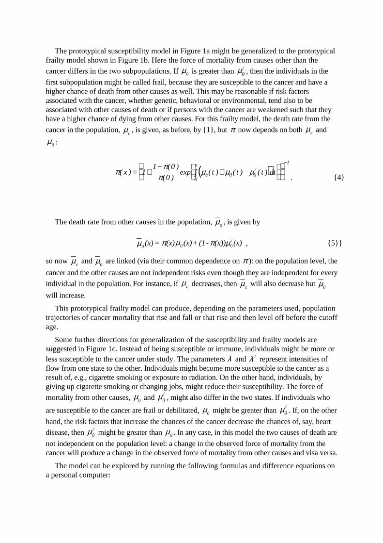
The prototypical susceptibility model in Figure 1a might be generalized to the prototypicalfrailty model shown in Figure 1b. Here the force of mortality from causes other than the

cancer differs in the two subpopulations. If 0µ is greater than 0

/µ , then the individuals in the

first subpopulation might be called frail, because they are susceptible to the cancer and have ahigher chance of death from other causes as well. This may be reasonable if risk factorsassociated with the cancer, whether genetic, behavioral or environmental, tend also to beassociated with other causes of death or if persons with the cancer are weakened such that theyhave a higher chance of dying from other causes. For this frailty model, the death rate from the

cancer in the population, c

µ , is given, as before, by {1}, but π now depends on both cµ and

0µ :

The death rate from other causes in the population, 0

µ , is given by

0 0(x) = (x) (x)+ (1- (x)) (x) ,µ π µ π µ0/ {5}}

so now c

µ and 0

µ are linked (via their common dependence on π ): on the population level, the

cancer and the other causes are not independent risks even though they are independent for every

individual in the population. For instance, if cµ decreases, then

cµ will also decrease but

0µ

will increase.

This prototypical frailty model can produce, depending on the parameters used, populationtrajectories of cancer mortality that rise and fall or that rise and then level off before the cutoffage.

Some further directions for generalization of the susceptibility and frailty models aresuggested in Figure 1c. Instead of being susceptible or immune, individuals might be more orless susceptible to the cancer under study. The parameters λ and /λ represent intensities offlow from one state to the other. Individuals might become more susceptible to the cancer as aresult of, e.g., cigarette smoking or exposure to radiation. On the other hand, individuals, bygiving up cigarette smoking or changing jobs, might reduce their susceptibility. The force of

mortality from other causes, 0µ and 0

/µ , might also differ in the two states. If individuals who

are susceptible to the cancer are frail or debilitated, 0µ might be greater than 0

/µ . If, on the other

hand, the risk factors that increase the chances of the cancer decrease the chances of, say, heart

disease, then 0/µ might be greater than 0

µ . In any case, in this model the two causes of death are

not independent on the population level: a change in the observed force of mortality from thecancer will produce a change in the observed force of mortality from other causes and visa versa.

The model can be explored by running the following formulas and difference equations ona personal computer:

( )ππ

πµ µ µ( )

( )

( )exp ( ) ( ) ( )/x t t t dtc

x

= +−

+ −∫

−

11 0

0 0 00

1

. {4}

As an illustration of this general point, consider the model shown in Figure 1d. In thismodel, individuals are assumed, at starting age zero, to be immune from some cancer: peoplegradually become susceptible to the cancer at a constant rate λ . Susceptible individuals areassumed not only to be susceptible to the cancer being studied, but also to a related set ofcancers. In terms of a multistage model, the transition from immune to susceptible can beconsidered a transition common to a group of cancers, a transition based on some environmentalor behavioral factor that is a risk factor for all the various cancers in the group. This simpletransition model was used to produce the curves shown in Figure 2b: the more important othercancers are as a cause of death, the more bowed is the trajectory for the cancer being studied.

In addition to demonstrating that there are a variety of ways in which selection in aheterogeneous population can cause the age trajectory of cancer rates to level off or evendecline, the various models presented above can be used to show that even substantialheterogeneity may produce only weak effects on age trajectories. Using the variantdiagrammed in Figure 1e, Peto [45] demonstrates that even in cases where predisposedindividuals – be they 1 percent, 10 percent or 50 percent of the total population – suffer 50times the incidence of some cancer compared with the rest of the population, the agetrajectory of cancer incidence in the population as a whole may closely mimic, at least up toage 75 or so, the age trajectory of a homogeneous population. Other variants of the modeldiagrammed in Figure 1c can produce similar results; some of the trajectories in Figures 2aand 2b are examples. Thus, although heterogeneity may be a possible explanation for some ofthe observed leveling off and decline in cancer trajectories, the absence of apparent levelingoff or decline does not imply homogeneity or even approximate homogeneity. This isreassuring because it is virtually certain that substantial heterogeneity exists, produced byvarious genetic, behavioral, and environmental risk factors, for cancers of all types. A keyquestion that thus arises and which will be addressed in subsequent sections is the possibleimpact heterogeneity might have on time trajectories and geographic variations, even in thosecases where the heterogeneity does not have a substantial effect on age trajectories.

More elaborate models, with many states of susceptibility or a continuous distribution ofsusceptibility and with susceptibility changing with age or time, can be developed [4, 31, 54,57, 60]. In empirical analyses of particular forms of cancer or other causes of death, it may beappropriate to use models complicated enough to capture the key details of the diseaseprocess. Here our purpose is not statistical inference but insight. We will henceforth illustrateour examples with a single model that captures the key feature driving the process; it turns outthat in all instances it is sufficient to use models as simple as the prototypical susceptibilitymodel in Figure 1a, for which the risk of the cancer is independent of other mortality risks, orthe prototypical frailty model in Figure 1b, for which the mortality risks are linked on thepopulation level although they are independent for all individuals.

2.3 Successive Apogees

p(0)= (0) , p (0)= 1- (0) ,/π π {6}

p(x+ )= p(x)+ [ (x)p (x) -( (x)+ (x)+ (x))p(x)] ,c∆ ∆ λ µ µ λ/ /0 {7}

/ /c

/ /p (x + ) = p (x)+ [ (x)p(x) - ( (x)+ (x)+ (x)) p (x)] ,∆ ∆ λ µ µ λ/ /0 {8}

π (x)= p(x) / (p(x)+ p (x)) ,/ {9}

c c c(x) = (x) (x)+ (1- (x)) (x) µ π µ π µ / . {10}

Figure 3a displays the age trajectories of incidence rates from cervical cancer for three birthcohorts of Icelandic women (redrawn from data in Hakama [18]). Similar patterns ofcrossover and successive apogees can be found for other cohorts, other countries, and otherforms of cancer, e.g., for cervical cancer in Denmark [18], cancer of the larynx for Frenchmales [53], cancer of the bone among Japanese males and females, and leukemia amongsurvivors of the atomic bomb attacks in Japan and lung cancer among insulation workmen[40].

The prototypical susceptibility model, shown in Figure 1a and described by formulas {1}and {3}, yields successive apogees that resemble observed patterns. One simulation ispresented in Figure 3b; in this simulation, the trajectories shift to the right as the mortality ratedeclines and the trajectories reach higher peaks as the proportion of the population susceptibleto the cancer increases. As indicated above, a variety of other heterogeneity models, includingmodels in which the observed rates of cervical cancer are increasing because competingcauses of death are decreasing, can be used to produce trajectories similar to those in Figures3a. We present Figure 3b, and the simple model underlying it, not as an explanation ofcervical cancer trends in Iceland but as an illustration of the fact that such trends are consistentwith the operation of selection in heterogeneous populations and hence might be partiallyaccounted for by an appropriate heterogeneity model.

Although clear examples of successive mortality apogees for successive cohorts areunusual, perhaps because the age trajectories are usually cutoff at some age like 75 or 80before the full effects of selection can be seen, examples of crossover or strong convergenceare more common, as illustrated by the various cohort graphs in Segi et al. [50] and Magnus[26]. An interesting instance of a crossover in incidence rates is given in Hanai et al. [19] forstomach cancer among males and females in Osaka, Japan, who were classified into histologicgroups. In addition, patterns of decline over time in age-specific rates at younger ages andincreases at older ages are evident for all cancers combined and for various specific cancers inJapan [50] and other countries: Figure 4, which displays the age trajectories of death ratesfrom cancer and from other causes among U.S. women in 1970 and 1980, shows a crossoverfor cancer at age 55.

Differential selection in a heterogeneous population, which has been widely accepted as atleast a partial explanation for mortality crossover and convergence in several areas [29, 56],may provide at least a partial explanation of these observations as well. In any case, underfairly general conditions [55], a decrease in mortality rates at younger ages will result, in aheterogeneous population, in an increase at older ages and a uniform decrease in the rates atall ages will result in an observed mortality trajectory that converges toward and may cross theprevious trajectory. It follows, however, from Peto’s [45] analysis, discussed above, that evenstrong heterogeneity and substantial cohort differences may not lead to noticeableconvergence. Consequently, absence of convergence cannot be taken as evidence that thepopulation is homogeneous.

2.4 The Falling Cancer Share

Death rates from cancer among U.S. women in 1980 rose more slowly with age than deathrates from other causes. As a result, cancer accounted for a declining share of deaths with age:the share of deaths accounted for by cancer fell from 43 percent at ages 50-54 to only 9percent at ages above 85. In contrast, cardiovascular diseases accounted for 28 percent ofdeaths at ages 50-54 and fully 71 percent at ages above 85. The declining cancer share andrising cardiovascular share, which can also be observed for males, other times, and othercountries [46], is an implication of the fact that cancer rates tend to rise even more slowly than

a power function, whereas cardiovascular disease death rates (and total death rates) riseexponentially. An interesting (and speculative) perspective on this can be developed by usinga simple model, like the one in Figure 1a, that recognizes that people differ in theirsusceptibility to cancer. It may be that among people who are susceptible to cancer, the forceof mortality from cancer is higher at all ages than the force of mortality from, say,cardiovascular disease. Indeed, the force of mortality from cancer among the susceptiblepopulation may be increasing exponentially. Nonetheless the observed age trajectory of cancermortality may cross over the cardiovascular disease trajectory.

In the prototypical susceptibility model, the population force of mortality from cancer isgiven by formulas {1} and {3}. Substituting {1} into {3} yields an integral equation for π (x) :

Given the trajectory of mc (x) and the value of π (0) , numerical methods can be applied tothis equation to estimate the trajectory of π (x) . Then, by using {1}, the trajectory of µc(x) canbe calculated. Thus, if the proportion of the population at age zero that is susceptible to cancer isspecified, it is possible to estimate the force of mortality from cancer among the susceptiblepopulation. In the model the force of mortality from cardiovascular diseases is the same for allindividuals, regardless of their susceptibility to cancer, so the individual and population deathrates from cardiovascular disease will be identical.

Figure 5 was constructed by taking the observed cardiovascular disease and cancermortality trajectories as given in the 1980 U.S. mortality statistics for females; it was assumedthat 25 percent of the synthetic cohort experiencing these rates were susceptible to cancer atthe starting age of 20. The observed age-specific death rate from cancer falls below the deathrate from cardiovascular disease after age 60. The model, however, indicates that the deathrate from cancer among susceptible individuals exceeds the death rate from cardiovasculardiseases at all ages on the graph. We emphasize that this result is presented as an illustrationonly; the model is simplistic and the data faulty: selection operates on real cohorts, notsynthetic ones. The point, however, remains: the age trajectory of cancer mortality forsusceptible individuals might rise considerable more quickly, reach considerably higherlevels, and have a different shape than the observed population trajectory.

3. Variation over Time and Place

3.1 Compensating Cancers

The incidence of different kinds of cancer varies enormously, sometimes by several orders ofmagnitude, among various countries and regions [14, 38]. For all forms of cancer combined,the variation tends to be less. Table 1 presents the age-adjusted death rates for various formsof cancer and for cancer at all sites for the country that ranked 1st and the country that ranked40th in a data set for 1978-9 compiled by the World Health Organization (and presented in[1]). (We chose rank 40 to avoid erroneous values associated with poor data collection andprocessing in some countries with very low reported rates; the data for the first rankedcountries appeared fairly reliable, given its consistency with values reported for countriesranked 2 and 3). With the exception of leukemia, the ratio of the rates for the various cancers

ππ

πµ π( )

( )

( )exp ( ) ( )x t t dtc

x

= +−

∫

−

11 0

0 0

1

. {11}

ranges from about 4 to about 9, in contrast with a ratio of 2 for all cancers combined.Apparently when some forms of cancer are unimportant, other forms grow in importance.

Table 1. Age-adjusted death rates per 100, 000 for various forms of cancer and for cancer atall sites for the 1st and 40th ranked country.

Cancer Sex For 1st

rankedcountry

For 40th

rankedcountry

Ratio

Oral M 20.3 2.2 9.2

F 7.2 0.8 9.0

Prostate M 41.0 5.4 7.6

Lung M 113.2 15.6 7.3

F 30.9 5.0 6.2

Colon & rectum M 34.0 5.7 6.0

F 29.5 7.7 3.9

Stomach M 66.1 14.4 4.6

F 33.5 7.2 4.6

Breast F 33.8 7.9 4.3

Uterus F 30.0 7.5 4.0

Leukemia M 9.6 3.9 2.5

F 6.3 2.8 2.3

All sites M 275.0 135.0 2.0

F 172.3 86.9 2.0

Source: [1].

A similar phenomenon can be observed over time: in various countries as some forms ofcancer have declined in importance, others have increased, so that total cancer rates tend to bemore steady than rates from particular forms of cancer. In the United States, for instance,age-adjusted lung cancer mortality rates have increased substantially over recent decades,rates for stomach cancer and cancer of the uterus have substantially declined, and variousother cancer rates have shown considerable fluctuation, but the overall cancer mortality ratehas remained relatively steady, showing only a small rate of increase [1, 39].

Such compensating changes are consistent with a model that assumes people differ in theirsusceptibility to cancer (or some set of cancers). A simple version of such a model is shown in

Figure 1f. The population death rates from the two forms of cancer, 1

c (x)µ and 2

c (x)µ , are

given by

µ π µci

ci(x)= (x) (x) , i = 1,2 {12}

where, following {3}, it can be shown that

Hence, the two trajectories for i

c (x)µ are linked. If 1

c (x)µ , say, declines, then π (x) will

grow and 2

c (x)µ will increase. Indeed, even if both 1

cµ and

2c

µ are declining, if more progress

is being made against cancer 1 than cancer 2, it may look, at ages old enough that selection hashad a major impact, as if cancer 2 is increasing. Table 2 summarizes the results of a simulationusing this model.

Table 2. Annual rates of progress in reducing death rates at various ages for cancer 1, cancer2, and cancer 1 and 2 combined, for the susceptible subpopulation and the entirepopulation

Annual rate of progress (in percent) in reducing death rate

from cancer 1 from cancer 2 from cancer 1 and 2

Age

Actual ratefor

susceptiblepopulation(in percent)

Observedrate forentire

population(in percent)

Actual ratefor

susceptiblepopulation(in percent)

Observedrate forentire

population(in percent)

Actual ratefor

susceptiblepopulation(in percent)

Observedrate forentire

population(in percent)

50 1 0.96 0.1 0.06 0.57 0.53

60 1 0.88 0.1 -0.02 0.57 0.44

70 1 0.68 0.1 -0.22 0.57 0.24

80 1 0.25 0.1 -0.65 0.57 -0.18

Source: Computer calculations using multiple susceptibility model, described in text with

π ( ) .0 0 05= and ci x b xµ ( ) = 1

5 , with bi chosen such that 0

75

c (x)dx = 0.5∫ µ1 and

0

75

c (x)dx = 0.333.∫ µ2

At all ages, progress is being made in reducing mortality from cancer 2 at a rate of 0.1percent per year. However, the observed rate of progress in reducing cancer 2 is much lessthan this and is negative at age 60 and subsequently. Note the magnitude of the observednegative rate of progress at ages 70 and 80 is 2.2 and 6.5 times the magnitude of the actualrate for susceptible individuals at these ages. The observed rate of progress in reducingmortality from cancer 1 is also less than the actual rate. This is another manifestation of theconvergence and crossover of mortality trajectories discussed above: saving susceptibleindividuals at younger ages reduces observed rates of progress in reducing mortality at olderages. For both forms of cancer combined, the overall rate of progress among susceptible

( )ππ

πµ µ( )

( )

( )exp ( ) ( )x t t dtc c

x

= +−

+∫

−

11 0

01 2

0

1

. {13}

individuals is 0.57 percent per year at all ages, but the observed overall rate of progress isconsiderably less at ages 60 and 70 and at age 80 it appears as it the overall cancer death rateis increasing.

3.2 Multiple Cancers

The hypothesis that some individuals may be more susceptible than other individuals toseveral different forms of cancer (or to cancer in general) seems to run counter to the widelyaccepted view that, as Cairns [6] puts it, "each of the major cancers behaves almost as anindependent entity; with few exceptions, people who have been successfully treated for onecancer are then neither more nor less likely in subsequent years to come down with a second,different variety." Schoenberg [48] reviews the evidence on multiple cancers and presents adetailed analysis of the Connecticut Tumor Registry. He concludes: "Results fornon-simultaneously diagnosed malignant tumors from Connecticut indicate that individualswith one malignant neoplasm have 1.29 times the risk of developing a new independentprimary tumor compared to individuals who never had cancer (P < 0.01). However, theincreased risk of multiple primary tumors is highly selective on a site-specific basis". Forexample, women with breast cancer had 1.9 times the risk of cancer of the corpus uteri and0.5 times the risk of cancer of the pancreas; men with lung cancer had 6.5 times the risk ofcancer of the kidney and men with cancer of the colon had 0.5 times the risk of lung cancer.

To understand the relationship of statistics such as these to the heterogeneity modelsdiscussed in this paper, consider the model shown in Figure 1g. There are two kinds of cancerin the model and two kinds of individuals. One cohort of individuals is more susceptible toboth kinds of cancer than the other cohort. For simplicity it is assumed that the two cancershave identical, independent incidence rates for each of the two groups. Death is ignored in themodel because the concern is with multiple cancers among those who survive to somespecified age.

Let r denote the relative risk of incidence of either cancer for the more susceptiblecompared with the less susceptible group; we will call r the relative risk of cancer incidence.Let R denote the relative risk of cancer 2 among those who have developed cancer 1 comparedwith those who have not developed cancer 1; we will call R, which is essentially equivalent tothe statistic used by Schoenberg, the relative risk of cancer 2 prevalence. The question is: whatis the relationship of R to r? The answer, surprisingly, is that the value of R tells us very littleabout the value of r; and that R can be fairly low (e.g., 1.29) when r is extremely large or eveninfinite.

Let 0 1 2n (x), n (x), n (x) , and 12n (x) denote the number of individuals in the less susceptiblecohort at age x who have no cancer, the first or the second cancer, or both, respectively, and usethe same notation with a prime to denote the numbers for the more susceptible cohort. It is notdifficult to show that for both groups:

and

i 0 0 0n (x)= n (0)n (x) - n (x) , i = 1,2 {14}

12 0 0 0 0n (x)= n (0)+ n (x)- 2 n (0)n (x) . {15}

The value of 0n (x) depends on the function chosen for the transition rate λ . If λ is assumedto be a power function

then

and

The value of R(x), which is the ratio of the probability of cancer 2 given cancer 1 to theprobability of cancer 2 given the absence of cancer 1, can then be calculated by:

Table 3 presents the value of R for various values of the relative risk of cancer incidence, r,suffered by persons in the more susceptible group.

λ = bx ,k {16}

n x nb

kx k

0 010

2

1( ) ( )exp= −

+

+ {17}

n x nrb

kxk

0 010

2

1/ /( ) ( ) exp= −

+

+ . {18}

R(x)=

n (x)+n (x)

n (x)+ n (x)+ n (x)+ n (x)

n (x)+ n (x)

n (x)+ n (x)+ n (x)+ n (x)

.

12 12

1/

1 12 12

2/

2

0/

0 2/

2

/

/

{19}

Table 3. The values of R, the relative risk of cancer 2 prevalence, at age 65, for various valuesof r, the relative risk of cancer incidence, and, 0π the proportion who are highlysusceptible.

0π r R

0.5 ∞ 2.04

0.5 100.0 2.00

0.5 10.0 1.69

0.5 3.0 1.25

0.5 1.0 1.00

0.1 ∞ 10.35

0.9 ∞ 1.12

0.5 3.3 1.29

0.75 16.0 1.29

0.78 100.0 1.29

0.78 ∞ 1.29

Source: Calculations based on model described in text with k = 6 and b chosen such that

0

756bx dx = 0.1∫ for the more susceptible group. Using a value of k of 2 or 8 or a value of b a

hundred times lower or twice as high hardly alters the results.

As the table suggests, the value of R is essentially independent of the value of r when r is100 or more. When such a large differential exists between the more and less susceptiblegroups, R is approximately equal to the inverse of the proportion of the population at age zerothat is susceptible. Thus a value of R of about 2 is consistent with a model in which about halfthe population is highly susceptible to both cancers. Even when r is considerably less than100, the value of r tends to be much larger than the value of R. For instance, a value of R of1.25 is consistent with a model in which half the population is three times more susceptible toboth kinds of cancer than the other half of the population; if R is 2, then the more susceptiblegroup could be a third of the total population with a relative risk of 10 or half of the totalpopulation with a relative risk of 100 or more.

A simple example helps provide an explanation of the difference between the relative riskof cancer incidence, r, and the relative risk of cancer 2 prevalence, R. Suppose half thepopulation is highly susceptible to cancer 1 and 2 and the other half is essentially immune.More specifically, assume that the more susceptible group faces a risk of 2 percent ofdeveloping either cancer by age 65 whereas the risk for the less susceptible group is athousand times less. If someone gets cancer 1 before age 65, that person is almost certainly amember of the highly-susceptible group and thus has a two percent chance of developingcancer 2 by age 65. Because the chance of either cancer is low, the fact that someone does nothave cancer 1 tells us very little about which group the person is in. Hence, since people

without cancer 1 have about a fifty percent chance of being susceptible, their chance of havingcancer 2 by age 65 is half of 2 percent. Thus, having cancer 1 only doubles the chance ofcancer 2, even though having cancer 1 is very strong evidence that a person is highlysusceptible and highly susceptible people face 1000 times the risk of cancer 1 or 2.

For some pairs of cancers, people having one cancer seem to be less likely to have thesecond cancer than people without the first cancer [48]. This could imply that people highlysusceptible to the first cancer have low susceptibility to the second cancer. Alternatively,however, it may be that people in one group are more susceptible to both kinds of cancer,given that they have neither cancer but that getting the first cancer lowers the chances ofgetting the second cancer, because the effects of treatment, of physiological or behavioralchanges, or whatever.

As an example, consider again the model in Figure 1g, but now suppose that the fourincidence rates, the λ ’s, on the bottom half of the diagram are less than the four λ ’s on the tophalf. Specifically, assume that the incidence of either of the cancers among people with the othercancer is some fraction of the incidence among people without the other cancer. Table 4 presentssome values of the relative risk of cancer 2 prevalence, R, corresponding to various values of thisfraction and various values of the relative risk of cancer incidence, r.

Table 4. The value of R, the relative risk of cancer 2 prevalence at age 65, for various valuesof r, the relative risk of cancer incidence ′λ λ/ , the relative risk of incidence ofsecond cancer, and 0π , the proportion who are highly susceptible.

0π ′λ λ/ r R

0.50 0.4 ∞ 0.82

0.50 0.2 ∞ 0.41

0.50 0.5 10 0.86

0.25 0.5 3 0.78

0.75 0.6 ∞ 0.81

Source: Computer calculations using numerical methods to approximate the model

described in the text, with k = 6 and b chosen such that 0

756bx dx = 0.1∫ for the more

susceptible group.

The parameters used result in values of the relative risk of cancer 2 prevalence that are lessthan one. These values, which might be interpreted as indicating that people who are moresusceptible to the first cancer are less susceptible to the second, were produced, however, by amodel in which part of the population is more susceptible to both cancers.

The model of multiple cancer presented in Figure 1g is highly simplified. Furthermore, theevidence concerning multiple cancer must, as Schoenberg [48] discusses, be used with greatcaution. Nonetheless, the model and the evidence are perhaps sufficient to draw the

conclusion that the current evidence about multiple cancer is not inconsistent with theexistence of substantial differences among individuals in their susceptibility to groups ofcancers and perhaps even to cancer in general.

3.3 Why is Cancer Mortality Increasing over Time?

As shown in Figure 6, the mortality rate from cancer among U.S. females aged 60-64 hasremained fairly stable since 1900, whereas total mortality has fallen to close to a third of its1900 level and cardiovascular mortality rates have been cut more than 50 percent since 1950.Roughly similar patterns hold at other ages and for age-standardized rates, for males as well asfemales, although for males there is more of an increase in cancer rates, largely due to lungcancer. Much attention has been devoted to trying to determine trends in rates of cancerincidence and mortality, the causes of such trends, and the implications for policy [14, 26]. Asexplained in this section, heterogeneity makes such efforts even more difficult than previouslyrecognized.

Before discussing why, it is useful to consider two other pieces of evidence. Figure 4displays the age-specific U.S. female mortality trajectories for cancer and for all causes ofdeath other than cancer for 1970 and for 1980. It is apparent that rapid progress has been madeagainst causes of death other than cancer. For cancer, on the other hand, there is evidence ofprogress at younger ages and evidence of higher death rates at older ages.

If, instead of following a single country over time, a variety of countries are compared atsome point in time, a pattern emerges that may be similar in origin to the increasing relativeimportance of cancer over time: the countries with the highest death rates from other causestend to have the lowest death rates from cancer. For instance, using age-adjusted death ratesfor 1975 for 50 countries with widely varying rates ([50], Appendix Table I), the Spearmancorrelation coefficient between the rate for malignant neoplasms and the rate for all othercauses of death is -0.27 for males and -0.39 for females. As in the case of temporal trends, itlooks from this kind of cross-sectional data as if progress against other causes of death isassociated with an increase in cancer mortality rates.

Hence, it may prove to be significant that observed cancer mortality rates for a populationmay decrease slowly, stay roughly level, or even increase even though the risks of cancer forthe individuals that comprise the population are decreasing. There are three main mechanismsin heterogeneous populations that can produce such results.

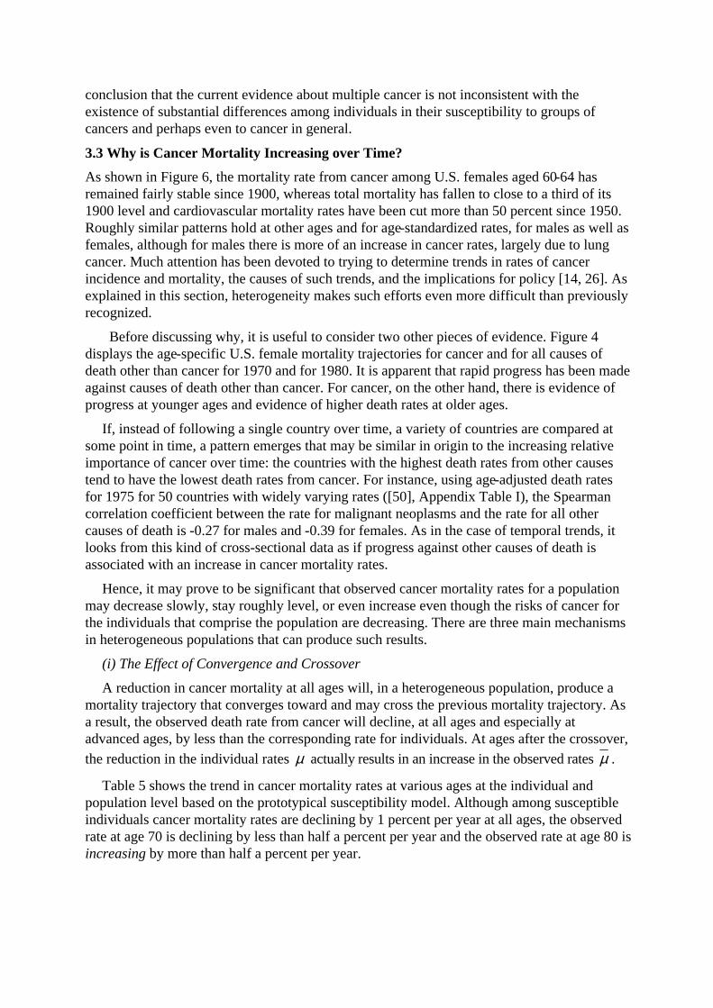
(i) The Effect of Convergence and Crossover

A reduction in cancer mortality at all ages will, in a heterogeneous population, produce amortality trajectory that converges toward and may cross the previous mortality trajectory. Asa result, the observed death rate from cancer will decline, at all ages and especially atadvanced ages, by less than the corresponding rate for individuals. At ages after the crossover,

the reduction in the individual rates µ actually results in an increase in the observed rates µ .

Table 5 shows the trend in cancer mortality rates at various ages at the individual andpopulation level based on the prototypical susceptibility model. Although among susceptibleindividuals cancer mortality rates are declining by 1 percent per year at all ages, the observedrate at age 70 is declining by less than half a percent per year and the observed rate at age 80 isincreasing by more than half a percent per year.

Table 5. Annual rate of progress in reducing cancer death rates at various ages, for thesusceptible subpopulation and the entire population.

Annual rate of progress (in percent) in reducing cancer death rate:

Age

Actual rate forsusceptiblesubpopulation(in percent)

Observed rate forentire population

(in percent)

50 1 0.9660 1 0.8370 1 0.4480 1 -0.61

Source: Computer calculations using prototypical susceptibility model, described in text,

with π ( ) .0 0 25= and c x bxµ ( ) = 6 , with b chosen such that 0

75

c(x)= 0.8∫ µ .

(ii) The Effect of Compensating Cancers

Progress against one form of cancer may be offset by an observed rise in other forms forwhich susceptible individuals face higher risks. As illustrated above in Table 2, even ifprogress is being made against all forms of cancer, if the rates of progress differ for differentforms of cancer, it may appear as if certain cancers are growing in importance. The observeddeath rate, at any age and especially at older ages, from all forms of cancer will, as a result,decline more slowly than the actual death rate among susceptible individuals.

(iii) The Effect of Progress Against Other Causes

A similar effect will result if individuals who are susceptible to cancer are also moresusceptible to other forms of death, as in the prototypical frailty model. In this model, theobserved age-specific death rates from cancer and other causes are linked as described byformulas {4} and {5}. The formulas imply that a proportional decrease in the death rates fromother causes among the frailer and more robust subcohorts may result in an increase in theobserved death rates from cancer, even though the death rates from cancer among susceptibleindividuals remain the same. Indeed, even if the death rates from cancer among susceptibleindividuals decrease somewhat, the observed death rates from cancer may increase.

The statistics in Table 6 provide an illustration.

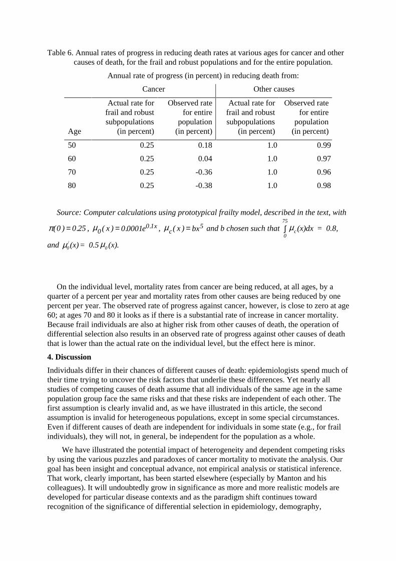
Table 6. Annual rates of progress in reducing death rates at various ages for cancer and othercauses of death, for the frail and robust populations and for the entire population.

Annual rate of progress (in percent) in reducing death from:

Cancer Other causes

Age

Actual rate forfrail and robustsubpopulations

(in percent)

Observed ratefor entire

population(in percent)

Actual rate forfrail and robustsubpopulations

(in percent)

Observed ratefor entire

population(in percent)

50 0.25 0.18 1.0 0.99

60 0.25 0.04 1.0 0.97

70 0.25 -0.36 1.0 0.96

80 0.25 -0.38 1.0 0.98

Source: Computer calculations using prototypical frailty model, described in the text, with

π ( ) .0 0 25= , 00 10 0001µ ( ) . .x e x= , c x bxµ ( ) = 5 and b chosen such that

0

75

c(x)dx = 0.8,∫ µ

and µ µ0 0(x)= 0.5 (x)./

On the individual level, mortality rates from cancer are being reduced, at all ages, by aquarter of a percent per year and mortality rates from other causes are being reduced by onepercent per year. The observed rate of progress against cancer, however, is close to zero at age60; at ages 70 and 80 it looks as if there is a substantial rate of increase in cancer mortality.Because frail individuals are also at higher risk from other causes of death, the operation ofdifferential selection also results in an observed rate of progress against other causes of deaththat is lower than the actual rate on the individual level, but the effect here is minor.

4. Discussion

Individuals differ in their chances of different causes of death: epidemiologists spend much oftheir time trying to uncover the risk factors that underlie these differences. Yet nearly allstudies of competing causes of death assume that all individuals of the same age in the samepopulation group face the same risks and that these risks are independent of each other. Thefirst assumption is clearly invalid and, as we have illustrated in this article, the secondassumption is invalid for heterogeneous populations, except in some special circumstances.Even if different causes of death are independent for individuals in some state (e.g., for frailindividuals), they will not, in general, be independent for the population as a whole.

We have illustrated the potential impact of heterogeneity and dependent competing risksby using the various puzzles and paradoxes of cancer mortality to motivate the analysis. Ourgoal has been insight and conceptual advance, not empirical analysis or statistical inference.That work, clearly important, has been started elsewhere (especially by Manton and hiscolleagues). It will undoubtedly grow in significance as more and more realistic models aredeveloped for particular disease contexts and as the paradigm shift continues towardrecognition of the significance of differential selection in epidemiology, demography,

actuarial mathematics, reliability engineering, and other population disciplines. Examples ofthe application of heterogeneity modeling to phenomena as diverse as fertility, divorce, theextinction of families of species, equipment failure, dental caries, accident proneness and thediscovery of new petroleum deposits are reviewed in Vaupel and Yashin [55, 56].

This paper began with a list of seven puzzles and paradoxes of cancer epidemiology. Itsfindings can be summarized using the same list. The effects of differential selection in apopulation in which individuals vary in their susceptibility to cancer in general, or to variousforms of cancer, or to various causes of death may partially account for:

• the leveling off and decline of cancer incidence and mortality rates with age,

• the fact that a greater proportion of deaths are from cancer around ages 50 or 60 than atolder ages,

• the greater variation among countries in incidence and mortality rates from various formsof cancer than in incidence and mortality rates from cancer in general,

• the convergence and crossover of the age trajectories of cancer rates for two cohorts,from different time periods, countries, histological types, etc.,

• the negative correlation among countries in the mortality rates from cancer vs. othercauses of death,

• the increase over time in mortality for some forms of cancer and decrease for otherforms, and

• the tendency for cancer incidence and mortality rates to somewhat increase, whereasmortality rates from almost all other major causes of death, including heart disease andcerebrovascular disease, are declining.

In addition, two other findings are worth highlighting.

First, a variety of different heterogeneity models can produce qualitatively similar mortalitypatterns and trajectories. Simple susceptibility and frailty models that only distinguish twokinds of individuals were sufficient to illustrate the points made in this paper. It seems likely,though, that more elaborate models will fit empirical data better than such simple models.Even if some heterogeneity models, e.g. the prototypical susceptibility model, can be ruled outbecause of evidence, say, that few if any individuals are completely immune to cancer, other,more elaborate models may still be plausible. Indeed, individuals differ from each other alongso many important risk factors that it seems incontrovertible that populations areheterogeneous: the question is when does this heterogeneity have an important effect onepidemiological statistics and, when it does, how should the heterogeneity be modeled?

Second, even substantial differences among individuals in their susceptibility to cancer orto some form of cancer may not produce a noticeable impact on the observed age trajectory ofcancer mortality in a population. The impact of such differences, however, may significantlyalter patterns of cancer mortality over time or place. Therefore, the absence of strongheterogeneity effects in some set of cancer statistics should not be assumed to exclude strongeffects in other sets of cancer statistics.

These various findings open up new hypotheses and new research directions. Even less isknown about cancer epidemiology than was previously thought, but more can be learned bysystematically considering the effects of differential selection in heterogeneous populations.Some key facts that were assumed self-evident – such as the belief that little or no progress is

being made in reducing rates of overall cancer mortality – may still be correct, but thatremains to be established.

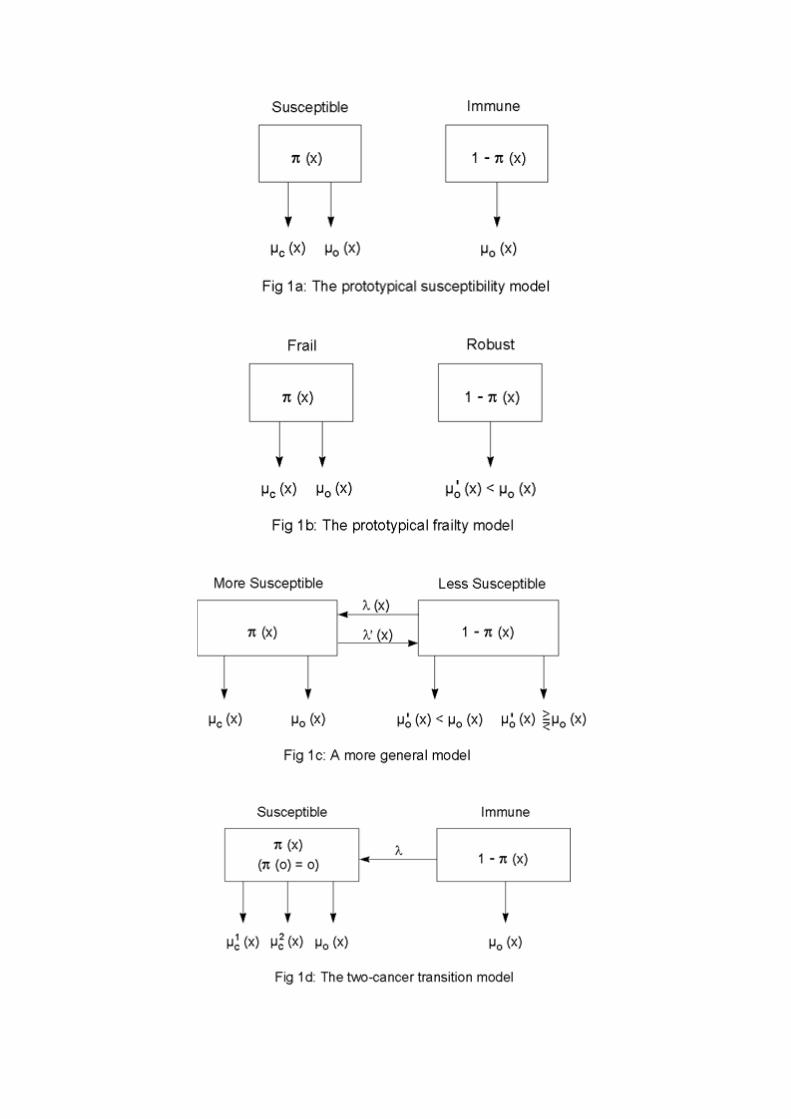
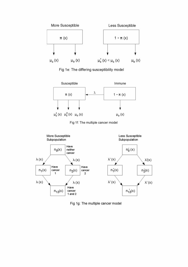
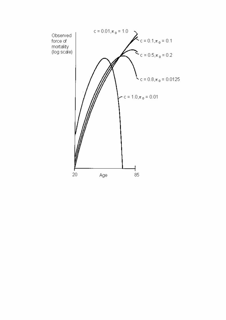
Figure 2a.

The observed force of mortality from cancer from age 20 to 85 produced by theprototypical susceptibility model for 5 pairs of parameter values. See text for details.

Figure 2b.

The observed force of mortality from cancer 1 from age 20 to 85 produced by two-cancer transition model for three levels of mortality from cancer 2. See text for details

of the model. The following parameters were used: ( )λ µ= =0 01 15. , c x bx with b chosen

such that ( ) ( )µ µc cx dx x bx10

75

250 01∫ = =. ; with b chosen such that ( )µcx

x

x dx0∫ = 0, 0.5 and

0.9, respectively, for the three curves, and ( )µ010 0001x e x= . . .

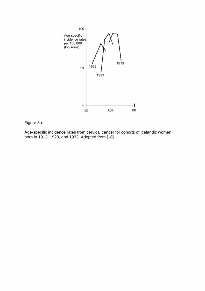
Figure 3a.

Age-specific incidence rates from cervical cancer for cohorts of Icelandic womenborn in 1913, 1923, and 1933. Adopted from [18].

Figure 3b.

Age-specific incidence rates from age 20 to 85 produced by the prototypicalsusceptibility model for three sets of parameter values. See text for details of model.For the three curves from left to right π0 is 0.012, 0.02, and 0.022 and µ(x) = ax6,

where a is chosen such that 0

t

∫ µ(x)dx = 1, 0.99, and 0.9 for t = 65, 70, and 75,

respectively.

Figure 4.

Death rates in 1980 relative to 1970 from cancer and other causes for U.S. womenfrom age 20 to 85.

Figure 5.

Annual death rates from cancer and cardiovascular diseases in 1980 for U.S. womenfrom age 20 to 85. The death rates from cancer among susceptibles were calculatedas described in the text, with π0, the proportion susceptible at the starting age (of 20)equal to 0.25.

Figure 6.

Annual death rates from all causes, cardiovascular disease, and cancer from 1900 to1980 for U.S. women aged 60 - 65.

References

1. American Cancer Society. Cancer Facts and Figures. New York: American CancerSociety; 1985.

2. Armitage P, Doll R. Age Distribution of Cancer. British Journal of Cancer 1954;8:1-12.

3. Armitage, P, Doll R. Stochastic models for carcinogenesis. Proceedings of the FourthBerkeley Symposium on Mathematical Statistics and Probability. Biology and problems ofhealth, vol IV. Berkeley: University of California Press; 1961. p. 19.

4. Beard RJ. A theory of mortality based on actuarial, biological, and medical considerations.Proceedings of the International Population Conference. London: International Union forthe Scientific Study of Population; 1963. p. 257.

5. Burch PRJ. Natural and radiation carcinogenesis in man: 1. theory of initiation phase.Proceedings of the Royal Society B 1965;162:223-39.

6. Cairns J. Cancer: Science and society. San Francisco: Freeman; 1978.

7. Cairns J, Lyon JL, Skolnick M, editors. Cancer incidence in defined populations. BanburyReport; 4. Cold Spring Harbor, NY: Cold Spring Harbor Laboratory; 1980.

8. Chiang CL. Introduction to stochastic processes in biostatistics. New York: Wiley; 1968.

9. Cohen J, Liu L. Competing Risks Without Independence. Manuscript. 1984.

10. Cook PJ, Doll R, Fellingham SA. A mathematical model for the age distribution of cancerin man. International Journal of Cancer 1969;4(1):93-112.

11. Day NE, Charnay B. Time trends, cohort effects, and aging as influence on cancerincidence. In: Magnus K, editor. Trends in cancer incidence: causes and practicalimplications. Proceedings of a symposium; 1980 Aug 6-7; Oslo, Norway. Washington:Hemisphere Publishing; 1982. p. 51.

12. DeVita VT Jr, Hellman S, Rosenberg SA, editors. Cancer: principles and practice ofoncology. 2nd ed. Philadelphia: Lippincott; 1985.

13. Doll R. The epidemiology of cancer. Cancer 1980;45(10):2475-85.

14. Doll R, Peto R. The causes of cancer: quantitative estimates of avoidable risks of cancer inthe United States today. Journal of the National Cancer Institute 1981;66(6):1191-308.

15. Economos AC. Rate of aging, rate of dying and the mechanism of mortality. Archives ofGerontology & Geriatrics 1982;1(1):3-27.

16. Engel A, Larsson T, editors. Cancer and aging. Proceedings of the Thule InternationalSymposium on Cancer and Aging; 1967 Sep 26-28; Stockholm, Sweden. Stockholm:Nodriska Bokhandeln; 1968.

17. Fraumeni JF Jr, editor. Persons at high risk of cancer: an approach to cancer etiology andcontrol. Proceedings of a conference; 1974 Dec 10-12; Key Biscayne, Florida. New York:Academic Press; 1975.

18. Hakama M. Trends in the incidence of cervical cancer in the Nordic countries. In: MagnusK, editor. Trends in cancer incidence: causes and practical implications. Proceedings of asymposium; 1980 Aug 6-7; Oslo, Norway. Washington: Hemisphere Publishing; 1982. p.279.

19. Hanai A, Fujimoto I, Taniguchi H. Trends of stomach cancer incidence and histologicaltypes in Osaka. In: Magnus K, editor. Trends in cancer incidence: causes and practicalimplications. Proceedings of a symposium; 1980 Aug 6-7; Oslo, Norway. Washington:Hemisphere Publishing; 1982. p. 143.

20. Hanszel W. Migrant studies. In: Schottenfeld D, Fraumeni JF Jr, editors. Cancerepidemiology and prevention. Philadelphia: Saunders; 1982. p. 194-207.

21. Heston JF et al [Cusano MM, Young JL Jr, editors]. Forty-five years of cancer incidencein Connecticut: 1935-79. National Cancer Institute Monograph; 70. Washington, DC: forsale only by the Supt. of Docs., U.S. G.P.O.; 1986. p. 1.

22. Hiatt HH, Watson JD, Winsten JA, editors. Origins of human cancer. Book C: Human riskassessment. Cold Spring Harbor conferences on cell proliferation; 4. Proceedings of aconference; 1976 Sep. Cold Spring Harbor, NY: Cold Spring Harbor Laboratory; 1977.

23. Knudson AG Jr. Genetic predisposition to cancer. In: Hiatt HH, Watson JD, Winsten JA,editors. Origins of human cancer. Book C: Human risk assessment. Cold Spring Harborconferences on cell proliferation; 4. Proceedings of a conference; 1976 Sep. Cold SpringHarbor, NY: Cold Spring Harbor Laboratory; 1977. p. 45.

24. Keyfitz N. Applied mathematical demography. 2nd ed. New York: Springer; 1985.

25. Kvaale G. Incidence trends in the nordic countries. In: Magnus K, editor. Trends in cancerincidence: causes and practical implications. Proceedings of a symposium; 1980 Aug 6-7;Oslo, Norway. Washington: Hemisphere Publishing; 1982. p. 185.

26. Magnus K, editor. Trends in cancer incidence: causes and practical implications.Proceedings of a symposium; 1980 Aug 6-7; Oslo, Norway. Washington: HemispherePublishing; 1982.

27. Manton KG, Stallard E. A two-disease model of female breast cancer: mortality in 1969among white females in the United States. Journal of the National Cancer Institute1980;64(1):9-16.

28. Manton KG, Stallard E. A population-based model of respiratory cancer incidence,progression, diagnosis, treatment, and mortality. Computers & Biomedical Research1982;15(4):342-60.

29. Manton KG, Stallard E. Methods for evaluating the heterogeneity of aging processes inhuman populations using vital statistics data: explaining the black/white mortalitycrossover by a model of mortality selection. Human Biology 1981;53(1):47-67.

30. Manton KG, Stallard E. Bioactuarial models of national mortality time series data. HealthCare Financing Review 1982;3(3):89-109.

31. Manton KG, Stallard E. Recent trends in mortality analysis. Orlando, FL: Academic Press;1984.

32. Manton KG, Stallard E, Burdick D, Tolley HD. A stochastic compartment model ofstomach cancer with correlated waiting time distributions. International Journal ofEpidemiology 1979;8(3):283-91.

33. Manton KG, Stallard E, Vaupel JW. Alternative models for the heterogeneity of mortalityrisks among the aged. Journal of the American Statistical Association 1986;81(395):635-44.

34. Miller DG. On the nature of susceptibility to cancer. Cancer 1980;46:1307-18.

35. Moolgavkar SH. Carcinogenesis modeling: from molecular biology to epidemiology.Annual Review of Public Health 1986;7:151-69.

36. Mueller H, Weber W, editors. Familial cancer. Proceedings of the 1st InternationalResearch Conference on Familial Cancer; 1985 Sep 16-21; Basel, Schweiz. Basel: Karger;1985.

37. Muir CS. Epidemiological identification of cancer hazards. In: Nieburgs HE, editor.Prevention and detection of cancer. Part 2; Detection; vol 1: high risk markers, detectionmethods and management. Proceedings of the Third International Symposium onDetection and Prevention of Cancer; 1976 Apr 26 to May 1; New York. New York:Dekker; 1978. p. 53.

38. Muir CS, Nectoux J. International patterns of cancer. In: Schottenfeld D, Fraumeni JF Jr,editors. Cancer epidemiology and prevention. Philadelphia: Saunders; 1982. p. 119-37.

39. Newell GR. Epidemiology of Cancer. In: DeVita VT Jr, Hellman S, Rosenberg SA,editors. Cancer: principles and practice of oncology. 2nd ed. Philadelphia: Lippincott;1985. p. 151.

40. Nicholson WJ. Selection factors in cohort studies. National Cancer Institute Monograph1985;67:111-5.

41. Nieburgs HE, editor. Prevention and detection of cancer. Part 2; Detection; vol 1: high riskmarkers, detection methodes and management. Proceedings of the Third InternationalSymposium on Detection and Prevention of Cancer; 1976 Apr 26 to May 1; New York.New York: Dekker; 1978.

42. Nordling CO. A new theory on the cancer-inducing mechanism. British Journal of Cancer1953;7:68-72.

43. Ooi WL, Elston RC, Chen VW, Bailey-Wilson JE, Rothschild H. Increased familial riskfor lung cancer. Journal of the National Cancer Institute 1986;76(2):217-222.

44. Peto R. Epidemiology, multistage models, and short-term mutagenicity tests. In: Hiatt HH,Watson JD, Winsten JA, editors. Origins of human cancer. Book C: Human riskassessment. Proceedings of a conference; 1976 Sep. Cold Spring Harbor, NY: Cold SpringHarbor Laboratory; 1977. p. 1403.

45. Peto J. Genetic predisposition to cancer. In: Cairns J, Lyon JL, Skolnick M, editors.Cancer incidence in defined populations. Banbury Report; 4. Cold Spring Harbor, NY:Cold Spring Harbor Laboratory; 1980. p. 203.

46. Preston SH, Keyfitz N, Schoen R. Causes of death: life tables for national populations.New York: Seminar Press; 1972.

47. Sandstad B. Prediction of cancer incidence based on cohort analysis. In: Magnus K, editor.Trends in cancer incidence: causes and practical implications. Proceedings of asymposium; 1980 Aug 6-7; Oslo, Norway. Washington: Hemisphere Publishing; 1982.

48. Schoenberg BS. Multiple primary malignant neoplasms: the Connecticut experience,1935-1964. Recent results in cancer research; 58. Berlin; New York: Springer; 1977.

49. Schottenfeld D, Fraumeni JF Jr, editors. Cancer epidemiology and prevention.Philadelphia: Saunders; 1982.

50. Segi M, Tominaga S, Aoki K, Fujimoto I, editors. Cancer mortality and morbiditystatistics: Japan and the world. GANN monograph on cancer research; 26. Tokyo: JapanScientific Societies Press; 1981.

51. Stern AC, editor. The effect of air pollution. Air pollution; 2: Environmental Sciences.New York: Academic Press; 1977.

52. Teppo L. Incidence trends of melanoma of the skin in Finland by histological type. In:Magnus K, editor. Trends in cancer incidence: causes and practical implications.Proceedings of a symposium; 1980 Aug 6-7; Oslo, Norway. Washington: HemispherePublishing; 1982. p. 393.

53. Tuyns AJ. Incidence trends of laryngeal cancer in relation to national alcohol and tobaccoconsumption. In: Magnus K, editor. Trends in cancer incidence: causes and practicalimplications. Proceedings of a symposium; 1980 Aug 6-7; Oslo, Norway. Washington:Hemisphere Publishing; 1982. p. 199.

54. Vaupel JW, Manton KG, Stallard E. The impact of heterogeneity in individual frailty onthe dynamics of mortality. Demography 1979;16(3):439-54.

55. Vaupel JW, Yashin AI. The deviant dynamics of death in heterogeneous populations.Sociological Methodology 1985;15:179-211.

56. Vaupel JW, Yashin AI. Heterogeneity’s ruses: some surprising effects of selection onpopulation dynamics. American Statistician 1985;39(3):176-85.

57. Vaupel JW, Yashin AI, Manton KG. Debilitation’s aftermath: stochastic process models ofmortality. Mathematical Population Studies 1986;1(1):21-48.

58. Waterhouse J et al, editors. Cancer incidence in five continents: a technical report. Vol 3.IARC scientific publications, 0300-5085; 42. Lyon: International Agency for Research onCancer; 1976.

59. Watson G. Age incidence curves for cancer. Proceedings of the National Academy ofScience 1977;74(4):1341-2.

60. Yashin AI, Manton KG, Vaupel JW. Mortality and aging in a heterogeneous population: astochastic process model with observed and unobserved variables. Theoretical PopulationBiology 1985;27(2):157-75.

61. Yashin AI, Manton KG, Stallard E. Dependent competing risks: a stochastic processmodel. Journal of Mathematical Biology 1986;24(2):119-140.