capital markets and portfolio theory, roland portait
TRANSCRIPT
8/3/2019 Capital Markets and Portfolio Theory, Roland Portait
http://slidepdf.com/reader/full/capital-markets-and-portfolio-theory-roland-portait 1/102
Capital Markets and PortfolioTheory
Roland PortaitFrom the class notes taken by Peng Cheng
Novembre 2000

8/3/2019 Capital Markets and Portfolio Theory, Roland Portait
http://slidepdf.com/reader/full/capital-markets-and-portfolio-theory-roland-portait 2/102
2
8/3/2019 Capital Markets and Portfolio Theory, Roland Portait
http://slidepdf.com/reader/full/capital-markets-and-portfolio-theory-roland-portait 3/102
Table of Contents
Table of Contents
PART I Standard (One Period) Portfolio Theory . . . . . . . . . . . . . . . . . . . . . 1
1 Portfolio Choices . . . . . . . . . . . . . . . . . . . . . . . . . . . . . . . . . . . . . . . . . . . . . . . . . . . . . . . . 21.A Framework and notations. . . . . . . . . . . . . . . . . . . . . . . . . . . . . . . . . . . . . . . . . . . . . 2
1.A.i No Risk-free Asset . . . . . . . . . . . . . . . . . . . . . . . . . . . . . . . . . . . . . . . . . . . . . . . . 21.A.ii With Risk-free Asset . . . . . . . . . . . . . . . . . . . . . . . . . . . . . . . . . . . . . . . . . . . . . . 4
1.B Efficient portfolio in absence of a risk-free asset . . . . . . . . . . . . . . . . . . . . . . 61.B.i Effi ciency criteria . . . . . . . . . . . . . . . . . . . . . . . . . . . . . . . . . . . . . . . . . . . . . . . . . 61.B.ii Effi cient portfolio and risk averse investors . . . . . . . . . . . . . . . . . . . . . . . . . . . 81.B.iii Effi cient set . . . . . . . . . . . . . . . . . . . . . . . . . . . . . . . . . . . . . . . . . . . . . . . . . . . . . . 91.B.iv Two funds separation (Black) . . . . . . . . . . . . . . . . . . . . . . . . . . . . . . . . . . . . . 1 0
1.C Efficient portfolio with a risk-free asset . . . . . . . . . . . . . . . . . . . . . . . . . . . . . . 111.D HARA preferences and Cass-Stiglitz 2 fund separation . . . . . . . . . . . . . . 14
1.D.i HARA (Hyperbolic Absolute Risk Aversion) . . . . . . . . . . . . . . . . . . . . . . . . 141.D.ii Cass and Stiglitz separation . . . . . . . . . . . . . . . . . . . . . . . . . . . . . . . . . . . . . . . 1 5
2 Capital Market Equilibrium . . . . . . . . . . . . . . . . . . . . . . . . . . . . . . . . . . . . . . . . . . 172.A CAPM . . . . . . . . . . . . . . . . . . . . . . . . . . . . . . . . . . . . . . . . . . . . . . . . . . . . . . . . . . . . . . . 17
2.A.i The Model . . . . . . . . . . . . . . . . . . . . . . . . . . . . . . . . . . . . . . . . . . . . . . . . . . . . . 1 7
2.A.ii Geometry . . . . . . . . . . . . . . . . . . . . . . . . . . . . . . . . . . . . . . . . . . . . . . . . . . . . . . 1 92.A.iii CAPM as a Pricing and Equilibrium Model . . . . . . . . . . . . . . . . . . . . . . . . . 192.A.iv Testing the CAPM . . . . . . . . . . . . . . . . . . . . . . . . . . . . . . . . . . . . . . . . . . . . . . 2 1
2.B Factor Models and APT. . . . . . . . . . . . . . . . . . . . . . . . . . . . . . . . . . . . . . . . . . . . . 212.B.i K -factor models . . . . . . . . . . . . . . . . . . . . . . . . . . . . . . . . . . . . . . . . . . . . . . . . . 2 12.B.ii APT . . . . . . . . . . . . . . . . . . . . . . . . . . . . . . . . . . . . . . . . . . . . . . . . . . . . . . . . . . . 2 22.B.iii Arbitrage and Equilibrium . . . . . . . . . . . . . . . . . . . . . . . . . . . . . . . . . . . . . . . . 2 42.B.iv References . . . . . . . . . . . . . . . . . . . . . . . . . . . . . . . . . . . . . . . . . . . . . . . . . . . . . . 2 5
PART II Multiperiod Capital Market Theory : theProbabilistic Approach . . . . . . . . . . . . . . . . . . . . . . . . . . . . . . . . . . . . . . . . 26
3 Framework . . . . . . . . . . . . . . . . . . . . . . . . . . . . . . . . . . . . . . . . . . . . . . . . . . . . . . . . . . . . . . 273.A Probability Space and Information . . . . . . . . . . . . . . . . . . . . . . . . . . . . . . . . . . 273 .B Asse t Pr ices . . . . . . . . . . . . . . . . . . . . . . . . . . . . . . . . . . . . . . . . . . . . . . . . . . . . . . . . . 28
3.B.i DeÞ nitions and Notations . . . . . . . . . . . . . . . . . . . . . . . . . . . . . . . . . . . . . . . . . 2 83.C Portfolio Strategies . . . . . . . . . . . . . . . . . . . . . . . . . . . . . . . . . . . . . . . . . . . . . . . . . . 29
3.C.i Notation: . . . . . . . . . . . . . . . . . . . . . . . . . . . . . . . . . . . . . . . . . . . . . . . . . . . . . . . 2 93.C.ii Discrete Time . . . . . . . . . . . . . . . . . . . . . . . . . . . . . . . . . . . . . . . . . . . . . . . . . . . 2 93.C.iii Continuous Time . . . . . . . . . . . . . . . . . . . . . . . . . . . . . . . . . . . . . . . . . . . . . . . . 3 0
i
8/3/2019 Capital Markets and Portfolio Theory, Roland Portait
http://slidepdf.com/reader/full/capital-markets-and-portfolio-theory-roland-portait 4/102
Table of Contents
4 AoA, Attainability and Completeness . . . . . . . . . . . . . . . . . . . . . . . . . . . . . . . 324.A DeÞ n i t i ons . . . . . . . . . . . . . . . . . . . . . . . . . . . . . . . . . . . . . . . . . . . . . . . . . . . . . . . . . . . 324.B Propositions on AoA and Completeness . . . . . . . . . . . . . . . . . . . . . . . . . . . . . 35
4.B.i Correspondance between Q and Π : Main Results . . . . . . . . . . . . . . . . . . . 354.B.ii Extensions . . . . . . . . . . . . . . . . . . . . . . . . . . . . . . . . . . . . . . . . . . . . . . . . . . . . . . 3 8
5 Alternative Speci Þ cations of Asset Prices . . . . . . . . . . . . . . . . . . . . . . . . . . 395.A Ito Process . . . . . . . . . . . . . . . . . . . . . . . . . . . . . . . . . . . . . . . . . . . . . . . . . . . . . . . . . . 395.B Diff us ions . . . . . . . . . . . . . . . . . . . . . . . . . . . . . . . . . . . . . . . . . . . . . . . . . . . . . . . . . . . . 405.C Diff usion state variables . . . . . . . . . . . . . . . . . . . . . . . . . . . . . . . . . . . . . . . . . . . . . 41
5.D Theory in the Ito-Di ff usion Case . . . . . . . . . . . . . . . . . . . . . . . . . . . . . . . . . . . . 415.D.i Framework . . . . . . . . . . . . . . . . . . . . . . . . . . . . . . . . . . . . . . . . . . . . . . . . . . . . . 4 15.D.ii Martingales . . . . . . . . . . . . . . . . . . . . . . . . . . . . . . . . . . . . . . . . . . . . . . . . . . . . . 4 2
5.D.iii Redundancy and Completeness . . . . . . . . . . . . . . . . . . . . . . . . . . . . . . . . . . . . 4 25.D.iv Criteria for Recognizing a Complete Market . . . . . . . . . . . . . . . . . . . . . . . . 44
PART III State Variables Models: the PDE Approach . . . . . . . . . . . . . . . . 45
6 Framework . . . . . . . . . . . . . . . . . . . . . . . . . . . . . . . . . . . . . . . . . . . . . . . . . . . . . . . . . . . . . . 46
7 Discounting Under Uncertainty . . . . . . . . . . . . . . . . . . . . . . . . . . . . . . . . . . . . . . 48
7.A Ito’s lemma and the Dynkin Operator . . . . . . . . . . . . . . . . . . . . . . . . . . . . . . . 487.B The Feynman-Kac Theorem .. . . . . . . . . . . . . . . . . . . . . . . . . . . . . . . . . . . . . . . . 48
8 The PDE Approach . . . . . . . . . . . . . . . . . . . . . . . . . . . . . . . . . . . . . . . . . . . . . . . . . . . 508.A Continuous Time APT . . . . . . . . . . . . . . . . . . . . . . . . . . . . . . . . . . . . . . . . . . . . . . 50
8.A.i Alternative decompositions of a return . . . . . . . . . . . . . . . . . . . . . . . . . . . . . 508.A.ii The APT Model (continuous time version) . . . . . . . . . . . . . . . . . . . . . . . . . . 51
8.B One Factor Interest Rate Models . . . . . . . . . . . . . . . . . . . . . . . . . . . . . . . . . . . . 538.C Discounting Under Uncertainty. . . . . . . . . . . . . . . . . . . . . . . . . . . . . . . . . . . . . . 53
9 Links Between Probabilistic and PDE Approaches . . . . . . . . . . . . . . . 55
9.A Probability Changes and the Radon-Nikodym Derivative . . . . . . . . . . . 559.B Girsanov Theorem. . . . . . . . . . . . . . . . . . . . . . . . . . . . . . . . . . . . . . . . . . . . . . . . . . . 569.C Risk Adjusted Drifts: Application of Girsanov Theorem . . . . . . . . . . . . 56
PART IV The Numeraire Approach . . . . . . . . . . . . . . . . . . . . . . . . . . . . . . . . . . . . . 59
10 Introduction . . . . . . . . . . . . . . . . . . . . . . . . . . . . . . . . . . . . . . . . . . . . . . . . . . . . . . . . . . . . 60
11 Numeraire and Probability Changes . . . . . . . . . . . . . . . . . . . . . . . . . . . . . . . . 6111.AFramework . . . . . . . . . . . . . . . . . . . . . . . . . . . . . . . . . . . . . . . . . . . . . . . . . . . . . . . . . . 61
11.A.i Assets . . . . . . . . . . . . . . . . . . . . . . . . . . . . . . . . . . . . . . . . . . . . . . . . . . . . . . . . . 6 1
ii
8/3/2019 Capital Markets and Portfolio Theory, Roland Portait
http://slidepdf.com/reader/full/capital-markets-and-portfolio-theory-roland-portait 5/102
Table of Contents
11.A.ii Numeraires . . . . . . . . . . . . . . . . . . . . . . . . . . . . . . . . . . . . . . . . . . . . . . . . . . . . . 6 111.B Correspondence Between Numeraires and Martingale Probabilities . 62
11.B.i Numeraire →Martingale Probabilities . . . . . . . . . . . . . . . . . . . . . . . . . . . . . 6211.B.ii Probability →Numeraire . . . . . . . . . . . . . . . . . . . . . . . . . . . . . . . . . . . . . . . . . 6 3
11.CSummary . . . . . . . . . . . . . . . . . . . . . . . . . . . . . . . . . . . . . . . . . . . . . . . . . . . . . . . . . . . . 63
12 The Numeraire (Growth Optimal) Portfolio . . . . . . . . . . . . . . . . . . . . . . . 6512.ADeÞ nition and Characterization ... . . . . . . . . . . . . . . . . . . . . . . . . . . . . . . . . . . 65
12.A.i DeÞ nition of the Numeraire (h , H ) . . . . . . . . . . . . . . . . . . . . . . . . . . . . . . . . . 6 512.A.ii Characterization and Composition of (h , H ) . . . . . . . . . . . . . . . . . . . . . . . . 6512.A.iii The Numeraire Portfolio and Radon-Nikodym Derivatives . . . . . . . . . . . . 69
12.B First Applications . . . . . . . . . . . . . . . . . . . . . . . . . . . . . . . . . . . . . . . . . . . . . . . . . . . 6912.B.i CAPM . . . . . . . . . . . . . . . . . . . . . . . . . . . . . . . . . . . . . . . . . . . . . . . . . . . . . . . . . 7 012.B.ii Valuation . . . . . . . . . . . . . . . . . . . . . . . . . . . . . . . . . . . . . . . . . . . . . . . . . . . . . . . 7 0
PART V Continuous Time Portfolio Optimization . . . . . . . . . . . . . . . . . . . . 72
13 Dynamic Consumption and Portfolio Choices (The MertonModel) . . . . . . . . . . . . . . . . . . . . . . . . . . . . . . . . . . . . . . . . . . . . . . . . . . . . . . . . . . . . . . . . . . 7313.AFramework . . . . . . . . . . . . . . . . . . . . . . . . . . . . . . . . . . . . . . . . . . . . . . . . . . . . . . . . . . 73
13.A.i The Capital Market . . . . . . . . . . . . . . . . . . . . . . . . . . . . . . . . . . . . . . . . . . . . . 7 313.A.ii The Investors (Consumers)’ Problem . . . . . . . . . . . . . . . . . . . . . . . . . . . . . . . 7 4
13.B The Solution . . . . . . . . . . . . . . . . . . . . . . . . . . . . . . . . . . . . . . . . . . . . . . . . . . . . . . . . . 7413.B.i Sketch of the Method . . . . . . . . . . . . . . . . . . . . . . . . . . . . . . . . . . . . . . . . . . . . 7 413.B.ii Optimal portfolios and L + 2 funds separation . . . . . . . . . . . . . . . . . . . . . . 7713.B.iii Intertemporal CAPM . . . . . . . . . . . . . . . . . . . . . . . . . . . . . . . . . . . . . . . . . . . . 7 8
14 THE ”EQUIVALENT” STATIC PROBLEM (Cox-Huang,Karatzas approach) . . . . . . . . . . . . . . . . . . . . . . . . . . . . . . . . . . . . . . . . . . . . . . . . . . . . 8014.ATransforming the dynamic into a static problem . . . . . . . . . . . . . . . . . . . . 80
14.A.i The pure portfolio problem . . . . . . . . . . . . . . . . . . . . . . . . . . . . . . . . . . . . . . . 8 014.A.ii The consumption-portfolio problem . . . . . . . . . . . . . . . . . . . . . . . . . . . . . . . . 8 2
14.BThe solution in the case of complete markets. . . . . . . . . . . . . . . . . . . . . . . . 8314.B.i Solution of the pure portfolio problem . . . . . . . . . . . . . . . . . . . . . . . . . . . . . 8314.B.ii Examples of speci Þ c utility functions . . . . . . . . . . . . . . . . . . . . . . . . . . . . . . . 8 514.B.iii Solution of the consumption-portfolio problem . . . . . . . . . . . . . . . . . . . . . . 8614.B.iv General method for obtaining the optimal strategy x∗∗ . . . . . . . . . . . . . . . 87
14.CEquilibrium: the consumption based CAPM . . . . . . . . . . . . . . . . . . . . . . . . 88
PART VI STRATEGIC ASSET ALLOCATION . . . . . . . . . . . . . . . . . . . . . . . 90
15 The problems . . . . . . . . . . . . . . . . . . . . . . . . . . . . . . . . . . . . . . . . . . . . . . . . . . . . . . . . . . . 91
16 The optimal terminal wealth in the CRRA, mean-variance
iii
8/3/2019 Capital Markets and Portfolio Theory, Roland Portait
http://slidepdf.com/reader/full/capital-markets-and-portfolio-theory-roland-portait 6/102
Table of Contents
and HARA cases . . . . . . . . . . . . . . . . . . . . . . . . . . . . . . . . . . . . . . . . . . . . . . . . . . . . . . . 9216.A Optimal wealth and strong 2 fund separation....................... 9216.B The minimum norm return . . . . . . . . . . . . . . . . . . . . . . . . . . . . . . . . . . . . . . . . . 92
17 Optimal dynamic strategies for HARA utilities in two cases . . . . 9317.A The GBM case . . . . . . . . . . . . . . . . . . . . . . . . . . . . . . . . . . . . . . . . . . . . . . . . . . . . . . 9317.B Vasicek stochastic rates with stock trading . . . . . . . . . . . . . . . . . . . . . . . . . 93
18 Assessing the theoretical grounds of the popular advice . . . . . . . . . 9418.AThe bond/stock allocation puzzle . .. . . . . . . . . . . . . . . . . . . . . . . . . . . . . . . . . 9418.B The conventional wisdom. .. . . . . . . . . . . . . . . . . . . . . . . . . . . . . . . . . . . . . . . . . . 94
REFERENCES 95
iv

8/3/2019 Capital Markets and Portfolio Theory, Roland Portait
http://slidepdf.com/reader/full/capital-markets-and-portfolio-theory-roland-portait 7/102
PART IStandard (One Period)
Portfolio Theory
8/3/2019 Capital Markets and Portfolio Theory, Roland Portait
http://slidepdf.com/reader/full/capital-markets-and-portfolio-theory-roland-portait 8/102
Chapter 1 Portfolio Choices
Chapter 1Portfolio Choices
1.A Framework and notations
In all the following we consider a single period or time interval (0 1), hence twoinstants t = 0 and t = 1
Consider an asset whose price is S (t) (no dividends or dividends reinvested).The return of this asset between two points in time (t = 0 , 1) is:
R =S (1) −S (0)
S (0)
We now consider the case of a portfolio. and distinguish the case where ariskless asset does not exist from the case where a risk free asset is traded.
1.A.i No Risk-free Asset
There are N tradable risky assets noted i = 1 ,...,N :
• The price of asset i is S i (t), t = 0 , 1.
• The return of asset i is
R i =S i (1) −S i (0)
S i (0)
2
8/3/2019 Capital Markets and Portfolio Theory, Roland Portait
http://slidepdf.com/reader/full/capital-markets-and-portfolio-theory-roland-portait 9/102
Chapter 1 Portfolio Choices
• The number of units of asset i in the portfolio is n i . The portfolio is describedby the vector n (t); n i can be > 0 (long position) or < 0 (short position).
• Then the value of the portfolio, denoted by X (t), is
X (t) = n 0 · S (t )
with n (0) = n (1) = n (no revision between 0 and 1), the prime denotes atranspose. S (t ) stands for the column vector (S 1(t),...,S N (t))0
• The return of the portfolio is:
RX =X (1) −X (0)
X (0)
• Portfolio X can also be de Þ ned by weights, i.e.
xi (0) = xi =n i S (0)X (0)
(Note that xi (1) 6= x i ). Besides the weights sum up to one:
x 0 · 1=1
where x= ( x1, x2,...,x N )0 and 1 is the unit vector .
• The return of the portfolio is the weighted average of the returns of itscomponents:
RX = x 0R
3
8/3/2019 Capital Markets and Portfolio Theory, Roland Portait
http://slidepdf.com/reader/full/capital-markets-and-portfolio-theory-roland-portait 10/102
Chapter 1 Portfolio Choices
Proof
1 + RX =X (1 )X (0)
=n 0S (1 )X (0)
=N
Xi = 1
n i S i (1 )X (0)
·S i (0)S i (0)
=N
Xi = 1
xi ·S i (1 )S i (0)
=N
Xi = 1
xi · (1 + R i )
= 1 +N
Xi = 1
xi R i
Q.E.D.
• DeÞ ne µi = E [R i] and µ = ( µ1, µ2,...,µ N )0
, then:
µX = E (RX ) = x 0µ
• Denote the variance-covariance matrix of returns Γ N × N = ( σ ij ), whereσ ij = cov (R i , R j ), then:
var (RX ) = var (x 0R )= x0Γ x
=N
Xi=1
N
X j =1
xix j σ ij
1.A.ii With Risk-free Asset
We now have N +1 assets, with asset 0 being the risk-free asset, and the remainingN assets being the risky assets.
4
8/3/2019 Capital Markets and Portfolio Theory, Roland Portait
http://slidepdf.com/reader/full/capital-markets-and-portfolio-theory-roland-portait 11/102
Chapter 1 Portfolio Choices
• S 0 (1) = S 0 (0) · (1 + r ) with r a deterministic interest rate.
• Again we can de Þ ne the portfolio in units, with n = ( n0, n 1, n 2,...,n N )0
• The portfolio can be similarly de Þ ned in weights:
x i =n iS (0)X (0)
for the N risky assets (i = 1 , 2,...,N ), and
x0 = 1 −N
Xi=1
x i
Note that now
x 0 · 1 6= 1
where x= ( x1, x2,...,x N )0 denotes the weights in the N risky assets.
• The return of the portfolio is:
RX = x0r +N
Xi=1
x i R i = r +N
Xi=1
xi (R i −r )
The term (R i −r ) is the excess return of asset i over r . Moreover:
µX = E (RX ) = r + x 0π
where π is the risk premium vector of the E (R i −r )
• Also denote Γ N × N as the variance-covariance matrix of the risky assets, then:
var (RX ) = x 0Γ x
Γ is always positive semi-de Þ nite (meaning that ∀x , x 0Γ x ≥0). In some casesit is positive de Þ nite (
∀
x 6= 0 , x 0Γ x > 0).
De Þ nition 1 Assets i = 1 , 2,...,N are redundant if there exist N scalars λ 1 , λ 2 ,..., λ N such that PN
i = 1 λ i R i = k, where k is a constant. Then the portfolio λ is risk-free.
Proposition 1The N assets i = 1 , 2,...,N are not redundant iff Γ is positive de Þ nite (i.e. non-singular or invertible).
5
8/3/2019 Capital Markets and Portfolio Theory, Roland Portait
http://slidepdf.com/reader/full/capital-markets-and-portfolio-theory-roland-portait 12/102
Chapter 1 Portfolio Choices
Proof
Assume that the assets are redundant, then there exist N scalars λ 1 , λ 2 ,..., λ N such that
PN i = 1 λ i R i = k. Consider the portfolio de Þ ned by the weights λ . The variance of its return =
var (k) = 0 = λ 0Γ λ , i.e. Γ is singular and not positive de Þ nite. Conversely if Γ is singular and not positive de Þ nite there exist a non 0 vector λ such that λ 0Γ λ = 0 ; Then the return of portfolio λ has zero variance and PN
i = 1 λ i R i = k
Q.E.D.
Remark 1 In the following sections we will assume that the assets are non-redundant (it is
always possible to “drop” redundant assets if any).
1.B E ffi cient portfolio in absence of a risk-free asset
1.B.i E ffi ciency criteria
De Þ nition 2 Portfolio (x∗, X ∗) is e ffi cient if ∀y , σY < σX ∗
⇒µY < µ X ∗ and σ Y =σ X ∗
⇒µY ≤µX ∗
Consider any e fficient portfolio ( x∗, X ∗) and let variance (RX ) = kx∗ solves the optimization program (P ) :
maxx
E [RX ] s.t. x 0Γ x = k ; x 01 = 1
The Lagrangian is:
Lµx ,θ2 , λ¶= x0µ −
θ2x0Γ x −λ x 01
The Þ rst order condition ¡∂ L∂ x = 0¢writes:
µ −θ Γ x∗−λ 1 = 0
or equivalently, for i = 1 , . . ,N :
µi = λ + θN
X j =1
x∗ j σ ij
6
8/3/2019 Capital Markets and Portfolio Theory, Roland Portait
http://slidepdf.com/reader/full/capital-markets-and-portfolio-theory-roland-portait 13/102
Chapter 1 Portfolio Choices
Remark that these Þ rst order conditions are necessary and also su fficient for thesolution being a maximum since the second order conditions hold ( L(x ) is strictlyconcave -Γ positive de Þ nite).
Theorem 1A portfolio (x , X ) is e ffi cient iff there exist two scalars λ and θ such that for all i = 1 , 2,...,N :
µi = λ + θ · cov (Rx , R i )
Proof
The necessary and su ffi cient condition for x to be e ffi cient is that it satis Þ es the Þ rst order condition: for all i: µi = λ + θP
N j = 1 x∗j σ ij . We then have:
µi = λ + θN
Xj = 1
x∗j cov (R i , R j )
= λ + θ · cov R i,
N
Xj = 1
x∗j R j
= λ + θcov (R i , RX )
Q.E.D.
Remark 2 The second term can be considered as the additional required rate of return (risk premium), proportional to cov (R i , RX ).
Remark 3 If cov (R i , RX ) = 0 , then µi = λ .
Remark 4 Also note:
var (RX ) =N
Xi = 1
N
Xj = 1
x i x j σ ij
=N
Xi = 1x i · cov R i ,
N
Xj = 1xj R j
=N
Xi = 1
x i · cov (R i , R X )
The covariance term cov (R i , RX ) indicates the contribution of asset i to the total risk of the portfolio. Therefore, additional required rate of return should be proportional to this induced risk which is what is stated in the theorem. Moreover cov (R i , RX ) appears to be the relevant measure of risk for any asset i embedded in the portfolio X.
7
8/3/2019 Capital Markets and Portfolio Theory, Roland Portait
http://slidepdf.com/reader/full/capital-markets-and-portfolio-theory-roland-portait 14/102
8/3/2019 Capital Markets and Portfolio Theory, Roland Portait
http://slidepdf.com/reader/full/capital-markets-and-portfolio-theory-roland-portait 15/102
Chapter 1 Portfolio Choices
1.B.iii E ffi cient set
De Þ nition 3 The E ffi cient Set is the set of all x ∗ that obey the Þ rst order condition. Equiv-alently, it is the set of all x ∗ that solve the optimization program (P 0) ∀θ ≥0.
Recall that the Þ rst order condition for (P 0) is:
µ −θ Γ x∗−λ 1 = 0
DeÞ ne risk tolerance
bθ as the inverse of risk aversion, i.e.
bθ =1θ
Then x∗ can be solved as:
x∗ = bθΓ − 1¡µ −λ 1¢To Þ nd λ , use the constraint 10x∗ = 1 , i.e.
1 = 10x∗
= 10
· bθΓ − 1
¡µ −λ 1¢Then:
bθ10Γ − 1µ − bθλ 10Γ − 1 1 = 1
or:
bθ10Γ − 1µ − bθλ 10Γ − 1 1 = bθθ
This solves for λ :
λ =10Γ − 1µ
−θ
10Γ − 11
Then:
x∗ = bθΓ − 1¡µ −λ 1¢= bθΓ − 1µµ −
10Γ − 1µ −θ
10Γ − 1 1·1
=Γ − 11
10Γ − 11+
bθΓ − 1µµ −
10Γ − 1µ
10Γ − 1 1·1
9
8/3/2019 Capital Markets and Portfolio Theory, Roland Portait
http://slidepdf.com/reader/full/capital-markets-and-portfolio-theory-roland-portait 16/102
Chapter 1 Portfolio Choices
We recognize in the Þ rst term the minimum variance portfolio ( k1) and we callk 2 the second term:
k1 =Γ − 11
10Γ − 11
k2 = Γ − 1·µ −10Γ − 1
µ
10Γ − 1 1·1¸
Then the solution of (P ) writes:
x∗ = k 1 +
bθk 2
Note that k 011 = 1 and x∗01 = 1 , therefore k 021 = 0 . Any efficient portfolio is thusthe sum of k 1 (the minimum variance portfolio) and k 2 which is a zero weight(zero investment) portfolio. As it could be expected, an investor with a zero risktolerance will hold only k 1; If he has a positive risk tolerance bθ he will add a risktaking the form bθk2 in order to increase the expected return. The e ffi cient set cannow be caracterized as:
ES = nx∗|x∗ = k1 + bθk 2 ∀ bθ > 0oSince the expected return x∗0µ is linear in
bθ and the variance is quadratic in
bθ, in
the (σ2, R ) space the effi cient portfolios are represented by the e fficient frontier,which is a parabola. Each point on the e fficient frontier corresponds to a given θ,the slope of the parabola at this point being equal to θ
2 (the shadow price in (P )of the constraint on variance).
In the (σ , R ) space the efficient frontier is an hyperbola.
1.B.iv Two funds separation (Black)
Theorem 2Consider any two e ffi cient portfolio x and y :
1. Any convex combination of x and y is effi cient, i.e.∀u∈[0, 1] , ux+ (1 −u) y∈ES
2. Any efficient portfolio is a combination of x and y (not necessarily a convexcombination)
3. The whole parabola (e fficient and ine ffi cient frontier) is generated by (all)combinations of x and y
10
8/3/2019 Capital Markets and Portfolio Theory, Roland Portait
http://slidepdf.com/reader/full/capital-markets-and-portfolio-theory-roland-portait 17/102
Chapter 1 Portfolio Choices
Proof
• Since x∈ES and y∈ES , for some positive bθX and bθY , we have:
x = k 1 + bθX k 2
y = k 1 + bθY k 2
Let z = ux + (1 −u)y , then:
z = [uk1 + (1
−u) k 1] +
hu
bθX + (1
−u)
bθY
ik 2
= k 1 + bθZ k 2
With bθZ > 0, we can conclude that z∈ES.
• Let z∈ES , then z = k1 + bθZ k2 for some bθZ > 0. For any x
∈ES andy∈ES :
ux + (1 −u) y = k 1 + hu bθX + (1 −u) bθY ik2
By equating
bθZ to u
bθX + (1
−u)
bθY we get:
u∗ = bθZ − bθY
bθX − bθY
Then the combination u∗x + (1 −u∗) y = z
Q.E.D.
1.C E ffi cient portfolio with a risk-free asset
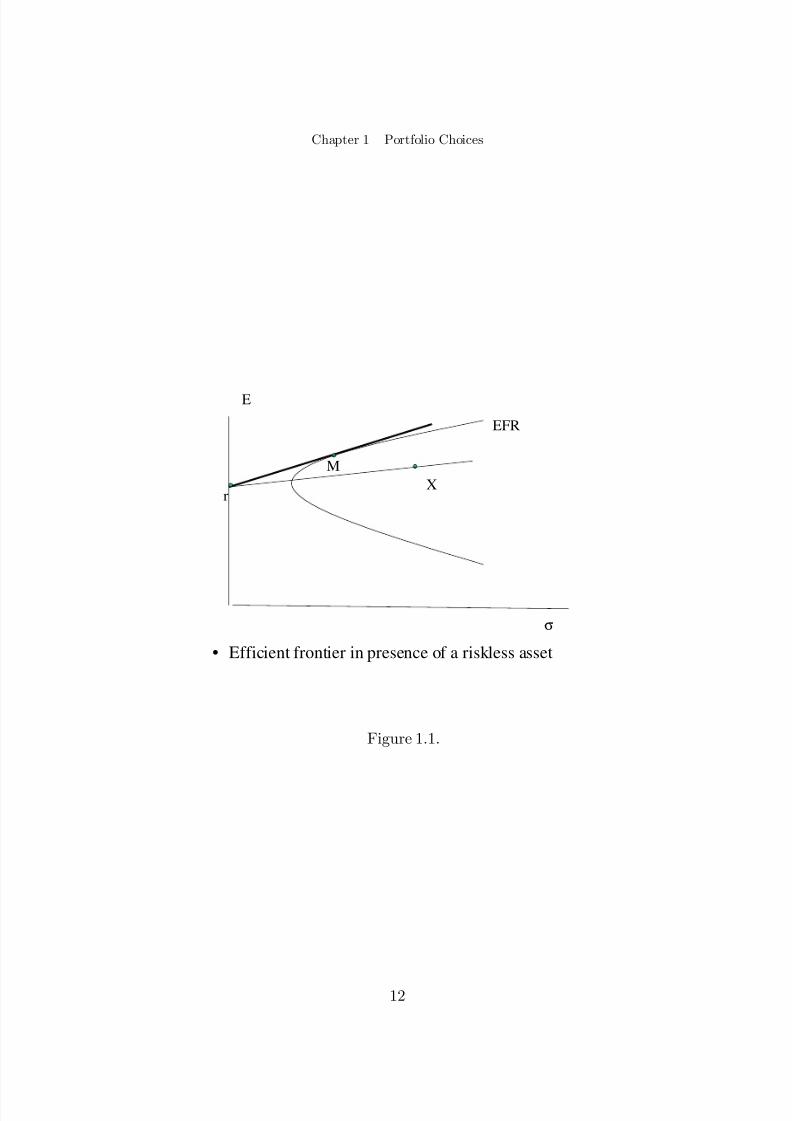
Consider Þ gure 1 where the upper branch of the hyperbola EFR represents, in the(σ , E ) space, the efficient portfolios in absence of a riskless asset. Assume now thatexists a risk free asset 0 yielding the certain return r. M stands for the tangencypoint of the hyperbola EFR with a straight line drown from r representing asset 0.Point M represents a portfolio composed only of risky assets, called the tangentportfolio.
11
8/3/2019 Capital Markets and Portfolio Theory, Roland Portait
http://slidepdf.com/reader/full/capital-markets-and-portfolio-theory-roland-portait 18/102
Chapter 1 Portfolio Choices
• Efficient frontier in presence of a riskless asset
σ
E
r
MX
EFR
Figure 1.1.
12
8/3/2019 Capital Markets and Portfolio Theory, Roland Portait
http://slidepdf.com/reader/full/capital-markets-and-portfolio-theory-roland-portait 19/102
Chapter 1 Portfolio Choices
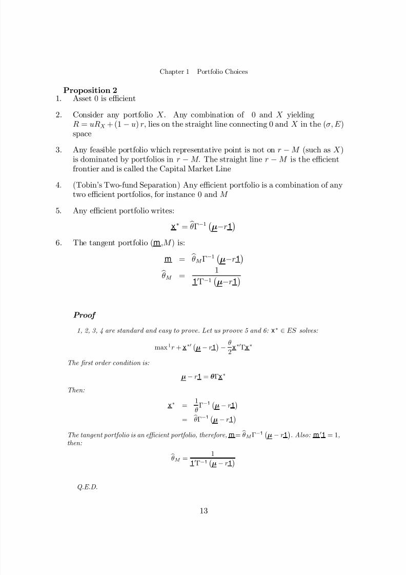
Proposition 2
1. Asset 0 is efficient2. Consider any portfolio X . Any combination of 0 and X yielding
R = uR X + (1 −u) r , lies on the straight line connecting 0 and X in the ( σ , E )space
3. Any feasible portfolio which representative point is not on r −M (such as X )is dominated by portfolios in r −M. The straight line r −M is the effi cientfrontier and is called the Capital Market Line
4. (Tobin’s Two-fund Separation ) Any effi cient portfolio is a combination of anytwo efficient portfolios, for instance 0 and M
5. Any efficient portfolio writes:
x∗ = bθΓ − 1¡µ −r 1¢6. The tangent portfolio (m ,M ) is:
m = bθM Γ− 1¡µ −r 1¢
bθM =1
10Γ − 1¡µ −r 1¢Proof
1, 2, 3, 4 are standard and easy to prove. Let us proove 5 and 6: x∗
∈ES solves:
max 1r + x∗0¡µ −r 1¢−θ2
x∗0Γ x∗
The Þ rst order condition is:
µ −r 1 = θ Γ x∗
Then:
x∗ =1
θΓ − 1
¡µ −r 1¢= bθΓ − 1¡µ −r 1¢The tangent portfolio is an e ffi cient portfolio, therefore, m = bθM Γ − 1 ¡µ −r1¢. Also: m 01 = 1 ,then:
bθM =1
10Γ − 1¡µ −r 1¢Q.E.D.
13
8/3/2019 Capital Markets and Portfolio Theory, Roland Portait
http://slidepdf.com/reader/full/capital-markets-and-portfolio-theory-roland-portait 20/102
Chapter 1 Portfolio Choices
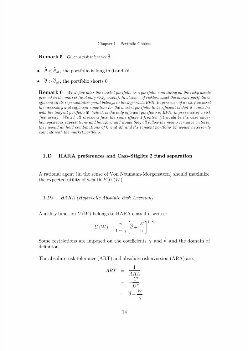
Remark 5 Given a risk tolerance
bθ:
• bθ < bθM , the portfolio is long in 0 and m
• bθ > bθM , the portfolio shorts 0
Remark 6 We de Þ ne later the market portfolio as a portfolio containing all the risky assets present in the market (and only risky assets). In absence of riskless asset the market portfolio is e ffi cient iif its representative point belongs to the hyperbola EFR. In presence of a risk free asset the necessary and su ffi cient condition for the market portfolio to be e ffi cient is that it coincides with the tangent portfolio m (which is the only e ffi cient portfolio of EFR, in presence of a risk free asset). Would all investors face the same e ffi cient frontier (it would be the case under
homogeneous expectations and horizon) and would they all follow the mean-variance criteria,they would all hold combinations of 0 and M and the tangent portfolio M would necessarily coincide with the market portfolio.
1.D HARA preferences and Cass-Stiglitz 2 fund separation
A rational agent (in the sense of Von Neumann-Morgenstern) should maximizethe expected utility of wealth E [U (W )].
1.D.i HARA (Hyperbolic Absolute Risk Aversion)
A utility function U (W ) belongs to HARA class if it writes:
U (W ) =γ
1 −γ · bθ +W γ ¸1− γ
Some restrictions are imposed on the coe fficients γ and
bθ and the domain of
deÞ nition.
The absolute risk tolerance (ART) and absolute risk aversion (ARA) are:
ART =1
ARA
= −U 0
U 00
=
bθ +
W γ
14
8/3/2019 Capital Markets and Portfolio Theory, Roland Portait
http://slidepdf.com/reader/full/capital-markets-and-portfolio-theory-roland-portait 21/102
Chapter 1 Portfolio Choices
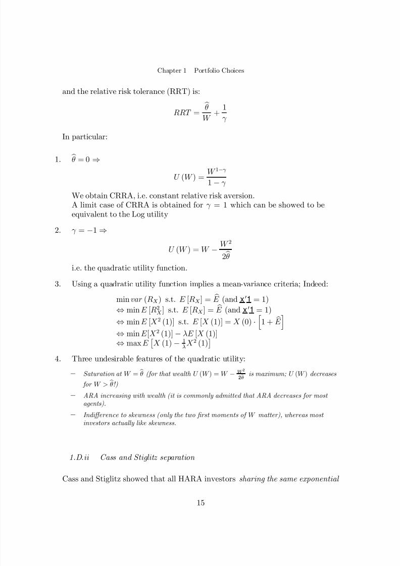
and the relative risk tolerance (RRT) is:
RRT = bθW +
1γ
In particular:
1. bθ = 0 ⇒U (W ) =
W 1− γ
1 −γ
We obtain CRRA, i.e. constant relative risk aversion.A limit case of CRRA is obtained for γ = 1 which can be showed to beequivalent to the Log utility
2. γ = −1⇒
U (W ) = W −W 2
2 bθi.e. the quadratic utility function.
3. Using a quadratic utility function implies a mean-variance criteria; Indeed:
min var (RX ) s.t. E [RX ] = bE (and x 01 = 1)
⇔min E [R2X ] s.t. E [RX ] = bE (and x 01 = 1)
⇔min E [X 2 (1)] s.t. E [X (1)] = X (0) ·h1 + bE i⇔min E [X 2 (1)] −λE [X (1)]
⇔max E £X (1) − 1λ X 2 (1)¤4. Three undesirable features of the quadratic utility:
— Saturation at W = bθ (for that wealth U (W ) = W −W 2
2 bθis maximum; U (W ) decreases
for W >
bθ!)
— ARA increasing with wealth (it is commonly admitted that ARA decreases for most agents).
— Indi ff erence to skewness (only the two Þ rst moments of W matter), whereas most investors actually like skewness.
1.D.ii Cass and Stiglitz separation
Cass and Stiglitz showed that all HARA investors sharing the same exponential
15

8/3/2019 Capital Markets and Portfolio Theory, Roland Portait
http://slidepdf.com/reader/full/capital-markets-and-portfolio-theory-roland-portait 22/102
Chapter 1 Portfolio Choices
parameter γ can build their optimal portfolios by mixing the two same funds.When a risk free asset exists it can be chosen as one of the two funds. Since allquadratic (mean-variance) investors exhibit the same γ (= −1) Tobin and Black2 fund separation are particular cases of Cass and Stiglitz separation. Cass andStiglitz conditions on the utility functions for separation to hold for investorssharing the same exponential parameter are summarized in the following table
Complete Market Incomplete Market @r (under complete markets ∃r ) quadratic or CRRA 2
∃r class wider than HARA HARA
2 in the particular case of CRRA one fund su ffi ces (for a given γ the portfolio is the same for all W
16
8/3/2019 Capital Markets and Portfolio Theory, Roland Portait
http://slidepdf.com/reader/full/capital-markets-and-portfolio-theory-roland-portait 23/102
Chapter 2 Capital Market Equilibrium
Chapter 2Capital Market Equilibrium
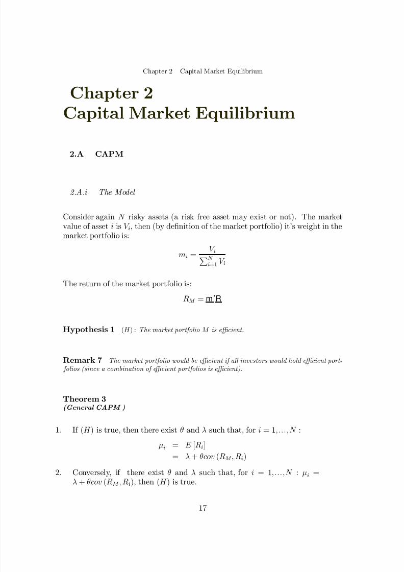
2.A CAPM
2.A.i The Model
Consider again N risky assets (a risk free asset may exist or not). The marketvalue of asset i is V i , then (by de Þ nition of the market portfolio) it’s weight in themarket portfolio is:
m i =V i
PN i=1 V i
The return of the market portfolio is:
RM = m0
R
Hypothesis 1 (H ) : The market portfolio M is e ffi cient.
Remark 7 The market portfolio would be e ffi cient if all investors would hold e ffi cient port- folios (since a combination of e ffi cient portfolios is e ffi cient).
Theorem 3(General CAPM )
1. If (H ) is true, then there exist θ and λ such that, for i = 1 ,...,N :
µi = E [R i ]= λ + θcov (RM , R i )
2. Conversely, if there exist θ and λ such that, for i = 1 ,...,N : µi =λ + θcov (RM , R i), then (H ) is true.
17
8/3/2019 Capital Markets and Portfolio Theory, Roland Portait
http://slidepdf.com/reader/full/capital-markets-and-portfolio-theory-roland-portait 24/102
Chapter 2 Capital Market Equilibrium
Proof
The proof comes directly from Theorem 1.
Q.E.D.
Remark 8 θ can be interpreted as the risk aversion of the average (representative) investor.
Remark 9 CAPM holds for any portfolio ( x , X ).
Indeed, call RX its return and consider the case where no risk free asset exists(x01 = 1) :
E [RX ] =N
Xi=1
xi µi
=N
Xi=1
xi (λ + θcov (RM , R i ))
=N
Xi=1
xi λ + θN
Xi=1
x i cov (RM , R i)
= λ + θcovÃRM ,
N
Xi=1x iR i
!= λ + θcov (RM , R X )
Remark 10 The proof follows the same lines when the portfolio contains a risk free asset with weight x0
Remark 11 λ and θ are the same for all assets or portfolios
Remark 12 For the market portfolio:
µM = λ + θcov (RM , RM )= λ + θσ 2
M
Therefore:
θ =µM −λ
σ 2M
Then:
µi = λ + θcov (RM , R i )
= λ + ·µM −λσ 2
M ¸cov (RM , R i )
18
8/3/2019 Capital Markets and Portfolio Theory, Roland Portait
http://slidepdf.com/reader/full/capital-markets-and-portfolio-theory-roland-portait 25/102
Chapter 2 Capital Market Equilibrium
De Þ ne:
β i =cov (RM , R i )
σ 2M
Then we may write the CAPM equation in the alternative form:
E [R i ] = λ + β i (µM −λ )
Consider any portfolio z with β Z = 0 :
β Z = 0
⇔ cov (RM , RZ ) = 0
⇔ cov (m0
R , z0
R ) = z0Γ m = 0
⇐⇒z⊥Γ m
⇔ z∈[vect (Γ m )]⊥
vect [v 1, v 2, ..., v N ] is the set of all linear combinations of v 1, v 2, ..., v N , or linearsubspace generated by v 1, v 2, ..., v N . The dimension of [vect (Γ m )]⊥ is thus N −1and there are an in Þ nity of 0-beta portfolios. Now, from the general CAPM, wewould have: λ = µZ ; Thus:
Corollary 1 ( 0−beta CAPM) If M is e ffi cient, for any zero beta portfolio or asset Z : E [R i ] =µZ + β i (µM
−µZ )
Corollary 2 (Standard CAPM ) : If there exists a risk-free asset yielding r (which is a par-ticular zero beta asset)
E [R i ] = r + β i (µM −r )
Note that µZ = r for any zero beta portfolio or asset.
2.A.ii Geometry
missing
2.A.iii CAPM as a Pricing and Equilibrium Model
• For a security delivering eV (1) at time 1(the pdf of eV (1) is given, thusE (
eV (1)) and cov(
eV (1) , RM ) are known), what is its price V (0) at time 0?
19
8/3/2019 Capital Markets and Portfolio Theory, Roland Portait
http://slidepdf.com/reader/full/capital-markets-and-portfolio-theory-roland-portait 26/102
Chapter 2 Capital Market Equilibrium
Let’s assume that there exists a risk-free asset, then:
E heV (1)iV (0)= E [1 + R] = 1 + r + θcovÃeV (1)
V (0), R M !
with
θ =µM −r
σ2M
Then:
E heV (1)i= (1 + r ) V (0) + θcov³eV (1) , RM
´and
V (0) =E heV (1)i−θcov³eV (1) , R M ´1 + r
i.e. V (0) is the present value of its certainty equivalent at time 1 discountedat the risk-free rate.However this asset may be an element of the market portfolio M (unless thisclaim is in zero net supply ..) and therefore the previous pricing formula isnot a closed form general equilibrium relation.
• In fact CAPM is an equilibrium condition stemming from the demand side;The equilibrium price can only be otained by specifying the supply side (inthe previous example the supply was a right on an exogeneous cash ß ow X ).General equilibrium requires a speci Þ cation of the supply of all securitiestraded in the market.
— Consider the N risky assets together and we look for their equilibrium prices. We assume Þ rst an inelastic supply. Assume that asset i delivers
eV i (1 ), an exogenous cash
ß ow, at time 1 , what is its price at time 0?
E heV i (1 )iV i (0)= 1 + r + ·µM −r
σ 2M ¸covÃeV i (1 )
V i (0), RM !
For i = 1 , 2,...,N . We have N equations with N unknowns V i (0) ( i = 1 ,...,N ).( 1 + RM = PN
i = 1 eV i (1)
PN i = 1 V i (0) allows to compute µM , σ 2
M ,cov³eV i (1)V i (0) , R M ´as functions of the
V i (0))
— Consider again the N risky assets and an elastic supply with constant returns to scale,where the joint pdf of the R i is given and independent of the scale V i (0) to be invested in ”technology i”. The CAPM determines the scale V i (0) of investment in technology i
20
8/3/2019 Capital Markets and Portfolio Theory, Roland Portait
http://slidepdf.com/reader/full/capital-markets-and-portfolio-theory-roland-portait 27/102
Chapter 2 Capital Market Equilibrium
by the equations:
µi = E [R i ] = r + ·µM −rσ2
M ¸cov (RM , R i )
and
1 + RM = PN i = 1 V i (0) · (1 + R i )
PN i = 1 V i (0)
2.A.iv Testing the CAPM
One remark about this important empirical topic.Testing the CAPM is equivalent to testing (H ). However, how should we de Þ nethe market portfolio and how to measure the market return?Usually the market portfolio is proxied by stock (plus bond) indices. But resultson stock indices do not include all assets in M (non tradable assets, art,..). Hencewe test the e fficiency of the index and not that of M (Roll’s Critique).
2.B Factor Models and APT
2.B.i K -factor models
Hypothesis 2 There exist K factors, F k , k = 1 , 2,...K with
1. F i⊥F j
2. E [F k ] = 0
3. var (F k ) = σ2k
such that for i = 1 , 2,...,N :
R i = µi +K
Xk = 1
β ik F k + ² i
where E [² i ] = 0 and ² i ⊥² j ⊥F k . In vector form:
R N × 1 = µ + β N × K F K × 1 + ² = µ +K
Xk = 1
β 0k F k + ²
21
8/3/2019 Capital Markets and Portfolio Theory, Roland Portait
http://slidepdf.com/reader/full/capital-markets-and-portfolio-theory-roland-portait 28/102
Chapter 2 Capital Market Equilibrium
with β k being the kth row of β .
• In practice, we should have large N and small K , so that in estimating thevariance-covariance matrix,
cov (R i , R j ) =K
Xk =1
β ik β jk σ2k
we only need to estimate K terms of σ2k and run N regressions for estimating
the β ik
.
• In CAPM or in the Markowitz model, without the factor decomposition, weneed to estimate N (N −1) / 2 terms.
• A Particular case: K = 1 boils down into the market model that writes:
R i = µi + β iF + ² i
Then:
RM =N
Xi=1
m i µi + F N
Xi=1
m i β i +N
Xi=1
m i ² i
= µM + F
Since the innovation terms diversify and β M = PN i=1 m i β i = 1 :
F = RM −µM
and
R i = µi + β i [RM −µM ] + ² i
Note that the R i are linked through [RM −µM ] (since cov (R i , R j ) = β i β j σ2M ).Also, β i [RM −µM ] is the systematic risk, and ² i is the unsystematic (diversi Þ able)risk; only systematic risk should be priced (CAPM).
2.B.ii APT
We assume that the returns are generated by a K factors linear process previouslydeÞ ned that writes:
22
8/3/2019 Capital Markets and Portfolio Theory, Roland Portait
http://slidepdf.com/reader/full/capital-markets-and-portfolio-theory-roland-portait 29/102
Chapter 2 Capital Market Equilibrium
R = µ + + β F + ² = µ +K
Xk =1
βkF k + ²
Recall that βk
is an N dimensioned column vector with an i th component equalto β ik
De Þ nition 4 A zero investment portfolio, de Þ ned by the amount of wealth, x , invested in each asset, satis Þ es:
x 01 = 0
V (0) = 0V (1 ) = x 0R
The last equation can be veri Þ ed since:
V (1) =N
Xi=1
xi (1 + R i ) =N
Xi=1
xi +N
Xi=1
x iR i = x 0R
De Þ nition 5 An arbitrage portfolio is a zero investment portfolio with x 0R ≥ 0 almost
surely and E [x0R ] > 0.Absence of arbitrage (AOA) prevails if no arbitrage portfolio can be constructedi.e:x01 = 0 and x0R ≥0 a.s. implies x0R = 0 a.s. (or equivalently implies E (x0R ) =0)
Theorem 4(APT ) In AoA there exist K + 1 scalars such that:
µ = λ 0 1 + λ 1β1 + ... + λ K β K
or µi = λ 0 + λ 1 β i 1 + ... + λ K β iK
• λ 0 is the required rate of return without systematic risk.
• λ k is the market price of risk k.
• λ k β ik is the risk premium imposed to security i because it has a risk k of intensity β ik .
23
8/3/2019 Capital Markets and Portfolio Theory, Roland Portait
http://slidepdf.com/reader/full/capital-markets-and-portfolio-theory-roland-portait 30/102
Chapter 2 Capital Market Equilibrium
Proof
Consider any well-diversi Þ ed zero investment portfolio satisfying:
x 01 = 0 or x⊥1x0β k = 0 or x⊥
βk for k = 1 ,...,K
hence:
x is any element of hvect³1 ,β 1 , β2 ,..., β
K ´i⊥Also x0² = 0 (since it is well diversi Þ ed); Then:
RX = x 0R
= x 0µ +
K
Xk = 1
F k x 0βk + x 0
²
= x 0µ
Since x 0µ is certain, in AoA x 0µ must be zero (if x 0µ > 0 then x is an arbitrage portfolioand if x 0µ < 0 then −x is an arbitrage portfolio). Thus: x0µ = 0 or x⊥µ , which means that µ is orthogonal to any element x of [vect(1 , β 1 , β 2 ,..., β K )]
⊥ , i.e.
µ∈vect(1 , β 1 , β 2 ,..., β K )
implying that exist K + 1 scalars such that : µ = λ 0 1 + λ 1β 1 + ... + λ K β K
Q.E.D.
• In the particular case where there is a risk-free asset, then:
µ0 = λ 0 = r
and
µi = r + λ 1β i1 + ... + λ K β iK
2.B.iii Arbitrage and Equilibrium
• Equilibrium implies AoA, but the inverse is not true.
• AoA conditions do not involve utility functions.
24

8/3/2019 Capital Markets and Portfolio Theory, Roland Portait
http://slidepdf.com/reader/full/capital-markets-and-portfolio-theory-roland-portait 31/102
Chapter 2 Capital Market Equilibrium
2.B.iv References
Dumas-Allaz, 1995 ; Demange-Rochet, 1992.
25
8/3/2019 Capital Markets and Portfolio Theory, Roland Portait
http://slidepdf.com/reader/full/capital-markets-and-portfolio-theory-roland-portait 32/102
PART IIMultiperiod CapitalMarket Theory : the
Probabilistic Approach
8/3/2019 Capital Markets and Portfolio Theory, Roland Portait
http://slidepdf.com/reader/full/capital-markets-and-portfolio-theory-roland-portait 33/102
Chapter 3 Framework
Chapter 3Framework
3.A Probability Space and Information
We consider the usual probability triplet (Ω , F , P ), where F is a σ-algebra on Ω
representing the observable events at time T .
Information in the period [0, T ] is represented by a Þ ltration F t t∈[0,T ], where F tis the set of observable events at time t (represented by a σ−algebra), and thesequence F t t∈[0,T ] satis Þ es the ”usual” conditions:
F 0 = null events and a.s. event (s < t ) ⇔ (F s⊂F t )
F T = F F s = \t>s
F t
In the discrete time setting, all transactions take place at discrete points, i.e.,t = 1 , 2,...,T . In the continuous time setting, transactions take place continuously,i.e., t∈[0, T ].
We assume a frictionless market, continuously open in the continuous time frame-work.
27
8/3/2019 Capital Markets and Portfolio Theory, Roland Portait
http://slidepdf.com/reader/full/capital-markets-and-portfolio-theory-roland-portait 34/102
Chapter 3 Framework
3.B Asset Prices
3.B.i De Þ nitions and Notations
There are N + 1 assets traded in the market, one being the locally risk-free as-set, denoted by 0, and the remaining N being the risky assets. The prices of those assets are noted S i (t) ( for i = 0 , 1,...,N ); S(t) = ( S 1(t), . . ,S N (t))0 or(S 0(t), S 1(t), . . ,S N (t))0 (depending on the context) is the N (or N + 1 ) dimen-
sional column vector of asset prices. Without loss of generality it will generallybe assumed that S i (0) = 1It is assumed for the time being that there is no dividend, or that a dividend isreinvested in the asset that delivers it.1. In the discrete time case S 0(t) = S 0(t −1)[1 + r (t −1)], with r (t −1) beingthe locally risk-free rate in [t −1, t] , known at time t −1 but unknown before.Remark that S 0(t + 1) = S 0(t)(1+ r (t)) is random at t −1 since r (t) is unknown.2. In the continuous time context:
• r (t) is stochastic but F t -adapted.
For a risk-free asset:
dS 0 = S 0rdt
or
S 0 (t) = eR t0 r (u )du
with S 0 (0) = 1 .
• For a risky asset we will usually assume that prices follow Ito processes:dS i = S i µidt + S i σ i
0dw
with risk induced by w , the vector of standard Brownian Motions.
Technical conditions (e.g., the integrability conditions) apply.If S i follows Ito process, we preclude jumps. If jumps are involved, however, thena rather general assumtion is that S i follows a semi-martingale process. A slightlymore speci Þ c assumption is that asset prices follow processes that yield a.s. RightContinuous and Left Limited (RCLL) paths. When considering the possibility of
28
8/3/2019 Capital Markets and Portfolio Theory, Roland Portait
http://slidepdf.com/reader/full/capital-markets-and-portfolio-theory-roland-portait 35/102
Chapter 3 Framework
jumps we will assume RCLL processes for the asset prices to avoid the so Þ sticationof semi martingales 3.
• It is worthwhile to note that Ito processes ⊂RCLL ⊂Semi −martingales .
• Most of the results of the next chapter (On AOA and completeness) hold inthe semi-martingale case.
3.C Portfolio Strategies
3.C.i Notation:
• n (N +1) × 1 the vector of the N+1 numbers of assets ; xN × 1 the vector of N weights on risky assets
• S (N +1) × 1 the vector of the N+1 asset prices
• X (t) = n 0(t)S(t) the value of the portfolio at t
• (n ,X ) or (x ,X ) a strategy
3.C.ii Discrete Time
[t −1, t[ is period t −1;at time t S (t) is set and, just after, n(t) is choosen
• During period t −1, the value of the portfolio will evolve:X (t) −X (t −1) = n 0(t)S(t)−n 0(t −1)S(t −1)
= n 0(t −1) [S(t) −S(t−1)] + S0(t) [n (t) −n (t −1)]
The Þ rst term in the right hand side of the equation, n 0(t −1) [S(t) −S(t−1)], isthe gain during the period [t −1, t[ , and is represented as g(t −1, t).3 Consider the integral: R φ (u ) dS . In a regular integral of this form dS is inÞ nitesmal, while in a
jump process it can assume some Þ nite value somewhere.
29
8/3/2019 Capital Markets and Portfolio Theory, Roland Portait
http://slidepdf.com/reader/full/capital-markets-and-portfolio-theory-roland-portait 36/102
Chapter 3 Framework
The second term can be deemed as the net cash in ß ow added to the portfolio attime t. Indeed it can be decomposed into two terms: −S0(t)n (t −1), the value of assets sold at time t, and S0(t)n (t), the algebric value of assets purchased (maybe < 0 if sales> purchases).
• The cumulative gain in [0, t], deÞ ned for t = 1 ,...,T , can be represented as:
G(t) =t
Xu =1
g(u −1, 1)
De Þ nition 6 (Self- Þ nancing Portfolio ) When at each time t the net in ß ow is 0, the strategy is said to be self- Þ nancing, i.e., if (n ,X ) is self- Þ nancing, then:
X (t) −X (t −1 ) = g(t −1 , t ) = n 0(t −1 ) [S (t) −S(t−1)]
and
X (t) = X (0) + G(t)
• Let S i (t) be the value of asset i at time t, and S 0(t) be the numeraire, thenthe discounted value of i is:
S di =S i (t)S 0(t)
• Self-Þ nancing is independent of the numeraire used; In particular (n ,X )self-Þ nancing implies:
X d(t) −X d (t −1) = n 0(t −1)£Sd (t) −S d (t −1)¤3.C.iii Continuous Time
• The gain process in [t, t + dt) is deÞ ned as:
dG(t) = n 0(t)dS(t)
and
G(t) = Z t
0dG(u) = Z t
0n 0(u)dS(u)
30

8/3/2019 Capital Markets and Portfolio Theory, Roland Portait
http://slidepdf.com/reader/full/capital-markets-and-portfolio-theory-roland-portait 37/102
Chapter 3 Framework
• The change of the portfolio value is found to be:
dX = d (n 0(t)dS(t))= n 0(t)dS(t)+ S0(t)dn 0(t)+ dn 0(t)dS(t)= n 0(t)dS(t)+ dn 0(t) [S(t)+ dS(t)]
with the Þ rst term in the right hand side of the equation being the period gaindG(t) and the second term the net in ß ow at t + dt.
• Again, in a self- Þ nancing strategy: dX (t) = dG(t), and X (t) = X (0) + G(t);As in the discrete time case, the self Þ nancing property as well as theexpression of the gain do not depend on the choosen numeraire .
31

8/3/2019 Capital Markets and Portfolio Theory, Roland Portait
http://slidepdf.com/reader/full/capital-markets-and-portfolio-theory-roland-portait 38/102
Chapter 4 AoA, Attainability and Completeness
Chapter 4AoA, Attainability andCompleteness
4.A De Þ nitions
De Þ nition 7 strategy (n ,X ) is admissible if:
1. n (t) is F t adapted and satis Þ es some technical conditions 4.
2. X (t)∈L1,2.
3. (This is an additional condition imposed sometimes) X (t) is bounded frombelow to avoid doubling Strategies 5 .
De Þ nition 8 A is the set of admissible strategies
De Þ nition 9 A0 = Self- Þ nancing and admissible strategies
We now work with A0, i.e., ∀(n ,X )∈A0, dX = n 0dS .4 Technical conditions on n ( t ) :
, when asset prices follow RCLL processes(a) G(t) = R t
0 n 0(u)dS(u) must be de Þ ned for S(t)∼RCLL
(b) (Integrability )
i.
R t
0 kn 0(u)k2 du< ∞a.s.
ii. R t
0 |n0(u)| du< ∞a.s.
(c) (predictability of n (t))n (t)∼LCRL so that if there is a jump in S(t), rebalancing must takeplace in t+ but never in t− , the latter being equivalent to insider trading,i.e., a rebalancing, or jump, in n (t) takes the advantage of a jump in S(t)that has just occured. This condition is not necessary when S(t) iscontinuous.
5 In a Doubling Strategy the gambler bets 2 when losing 1 and bets 4 when losing 2...
32
8/3/2019 Capital Markets and Portfolio Theory, Roland Portait
http://slidepdf.com/reader/full/capital-markets-and-portfolio-theory-roland-portait 39/102
Chapter 4 AoA, Attainability and Completeness
It is also possible to de Þ ne a strategy by a vector of weights x N × 1. The weight of the risk-free asset in the portfolio is then 1 −x01 .
De Þ nition 10 (a ,A) is an arbitrage if:
1. (a ,A)∈A0.
2. A(0) = n 0(0)S(0) =0 , (i.e., zero initial investment).
3. A(T ) ≥0 a.s. (i.e., non-negative cash ß ow at the end).
4. E [A(T )|F 0] > 0
There is an arbitrage opportunity each time that a strategy (x, X ) in A0 dominatesanother strategy (y, Y ) in A0 (i.e. X (T ) ≥Y (T ) a.s. and E [X (T )] ≥E [Y (T )] forthe same initial investment X (0) = Y (0); or X (T ) = Y (T ) a.s. with X (0) < Y (0)).Arbitrage is built by being long in (x, X ) and short in (y, Y ).
Example 1 X (T ) ≥S 0 (T ) = eR T
0 r ( u )du a.s. ; E (X (T ) −S 0 (T )) > 0 and X (0) = 1
Example 2 X (T ) = K , a constant, while X (0) < KB T (0) where BT (0) denotes the value
at time 0 of a zero-coupon bond yielding 1 at time T.
The previous considerations imply:
Proposition 3In AoA, all self- Þ nancing and admissible portfolios yielding a.s. the same terminal value must require the same initial investment, i.e. ∀(x ,X ) ∈A0 and ∀¡y ,Y ¢∈A0
with X (T ) = Y (T ) a.s. , then in AoA: X (0) = Y (0).
DeÞ
nition 11 eC T is a contingent claim if
1. eC T is F T measurable.
2. eC T ∈L1,2 (Þ nite mean and variance).
3. (goes with hypothesis on admissible strategies) eC T is bounded from below.
De Þ nition 12 C , the set of contingent claims
33

8/3/2019 Capital Markets and Portfolio Theory, Roland Portait
http://slidepdf.com/reader/full/capital-markets-and-portfolio-theory-roland-portait 40/102
Chapter 4 AoA, Attainability and Completeness
Example 3 The terminal values of N + 1 primitive assets are contingent claims.
Example 4 ∀A∈F T , the indicator function 1 A is a contingent claim.
De Þ nition 13 eC T ∈C is attainable if ∃(c ,C )∈A0 with C (T ) = eC T a.s. . We say eC T is
attained by (c,C ) or (c,C ) yields eC T .
De Þ nition 14 Ca = attainable contingent claims
De Þ nition 15 Cn = non-attainable contingent claims
De Þ nition 16 The market is (dynamically) complete when all contingent claims are attain-able, i.e., Ca = C or Cn = ∅.
Remark 13 Market completeness is unrealistic in discrete time, but less unrealistic in con-tinuous time. In continuous time the possibility of rebalancing at each point of time allows a much larger spanning. When completeness is obtained through continuous rebalancing, the market is said “dynamically” complete.
De Þ nition 17 A pricing formula π maps C onto R. To be viable, π must satisfy:
1. π is linear, i.e., ∀λ 1, λ 2, eC T ∈C, and eC 0T ∈
C:
π ³λ 1eC T + λ 2eC 0T ´= λ 1π ³eC T ´+ λ 2π³eC 0T ´2. ∀eC T ∈
C
(a)
eC T ≥0 a.s. ⇒π³
eC T ≥0
(b) eC T = 0 a.s. ⇒π
³eC T
´= 03. (Viability or Compatibility Condition) ∀(x ,X ) attaining eC T (i.e., X (T ) = eC T
a.s. ):
π³eC T ´= X (0)
De Þ nition 18 Π = π |π viable
34

8/3/2019 Capital Markets and Portfolio Theory, Roland Portait
http://slidepdf.com/reader/full/capital-markets-and-portfolio-theory-roland-portait 41/102
Chapter 4 AoA, Attainability and Completeness
De Þ nition 19 Two probability measures P and Q are equivalent if they have the same null sets (the impossible as well as the certain events are the same for P and Q)
De Þ nition 20 An adapted stochastic process is a martingale if at each point of time the (conditional) expectation of a future value is the current value i.e:
Z (t) is a martingale if E [Z (t)/F s ] = Z (s) for any s and t such that 0 ≤s ≤ t ≤T
De Þ nition 21 Q = nQ|Q∼P and ∀(x ,X )∈A0, E Q hX (T )S 0 (T ) |F 0i= X (0 )
S 0 (0) o. Equivalently,Q is a set of P -equivalent probability measures Q under which the asset 0 discounted asset prices X d (T ) = X ( T )
S 0 ( T ) are martingales.
It should be noted that X (0) 6= E P
hX (T )S 0 (T ) |F 0ibecause investors are risk-averse
and expect a return di ff erent than the risk-free rate r (usually higher since, ingeneral, holding a risky asset increases the risk of their portfolio). However, thisdoes not mean that there is no such a probability measure as Q that yields Q-martingale discounted prices.
In the following we will consider the problems:
• Are Q and Π empty?
• What is the relation between Q and Π ?
4.B Propositions on AoA and Completeness
Recall in the following that S 0 (0) = 1
4.B.i Correspondance between Q and Π : Main Results
Theorem 5Assume Q and Π are not empty. There exists a one-to-one relation between Q and Π .
• Q →π Q , deÞ ned by:
∀eC T ∈C : π Q ³eC T ´= E Q "eC T
S 0 (T )|F 0#
35
8/3/2019 Capital Markets and Portfolio Theory, Roland Portait
http://slidepdf.com/reader/full/capital-markets-and-portfolio-theory-roland-portait 42/102
Chapter 4 AoA, Attainability and Completeness
• π
→Qπ , deÞ ned by:
∀A∈F T : Qπ (A) = E Q [1A ] = π (1A · S 0 (T ))
Proof
Let us begin by showing that π Q is a viable pricing system. Indeed:
1. π Q is linear (because the expectation operator E is linear), i.e., ∀
eX T ∈
Ca
and ∀
eY T ∈
Ca :
π Q ³λ eX T + µeY T ´ = E Q "λ eX T + µeY T
S 0 (T ) #= E Q "λ eX T
S 0 (T )#+ E Q "µeY T
S 0 (T )#= λπ Q ³eX T ´+ µπ Q ³eY T ´
2. ∀
eC T ≥0 a.s. , π Q ³
eC T ≥0;Indeed:
eC T > 0⇒π Q ³eC T ´= E Q "eC T
S 0 (T )#> 0
and
eC T = 0 a.s.⇒π Q ³eC T ´= E Q "eC T
S 0 (T )#= 0
3. (Compatibility Condition) ∀(x ,X ) attaining
eC T , i.e., X (T ) =
eC T a.s. .,
π Q
³eC T
´= X (0); Indeed:
π Q ³eC T ´ = E Q "eC T
S 0 (T )#= E Q ·X (T )
S 0 (T )¸= E Q £X d(T )|F 0¤= X (0)
since Q yields martingale discounted prices
36
8/3/2019 Capital Markets and Portfolio Theory, Roland Portait
http://slidepdf.com/reader/full/capital-markets-and-portfolio-theory-roland-portait 43/102
Chapter 4 AoA, Attainability and Completeness
4. It has been shown that π Q is a viable pricing formula that maps Q into Π .Moreover, this mapping is injective, i.e., ∀Q
0 6= Q and Q0, Q∈Q, π Q 0 6= π Q .Indeed:
Q0 6= Q
⇒ ∃A∈F T s.t. Q0(A) 6= Q (A)
⇐⇒E Q0
[1A ] 6= E Q [1A ]
Consider a contingent claim 1A S 0 (T ):
π Q (1A S 0 (T )) = E Q
·1A S 0 (T )
S 0 (T )
¸= E Q [1A ]
and
π Q 0 (1A S 0 (T )) = E Q0 ·1A S 0 (T )
S 0 (T ) ¸= E Q
0
[1A ]
Therefore we obtain di ff erent prices for this particular contingent claim,hence, π Q 0 6= π Q .
5. The proof ends by checking that when π is a viable price systemQ (A) = π (1A · S 0 (T )) deÞ nes a probability measure which has the samenull sets than P .
Q.E.D.
Corollary 3 Q = ∅⇐⇒π = ∅
Corollary 4 Q is a singleton
⇐⇒
π is a singleton
Theorem 61. In AoA, a viable pricing formula on Ca exists and is unique.
2. Market is complete and AOA ⇐⇒Q is a singleton ⇐⇒
Π is a singleton
3. AoA⇐⇒Q 6= ∅⇐⇒
Π 6= ∅Proof :
37
8/3/2019 Capital Markets and Portfolio Theory, Roland Portait
http://slidepdf.com/reader/full/capital-markets-and-portfolio-theory-roland-portait 44/102
Chapter 4 AoA, Attainability and Completeness
1. Assume AoA and consider any
eC T
∈
Ca attained by (x ,X ). Because thecompatibility condition it is only possible to de Þ ne the price of eC T by π³eC T ´=
X (0). If another strategy ¡y ,Y ¢attains fC T , X (0) = Y (0) because AOA, Hencethere is only one viable pricing of an attainable claim under AOA.2. Under AOA, if the market is complete all claims are attainable, hence there isone and only one viable price for any contingent claim in C .3. Under AOA and incomplete markets there are an in Þ nite number of viableprices for a non-attainable contingent claim ( Π 6= ∅but is not a singleton). WhenAOA does not prevail no pricing system meets the compatibility condition, henceΠ is empty.
4.B.ii Extensions
4.B.ii.a Extension I.
Consider eC T ∈Ca attained by (x ,X ) and consider Q∈
Q:
• — At time 0, π³eC T ´= E Q heC T
S 0 ( T ) |F 0i· S 0 (0) = E Q heC T
S 0 ( T ) |F 0i= X (0)
— At time s∈[0, T ]:
π s ³eC T ´ = E Q ·X (T )S 0 (T )
|F s¸· S 0 (s)
=X (s)S 0 (s)
· S 0 (s)
= X (s)
4.B.ii.b Extension II.
The portfolio is not self-Þ
nancing:
• — Assume an adapted and integrable dividend payment δ (t) in [t, t + dt], then:
X (0) = E Q0 (Z T
0 hδ (t) e− R t
0 r ( u ) du idt + X (T ) e− R T
0 r ( u ) du ) — Assume a cumulative dividend stream dD (t) in [t, t + dt], then:
X (0) = E Q0 (Z T
0 hdD (t) e− R t
0 r (u )du idt + X (T ) e− R T
0 r ( u ) du )38
8/3/2019 Capital Markets and Portfolio Theory, Roland Portait
http://slidepdf.com/reader/full/capital-markets-and-portfolio-theory-roland-portait 45/102
Chapter 5 Alternative Speci Þ cations of Asset Prices
Chapter 5Alternative Speci Þ cations of AssetPrices
5.A Ito Process
There are N + 1 assets in the market:
• r (t) being the adapted, locally risk-free rate, asset 0 is the correspondingrisk-free asset with:
dr = α r (t) dt + σ 0r (t) dw
dS 0 (t) = S 0 (t) r (t) dt⇔S 0 (t) = eR t0 r (u )du
At t : dr (t) is not known, but dS 0 is known.
• The N risky assets follow the process:
dS = α (t) dt + Ω (t) dw
⇔ S (t) = S (0) + Z t
0α (u) du + Z t
0Ω (u) dw
or for the i th asset
dS i= α i (t) dt + Ω 0i (t) dw
where w M × 1 is the vector of standard Brownian Motions and α N × 1 (t) andΩ
N × M (t) are the two adapted processesΩ 0
i is the ith
row of Ω
. The coeffi
cientsof all these Ito processes are stochastic processes that satisfy integrabilityconditions.
• In terms of returns:
dR i =dS iS i
= µi (·) dt + σ 0i (·) dw
or in vector form:
dR = µ (·) dt+ Σ (·) dw
39
8/3/2019 Capital Markets and Portfolio Theory, Roland Portait
http://slidepdf.com/reader/full/capital-markets-and-portfolio-theory-roland-portait 46/102
Chapter 5 Alternative Speci Þ cations of Asset Prices
where σ 0i is the ith row of Σ , the diff usion matrix.
Equivalently:
S i (t) = S i (0) eR t0 [µ i (.)− 1
2 kσ i (.)k2 ]du +R t0 σ 0
i ( .)dw
The integrability conditions on the coe fficients are:(IC ) R t
0 |µi(.)| du and R t0 kσ i (.)k
2 du deÞ ned a.s fori = 1 ,...,N They will be refered as the integrability conditions (IC ) in the followingchapters
• Ito process yields continuous sample paths, but they are not necessarily
Markovian.
5.B Di ff usions
• S(t) follows a diff usion process if:
dS = α (t, S (t) , r (t)) dt + Ω (t, S (t) , r (t)) dw
or
dS i= α i (t, S (t) , r (t)) dt + Ω 0i (t, S i (t) , r (t)) dw
or
dR = µ (t, S (t) , r (t)) dt+ Σ (t, S (t) , r (t)) dw
or, equivalently
S i (t) = S i (0) eR t0 [µ i − 1
2 kσ i k2 ]du +R t0 σ 0
i dw
The process for the risk-free rate is:
dr = µr (t,r, S) dt + σ0r (t,r, S) dw
with the coe fficients ( α (·) , µ (·) , Ω (·) , ..), being a deterministic function of stochastic variables r, S and the deterministic t.
• The di ff usion process is an Ito process, hence it exhibits continuous samplepaths. Moreover it is Markovian since the next increment depends on t andS(t) , r (t) only.
• Technical conditions to be satis Þ ed bythe coefficients of a diff usion process arethe Lipschitz condition and the linear growth condition.
40
8/3/2019 Capital Markets and Portfolio Theory, Roland Portait
http://slidepdf.com/reader/full/capital-markets-and-portfolio-theory-roland-portait 47/102
Chapter 5 Alternative Speci Þ cations of Asset Prices
5.C Di ff usion state variables
The state of the economy is de Þ ned by L state variables Y obeying the di ff usionSDE: dY = α Y (t, Y (t)) dt + Ω Y (t, Y (t)) dw(the coefficients meet the integrability conditions). The dynamics of all the Þ nan-cial variables depend on (t, Y (t)) ,i.e:dR = µ (t, Y (t)) dt+ Σ (t, Y (t)) dw ; dr = µr (t, Y ) dt + σ0
r (t, Y ) dwRemark that- The processes are Markovian- The simple di ff usion case is a particular case of the state variable di ff usion case(where S and r are the state variables); the state variable di ff usion case is aparticular case of the Ito case.
5.D Theory in the Ito-Di ff usion Case
All the results on AOA, martingale measures, viable prices, completeness,.., pre-sented in the case of RCLL asset prices and LCRL strategies hold of course whenthey follow Ito or di ff usion processes (which are continuous). We present in thefollowing some speciÞ c results valid in these last cases.
5.D.i Framework
• Assume the usual probability triplet [Ω , F , P ] .
• Let w M × 1 denote the sources of uncertainties. The observable eventsat t are the events w (t0) ≤ a for all t0 ≤ t and all the real vectors a:roughly, information at t is represented by the path of w between 0 andt. F t , t∈[0, T ] ≡F w is then called the Þ ltration generated by w .
• dR = µ (t)dt+ Σ (t)dw and dS i = S i µi dt + S i σ 0idw ; dr = α r (t) dt + σ 0
r (t) dw; the coefficients ( µ (t), Σ (t), ..) are F w −adapted and satisfy the integrabilityconditions.
• Let Γ (·) denote the instantaneous variance-covariance matrix, then:
Γ =dR dR 0
dt
=Σ dw · dw 0Σ 0
dt= ΣΣ 0
41
8/3/2019 Capital Markets and Portfolio Theory, Roland Portait
http://slidepdf.com/reader/full/capital-markets-and-portfolio-theory-roland-portait 48/102
Chapter 5 Alternative Speci Þ cations of Asset Prices
• Let C be the set of contingent claims de Þ ned as L2, as previously. If X, Y
∈
C,then E [XY ] is a scalar product and C is an Hilbert space
• A strategy can be de Þ ned by weights on risky-assets xN × 1. The strategy willbe denoted by (x ,X ) and the weight of the risk-free asset in the portfoliowould be x0 = 1 −x 01
• (x ,X ) is self-Þ nancing iff
dX X
= x0rdt + x 0dR
= rdt + x0(dR −rdt 1)
i.e., the increment in value comes only from returns. Equivalently:dX X
= µX dt + x 0Σ dw
with
µX = rdt + x 0¡µ −r1¢5.D.ii Martingales
Theorem 7(martingale representation theorem, stated without proof). Consider any F w -adapted Martingale Z (t) : there exists an integrable process β M × 1 (·) such that, for t∈(0T ) :Z (t) = Z 0 + R t
0 β 0(.)dw ⇐⇒ dZ = β 0(t)dw (t)
In particular, for any (x , X ) in A0, under any Q∈Q: dX d
X d = β 0dw (X d = X/S 0)and dX
X = r (t)dt+ β 0dwWe will see later that the probability change (from P to Q for instance) changes
only the drift of the process but not the diff
usion term (this follows from Girsanovtheorem stated further on). Since this di ff usion part would be x 0Σ dw for aportfolio (x , X ),we can write under Q: dX d
X d = x0Σ dw and dX X = r (t)dt + x 0Σ dw
5.D.iii Redundancy and Completeness
De Þ nition 22 The N + 1 assets are redundant at time t if there exists a non zero N -dimensional vector λ (t) = ( λ 1 , λ 2 ,..., λ N )0 such that λ 0dR = α (t) dt a.s. , i.e., a linear combina-tion of risky assets gives a locally risk-free result.
42
8/3/2019 Capital Markets and Portfolio Theory, Roland Portait
http://slidepdf.com/reader/full/capital-markets-and-portfolio-theory-roland-portait 49/102
Chapter 5 Alternative Speci Þ cations of Asset Prices
• Without losing generality, assume λ 01=1
• In AoA, α (t) = r (t)
Proposition 4The assets are not redundant iff Rank (Σ ) = N, or, equivalently, iff the N rows of Σ are linearly independent, or iff Γ is a positive de Þ nite (invertible) matrix for all t a.s. .
Proof
Assume that the assets are redundant, i.e., λ 0dR = PN i = 1 λ i dR i = α (t) dt . Then de Þ ning
θi = −λ i
λ N gives:
dRN = γ dt +N − 1
Xi = 1
θi dR i
Apply the processes followed by R i :
µN dt + σ 0N dw =
eγ dt +
N − 1
Xi = 1
θi σ 0i dw
For all dw; This implies:
σ 0N =
N − 1
Xi = 1
θi σ 0i
i.e., the N th row of Σ is a linear combination of the other rows. Therefore, Rank (Σ ) < N .
Q.E.D.
Remark 14 A result follows directly: a necessary condition for the assets to be non-redundant is M ≥N.
Theorem 8Assume AOA, that M = N , that the coe ffi cients are adapted w.r.t. the Þ ltration F wgenerated by w and that the N + 1 assets are non-redundant (hence Rank (Σ ) = N ∀ta.s. .), then the market is complete w.r.t. . the Þ ltration F w .
Proof
43
8/3/2019 Capital Markets and Portfolio Theory, Roland Portait
http://slidepdf.com/reader/full/capital-markets-and-portfolio-theory-roland-portait 50/102
8/3/2019 Capital Markets and Portfolio Theory, Roland Portait
http://slidepdf.com/reader/full/capital-markets-and-portfolio-theory-roland-portait 51/102
PART IIIState Variables Models:
the PDE Approach
8/3/2019 Capital Markets and Portfolio Theory, Roland Portait
http://slidepdf.com/reader/full/capital-markets-and-portfolio-theory-roland-portait 52/102
Chapter 6 Framework
Chapter 6Framework
The state of the economy depends on a vector Y of state variables
• Let w M × 1 denote the M -Brownian Motions vector and Y L × 1 denote theL-state variables vector with
dY = µ Y (t, Y (t))dt + Ω L × M ³t ,Y (t)´dw
Y (t) represent the random variable, Y t will denote a particular realization att
• We consider N + 1 ”primitive” securities (one risk-free, N risky). The returnsof the N risky assets follow the di ff usion process:
dR N × 1= µ (t , Y (t))dt + Σ N × M (t, Y (t))dw
or, for a single asset:
dR i =dS iS i
= µi (t, Y (t)) dt + σ 0i (t, Y (t)) dw
(σ 0i is the ith row of Σ )
• The risk-free rate follows the di ff usion process:
dr (t) = µ0 (t, Y (t)) dt + σ 0r (t, Y (t)) dw
The price of the locally riskless asset follows:
dS 0 = r (t) S 0 (t) dt
46
8/3/2019 Capital Markets and Portfolio Theory, Roland Portait
http://slidepdf.com/reader/full/capital-markets-and-portfolio-theory-roland-portait 53/102
8/3/2019 Capital Markets and Portfolio Theory, Roland Portait
http://slidepdf.com/reader/full/capital-markets-and-portfolio-theory-roland-portait 54/102
Chapter 7 Discounting Under Uncertainty
Chapter 7Discounting Under Uncertainty
7.A Ito’s lemma and the Dynkin Operator
Recall that we consider the variables Y satisfying;
dY = µ Y (t, Y )dt + Ω L × M (t , Y ) dw
Consider v (t, Y ) : [0, T ] × RL →R, with v∈C 1 w.r.t. t and v∈C 1,2 w.r.t. Y .Ito’s lemma writes in alternative forms:
dv =∂ v∂ t
dt + µ∂ v∂ Y¶0
dY +12
dY 0 ∂ 2v∂ Y ∂ Y 0dY
This gives:
dv = "∂ v∂ t
+L
Xi=1
∂ v∂ Y i
µY i +12
L
Xi=1
L
X j =1
∂ 2v∂ Y i ∂ Y j
V ij#dt +L
Xi=1
∂ v∂ Y i
M
X j =1
ωij dw j
with V ij being the common term of V , ΩΩ 0.
DeÞ ne the Dynkin operator as:
D tY v =
E t [dv]dt
=∂ v∂ t
+L
Xi=1
∂ v∂ Y i
µY i +12
L
Xi=1
L
X j =1
∂ 2v∂ Y i ∂ Y j
V ij
then the dynamics of v can be simpli Þ ed in notations as:
dv = ( DtY v)dt + µ∂ v
∂ Y¶0
Ω dw
7.B The Feynman-Kac Theorem
Consider Y and v (t, Y ) as previously de Þ ned. For given functions of bµ (t, Y (t)) ,δ (t, Y (t)), and l (Y ), we try to Þ nd the solution to the following problem (PDE
48
8/3/2019 Capital Markets and Portfolio Theory, Roland Portait
http://slidepdf.com/reader/full/capital-markets-and-portfolio-theory-roland-portait 55/102
Chapter 7 Discounting Under Uncertainty
with its limit condition):
P DE DtY v + δ = bµv
v (T, Y ) = l (Y )
Feynman-Kac theorem: The solution of the previous P DE can be writtenas an expectation:
v (t, Y t ) = E P ½Z T
tδ (u) · e− R u
t bµ (x )dx du + l (Y T ) · e− R Tt bµ (x )dx |Y (t) = Y t¾
The Þ nancial interpretation of this is:
• v is the price of a Þ nancial asset giving a dividend stream of δ and a terminalvalue of l (Y )
• bµ is the required rate of return
• D tY v+ δ
v is the expected instantaneous return with ( DtY v)dt being the capital
gain and δ (t)dt the dividend during the period [t, t + dt].
The PDE states that the expected return is equal to the required
bµ; Its solution
is the conditional expected value of the ”discounted” stream of dividends + theterminal value, the discount rate being bµ. This is also CIR(1985), lemma III .
Feynman-Kac theorem provides a link between the PDE approach and the mar-tingale approach. However since we do not know the required expected return bµthe PDE or its solution interpreted as a discounting at rate bµ does not give thevalue v. But in the following we are going to provide an APT condition on bµ.
49
8/3/2019 Capital Markets and Portfolio Theory, Roland Portait
http://slidepdf.com/reader/full/capital-markets-and-portfolio-theory-roland-portait 56/102
Chapter 8 The PDE Approach
Chapter 8The PDE Approach
8.A Continuous Time APT
8.A.i Alternative decompositions of a return
Consider an asset yielding a dividend stream of δ and a terminal value of l (Y ).We have derived that:
dv = ( DtY v)dt + µ∂ v
∂ Y¶0Ω dw
Divide both sides by v gives:
dv
v=
1
v¡Dt
Y v
¢dt +
1
vµ∂ v
∂ Y¶0
Ω dw
= µv dt + σ 0vdw
Here µv = 1v Dt
Y v can be considered as the expected rate of return and σ 0v =
¡σ1v , σ2
v , ..., σM v ¢the volatility vector or sensitivity w.r.t. . w .
Also, deÞ ne
ψ = µv
−1
vµ∂ v
∂ Y¶0
µY
then
dvv
= µvdt +1vµ∂ v
∂ Y¶0Ω dw
= µvdt +1vµ∂ v
∂ Y¶0
£dY −µY dt¤= ψdt +
1vµ∂ v
∂ Y¶0
dY
50
8/3/2019 Capital Markets and Portfolio Theory, Roland Portait
http://slidepdf.com/reader/full/capital-markets-and-portfolio-theory-roland-portait 57/102
Chapter 8 The PDE Approach
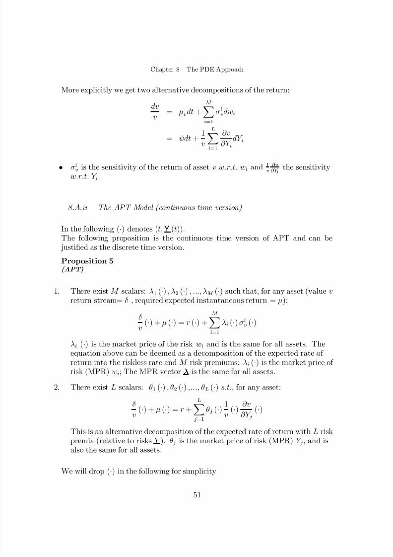
More explicitly we get two alternative decompositions of the return:
dvv
= µvdt +M
Xi=1
σ ivdwi
= ψdt +1v
L
Xi=1
∂ v∂ Y i
dY i
• σ iv is the sensitivity of the return of asset v w.r.t. w i and 1
v∂ v∂ Y i the sensitivity
w.r.t. Y i .
8.A.ii The APT Model (continuous time version)
In the following (·) denotes (t, Y (t)) .The following proposition is the continuous time version of APT and can be justi Þ ed as the discrete time version.
Proposition 5(APT)
1. There exist M scalars: λ 1 (·) , λ 2 (·) , ..., λ M (·) such that, for any asset (value vreturn stream = δ , required expected instantaneous return = µ):
δ v
(·) + µ (·) = r (·) +M
Xi=1
λ i (·) σ iv (·)
λ i (·) is the market price of the risk wi and is the same for all assets. Theequation above can be deemed as a decomposition of the expected rate of return into the riskless rate and M risk premiums: λ i (·) is the market price of risk (MPR) wi ; The MPR vector λ is the same for all assets.
2. There exist L scalars: θ1 (·) , θ2 (·) ,..., θL (·) s.t. , for any asset:δ v
(·) + µ (·) = r +L
X j =1
θ j (·)1v
(·)∂ v∂ Y j
(·)
This is an alternative decomposition of the expected rate of return with L riskpremia (relative to risks Y ). θ j is the market price of risk (MPR) Y j , and isalso the same for all assets.
We will drop (·) in the following for simplicity
51
8/3/2019 Capital Markets and Portfolio Theory, Roland Portait
http://slidepdf.com/reader/full/capital-markets-and-portfolio-theory-roland-portait 58/102
Chapter 8 The PDE Approach
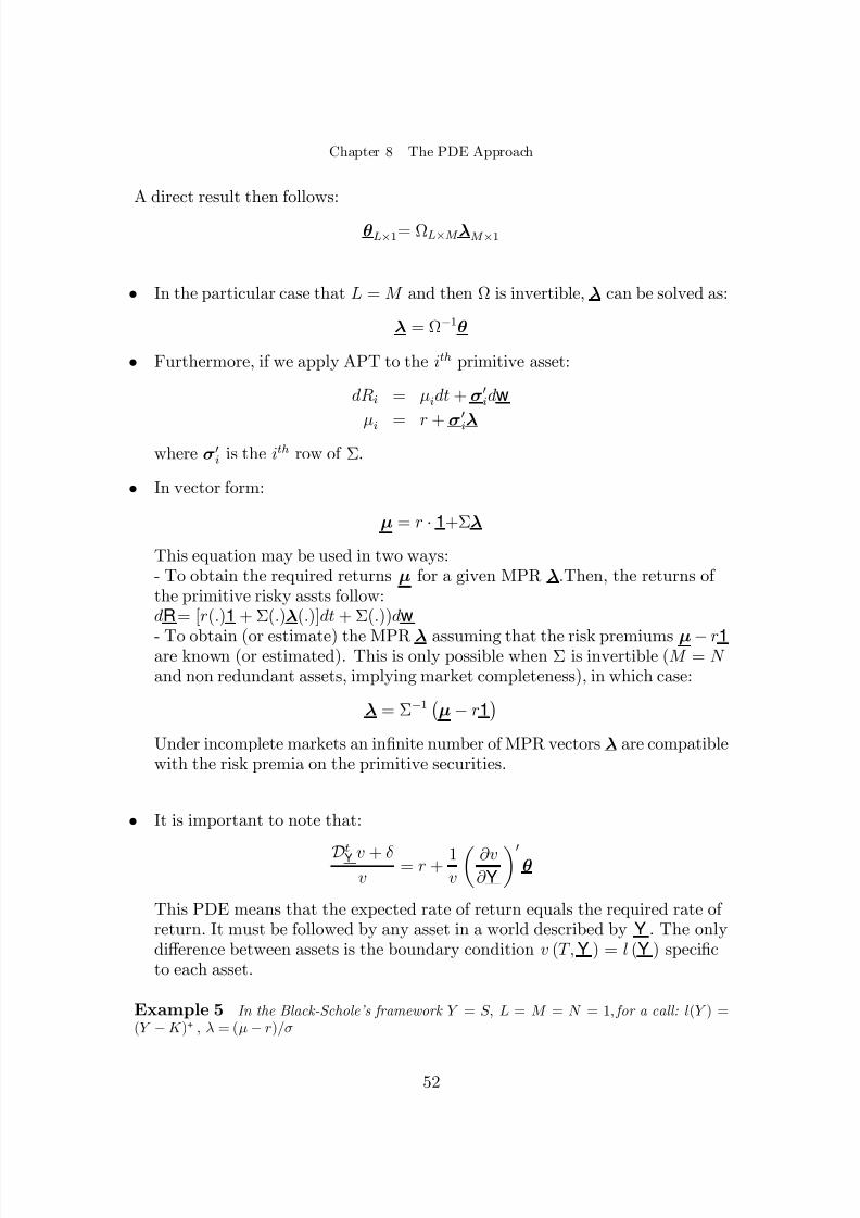
A direct result then follows:
θ L × 1= Ω L × M λ M × 1
• In the particular case that L = M and then Ω is invertible, λ can be solved as:
λ = Ω − 1θ
• Furthermore, if we apply APT to the ith primitive asset:
dR i = µi dt + σ 0i dw
µi = r + σ0i λ
where σ 0i is the ith row of Σ .
• In vector form:
µ = r · 1+ Σ λ
This equation may be used in two ways:- To obtain the required returns µ for a given MPR λ .Then, the returns of the primitive risky assts follow:dR = [r (.)1 + Σ (.)λ (.)]dt + Σ (.))dw
- To obtain (or estimate) the MPR λ assuming that the risk premiums µ −r 1are known (or estimated). This is only possible when Σ is invertible ( M = N and non redundant assets, implying market completeness), in which case:
λ = Σ − 1¡µ −r 1¢Under incomplete markets an in Þ nite number of MPR vectors λ are compatiblewith the risk premia on the primitive securities.
• It is important to note that:
DtY v + δ v
= r + 1vµ∂ v
∂ Y¶0
θ
This PDE means that the expected rate of return equals the required rate of return. It must be followed by any asset in a world described by Y . The onlydiff erence between assets is the boundary condition v (T, Y ) = l (Y ) speciÞ cto each asset.
Example 5 In the Black-Schole’s framework Y = S, L = M = N = 1 , for a call: l(Y ) =(Y −K )+ , λ = ( µ −r )/ σ
52

8/3/2019 Capital Markets and Portfolio Theory, Roland Portait
http://slidepdf.com/reader/full/capital-markets-and-portfolio-theory-roland-portait 59/102
Chapter 8 The PDE Approach
Example 6 A one factor interest rate model with a stochastic risk-free rate r , which is also the state variable. Only bonds are considered and one bond is su ffi cient (the others are redundant), therefore, L = M = N = 1 . We consider such models in the following section.
8.B One Factor Interest Rate Models
• — L = M = 1 , and now Y 1 = r
— dS 0 = S 0 r (t) dt — Let BT (t, r (t)) be the price of a zero coupon bond at t that delivers 1 at T . The
duration of the bond is then T −t
— Several BT may be traded (but they are redundant).
— dr = a [b−r ]dt + σ r (t, r )dw. In Vasicek model σ r (t, r ) = σ constant, and in CIR model σ r = σ√ r
• Write the expected rate of return by applying APT:
Dtr BT
BT = r +
1BT
∂ BT
∂ rθ
This gives:
∂ BT
∂ t+
12
σ2r
∂ 2BT
∂ r 2 + a (b−r )∂ BT
∂ r= rB T +
∂ BT
∂ rθ
with the boundary condition that BT (T ) = 1 ∀T .
• The PDE can be solved in both Vasicek and CIR settings.
8.C Discounting Under Uncertainty
Consider the PDE:
D tY v + δ = rv + µ∂ v
∂ Y¶0
θ ; LC : v(T, Y ) == l(Y )
where LC stands for Limit Conditions. We have:
∂ v∂ t
+ µ∂ v∂ Y¶0
µ Y +12
dY 0 ∂ 2v∂ Y ∂ Y 0dY + δ = rv + µ∂ v
∂ Y¶0
θ
53
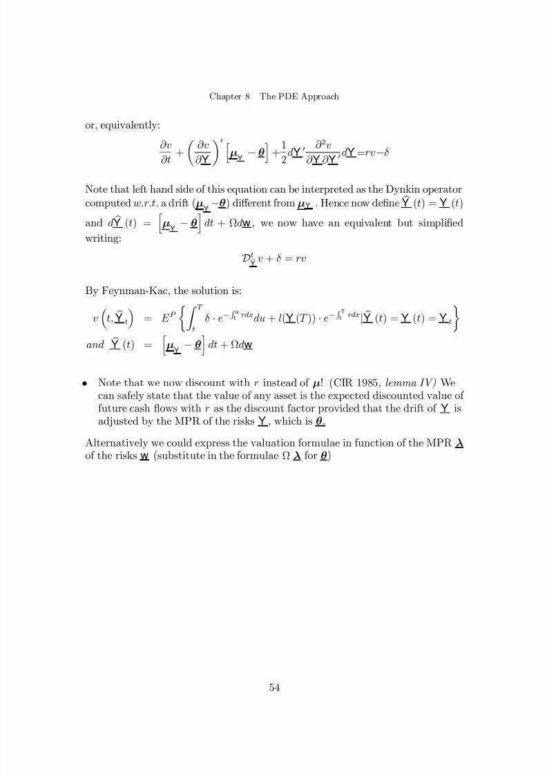
8/3/2019 Capital Markets and Portfolio Theory, Roland Portait
http://slidepdf.com/reader/full/capital-markets-and-portfolio-theory-roland-portait 60/102
Chapter 8 The PDE Approach
or, equivalently:
∂ v∂ t
+ µ∂ v∂ Y¶0hµ Y −θi+
12
dY 0 ∂ 2v∂ Y ∂ Y 0dY = rv−δ
Note that left hand side of this equation can be interpreted as the Dynkin operatorcomputed w.r.t. a drift ( µ Y −θ ) diff erent from µ Y . Hence now de Þ ne bY (t) = Y (t)
and d bY (t) = hµ Y −θidt + Ω dw , we now have an equivalent but simpli Þ edwriting:
D t
bY v + δ = rv
By Feynman-Kac, the solution is:
v³t, bY t´ = E P ½Z T
tδ · e− R u
t rdx du + l(Y (T )) · e− R Tt rdx | bY (t) = Y (t) = Y t¾
and bY (t) = hµ Y −θidt + Ω dw
• Note that we now discount with r instead of µ ! (CIR 1985, lemma IV) Wecan safely state that the value of any asset is the expected discounted value of future cash ß ows with r as the discount factor provided that the drift of Y isadjusted by the MPR of the risks Y , which is θ .
Alternatively we could express the valuation formulae in function of the MPR λof the risks w (substitute in the formulae Ω λ for θ )
54
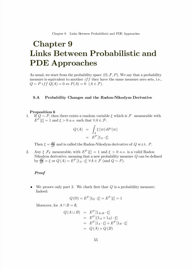
8/3/2019 Capital Markets and Portfolio Theory, Roland Portait
http://slidepdf.com/reader/full/capital-markets-and-portfolio-theory-roland-portait 61/102
Chapter 9 Links Between Probabilistic and PDE Approaches
Chapter 9Links Between Probabilistic andPDE ApproachesAs usual, we start from the probability space (Ω , F , P ). We say that a probabilitymeasure is equivalent to another iff they have the same measure zero sets, i.e.,Q∼P iff Q (A) = 0⇔P (A) = 0 (A∈F ).
9.A Probability Changes and the Radon-Nikodym Derivative
Proposition 61. If Q∼P , then there exists a random variable ξ which is F measurable with
E P [ξ ] = 1 and ξ > 0 a.s. such that ∀A∈F :
Q (A) = Z Aξ ($ ) dP ($ )
= E P [1A · ξ ]
Then ξ = dQdP and is called the Radon-Nikodym derivative of Q w.r.t. P .
2. Any ξ F T measurable, with E P [ξ ] = 1 and ξ > 0 a.s. is a valid RadonNikodym derivative, meaning that a new probability measure Q can be de Þ nedby dQ
dP = ξ or Q (A) = E P [1A · ξ ]∀A∈F (and Q∼P ).
Proof
• We proove only part 2. We check Þ rst that Q is a probability measure;Indeed:
Q (Ω ) = E P [1Ω · ξ ] = E P [ξ ] = 1
Moreover, for A ∩B = ∅,
Q (A∪B ) = E P [1A∪B · ξ ]= E P [(1A + 1 B ) · ξ ]= E P [1A · ξ ] + E P [1B · ξ ]= Q (A) + Q (B )
55
8/3/2019 Capital Markets and Portfolio Theory, Roland Portait
http://slidepdf.com/reader/full/capital-markets-and-portfolio-theory-roland-portait 62/102
Chapter 9 Links Between Probabilistic and PDE Approaches
• We check that Q
∼
P ; Indeed, since ξ > 0 a.s. .,
Q (A) = E P [1A · ξ ] = 0
⇔ P (A) = E P [1A ] = 0
Q.E.D.
• The intuition behind the changing of probability is that, by considering the
probability of an event as a mass, the probability, or the mass, is changed bymultiplying a positive ξ ($ ) (dQ ($ ) = ξ ($ ) dP ($ )) .
• Also, ∀X with E P [X ] < ∞, E Q [X ] = E P [X · ξ ].
9.B Girsanov Theorem
Consider the m-dimensional Brownian Motion w under the probability measureP , the Þ ltration F t (t∈(0, T )) generated by w, and the m-dimensional adaptedprocess λ (·) that satis Þ es integrability conditions ( R t
0 kλ (s)k2 ds deÞ ned,.. ).
Theorem 9(Girsanov Theorem) a) De Þ ne ξ (t) = e− 1
2 R t
0 kλ ( s ) k2 ds − R t
0 λ 0 ( s )d w , then ξ (T ) is a valid Radon-Nikodym derivative:(meaning that: ξ (T ) is F T measurable; E P [ξ ] = 1 ; ξ ≥ 0 a.s. ); Moreover ξ (t) is a P-martingale.b) De Þ ne Q ∼P by dQ
dP = ξ (T ), then ew (t) , w (t) + R t0 λ (s) ds is a standard Q-
Brownian Motion.
9.C Risk Adjusted Drifts: Application of Girsanov Theorem
Consider:
dR = µ dt + Σ N × M dw
We had:
µ = r ·1 + Σ λ
56
8/3/2019 Capital Markets and Portfolio Theory, Roland Portait
http://slidepdf.com/reader/full/capital-markets-and-portfolio-theory-roland-portait 63/102
Chapter 9 Links Between Probabilistic and PDE Approaches
Therefore:
dR = [r ·1 + Σ λ ]dt + Σ dw
We now look for a probability measure Q under which the dynamics of R have adrift of r ·1 (then the asset 0 denominated values S i (t )
S 0 (t ) would be Q-martingales).We know that Q exists and is unique when the market is complete.
Proposition 7Consider the probability Q , equivalent to P , de Þ ned by the Radon-Nikodym deriva-tive:
dQdP
= e− 12 R T
0 kλ ( s )k2 ds − R t
0 λ 0 ( s ) d w
where λ (·) is the market price of risk. Then the instantaneous Q−expected return of any self- Þ nancing asset is r . Moreover, asset 0 denominated values S i ( t )
S 0 ( t ) (as well asthe asset 0 denominated values of self Þ nancing portfolios X ( t )
S 0 ( t ) ) are Q-martingales.Q is thus a risk neutral probability.
Proof
By Girsanov Theorem, ew (t),
w (t) + R t
0 λ (s) ds is a Q-martingale, then:dew (t) , dw (t) + λ (t) dt
⇒ dR = [ r ·1 + Σ λ ]dt + Σ · [dew (t) −λ (t) dt]
⇒ dR = r ·1 ·dt + Σ · dew (t)
We now de Þ ne:
bS (t) ,
S (t)S 0 (t)
with dS 0 (t) = S 0 rdt . Therefore:
d (S/S 0 )S/S 0 = d log
S S 0 +
1
2σ2S dt
=dS S −
dS 0S 0 −
1
2σ2
S dt +1
2σ 2
S dt
=dS S −rdt
If the drift of dS S is r , then the drift of d bS ( t )
bS ( t )will be zero! Thus, by changing the probability
measure from P to Q, the asset 0 denominated values S ( t )S 0 ( t ) are Q-martingales.
Q.E.D.
57

8/3/2019 Capital Markets and Portfolio Theory, Roland Portait
http://slidepdf.com/reader/full/capital-markets-and-portfolio-theory-roland-portait 64/102
Chapter 9 Links Between Probabilistic and PDE Approaches
Remark that when the set of primitive securities is complete ( N = M and Σ
is invertible) only one λ (λ = Σ − 1
¡µ −r 1¢) is compatible with the primitive
returns. Under incomplete markets an in Þ nite number of λ ’s are compatible withthe assumed return dynamics and an in Þ nite number of risk free probabilities canbe constructed.
58
8/3/2019 Capital Markets and Portfolio Theory, Roland Portait
http://slidepdf.com/reader/full/capital-markets-and-portfolio-theory-roland-portait 65/102
8/3/2019 Capital Markets and Portfolio Theory, Roland Portait
http://slidepdf.com/reader/full/capital-markets-and-portfolio-theory-roland-portait 66/102
8/3/2019 Capital Markets and Portfolio Theory, Roland Portait
http://slidepdf.com/reader/full/capital-markets-and-portfolio-theory-roland-portait 67/102
Chapter 11 Numeraire and Probability Changes
Chapter 11Numeraire and ProbabilityChanges
11.A Framework
11.A.i Assets
• Asset returns follow are Ito process following the SDE:
dR = µ dt + Σ dwdS 0 = rS 0dt
dr = µr dt + σ r dw
The coefficients ( µ , Σ , µr , σ r ) are stochastic but satisfy ”Ito” technical conditions
• Assume N ≤M , where N is the number of non-redundant risky assets, andM is the number of Brownian Motions.
11.A.ii Numeraires
De Þ nition 23 A viable numeraire is an admissible self- Þ nancing portfolio with positive val-ues a.s., i.e., (n , N ) is a viable numeraire if:
(n , N ) ∈A0
N (t) > 0 a.s.
Example 7 S 0 (t) = S 0(0)eR t
0 r (u )du
Example 8 BT (t) = price at t of a zero-coupon bond yielding $1 at T
61
8/3/2019 Capital Markets and Portfolio Theory, Roland Portait
http://slidepdf.com/reader/full/capital-markets-and-portfolio-theory-roland-portait 68/102
Chapter 11 Numeraire and Probability Changes
11.B Correspondence Between Numeraires and MartingaleProbabilities
11.B.i Numeraire →Martingale Probabilities
We have studied 0 →P0, now consider any viable numeraire n and the correspon-dence n →Pn .
De Þ nition 24 Pn stands for the set of probabilities equivalent to P yielding n-denominated martingale prices: Pn = nP n ∼P |∀(x , X )∈A0, X ( t )
N ( t ) is a P n martingale oProposition 8For any admissible numeraire (n , N ) and Pn :
1. There is a one-to-one correspondence between P0 (the set of risk-neutralprobabilities) and Pn . Moreover, ∀P 0∈
P0, P 0 →P n is given by:
dP ndP 0 =
N (T )S 0(T ) ·
S 0(0)N (0)
and ∀P n ∈Pn , P n →P 0 is given by:
dP 0dP n
=S 0(T )N (T )
·N (0)S 0(0)
2. Pn 6= ∅⇔AoA ; Pn is a singleton ⇔market is complete
Proof
1. Consider a viable numeraire (n , N ). Without loss of generality assume N (0) =
S (0) = 1 .Let ξ = dP ndP 0
= N (T )S 0 (T ) · S 0 (0)
N (0) . ξ is a viable numeraire; indeed it satis Þ es the threerequirements:(i) ξ is F T -measurable (since N (T ) and S 0(T ) are F T -measurable);(ii) ξ > 0 a.s. (since N (T ) and S 0(T ) are > 0 a.s.);(iii) E P 0 (ξ ) = 1; Indeed, since N (t )
S 0 (t ) is a P 0 martingale: E P 0 ( N (T )S 0 (T ) ) = N (0)
S 0 (0) . There-
fore E P 0 (ξ ) = E P 0 ³N (T )S 0 (T ) · S 0 (0)
N (0) ´= 1 .Then ξ deÞ nes uniquely a probability P n ∼ P 0. Moeover such P n belongs to Pn ;indeed, for any (x , X ) in A
0
:
62

8/3/2019 Capital Markets and Portfolio Theory, Roland Portait
http://slidepdf.com/reader/full/capital-markets-and-portfolio-theory-roland-portait 69/102
Chapter 11 Numeraire and Probability Changes
E P n ( X (T )N (T ) ) = E P 0 ( X (T )
N (T ) ξ ) = E P 0 ( X (T )N (T )
N (T )S 0 (T )
S 0 (0)N (0) ) = E P 0 ( X (T )
S 0 (T ) ) S 0 (0)N (0) = X (0)
S 0 (0)S 0 (0)N (0) =
X (0)N (0) , hence X
N is a P N -martingale. An analogous argument shows that 1/ ξ = dP 0
dP ndeÞ nes the correspondance between Pn and P0 and the two sets are thus in a oneto one relation through this procedure.2. Follows from 1. and from the fact that 2. is true for P0
Q.E.D.
More generally, given any (n , N ) and (n 0, N 0)∈N , there is a one-to-one corre-spondence between Pn and Pn 0 deÞ ned by:
dP n 0
dP n= N 0(T )
N (T )· N (0)
N 0(0)
with the possible assumption that N (0) = N 0(0) = 1
11.B.ii Probability →Numeraire
Let us state the following without proof
Proposition 9For any probability Q∼to P there exists a numeraire nQ such that the nQ −denominated values of all admissible and self- Þ nanced assets or portfolios are Q-martingales.This numeraire is unique (up to a scale factor). The uniqueness of this martin-gale numeraire prevails even in incomplete markets and when asset prices follow semi-martingales
11.C Summary
• In AoA: — There exists a set P0 of probabilities equivalent to P (the true or historical probability)
such that ∀P 0∈P0 and ∀(x ,X )∈A0 (the set of admissible and self- Þ nancing strategies),
the S 0(t) denominated price X ( t )S 0 ( t ) is a P 0 -martingale.
— P0 is a singleton when the market is complete.
— De Þ ne N as the set of all admissible numeraires. Then N ∈ N iff (n ,N )∈A0 and N (t) > 0 a.s. .
— ∀(n ,N )∈N there exists Pn ∼P such that ∀P n ∈
Pn and ∀(x ,X )∈A0, the N (t)denominated price X ( t )
N ( t ) is a P n -martingale.
63
8/3/2019 Capital Markets and Portfolio Theory, Roland Portait
http://slidepdf.com/reader/full/capital-markets-and-portfolio-theory-roland-portait 70/102
Chapter 11 Numeraire and Probability Changes
— In the general case, given any (n , N ) and (n 0, N 0)
∈
N , there is a one-to-one correspondence between Pn and Pn 0 de Þ ned by:
dP n 0
dP n=
N 0(T )N (T )
·N (0)N 0(0)
with the possible assumption that N (0) = N 0(0) = 1
— Conversely, ∀Q∼P , there exists a unique numeraire N Q such that the N Q denominated prices are Q-martingales.
• Then why not consider a portfolio (h ,H ) that yields martingale prices underthe true probability P ? This question is addressed in the following section.
64
8/3/2019 Capital Markets and Portfolio Theory, Roland Portait
http://slidepdf.com/reader/full/capital-markets-and-portfolio-theory-roland-portait 71/102
Chapter 12 The Numeraire (Growth Optimal) Portfolio
Chapter 12The Numeraire (Growth Optimal)Portfolio
12.A De Þ nition and Characterization
12.A.i De Þ nition of the Numeraire (h , H )
De Þ nition 25 The numeraire portfolio is the unique portfolio (h , H )∈ N such that ∀(x , X )∈A0, X ( t )
H ( t ) is a P -martingale, i.e.:
E t ·X (T )H (T )¸=
X (t)H (t)
where E t [·] = E [·|F t ] is the conditional expectation computed with the true probability.
The price of the asset is then given as:
X (t) = H (t) · E t ·X (T )H (T )¸
with H (t )H (T ) often being referred to as the “discount factor” or the “pricing kernel”.
(h , H ) is also called the “growth optimal portfolio” (Merton), the “log-optimalportfolio”, and the “numeraire portfolio” (Long).
12.A.ii Characterization and Composition of (h , H )
Theorem 101. (h , H ) is the strategy that maximizes the expected log of the terminal wealth
W (T ), i.e. it solves the program:
max(x ,X )∈A 0
E 0 [logX (T )]
65
8/3/2019 Capital Markets and Portfolio Theory, Roland Portait
http://slidepdf.com/reader/full/capital-markets-and-portfolio-theory-roland-portait 72/102
8/3/2019 Capital Markets and Portfolio Theory, Roland Portait
http://slidepdf.com/reader/full/capital-markets-and-portfolio-theory-roland-portait 73/102
Chapter 12 The Numeraire (Growth Optimal) Portfolio
Maximizing E [R0,T 0 ] then implies a two-step maximization procedure:max E [R0,T ] and max E [RT,T 0 ].
Q.E.D.
The previous results are also valid for semi-martingale prices, but in the following,it is assumed that prices and rates of return follow Ito process, i.e.
dR = µ dt + Σ dwdr = µr dt + σ r dw
with R an N × 1 vector, Σ an N × M matrix with rank N (there is no redundantasset, so N ≤M ), and the coe fficients obey the usual technical conditions so thatthere exists a solution for the SDE.
Theorem 11The composition of h is:
h = Γ − 1£µ −r ·1¤with Γ = ΣΣ 0 being an invertible N × N matrix.
Proof
Because the Log utility is myopic, optimizing over ( t,T ) implies optimizing over [t, t + dt] ;In [t, t + dt]
maxx
E t [logX (t + dt)]
⇔ maxx
E t [logX (t + dt) −log X (t)]
⇔ maxx
E t [d log X ]
By Ito’s lemma, d log X = dXX − 1
2
¡dXX
¢2. It is also known that:
dX X
= ( 1 −x 0 · 1) rdt + x 0Σ dw
= ©r + x 0£µ −r ·1¤ªdt + x 0Σ dw
Therefore, the maximization program is now:
maxx
E t [d log X ]⇔maxx ©r + x 0£µ −r ·1¤ªdt −
1
2x0Σ dw dw 0Σ 0x
With dw dw 0 = I · dt
maxx
E t [d log X ]⇔maxx ½r + x 0£µ −r ·1¤− 1
2x 0Γ x¾dt
67
8/3/2019 Capital Markets and Portfolio Theory, Roland Portait
http://slidepdf.com/reader/full/capital-markets-and-portfolio-theory-roland-portait 74/102
Chapter 12 The Numeraire (Growth Optimal) Portfolio
Leave out dt and apply the Þ rst order condition gives:
£µ −r ·1¤−Γ h = 0⇔h = Γ − 1£µ −r ·1¤Q.E.D.
Corollary 5 (h ,H ) is instantaneously mean-variance e ffi cient, hence homothetical (propor-tional) to the tangent portfolio (m ,M ), i.e.
h =1
ktm
= £10 · Γ − 1¡µ −r ·1¢¤m
with
kt =1
10 · Γ − 1 ¡µ −r ·1¢and
m = kt Γ − 1
¡µ
−r ·1
¢(the weights in m sum up to one while in h they don’t; h is a combination of m and asset 0).We have not excluded the possibility that N < M . But now assume that N = M ; then:
Corollary 6 When the market is complete and Σ N × N is invertible, the market price of risk can be derived as a function of the risk premia 6 :
λ = Σ − 1¡µ −r ·1¢The composition of the numeraire portfolio can now be expressed in terms of λ as:
h =Γ − 1
£µ −r ·1¤= Σ 0− 1 Σ − 1£µ −r ·1¤= Σ 0− 1 λ
6 When the market is not complete, λ cannot be explicitly speci Þ ed. For the i t h asset, for instance,
µ i− r =
M
X j = 1
σ i j λ j
With N < M , the system of N equations does not yield an unique solution for λ 1 ,..., λ M
68
8/3/2019 Capital Markets and Portfolio Theory, Roland Portait
http://slidepdf.com/reader/full/capital-markets-and-portfolio-theory-roland-portait 75/102
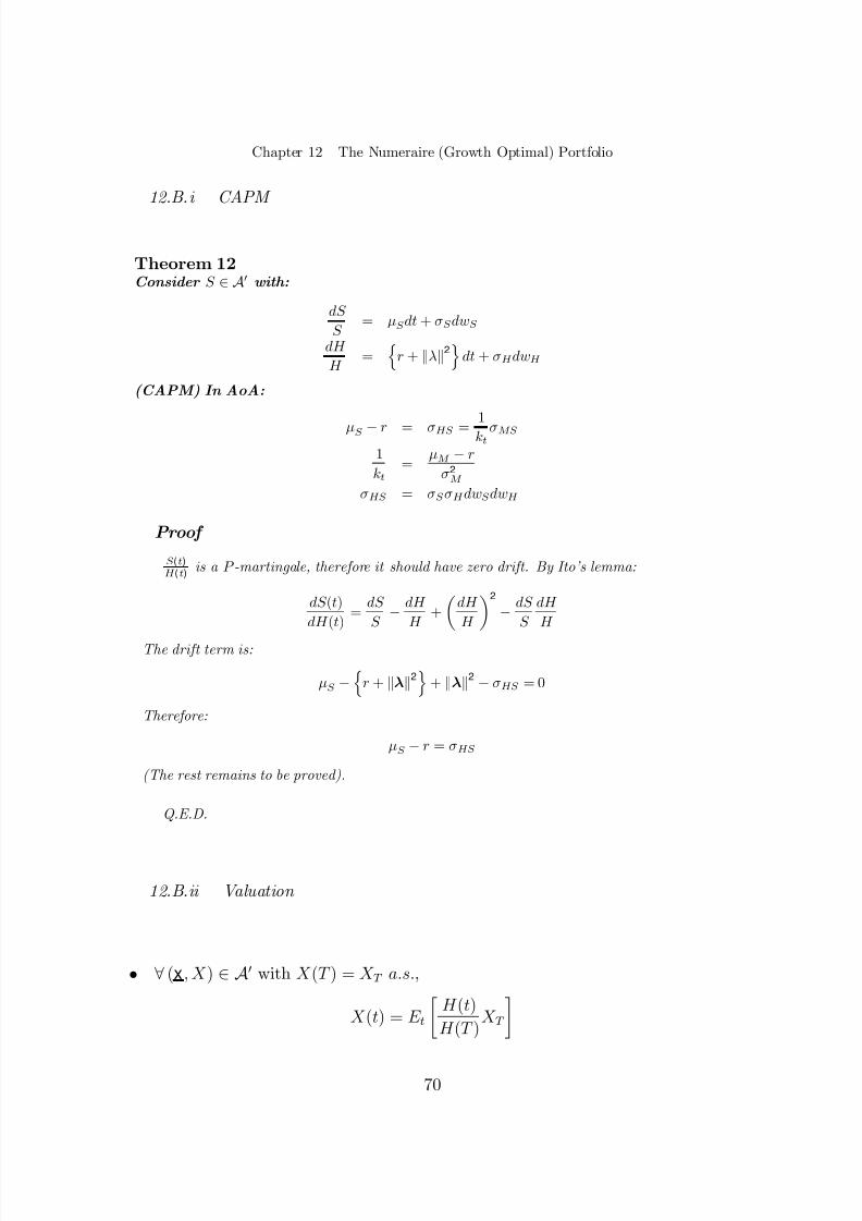
8/3/2019 Capital Markets and Portfolio Theory, Roland Portait
http://slidepdf.com/reader/full/capital-markets-and-portfolio-theory-roland-portait 76/102
Chapter 12 The Numeraire (Growth Optimal) Portfolio
12.B.i CAPM
Theorem 12Consider S ∈A0 with:
dS S
= µS dt + σS dwS
dH H
= nr + kλ k2odt + σ H dwH
(CAPM) In AoA:
µS −r = σHS =1
kt σ MS
1
kt=
µM −rσ 2
M
σ HS = σS σH dwS dwH
Proof S ( t )H ( t ) is a P -martingale, therefore it should have zero drift. By Ito’s lemma:
dS (t)dH (t)
=dS S −
dH H
+ µdH H ¶2
−dS S
dH H
The drift term is:
µS −nr + kλ k2o+ kλ k2
−σHS = 0
Therefore:
µS −r = σ HS
(The rest remains to be proved).
Q.E.D.
12.B.ii Valuation
• ∀(x , X )∈A0 with X (T ) = X T a.s. ,
X (t) = E t ·H (t)H (T )
X T ¸70
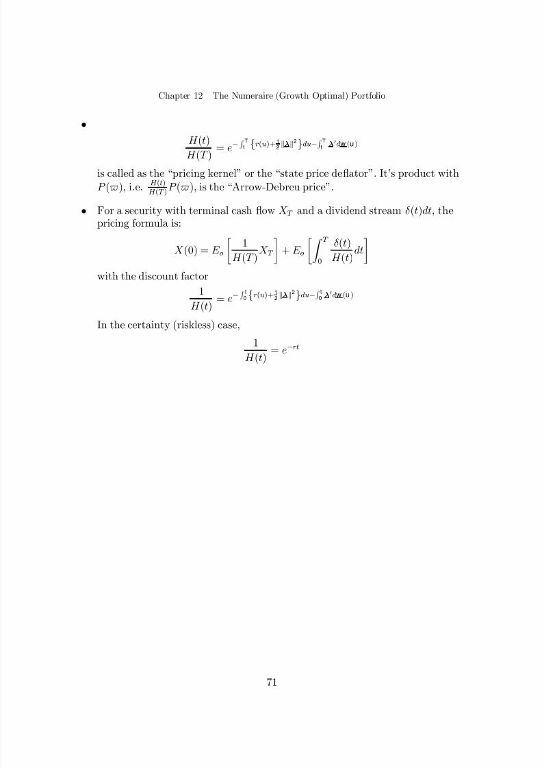
8/3/2019 Capital Markets and Portfolio Theory, Roland Portait
http://slidepdf.com/reader/full/capital-markets-and-portfolio-theory-roland-portait 77/102
Chapter 12 The Numeraire (Growth Optimal) Portfolio
•H (t)H (T )
= e− R Tt r (u )+ 1
2 kλ k2 du − R Tt λ 0 dw (u )
is called as the “pricing kernel” or the “state price de ß ator”. It’s product withP ($ ), i.e. H (t )
H (T ) P ($ ), is the “Arrow-Debreu price”.
• For a security with terminal cash ß ow X T and a dividend stream δ (t)dt, thepricing formula is:
X (0) = E o
·1
H (T )X T
¸+ E o
·Z T
0
δ (t)H (t)
dt
¸with the discount factor1
H (t)= e− R t
0 r (u )+ 12 kλ k2 du − R t
0 λ 0 dw (u )
In the certainty (riskless) case,
1H (t)
= e− rt
71
8/3/2019 Capital Markets and Portfolio Theory, Roland Portait
http://slidepdf.com/reader/full/capital-markets-and-portfolio-theory-roland-portait 78/102
8/3/2019 Capital Markets and Portfolio Theory, Roland Portait
http://slidepdf.com/reader/full/capital-markets-and-portfolio-theory-roland-portait 79/102
Chapter 13 Dynamic Consumption and Portfolio Choices (The Merton Model)
Chapter 13Dynamic Consumption andPortfolio Choices (The MertonModel)
13.A Framework
13.A.i The Capital Market
We consider a di ff usion-state variables model.
Let L be the number of state variables and Y be the vector describing the statesof the economy, with
dY L × 1 = µ Y (t, Y (t )) · dt + Ω L × M (t, Y (t )) · dw M × 1
• There are N + 1 assets in the economy. The returns of the N risky assetsfollow the diff usion process:
dR N × 1 = µ (t, Y (t )) · dt + Σ N × M (t, Y (t )) · dw M × 1
73
8/3/2019 Capital Markets and Portfolio Theory, Roland Portait
http://slidepdf.com/reader/full/capital-markets-and-portfolio-theory-roland-portait 80/102
Chapter 13 Dynamic Consumption and Portfolio Choices (The Merton Model)
and the riskless return follows:
dr = µr (t, Y (t )) · dt + σ 0r (t, Y (t )) · dw
S 0(t) = eR t0 r (u )du
• The usual technical (integrability) conditions and a frictionless andcontinuously open market are assumed.
13.A.ii The Investors (Consumers)’ Problem
For an investor with wealth X (t) at time t, the Budget Constraint in [t, t + dt] is:
dX = X (t)©r (t) + x0(t )£µ (t )−r (t) · 1¤dt + x 0(t )Σ dwª−c(t)dt + y(t)dt
where the Þ rst term in the right hand side of the equation is the gain of theportfolio, the second term Consumption , and the third term Income .
• The optimization program, denoted by M , is:
(M
) maxc,xE
t
½Z T
tU
(c
(u
), u
)du
+B
(X
(T
))¾s.t. the Budget Constraint
where U (·) and B (·) are both utility functions ( B (·) may be interpreted asthe utility of a bequest). They are state independent but they do depend ont. Additional restrictions imposed on U (·) and B (·) are:
— U (·) and B (·) are strictly concave.
— U 0(0) and B 0(0) = ∞ ; U (0) and B (0) = −∞so as to preclude negative consumption or bequest.
13.B The Solution
13.B.i Sketch of the Method
74
8/3/2019 Capital Markets and Portfolio Theory, Roland Portait
http://slidepdf.com/reader/full/capital-markets-and-portfolio-theory-roland-portait 81/102
8/3/2019 Capital Markets and Portfolio Theory, Roland Portait
http://slidepdf.com/reader/full/capital-markets-and-portfolio-theory-roland-portait 82/102
Chapter 13 Dynamic Consumption and Portfolio Choices (The Merton Model)
where:
µX = X £r (·) + x 0¡µ (·) −r (·) 1¢¤−c (t)
σ2X = X 2x 0Γ x
Γ = ΣΣ 0
dY dY 0 = ΩΩ 0dt, with ΩΩ 0 = V or:
dY i dY j = V ij dt
dXdY i = X (x 0Σ dw ) Ω 0idw
= X x 0ΣΩ idt
where Ω 0i is the ith row of Ω .
The problem is now:
maxc, x
U (c, t) + Dc, x
X, Y (J )
or equivalently (c∗ (t) , x∗ (t)) solve:
maxc,x ψ (t,c, x ; X (t) , Y (t))
Recall that the maximum of ψ(·) is zero; We obtain thus two equations (Bellmanconditions):
maxc, x
ψ (t,c, x ; X (t) , Y (t))(1)= ψ (t, c∗ (t) , x∗ (t) ; X (t) , Y (t))
(2)= 0
• (a) The Þ rst equation implies the Þ rst order conditions:
∂ψ∂ c
(t, c∗ (t) , x∗ (t) ; X (t) , Y (t)) = 0
and∂ψ∂ x
(t, c∗ (t) , x∗ (t) ; X (t) , Y (t)) = 0
(b) The second equation implies that the PDE governing J is:
U (c∗, t) + ³Dc∗ ,x ∗
X, Y (J )´= 0
76
8/3/2019 Capital Markets and Portfolio Theory, Roland Portait
http://slidepdf.com/reader/full/capital-markets-and-portfolio-theory-roland-portait 83/102
Chapter 13 Dynamic Consumption and Portfolio Choices (The Merton Model)
with limit condition:
J (T,X, Y ) = B (X )
The PDE governing J (theoretically) determines J , which in turn allows the com-putation of ψ (via Dc, x
Y (J ) computed previously). Then the Þ rst order conditionswill determine the optimal (c∗ (t) , x∗ (t)) . This methodology yields only in somefew cases a closed form solution for the optimal portfolio x∗, but it allows to provethat it has the general form presented in the following paragraphs.
13.B.ii Optimal portfolios and L + 2 funds separation
Proposition 10The optimal portfolio as a solution of program M writes:
x∗ (·) = A (·) h +L
Xk = 1
Ak (·) h k (·)
where
• A (·) is the relative Risk Tolerance de Þ ned as:
A ≡ −1X
·J X
J XX
• Ak depends on the indirect utility function and is its sensitivity w.r.t. dY k
• h is the (instantaneously mean-variance e fficient, ...) log optimal portfoliostudied in a previous chapter:
h = Γ − 1
¡µ −r1
¢• h k (k = 1 , 2,...,L ) are hedge portfolios with a return perfectly correlated withdY k ; they are aimed to hedge against unfavorable shifts of the investmentopportunity set induced by movements of Y k .
Proof
Follows from the Bellman conditions (1 ) and (2) (see Merton)
Q.E.D.
77
8/3/2019 Capital Markets and Portfolio Theory, Roland Portait
http://slidepdf.com/reader/full/capital-markets-and-portfolio-theory-roland-portait 84/102
8/3/2019 Capital Markets and Portfolio Theory, Roland Portait
http://slidepdf.com/reader/full/capital-markets-and-portfolio-theory-roland-portait 85/102
Chapter 13 Dynamic Consumption and Portfolio Choices (The Merton Model)
Consider now the general case with L state variables (and thus L + 2 fund sepa-ration). The generalized CAPM writes:
µS −r = β mS (µm −r ) +L
Xk =1
β kS ( bµk −r )
where bµk is the expected rate of return of the hedge portfolio h k , and
β kS =cov (dRS , dR k )
var (dRk )
79
8/3/2019 Capital Markets and Portfolio Theory, Roland Portait
http://slidepdf.com/reader/full/capital-markets-and-portfolio-theory-roland-portait 86/102
Chapter 14 THE ”EQUIVALENT” STATIC PROBLEM (Cox-Huang, Karatzas approach)
Chapter 14THE ”EQUIVALENT”STATIC PROBLEM (Cox-Huang,Karatzas approach)
14.A Transforming the dynamic into a static problem
We will assume in the following that:
• The market is AoA
• S follows a multivariate Ito process: dR= µ (·)dt + Σ (·)dw
14.A.i The pure portfolio problem
In this section the market may be incompleteLet us specialize the Merton problem into a pure portfolio decision:
maxx
E [U (X T )]
s.t. ½dX X = £r (·) + x 0¡µ −r 1¢¤dt + x0Σ dw
X (0) = X 0
where U (X T ) = B (X T ) is the concave bequest function, and the Þ rst constraintis the self-Þ nancing condition. The solution of M is (x∗, X ∗), with X ∗ (T )
≡X ∗T .
Also consider program P involving two optimization steps (P 1) and (P 2):
(P 1) : maxX T ∈L 2
E [U (X T )]
s.t. ( X T ∈C a
E hX TH T | F 0i= X 0
and
(P 2) : Find (x∗∗, X ∗∗) attaining X ∗∗T
80
8/3/2019 Capital Markets and Portfolio Theory, Roland Portait
http://slidepdf.com/reader/full/capital-markets-and-portfolio-theory-roland-portait 87/102
Chapter 14 THE ”EQUIVALENT” STATIC PROBLEM (Cox-Huang, Karatzas approach)
The solution to (P 1) is the random contingent claim X ∗∗T . But since X ∗∗T
∈
C a
(i.e. the set of attainable contingent claims), it is attainable through at least onestrategy (x∗∗, X ∗∗)∈A0 with X ∗∗(0) = X 0.
Proposition 111. The solution X ∗ (T ) obtained through (M ) solves (P 1)
2. The solution (x∗∗, X ∗∗) obtained through (P ) solves (M )
3. Under ’mild’ technical conditions (e.g., U (·) strictly concave), X ∗T = X ∗∗T a.s..
Proof
1. X ∗T meets the constraints of (P 1). Indeed,
— X ∗T ∈C a since it is attainable through x∗
— X ∗ (t) being the value process of a self- Þ nancing strategy, X ∗ ( t )H ( t ) is a P -martingale,
i.e.
E ·X ∗ (T )H (T )
| F 0¸= X (0) = X 0
Hence X ∗
(T ) meets the constraints of (P 1 ). but, since X ∗∗
(T ) is the solution of (P 1):
E [U (X ∗∗ (T ))] ≥E [U (X ∗ (T ))]
2. On the other hand, (x∗∗, X ∗∗) is self-Þ nancing and feasible (therebysatisfying the constraints of M ) and (x∗, X ∗) solves M , so:
E [U (X ∗∗(T ))] ≤E [U (X ∗ (T ))]
We can conclude from the two last inequalities that:
E [U (X ∗∗(T ))] = E [U (X ∗ (T ))]
Thus X ∗ (T ) solves (P 1) and (x∗∗, X ∗∗) solves (M )
3. (proof by contradiction ) Suppose X ∗T and X ∗∗T are not equal a.s. . Thenthere exists a subset D of Ω with strictly positive measure where ∀$ ∈D
X ∗T (ω) 6= X ∗∗T (ω)
Consider
bX T ≡
X ∗T + X ∗∗T
2
81

8/3/2019 Capital Markets and Portfolio Theory, Roland Portait
http://slidepdf.com/reader/full/capital-markets-and-portfolio-theory-roland-portait 88/102
Chapter 14 THE ”EQUIVALENT” STATIC PROBLEM (Cox-Huang, Karatzas approach)
bX T is attainable by a buy-and-hold strategy with initial weight 1
2 in (x∗, X ∗)and 1
2 in (x∗∗, X ∗∗). Because of the strict concavity of U (·),∀$ ∈D:
U ³bX T ´≡ U µX ∗T + X ∗∗T
2 ¶>
U (X ∗T ) + U (X ∗∗T )2
Since ∀$ ∈Ω −D, X ∗T (ω) = X ∗∗T (ω):
E
hU
³bX T
´i>
E [U (X ∗T )] + E [U (X ∗∗T )]2
= E [U (X ∗T )] = E [U (X ∗∗T )]
That is to say that there exists a feasible and attainable strategy which yieldsa higher expected utility than either X ∗T or X ∗∗T . This is in contradictionwith our maximization programs M and (P 1).
Q.E.D.
The static program (P 1) can be interpreted as a static choice of a contingentclaim, or a self-Þ nancing strategy, out of an in Þ nite number of them with a staticbudget constraint E
hX ∗ (T )H (T ) | F 0
i= X 0
14.A.ii The consumption-portfolio problem
• The dynamic program M writes:
M : maxx , c
E ·Z T
0U (c (t) , t ) dt + U (X T )¸
s.t. ½dX = X £¡r + x0
¡µ −r1¢dt¢+ x
0Σdw¤−c (t) dtX (0) = X 0
• The static program P writes:
—
(P 1) : maxX T ,c
E "Z T
0U (c (t) , t ) dt + U (X T )#
s.t. : E 0"Z T
0
c (t)H (t)
dt +X T
H (T )#= X 0
82
8/3/2019 Capital Markets and Portfolio Theory, Roland Portait
http://slidepdf.com/reader/full/capital-markets-and-portfolio-theory-roland-portait 89/102
8/3/2019 Capital Markets and Portfolio Theory, Roland Portait
http://slidepdf.com/reader/full/capital-markets-and-portfolio-theory-roland-portait 90/102
Chapter 14 THE ”EQUIVALENT” STATIC PROBLEM (Cox-Huang, Karatzas approach)
• We prove the theorem is a discrete (countable) state space Ω . Ouroptimization program is now:
(P 01) : max
X T ($ ) X$ ∈Ω
p ($ ) U (X T ($ ))
s.t. : X$ ∈Ω
p ($ )X T ($ )H T ($ )
= X 0
The Lagrangian writes:
L (X T , θ) =
X$∈Ω
p($ ) U (X T ($ )) −θ
X$∈Ω
p ($ )X T ($ )H T ($ )
By Þ rst order condition, for all $ in Ω :
p ($ ) U 0(X ∗∗T ($ )) −θp ($ )
H T ($ )= 0
hence, for all $ :
X ∗∗T ($ ) = U 0− 1µθH T ($ )
where θ is such that the budget constraint is satis Þ ed:
E 0·1H T
U 0− 1µθH T ¶¸= X 0
• The more general proof for continuous measurable state space Ω involvescalculus of variations (Euler Theorem).
Q.E.D.
Remark 16 The optimal terminal wealth X ∗∗T is the solution to (P 1 ). The optimal portfoliostrategy x∗∗ as solution to (P 2 ) remains to be found. This is, however, a di ffi cult task.
Remark 17 X ∗∗T may be negative, although for some utility functions, such as CRRA,X ∗∗T > 0 a.s. . In general, to make the problem ’more realistic’, an additional constraint such as X ∗∗T > K a.s. may be involved. It can be shown that in this case the solution is X ∗∗T , attainable with an initial wealth = X 0 −P without constraint, plus a put on X ∗∗T with strike K ( P is the price of this put).
84

8/3/2019 Capital Markets and Portfolio Theory, Roland Portait
http://slidepdf.com/reader/full/capital-markets-and-portfolio-theory-roland-portait 91/102
8/3/2019 Capital Markets and Portfolio Theory, Roland Portait
http://slidepdf.com/reader/full/capital-markets-and-portfolio-theory-roland-portait 92/102
Chapter 14 THE ”EQUIVALENT” STATIC PROBLEM (Cox-Huang, Karatzas approach)
Example 11 Quadratic utility:
U (X ) = X −1
2q X 2
where q is the risk tolerance. The solution writes:
X ∗∗T = q −θ
H T
So the optimal portfolio would consist of a long position in q units of zero coupon bond and a short position in 1
H ( t ) .
14.B.iii Solution of the consumption-portfolio problem
The static program (P 1) writes:
(P 1) : maxX T ,c
E ·Z T
0U (c (t) , t) dt + U (X T )¸
s.t. : E 0·Z T
0
c (t)H (t)
dt +X T
H (T )¸= X 0
Consider a discrete (countable) state space Ω . The Lagrangian writes:
L (X T , c (t) , θ) = X$ ∈Ω
p ($ )·Z T
0U (c (t, $ )) dt + U (X T ($ ))¸
−θX$ ∈Ω
p($ )·Z T
0
c (t, $ )H (t, $ )
dt +X T ($ )H T ($ )¸
By Þ rst order condition:
∂ L∂ c ($, t ) = p ($ )·U 0(c∗∗(t)) − θH (t)¸= 0
and∂ L
∂ X T ($ )= p ($ )·U 0(X ∗∗T ($ )) −
θH T ($ )¸= 0
Thus:
U 0(c∗∗(t)) =θ
H (t)
86
8/3/2019 Capital Markets and Portfolio Theory, Roland Portait
http://slidepdf.com/reader/full/capital-markets-and-portfolio-theory-roland-portait 93/102
Chapter 14 THE ”EQUIVALENT” STATIC PROBLEM (Cox-Huang, Karatzas approach)
and
U 0(X ∗∗T ) −θ
H T
Note that since H (0) = 1 ,
U 0(c∗∗(0)) = θ
14.B.iv General method for obtaining the optimal strategy x∗∗
Consider the case of state variable model where the state is described by Y (t):
dY (t) = µ Y (t ) (·) dt + Ω dw
• The method can be sketched as follows:
(a) By martingale property:
X ∗∗(t) = H (t) E µX ∗∗
T H (T ) | Y t
¶≡Ψ (t, Y t )
The difficulty comes from the computation of Ψ (t, Y t ). Apply Ito’s lemma:
dX ∗∗
X ∗∗=
dΨ
Ψ
= [·]dt +1Ψ µ∂ Ψ
∂ Y¶0Ω dw
(b) Note also that (x∗∗, X ∗∗) is a portfolio strategy, so:
dX ∗∗
X ∗∗ = [·]dt + x∗∗
0Σ dw
(c) Therefore, by identi Þ cation:
x∗∗0Σ =1Ψ µ∂ Ψ
∂ Y¶0Ω
When M = N and Σ is invertible:
x∗∗0 =1Ψ µ∂ Ψ
∂ Y¶0ΩΣ − 1
87
8/3/2019 Capital Markets and Portfolio Theory, Roland Portait
http://slidepdf.com/reader/full/capital-markets-and-portfolio-theory-roland-portait 94/102

8/3/2019 Capital Markets and Portfolio Theory, Roland Portait
http://slidepdf.com/reader/full/capital-markets-and-portfolio-theory-roland-portait 95/102
Chapter 14 THE ”EQUIVALENT” STATIC PROBLEM (Cox-Huang, Karatzas approach)
Remark 19
h−c∗∗ U 00 (c ∗∗ )
U 0 (c ∗∗ )
iis the relative risk aversion of the representative agent.
89

8/3/2019 Capital Markets and Portfolio Theory, Roland Portait
http://slidepdf.com/reader/full/capital-markets-and-portfolio-theory-roland-portait 96/102
PART VISTRATEGIC ASSET
ALLOCATION

8/3/2019 Capital Markets and Portfolio Theory, Roland Portait
http://slidepdf.com/reader/full/capital-markets-and-portfolio-theory-roland-portait 97/102
Chapter 15 The problems
Chapter 15The problems
91
8/3/2019 Capital Markets and Portfolio Theory, Roland Portait
http://slidepdf.com/reader/full/capital-markets-and-portfolio-theory-roland-portait 98/102
Chapter 16 The optimal terminal wealth in the CRRA, mean-variance and HARA cases
Chapter 16The optimal terminal wealth inthe CRRA, mean-variance andHARA cases
16.A Optimal wealth and strong 2 fund separation
16.B The minimum norm return
92
8/3/2019 Capital Markets and Portfolio Theory, Roland Portait
http://slidepdf.com/reader/full/capital-markets-and-portfolio-theory-roland-portait 99/102
Chapter 17 Optimal dynamic strategies for HARA utilities in two cases
Chapter 17Optimal dynamic strategies forHARA utilities in two cases
17.A The GBM case
17.B Vasicek stochastic rates with stock trading
93
8/3/2019 Capital Markets and Portfolio Theory, Roland Portait
http://slidepdf.com/reader/full/capital-markets-and-portfolio-theory-roland-portait 100/102
Chapter 18 Assessing the theoretical grounds of the popular advice
Chapter 18Assessing the theoretical groundsof the popular advice
18.A The bond/stock allocation puzzle
18.B The conventional wisdom
94
8/3/2019 Capital Markets and Portfolio Theory, Roland Portait
http://slidepdf.com/reader/full/capital-markets-and-portfolio-theory-roland-portait 101/102
Chapter 18 Assessing the theoretical grounds of the popular advice
ReferencesARTICLES
• BAJEUX I. , R. PORTAIT, 1992, Méthodes probabilistes d’évaluation etmodèles à variables d’état: une synthèse, Finance
• BAJEUX I, R. PORTAIT, 1997, The numeraire portfolio : A new perspectiveon Þ nancial theory, European Journal of Finance December
• BAJEUX I., R. PORTAIT, 1998, Dynamic asset allocation in a mean-varianceframework, Management Science November
• BAJEUX I. JORDAN J. and R. PORTAIT, 1999, Dynamic asset allocationfor stocks, bonds and cash
• BAJEUX I. JORDAN J. and R. PORTAIT, 2000, An asset allocation puzzle :comment. Forthcoming, American Economic Review
• CANNER N., N.G. MANKIW AND D.N. WEIL, 1997, An asset allocationpuzzle, American Economic Review.
• COX J. and C.F. HUANG, 1989, Optimal consumption and Portfolio policieswhen asset prices follow a di ff usion process, Journal of economic Theory , 49.
• COX J., J, INGERSOL and S.ROSS., 1985, An intertemporal generalequilibrium model of asset prices, Econometrica ,53
• DYBVIG P. and C.F. HUANG, 1989, Nonnegative wealth, AOA and feasibleconsumption plans, Review of Financial studies vol 1, number 4
• GEMAN H., EL KAROUI N. and ROCHET J.C, 1995, Changes of numerairearbitrage and option prices, Journal of Applied Probabilities, 2
• HANSEN L.P. and RICHARD S., 1987, the role of conditioning informationin deducing testable restrictions implied by dynamic asset pricing models,Econometrica, vol 55, N 3, 587-613.
• HARRISON J.M. and K. KREPS, 1979, Martingales and arbitrage inmultiperiod security markets, Journal of Economic Theory, 20.
• HARRISON J.M. and S. PLISKA, 1981, Martingales and the Stochasticintegrals in the theory of continuous trading, Stochastic processes and theirapplications ,11
95
8/3/2019 Capital Markets and Portfolio Theory, Roland Portait
http://slidepdf.com/reader/full/capital-markets-and-portfolio-theory-roland-portait 102/102
Chapter 18 Assessing the theoretical grounds of the popular advice
• HE H. and PEARSON N.D., 1991, consumption and portfolio policies withincomplete markets and short sale constraints, Journal of Economic Theory,54, 259-305.
• KARATZAS, I., J. LEHOCZKY and S. SCHREVE, 1987, Optimal Portfolioand Consumption Decisions for a “Small Investor“ on a Finite Horizon,. SIAMJournal of Control and Optimization , 25 , 1157-86.
• LONG, J.B., 1990, The Numeraire Portfolio, Journal of Financial Economics,26, 29-69
• NGUYEN P. and R.PORTAIT, 1999, Dynamic Mean Variance E ffi ciency
and Asset Allocation with a Solvency Constraint; Forthcoming, Journal of Economics Dynamics and Control
• RICHARDSON, H., 1989, A Minimum Variance Result in Continuous TradingPortfolio Optimization, Management Science, Vol 35, N 9
BOOKS
• DEMANGE G, ROCHET JC, 1992, Méthodes mathématiques de la Þ nance,Economica
• DUFFIE D, 1996, Dynamic asset pricing theory Princeton University press.
• DUMAS B, ALLAZ B, 1995, Les titres Þ nanciers, PUF (English versionavailable)
• KARATZAS I, SHREVE S, 1999, Methods in Mathematical Finance, NewYork: Springer Verlag.
• KARATZAS I, SHREVE S, 1991, Brownian motion and stochastic calculus,New York: Springer Verlag.