Carbon Price Uncertainty and Power Plant Greenfield Investmentin Europe

Morgan Herve-Mignucci∗

CGEMP-LEDa, Universite Paris-DauphineMission Climat, Caisse des Depots

January 27, 2010

Abstract

One of the stated objective of the EU ETS policy is to incentivize investment in low-carbon orcarbon-free power generation technologies. Still, so far, the uncertainty about future carbon pricesand the existence of technology-dedicated incentives like subsidies for CCS and feed-in tariffs orgreen certificates, might indicate that the carbon price has hardly played that role.The aim of this paper is twofold. First, the method developed should help utilities decision-makersintegrate their views on carbon prices in an investment decision framework. Second, the methodemployed should ultimately help identify sensitivity points to guide policymakers when designingamendments to the rules governing the EU ETS.In order to understand how corporate decisions under carbon price uncertainty are taken, we model autility’s investment decision in a multivariate real options framework. We consider a European util-ity that has a 10-year window to invest in a combination of various generation technologies (nuclear,IGCC, CCGT, pulverized coal and offshore wind). The model specifically account for uncertaintyin carbon and power prices. The model is solved using the least-squares Monte Carlo approach(Longstaff and Schwartz, 2001 and Gamba, 2003) in order to account for various sources of un-certainty. Compared to the existing literature, we adapt the method to explicitly allow for capitalrationing and choose among various technologies rather than just determining an optimal option ex-ercise time.Policy-wise, early results of the model indicate that attempts to limit market price volatility and / orensure a quick reversion to long-term equilibrium are of little help when compared to giving indica-tions regarding significant cap level at various points in time (indicative of the deterministic trend).Furthermore, the price of carbon only contributes little to shifting investment decisions towardscarbon-neutral or lower carbon investments. Rather, the price of carbon is critical to short-term ad-justments (fuel-switching / trading / operation planning). Finally, technology-dedicated incentivesseems to better incentivize the investment in carbon-neutral or lower carbon power plants.

Keywords: EU ETS - carbon price uncertainty - real options - stochastic dynamic programming - capi-tal rationing - least-squares Monte Carlo.

JEL: C61 - G31 - L94 - Q4 - Q54 - Q58∗The author is PhD student in economics at Universite Paris-Dauphine under the supervision of Pr. Jan H. Keppler (Uni-

versite Paris-Dauphine and OECD/NEA). The author is grateful to Pr. Jan H. Keppler and Mission Climat staff at Caisse desDepots for their comments and guidance on this working paper. Contact details: morgan.herve-mignucci@caissedesdepots.fr.

1

Contents

1 Introduction 41.1 Literature survey . . . . . . . . . . . . . . . . . . . . . . . . . . . . . . . . . . . . . . 4

1.1.1 Power plant investment and the EU ETS . . . . . . . . . . . . . . . . . . . . . . 41.1.2 Real option investment decision modeling . . . . . . . . . . . . . . . . . . . . . 6

1.2 Research questions . . . . . . . . . . . . . . . . . . . . . . . . . . . . . . . . . . . . . 71.3 Assumptions . . . . . . . . . . . . . . . . . . . . . . . . . . . . . . . . . . . . . . . . 7

2 Model structure 72.1 General depiction . . . . . . . . . . . . . . . . . . . . . . . . . . . . . . . . . . . . . . 82.2 Model input . . . . . . . . . . . . . . . . . . . . . . . . . . . . . . . . . . . . . . . . . 9

2.2.1 The state variables . . . . . . . . . . . . . . . . . . . . . . . . . . . . . . . . . 92.2.2 The choice variable . . . . . . . . . . . . . . . . . . . . . . . . . . . . . . . . . 182.2.3 The functions . . . . . . . . . . . . . . . . . . . . . . . . . . . . . . . . . . . . 20

2.3 Calibrating the stochastic processes . . . . . . . . . . . . . . . . . . . . . . . . . . . . 232.3.1 Fitting the stochastic price of carbon . . . . . . . . . . . . . . . . . . . . . . . . 232.3.2 Fitting the stochastic prices of power . . . . . . . . . . . . . . . . . . . . . . . 232.3.3 Estimating correlations among stochastic processes . . . . . . . . . . . . . . . . 23

3 Illustrative cases 233.1 3-period 2-technology deterministic case . . . . . . . . . . . . . . . . . . . . . . . . . . 233.2 3-period 2-technology stochastic case . . . . . . . . . . . . . . . . . . . . . . . . . . . 25

4 General case 324.1 Procedure . . . . . . . . . . . . . . . . . . . . . . . . . . . . . . . . . . . . . . . . . . 324.2 Model results . . . . . . . . . . . . . . . . . . . . . . . . . . . . . . . . . . . . . . . . 364.3 Sensitivity study to carbon price parameters . . . . . . . . . . . . . . . . . . . . . . . . 38

4.3.1 Ceteris paribus . . . . . . . . . . . . . . . . . . . . . . . . . . . . . . . . . . . 384.3.2 Stylized scenarios . . . . . . . . . . . . . . . . . . . . . . . . . . . . . . . . . . 39

5 Discussion 40

6 Conclusion 40

2

List of Figures

1 Model structure . . . . . . . . . . . . . . . . . . . . . . . . . . . . . . . . . . . . . . . 92 Price trajectories for fossil fuels (IEA, 2008) . . . . . . . . . . . . . . . . . . . . . . . . 183 General procedure . . . . . . . . . . . . . . . . . . . . . . . . . . . . . . . . . . . . . . 324 Sample risk-neutral spot price paths . . . . . . . . . . . . . . . . . . . . . . . . . . . . 335 Sample NPV paths . . . . . . . . . . . . . . . . . . . . . . . . . . . . . . . . . . . . . 336 Assumed price trends over the investment lifetime . . . . . . . . . . . . . . . . . . . . . 377 Sample spot price paths over the investment lifetime . . . . . . . . . . . . . . . . . . . . 388 Sample spot and forward prices . . . . . . . . . . . . . . . . . . . . . . . . . . . . . . . 389 NPVs for technolgies at t=0, t=5 and t=10 . . . . . . . . . . . . . . . . . . . . . . . . . 39

List of Tables

1 Survey of carbon price stochastic modeling . . . . . . . . . . . . . . . . . . . . . . . . 122 Power plant assumption data . . . . . . . . . . . . . . . . . . . . . . . . . . . . . . . . 203 Correlation among stochastic price processes . . . . . . . . . . . . . . . . . . . . . . . 234 Illustrative case - Price paths for baseload power . . . . . . . . . . . . . . . . . . . . . . 265 Illustrative case - Implied NPV paths for technology B . . . . . . . . . . . . . . . . . . 266 Illustrative case - Decision nodes at t=2 and optimal decision for untapped budget . . . . 277 Illustrative case - Value function vs. budget level at t=2 . . . . . . . . . . . . . . . . . . 278 Illustrative case - Optimal decision vs. budget level at t=2 . . . . . . . . . . . . . . . . 289 Illustrative case - Sample OLS regression data . . . . . . . . . . . . . . . . . . . . . . . 2910 Illustrative case - Decision nodes at t=1 and optimal decision for untapped budget . . . . 3011 Illustrative case - Value function vs. budget level at t=1 . . . . . . . . . . . . . . . . . . 3012 Illustrative case - Optimal decision vs. budget level at t=1 . . . . . . . . . . . . . . . . . 3013 Illustrative case - Decision nodes at t=0 and optimal decision for initial budget . . . . . . 3114 Appendix - CCGT plant data - 85% availability assumed . . . . . . . . . . . . . . . . . 4315 Appendix - Pulverized coal plant data - 85% availability assumed . . . . . . . . . . . . . 4316 Appendix - IGCC plant data - 85% availability assumed . . . . . . . . . . . . . . . . . . 4417 Appendix - Nuclear plant data - 85% availability assumed . . . . . . . . . . . . . . . . . 4418 Appendix - Offshore wind plant data . . . . . . . . . . . . . . . . . . . . . . . . . . . . 4419 Appendix -MRt - Immediate reward component of the value function in t . . . . . . . 4520 Appendix -MCt - Continuation value component of the value function in t . . . . . . . 4621 Appendix -MVt andMx∗t - Value function and associated optimal decision in t . . . . 47

3

1 Introduction

Carbon price uncertainty has been often invoked as one of the reasons why delay investments in powergeneration capacity in the EU. More specifically, the lack of long-term visibility and volatility of theEuropean carbon price have been strongly criticized by European utilities. This paper tackles the issueof carbon price uncertainty for European utilities and tries to evaluate the claims of the power sector andfind reasons why utilities corporate financiers would delay their investments in generation capacity orwould favor specific investment alternatives over others.

1.1 Literature survey

1.1.1 Power plant investment and the EU ETS

Investments in power plants are unique for financial and technical reasons (Olsina et al., 2006 [1]; He,2007 [2]). They entail large capital outflows, a large percentage of which having to be committed be-fore the power plant is even commissioned. This often translates into long payback period and calls forreliable valuation and decision-making tools. In addition, power plant investments expose investors toseveral long run uncertainties: on the demand side, regarding costs (fuel and O&M), long-term electric-ity prices, price spikes frequency (for peakload plant valuation), technology innovation risk, regulatoryrisk and changes in capacity by competition. Also, these investment are characterized by a certain formof irreversibility and the option to postpone investment.

The European Union Emission Trading Scheme (EU ETS) was launched in 2005 to facilitate Europeanmember states compliance with the Kyoto protocol. The EU ETS shifts a large share of the environmen-tal burden of EU member states to EUs stationary sources of greenhouse gases emissions (carbon dioxidemost essentially). The EU ETS functions as a cap-and-trade market. Stationary sources of carbon diox-ide (CO2) emissions within the scope of the pertaining Directive (called installations) are identified andan emissions cap, corresponding to the maximum quantity of CO2 they can emit during a given period,is imposed on them by the regulator. At the time of writing, there was three compliance periods in theEU ETS: the trial phase (phase I) between 2005 and 2007, the Kyoto phase (phase II) between 2008 and2012 and the post-Kyoto phase (phase III) between 2013 and 2020. Stationary sources falling withinthe scope of the Directive are combustion installations with a capacity superior to 20 MW. Some 70%of those installations are either producing power or heat and it was estimated that 49% of them wheresolely producing power (Trotignon and Delbosc, 2008 [3]). The remaining installations are industrialinstallations from the steel, cement, refining sectors among others. Installations within the scope of theDirective have been entitled European Union Allowances (EUAs) that corresponds to the right to emitone ton of CO2 during a specific time period. The quantity of EUAs they have been entitled correspondsto the emissions cap imposed on them. While, on average, the industrial installations have been allocatedmore allowances than required over the compliance periods, the power and heat portion of the EU ETSwas entitled less EUAs than was expected to be needed. The prevailing allocation method during phaseI and II was grandfathering: EU ETS installations emissions cap was fixed based on historical emis-sions. During the first two compliance periods, allowances were mostly allocated for free. In order notto disadvantage new entrants (genuine new entrants in the European power sector or extra combustionunits from incumbents that would fall within the scope of the Directive), a new entrant reserve (NER)was negotiated and set aside. This NER is comprised of free allowances provided to new installationsso that incumbents would not be favored as regards the EU ETS. It is expected that phase III will mostprobably see a move towards more auctioning for the power sector since 2013 and a gradual shift forindustrial sectors with the aim of 100% auctioning by 2020. These EUAs are assets that can be tradedamong installations of the EU ETS. Financial intermediaries can also participate in the scheme. A cap-and-trade scheme gives the incentive to reduce emissions beyond the cap since compliance-buyers are

4

allowed to sell emissions rights in excess of their emissions needs to those for whom it is more expensiveto reduce their emissions on their own. To claim compliance, EU ETS installations must surrender asmuch EUAs as tons of CO2 they have emitted over a given year. They can do so by either acquiringmore EUAs (or similar assets) or by reducing their emissions. Emissions reductions in the power sectorcan be achieved by means of short-term operational adjustments (like fuel switching to a lower carboncontent combustion fuel), investments in less carbon-emitting technologies (retrofitting power plantswith carbon capture and storage or investing in a plant that emit less based on its initial characteristics)or by halting or decreasing the power plant output (and the emissions consequently).

Therefore, the theoretical impact on the power sector takes place at two level. First, the carbon pricehas been introduced in operational decisions. Anytime a ton of carbon is emitted in the course of theproduction process, the operator compares the corresponding profit margin for the production (includ-ing carbon procurement costs) with the opportunity cost of selling the allowance on the market. Somestudies even talk of some emissions reduction during the first trading phase (2005-2007) in the formof fuel switching even though the cap was not that stringent (Ellerman and Buchner, 2006 [4]). Sec-ond, the carbon price can be factored in longer term decision making - namely the decision to invest inseveral abatement solutions. Should the carbon price be high enough, decision-makers might considerit more advantageous to invest in carbon-free or less carbon-intensive production apparel. Hoffmann(2007) [5] note that this has not been the case so far in the German power industry. He finds that whileshort-term operating decisions clearly have been impacted the EU ETS, this was not the case for green-field/brownfield investment decision and R&D as well. Reasons invoked for that lack of incentives arenumerous.Most policy observers argues that the cap for phase I and II of the EU ETS has been set too low toprovide an effective incentive. Others note that the effectiveness of the policy was corrupted by notfollowing the policy tool ”by the book” despite it was the condition for acceptance by the regulated: theallocation of most grandfathered allowances for free in phase I and II (instead of an auctioning process)and the new entrants and closure provisions (Ellerman, 2006 [6]). Finally, the existence of authorizedflexibility mechanisms (banking, borrowing of EUAs and ability to surrender credits from Kyoto offsetprojects) and derogatory measures in some member states are sometimes invoked as not giving the in-centive to invest in carbon-free technologies within the EU boundaries.

Contemporary to the introduction of the EU ETS, three major changes radically modified the invest-ment decision-making for European utilities.First, the market liberalization process has progressed in Europe (Joskow, 2008 [7]; Chevalier and Perce-bois, 2008 [8]). The process introduced uncertain customer demand as well as uncertain power priceswhich have not simplified the investment decision-making. The decision to invest is no longer a stateor a monopolistic utility centralized procedure but rather a decentralized decision of generation firmsaiming at maximizing profits.Second, in parallel to the effort on curbing greenhouse gases by means of a cap-and-trade approach, theEuropean utilities have been subject to various regulatory reforms (at the EU level and member statelevel) with renewable energy targets, energy efficiency measures and carbon capture and storage (CCS)objectives. These new regulations are most associated with policy instruments to provide the regulatedutilities with the incentive to act in accordance with the spirit of the policies: feed-in tariffs or tradablegreen certificates to achieve renewable targets or tenders and subventions for the funding of demonstra-tion CCS projects for instance. It is unclear whether their co-existence support or create distortions withthe EU ETS.Third, the second phase of the EU ETS also saw the effect of the economic and financial crisis thatbegun in late 2008. Between July 1st, 2008 and February 12th, 2009, the phase II carbon price wasdivided by 3.6 to reach EUR 8/ton given the revised expectations on future production and emissions

5

levels. This might to some extent have impacted the required rate of return on power plant investmentsupward, modified the financing decision, the prospects for valuation drivers and more fundamentally theneed to undertake new investments.

1.1.2 Real option investment decision modeling

The shift towards more liberalized markets with several policy instruments triggered regained interest inelectricity market modeling. Such interest revolved around three major trends (Ventosa et al., 2005 [9]):optimization models, equilibrium models and simulations models. To some extent, this paper belongsto the first trend given our focus on a single firm trying to optimize its investment plan under exogenousprice developments.

In an effort to overcome the limitations of the net present value (NPV) rule under deterministic dis-counted cash flows (DCF)1, the real options methodology suggests an approach that can be used tocomplete the traditional NPV rule. First, the real options approach (ROA) allows the decision makerto postpone the initial investment undertaken - this gives him flexibility in the investment timing (op-tion to defer) instead of the traditional now-or-never investment decision. Second, the ROA permits thedecision maker to value the operating flexibility in the underlying asset (Trigeorgis, 1996 [10]): optionto alter operation scale (expand or contract), option to abandon (temporarily or definitively), option toswitch (from one operating process to another) and growth options. Third, the ROA typically incorpo-rates some way of accounting for uncertainty from simple binomial tree to stochastic price modeling forinstance. Finally, initial investments are considered irreversible - a limitation of the traditional NPV ruleunder deterministic DCF being to assume the perfect marketability of assets being valued. This makesvaluation rather irrealistic when large scale or proprietary investment are performed. Instead, the ROAtakes this characteristic into account.

The ROA essentially builds on the financial options theory - and most predominantly the seminal workson option pricing by Black and Scholes and Merton, the binomial approach by Cox, Ross and Rubin-stein as well on stochastic price modeling2. Risk-neutral valuation is also a major building block ofthe ROA with contingent claim analysis (replicating portfolio and use of spanning assets) and certainty-equivalent approach. Finally, most recent works especially in the face of ever more complex probleminvolve numerical methods to avoid solving analytically real options problems. In this respect, the land-mark works on dynamic programming (Bellman, 1957 [13]) have been completed by backward-lookingMonte Carlo simulations [14] and control-variate methods with numerical approximations. Referenceworks on the ROA include textbooks by Dixit and Pindyck (1994) [15] and Trigeorgis (1996) [10] andpapers by Brennan and Schwartz (1985) [16] on multiple option framework for mine management andPindyck (1988) [17] on the options to choose capacity under product price uncertainty.Common applications for the ROA in the academic literature are high capital cost investments (oil fields,mines, power plants, etc.) characterized by large uncertainties in demand, supply and/or price (naturalresources and R&D projects especially), long lifetime and some leeway or strategic behavior either inthe initial investment decision or subsequent operating decisions3.

1Conceptually, the traditional DCF approach has the following limitations: it entails accepting all the outcomes of theprojects once decided upon, it is a now-or-never decision and it systematically underestimate the asset value with real optionsembedded. More technically, other limitations includes the difficulty to estimate future cash flows because of their stochasticnature, the risk of making errors in choosing an appropriate discount rate, etc. (He, 2007) [2].

2For a recent treatment on this, refer to Shreve (2004) [11] and Shreve (2006) [12].3It should be reminded that the ROA is by no means a one-size-fits-all method. The method is nonetheless fraught with

conceptual and implementation difficulties and has more often gained acceptance among academics rather than by decision-makers for fear of resorting to a “black box” (He, 2007 [2]).

6

In this respect, the very characteristics of power plant investment decisions makes it particularly rel-evant to use the ROA. The ROA has been applied to peak-load power plant valuation, hydro power plantvaluation (taking into account the flexibility in managing the water level in its reservoir), fuel switchingin IGCC plants or CHP plant optimal output scheme.Recent applications to carbon mitigation in the power sector include focus on CCS investment in Spain(Abadie and Chamorro, 2008 [18]), in the US (Bohm et al., 2007 [19]; Sekar et al., 2007 [20] and Sekar,2005 [21]), capacity investment decision in the EU (Laurikka, 2005 [22]; Laurikka and Koljonen, 2006[23]; Fuss et al., 2008 [24]; Fuss et al., 2009 [25]) and investment risk quantification (Blyth et al., 2007[26]; Yang and Blyth, 2007 [27]).

1.2 Research questions

Based on an analysis of expected generation capacity addition by European utilities, we make the fol-lowing assumptions which remain to be verified by the model proposed here. First, the price of carbonmight not be enough to incentivize investment in low-carbon / carbon-free generation units and couldeven delay such investments due to regulatory uncertainty. Second, low investments in CCS is subjectto bargaining direct subventions from EC or Member States and the price of carbon might not play theincentivizing role it is supposed to. Third, investments in renewables is a direct response to renewablepolicies and it is unclear to what extent carbon markets are helping or distorting the incentive (and con-versely, to what extent technology-dedicated incentives support or distort the EU ETS policy).So we will discuss to what extent carbon prices direct investments towards specific low-carbon tech-nologies. Based on the model results, we will further discuss how best to incentivize investment inlow-carbon or carbon-free technologies by means of a price for price.

1.3 Assumptions

We assume a European utility operating over the French-German area. The utility has been approvedto build and operate power plants on a given number of sites. Until expiration of the licenses to buildfor the sites (10 years from now), the utility has flexibility in (1) when to build power plants (timingoption) and (2) what power plant technologies to invest in. The sites are located in France so that theutility is exposed to French power prices. This allows us to consider nuclear technology as a generatingtechnology (while in the case of Germany that would not have been possible because of a scheduledphase-out that is still debated).The utility investor is assumed to be either a genuine new entrant in the EU ETS or an incumbentinvesting in a new installation. Accordingly, he should be granted access to the new entrant reserve(NER) which puts aside EUAs for new participants in the scheme. Still, it was assumed that there werenot any allowances left in the NER so that EUAs have to be purchased to initiate plant’s operations inorder to reflect the forthcoming situation of investors facing more generalized forms of auctioning forEUAs4.

2 Model structure

The objective of the model is to solve an investment decision problem under uncertainty. Various meth-ods are envisaged in the real options literature to solve such problems.First, the analytical approximation methods attempt to solve such problems by finding a closed-form

4Note that since we mainly focus on the carbon price uncertainty, we are not taking into account power demand uncertainty,the impact of competition moves on market prices (by addition or removal of capacity), technical progress, transmission andnetwork constraints (which to some extent, we acknowledge, might be critical for the valuation of intermittent sources ofelectricity).

7

solution to the partial differential equations (PDEs) at the core of the model. Two equivalent approachesare detailed in the literature. The dynamic programming approach involves breaking down the entiresequence of decisions into two components: the immediate decision and a value function that encom-passes the consequences of all subsequent decisions. The contingent claims approach makes an analogybetween the investment considered and a stream of costs and benefits varying through time and depend-ing on the unfolding of uncertain events. Hence, valuation is based on underlying tradable assets. Thisimplies some combination of traded assets that will mimic the pattern of returns from the investmentproject at every future date and in every future uncertain eventuality. Dixit and Pindyck (1994) [15]explain that both approaches should result in the same solutions (the only differences being the discountrate used and the way cash flows components account for uncertainty).Given that closed-form solutions rarely exist (especially when several sources of uncertainty are con-sidered), numerical methods have been used either to approximate solutions or to discretize continuousunderlying processes. Lattice and tree methods belong to numerical methods but are plagued by thecurse of dimensionality when more than one process is involved. Alternatively, Monte Carlo simula-tions are a numerical integration method that can be used to find a risk-neutral value of an option bysampling the range of integration. Lastly, the least-squares Monte Carlo (LSM) method (a subset ofMonte Carlo methods) allows to match Monte Carlo simulations and dynamic programming which canbe used to price Bermudan options (in which case the option can only be exercised at specific dates overits life) featuring several sources of uncertainty.

A typical approaches to ROA power plant valuation involves directly modeling the spark spread (thepower generator profit margin per MWh) as the sole underlying process (and often as a mean-revertingprocess or inhomogeneous geometric Brownian motion). Given that our focus is on carbon price uncer-tainty, we will not model clean spark spreads or clean dark spreads5 but rather model power and carbonprice processes as distinct processes. That way, we can use the same price processes to value nuclearand wind investment alternatives and we can better observe the economic relationship between carbonand power prices.

2.1 General depiction

We use a discrete time mixed state real options decision model. In our problem, the state space is mixed(i.e. some states are continuous while others are discrete) while the action space is discrete. See figure1 for a representation of the model.

In every period t ∈ ‖0; 10‖, the investor:

• observes the state of various economic processes: (1) the remaining budget (bt), (2) stochasticforward prices for carbon (pct ) and electricity (pbt for baseload and ppt for peakload) and (3) spotdeterministic prices for the the feed-in tariff of the offshore wind farm (pft ) and for fossil fuelsdelivery, namely coal (pkt ), and natural gas (pgt ). We use St as the set of price state variables(excluding the budget level).

• decides to (1) invest in a combination of power plant technologies (a CCGT power plant costingIG, a pulverized coal plant for IK , an IGCC plant for II , a nuclear power plant for IN and anoffshore wind power plant for IW ) or (2) wait to invest later as long as the site license has notexpired and the budget permits. The decision is indicated by the control variable xt (the scope ofactions depending on remaining budget).

5Cost of producing a MWh with natural gas (coal respectively) and accounting for carbon procurement costs.

8

Figure 1: Model structure

State variables

Choice variable

Optimal policy

Sensitivity analysis

(1) Budget

(2) Input prices

• CO2

• Coal

• Natural gas

Invest in a combination of

• CCGT

• Offshore wind

• IGCC

• Pulverized coal

Maximize the value function (Bellman)

“Immediate reward (NPV) + discounted

Implied optimal investments undertaken and locked-in emissions

Sensitivity study to carbon price

• Natural gas

(3) Output price

• Power

(4) Time

• Pulverized coal

• Nuclear

or wait

discounted implied value from subsequent optimal choices”

to carbon price parameters

• Price level

• Price growth rate

• Volatility

• Mean-reversion speed

• earns a reward ft(bt, xt, St) in the form of the NPV of the investment undertaken that dependsboth on the states of the economic processes and the action taken at a given time t.

The investor seeks a policy of state-contingent actions (x∗0, x∗1, ..., x

∗10) that will maximize the present

value of current and expected future rewards, discounted at a per period factor e−r:

maxxt(.)

[EQ010∑t=0

e−r.tf(bt, xt, St)]

Note that EQt [St+1], indicating the risk-neutral expectation about the future set of stochastic state vari-ables (St+1) conditional on knowing St (also known as the Equivalent Martingale Measure or EMM),is equivalent to EQ[St+1 | St]. Also note that St indicates that the set of stochastic state variables isactually random in time t as opposed to St which indicates it is known.The use of a risk-neutral pricing framework allows us to use a the risk-free rate for discounting purposeinstead of having to determine a risk-adjusted discount rate that would be bluntly applied to all cashflows whatever the risk embedded (feed-in tariffs implicitly assumed as risky as the carbon price).

2.2 Model input

2.2.1 The state variables

We now consider the various state variables.

(1) The budget constraintThe first state variable corresponds to the budget constraint. The budget is a discrete state (i.e. finitenumber of value taken) variable. It basically acts as a way to ensure respect of the budget constraint. Letbt denotes the budget available to invest in period t. We begin the problem with an initial endowment ofb. As we progress through investment nodes, bt can take any possible combination of investment costsbetween b (untapped budget) and the combination that exhaust entirely the budget granted.

9

The next period budget corresponds to this period’s budget minus investments undertaken during thisperiod:

bt+1 = bt − xt

Looking at recent investment programs announced by European utilities and given power plant invest-ment costs assumptions further detailed, we set the initial endowment b at EUR 5.9 billion over theinvestment window. With the investment alternatives investment costs and initial budget specified, weidentify 121 possible investment combinations.

(2) The price of carbonRecent empirical papers help explain the evolution of past prices on the European carbon market. Inparticular, Alberola et al. (2008) [28] and Mansanet-Bataller et al. (2006) [29] have shown that carbonprices reacted to energy markets price developments (power, oil, natural gas and coal), extreme tempera-tures and industrial activity. Alberola and Chevallier (2009) [30] have identified that market participantswould engage in intertemporal adjustments allowed by the market design of the EU ETS. Mansanet-Bataller and Pardo (2007) [31] demonstrate European carbon prices’ high sensitivity to institutionalannouncements resulting in price shifts upon or prior announcements. Benz and Truck (2008) [32] iden-tify stylized facts of European carbon prices: mean-reversion, jumps and spikes, and heteroskedasticvolatility.

Though definitely a place to look at for guidance, the little carbon price history makes it difficult tosolely rely on this literature for prospective investment decision-making. The choice of the relevant ap-proach for modeling the carbon underlying asset must help in the long-term irreversible decision making.Still, those price drivers and stylized facts help the decision maker choose the proper carbon price mod-eling and parameter fitting.Therefore, we resort to a stochastic price model to account for uncertainty in European carbon prices.We model the carbon price as a continuous state stochastic variable. This means that the investor doesnot know what the future prices will be (that would be a deterministic variable) but does know the priceprocess and fitting parameters used and hence the statistical distribution associated. This approach in-volves using a mathematical depiction of the price dynamic for carbon, that is further calibrated andthen used to simulate price paths ultimately used in generation technology valuation and investmentdecision-making.

The mathematical depiction typically takes the form of a general stochastic differential equation (SDE)used to model processes under uncertainty, like equity or commodity prices:

dXt = F (Xt)dt︸ ︷︷ ︸drift component

+ G(Xt)dWt︸ ︷︷ ︸diffusion component

where:

• Xt = the process variable to simulate (in our case, the price of carbon allowances, pct or its naturallogarithm, ln(pct));

• F (Xt) = the drift rate function which is the trend component of the SDE. Two typical drift ratefunctions are commonly used in the economic and financial time series literature:

– A ”linear drift rate” taking the following shape:

F (Xt) = At +BtXt

10

where At is the intercept term of F (Xt) and Bt is the first-order term of F (Xt) (slope orlinear growth component).

– A ”mean-reverting drift rate” specification taking the following shape:

F (Xt) = θt(X∗t −Xt)

where θt is the mean reversion speed, i.e. the time it takes for the price process to go backto its long-term average level, X∗

t , to which the process eventually reverts to.

• G(Xt) = the diffusion rate function expressing the behavior of the process around its trend (vari-ability);

• Wt = a Brownian motion vector, which increments are used to model shocks to the processes;

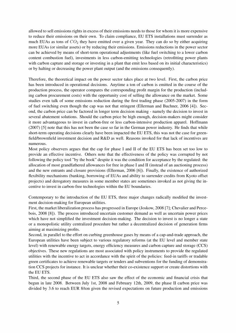
The two main processes for carbon price found in the literature on investment decision under carbonprice uncertainty so far are (1) the Geometric Brownian Motion (GBM) which is the price process ba-sically used for stocks and (2) a typical mean-reverting (MR) process, the Ornstein-Uhlenbeck model.Those price processes are sometimes completed by adding jumps to the processes to reflect abruptchanges in climate policy6. Table 1 surveys price processes used for carbon prices found in the literatureas well as fitting methods and data used.

Most authors have resorted to the GBM form to model the price of carbon. This is the typical formchosen for equity prices in option pricing model and implicitly makes an assumption of exponentialprice growth. In a policy-oriented study of investments under climate policy uncertainty, Blyth et al.(2007) [26] and Yang et al. (2008) [34] model the price of carbon as a GBM. Yang and Blyth (2007)[27] further improve their modeling of carbon price by simulating possible carbon price shocks thatwould represent policy-related events by adding a jump feature to the stochastic modeling (only onceten years from when the initial investment decision can be first taken). The GBM is fitted using a mix ofIEA projections and judgmental input.In an application to optimal rotation period for forest valuation, Chladna (2007) [35] resorts to a GBMfitted with the IIASA MESSAGE model. Szolgayova et al. (2008) [36] and Fuss et al. (2008) [24]assume that, while the electricity price is suggested to follow a mean-reverting process, the carbon pricefollows a GBM process. Again, the data used to parameterize the GBM comes from IIASA’s GGI Sce-nario database and originally refers to the shadow price of emissions. Fuss et al. (2009) [25] use thesame GBM to model the price of carbon but also add a jump process to reflect policy changes over avery long-term horizon (150 years). The size of jumps are drawn from an underlying GBM.Abadie and Chamorro (2008) [18] resort to a stochastic model of carbon prices to evaluate the prospectsof carbon capture investments in Spain. While all the other papers surveyed have been fitted using eithermodel projections or judgmental input, they model carbon prices using a a typical GBM fitted with EUETS Futures contracts data. Hence, they provide a risk-neutral version of GBM functional form explic-itly taking into account a Futures market risk premium. They estimate the parameters using a Kalmanfilter procedure with EUA Futures prices between January 2006 and October 2007.

In the literature, the choice of a mean-reverting price model is an alternative to the GBM which hasthe drawback to allow wider price developments over time (the variance of which grows infinitely) than

6Other authors have suggested other functional forms for carbon price modeling taking into account more detailed pricemovements like price spikes or regime switching. But those stochastic modeling are not initially done for investment decisionwhere the big picture matters the most but rather for derivatives pricing or short-term valuation purpose. See for example,Benz and Truck (2006) [32] for an application of regime-switching models and Daskalakis et al. (2007) [33] for applicationsof jump-diffusion models.

11

Tabl

e1:

Surv

eyof

carb

onpr

ice

stoc

hast

icm

odel

ing

Proc

ess

Star

tval

ueD

rift

Diff

usio

nJu

mp

Fitti

ngda

taE

xpec

ted

Ris

k-ad

just

edR

ever

sion

spee

dR

ever

sion

leve

lIn

stan

tane

ous

vola

tility

µc

µc−λ

cθ

c(P

c t)∗

σc

Aba

die

and

Cha

mor

ro(2

008)

GB

ME

UR

18/t

in20

07-

3.08

%-

-46

.83%

-13

25da

ilypr

ices

ofth

efiv

eFu

ture

sco

ntra

cts

mat

urin

gin

phas

eII

Chl

adna

(200

7)G

BM

USD

5/t

in20

103.

63%

--

-16

.60%

-II

ASA

ME

SSA

GE

mod

elFu

sset

al.(

2008

)and

Szol

-ga

yova

etal

.(20

08)

GB

ME

UR

5/t

5.68

%-

--

2.87

%-

GH

Gsh

adow

pric

esfr

omII

ASA

GG

Isc

enar

ioda

taba

se

Fuss

etal

.(20

09)

GB

Mw

ithan

dw

ithou

tG

BM

jum

p

USD

5/t

5.00

%-

--

0to

30%

freq

uenc

yis

from

0to

20ye

ars

GH

Gsh

adow

pric

esfr

omII

ASA

GG

Isc

enar

ioda

taba

seY

ang

&B

lyth

(200

7);B

lyth

etal

.(20

07)a

ndY

ang

etal

.(2

008)

GB

Mw

ithPo

isso

nju

mp

undi

sclo

sed

undi

sclo

sed

--

-7.

75%

+/-

100%

size

and

once

10ye

ars

from

now

Inor

der

tofo

llow

IEA

scen

ario

proj

ectio

ns15

year

sfr

omno

w

Yan

g&

Bly

th(2

008)

MR

USD

15/t

in20

05-

-0.

14E

UR

15/t

and

15%

p.a.

50.0

0%-

Inor

der

tofo

llow

IEA

scen

ario

proj

ectio

ns15

year

sfr

omno

wL

auri

kka

&K

oljo

nen

(200

6)M

RE

UR

7/t

in20

05-

-0.

20E

UR

20/t

orE

UR

1/t

in20

13

10or

40%

-ju

dgem

enta

linp

ut

12

mean reverting models. While models based on GBM have been used for tractability and ability toobtain closed-form expressions readily analyzable, mean reversion reflects the long-term equilibrium ofproduction and demand. Laurikka and Koljonen (2006) [23] model the natural logarithm of the priceof carbon allowances as a simple mean-reverting Ito process, namely an Ornstein-Uhlenbeck process(continuous state and discrete time). The authors assign two different values to the long-term price level(by 2013) depending on the scenario taken: EUR 20/ton in a high scenario and EUR 1/ton in a low pricescenario. Similarly, the variance parameter can take the value of 10% (low volatility scenario) or 40%(high volatility scenario). For fitting the model they use a starting price of EUR 7/ton based on earlyforward transaction prices reported by Point Carbon in 2004. Laurikka (2005) [22] suggests a simulationmodel which can simultaneously deal with multiple stochastic variables (emission allowances, electric-ity and fuels) to estimate the value of flexibility. Again, the stochastic processes used in the simulationmimic the simplest mean-reverting process (the Ornstein-Uhlenbeck process). It is important to remarkthat both studies were designed prior to the entry into force of the EU ETS.

When it comes to modeling the price of carbon, we contend it is more judicious to model the priceof carbon as a mean-reverting process along a linear trend for three main reasons7.First, we argue that carbon price long-term price drivers (the supposedly declining cap feature of thecap-and-trade policy, economic cycles oscillating around a long-term economic growth trend and tech-nological abatement options availability) are such that a mean-reverting around a trend makes sense.Second, even though there is no mean-reverting level as such, stakeholders actions should ensure notmuch price deviation (as would be implied by modeling the price of carbon as a GBM for instance) fromlong-term equilibrium. On the one hand, there are forces that would strive to prevent the price of carbonfrom reaching extremely high level. Too high a price is the sign of a cap level hardly compatible witha healthy economic activity8. On the other hand, there are forces eager to see the price of carbon reacha minimum threshold9. As such, market phases negotiations are the occasion to reset the rules in orderto adjust any fundamental flaw in the market design (like the implied ban on banking between phaseI and II during the trial phase). This is achieved on the regulator side by modifying the cap and otherelements of policy design (flexibility, derogations, etc.). On the regulated side, lobbying, pressuring andlegal challenges are the tools of the trade.Third, commodities have often been modeled as MR processes (Pindyck, 1999 [37] and Schwartz, 1997[38]) allowing to reflect some long-term cost of production, extraction or abatement. Even though itwas argued that the GBM was as good as a MR process when applied to a ROA framework, the currentcarbon spot prices are so remote from what a long-term equilibrium should be that a GBM would notbe appropriate. A quick look at other mandatory emissions markets (SO2 and NOx markets in the US)long term price evolution confirms our intuition of mean-reverting prices. The strong link with otherenergy commodity markets known for being mean-reverting goes in the same direction. Regarding theSO2 and NOx markets, it appears that price mean-reverted around a downward trend which can beinterpreted as technological breakthroughs to allow for emissions reduction and their penetration among

7Of course, it is ultimately each decision maker’s task to resort to the price process he deems the most appropriate. Thesame comment applies to the fitting of the process retained.

8The effect on the economy and society could be disruptive (insufficient power generation capacity, loss of internationalcompetitiveness for industries subject to carbon leakage, etc.). There exist a non-observable upper bound for the price ofcarbon reflecting the acceptability of compliance buyers above which their survival would be at stake (exit threshold).

9In this respect: the regulators (the EC and EU Member States) are urged to implement successfully the policy to justifytheir legitimacy to act as such. So are the politics who mandated the regulators and the international community pressuring theEU Member States to respect the engagement to reduce carbon emissions. NGOs and carbon market observers would monitorthe evolution of carbon price and would publicly advocate for environmental consciousness in case things go wrong. Carbon-reducing and carbon-neutral technology developers are concerned with keeping the incentive to maintain the developmentof such technologies and ensuring commercial prospects thereafter or own compliance prospects. Finally, regulated entitiesthemselves would push for meaningful carbon prices as a way to establish barriers to entry or at least increase the cost to enterthe market.

13

compliance buyers.

We now turn to the carbon price modeling retained. Let pct denote the spot price of a carbon emissionallowance (in EUR/tCO2) at time t. We assume that the pct is a continuous state stochastic variablefollowing an exogenous mean-reverting continuously-valued process with a linear trend and constantvolatility (one-factor model based on the log spot price from Lucia and Schwartz, 2000 [39]):

ln(pct) = hct

∗ +Xct

hct∗ = αc + βc.t (linear deterministic trend)

dXct = −θc.Xc

t .dt+ σcdW ct

In which, the log of the spot carbon price is expressed as the sum of (1) a totally predictable deterministicfunction of time (hct

∗) and (2) a diffusion stochastic process (Xct ) and where:

• θc is the constant mean reversion speed for the log of the carbon price;

• hct∗ = αc + βct is the linear trend for the log of the price of carbon (not a constant as in theOrnstein-Uhlenbeck model);

• σc represents the constant volatility of the instantaneous log-price variation;

• W ct is a standard Brownian motion for the log of the carbon price (providing unexpected price

shocks).

The linear trend for the price of carbon can be interpreted as the long run price depending on time. In ourmodel, this reflects future demand for abatement and future abatement options available in the marginalabatement cost curve.

Given our risk-neutral framework, we express the price of carbon according to:ln(pct) = hct

∗ + Xct

hct∗ = αc + βc.t (linear deterministic trend)

dXct = θc.(−λc.σc

θc − Xct ).dt+ σcdW c

t

Where the market price of risk for carbon, λc, is assumed to be a constant and the hat superscript usedhere denotes the move from the real world to the risk-neutral world.

Finally, we note that compliance with the EU ETS is most likely to be achieved by means of forwardtransactions thereby reflecting expectations and adjustments regarding emissions levels and availabilityof compliance assets. We assume that emissions allowances are purchased with annual forward or Fu-tures contracts10. We decide now of the transaction terms and exchange cash versus allowances at theconvened price at the maturity date.

Therefore, following Lucia and Schwartz (2000 [39]), we determine the forward price of carbon (nowfor a maturity T ):

F c0,T = EQ0 (P cT )

= exp[hcT∗︸︷︷︸

1

+ (ln(pc0)− hc0∗).e−θ

c.T︸ ︷︷ ︸2

−λc.σc

θc.(1− e−θc.T )︸ ︷︷ ︸

3

+(σc)2

4.θc.(1− e−2.θc.T )︸ ︷︷ ︸

4

]

10Note that since we use a constant discount rate, there is no difference between both types of contracts [39].

14

In which, the log of the forward price is comprised of11:

1. a deterministic trend component at time T ;

2. the spot price deviation from trend at t=0 multiplied by an adjustment/discount factor;

3. the mean-reverting level of the detrended process multiplied by one minus the adjustment factor;

4. the ratio of carbon price variance to its mean-reverting level multiplied by one minus twice theadjustment factor.

(3) The prices of electricityThe literature on the stochastic modeling of electricity prices (Geman, 2006 [40]; He, 2007 [2]) identifiesthat power prices have the following characteristics:

• High spot price volatility and volatility clustering effect (periods of high volatility tend to befollowed by similar periods);

• Mean reversion to the marginal cost of production (like most commodities);

• Seasonality (intraday, weekly and annual);

• Price jumps reflecting supply shocks (power plant outage) or unexpected demand;

• Market specific prices (reflecting the existing generation mix, demand profile and incentive poli-cies).

These characteristics pertain most to spot prices. There are two major way to model power spot pricesusing reduced-form models (i.e. directly modeling the time series, thereby avoiding to build an equilib-rium model). First, single factor models are the simplest type of reduced-form models12. They basicallyfeature the drift and diffusion components aforementioned. Second, two-factor models build on theprevious category and intend to complete the analysis by giving a stochastic behavior to one of the com-ponent of the single factor models (drift or diffusion)13.

Given that the spot market in Europe is almost exclusively an adjustment market (the real options liter-ature involving power prices reflects largely a focus on derivatives pricing), we assume that the powerplants that would be built would sell their production using exclusively forward transactions. This isquite realistic in the light of current European utilities practice. This basically means that we reduce thevolatility, drop the seasonality and price jump features compared to spot price modeling and resort to asingle factor model taking into account mean-reversion.

While the price of a ton of carbon is de facto EU-wide, it is not that simple for the price of a MWhgenerated and sold. The price of a MWh fundamentally depends on the power plant status in the gen-eration merit order related to a given demand source (country-wide most often) and for a given time.Given the power plant investment options suggested in the next section and more exactly the capacity,availability and competing power plants, the plant should either operate as a peakload or as a baseload

11Note that too high a mean-reversion speed makes forward/Futures prices identical across several process generation - thetrend component having an overwhelming influence over the rest.

12They are composed of Arithmetic Brownian Motion, Geometric Brownian Motion, the Ornstein-Uhlenbeck model, theGeometric Ornstein-Unhlenbeck model (in which the logarithm of the price follows the Ornstein-Uhlenbeck model) and theInhomogeneous Geometric Brownian Motion (which captures both the mean reversion and the price proportional characteris-tics of electricity prices).

13Stochastic volatility, stochastic long-term equilibrium price, etc. This category also features attempts to split short-termbehavior from long-term behavior, jump-diffusion models and regime-switching models.

15

plant. In our modeling environment, we assume that the CCGT, pulverized coal and IGCC plants wouldoperate as peakload plants and sell their power at peakload forward prices (ppt ). Conversely, the nu-clear plant would operate as a baseload plant and sell its power at baseload forward prices (pbt). Wesuggest modeling baseload and peakload power prices as mean-reverting processes with a linear trend(just like we did for carbon). The modeling should remain the same - only the fitting of parametersshould change. Additionally, sale of power generated by renewable energy sources often benefits froman incentive regime, be it tradable green certificates as in the UK or feed-in tariffs as in France. Forthe wind offshore investment alternative considered, we assume that the power generated can be sold atfeed-in tariffs (pft ) over the applicable period: EUR 130/MWh for the first ten years and EUR 64/MWhfor the remaining 10 years reflecting the current French feed-in tariffs14.

Further, it should be acknowledged that the introduction of the EU ETS has hardly been neutral onthe electricity prices15. We thus need to account for the linkages among the price processes. In theliterature, two approaches have been suggested.On the one hand, carbon and power stochastic prices can be positively correlated to account for the rela-tionship between those prices. Szolgayva et al. (2008) [36] and Fuss et al. (2008) [24] explicitly allowfor some passthrough via a positive correlation between the noises of the electricity and the carbon priceprocesses. The increments of the Wiener processes of electricity and carbon are assumed correlated at0.7. They assert that the positive value is implying that disturbances in the carbon price are positivelyreflected in those of electricity. In Laurikka and Koljonen (2006) [23], the price of carbon allowanceis modeled jointly with the price of baseload electricity using a quadrinomial tree. The relationship be-tween the two prices is summarized in a correlation factor which can take the value of either 0 or 0.5. Acausality study of carbon, electricity, coal, gas and stock prices (Keppler and Mansanet-Bataller, 2009[41]) identifies that the Granger causality relationship between carbon and electricity prices evolves fromphase I to phase II. This could support the idea that simulation of power and carbon prices need to bemore refined than a constant correlation factor16.On the other hand, some authors explicitly modeled the level of passthrough (see Laurikka and Koljonen,2006 [23]). Consequently, the estimated price of baseload electricity is the simulated baseload price inthe absence of an emissions trading scheme (a counterfactual or business-as-usual - BAU - price in otherwords) to which is added the price of carbon times an estimated transformation factor. That approachhas the advantage to account for the potentially directional relationship from carbon prices to electricityprices while having the disadvantage to require the modeling of a forward-looking BAU electricity price.Laurikka and Koljonen (2006) [23] estimate that transformation factor between 0.22 and 0.77 dependingupon the prevailing BAU electricity price.

We now turn to the modeling retained for peakload and baseload prices. The approach retained issimilar to that of the price of carbon. Moving directly to the risk-neutral world:

ln(ppt ) = hpt∗ + Xp

t (for peakload power spot price)hpt

∗ = αp + βp.t (linear deterministic trend)dXp

t = θp.(−λp.σp

θp − Xpt ).dt+ σpdW p

tln(pbt) = hbt

∗ + Xbt (for baseload power spot price)

hbt∗∗ = αb + βb.t (linear deterministic trend)

dXbt = θb.(−λb.σb

θb − Xbt ).dt+ σbdW b

t

14For investment renewal 20 years from initial investment, we assume that the support scheme has ended and that baseloadpower prices apply for valuation purpose.

15For instance, refer to the BundesKartellamt decisions in Germany on RWE & E.ON alleged passthrough as early as 2005.16We leave this point to further research.

16

where:

• θp and θb are the constant mean-reversion speeds for the log of peakload and baseload electricityprice;

• hpt∗ = αp + βp.t is the linear trend for the log of the price of peakload power;

• hbt∗ = αb + βb.t is the linear trend for the log of the price of baseload power;

• σp and σb representing the constant volatility of the instantaneous log-price variation for peakloadand baseload electricity prices;

• λp and λb are the market prices of risk for the log of the peakload and baseload power prices;

• W pt andW b

t are standard Brownian motions for the log of the peakload and baseload power prices.

We now express forward prices for the stochastic processes of power price:

F p0,T = EQ0 (P pT ) (for peakload power forward price)

= exp[hpT∗ + (ln(pp0)− hp0

∗).e−θp.T − λp.σ

p

θp.(1− e−θp.T )

+(σp)2

4.θp.(1− e−2.θp.T )]

F b0,T = EQ0 (P bT ) (for baseload power forward price)

= exp[hbT∗

+ (ln(pb0)− hp0∗).e−θ

b.T − λb.σb

θb.(1− e−θb.T )

+(σb)2

4.θb.(1− e−2.θb.T )]

(4) Correlation among stochastic state variablesWe also ensured that single price process generation would not deviate from the basic relationship amongthem. We therefore used constant correlation factors among the increments of the three Brownian mo-tions involved (ρp,c, ρb,c and ρp,b).

(5) The price of fossil fuelsIn order to simplify the model used and strictly focus on carbon price uncertainty, we assume that fuelprices follow deterministic paths (that is, we know for sure the future prices of fuels).

Coal and natural gas are modeled as deterministic state variables consistent with the IEA 2008 price sce-nario assumptions (IEA, 2008 [42]). The IEA price scenario assumptions are the results of a top-downassessment of prior needs to encourage sufficient investment in supply and meet projected demand by2030. In particular, it is assumed that the price of coal remains at USD 120/ton17 of coal between 2010and 2015 and linearly goes down to USD 110/ton of coal as new mining and transportation capacitybecomes available. We further assume that coal prices remains at that level for the rest of our studyhorizon.Similarly, the price of natural gas is expected to follow the following path in USD/MMBTU: 11.15 in2010, 11.50 in 2015, 12.71 in 2020, 13.45 in 2025 and 14.19 in 2030. A linear interpolation betweentarget prices and current prices is generated for the missing dates. Beyond 2030, we apply an annual

17We assume that 1.3705 EUR/USD consistent with the average FX rate in 2007 (WEO assumptions are expressed in 2007USD) according to the ECB.

17

Figure 2: Price trajectories for fossil fuels (IEA, 2008)

60,00

80,00

100,00

120,00

140,00

COAL (USD/tons)

NATGAS (USD/MMBTU)

-

20,00

40,00

20

10

20

13

20

16

20

19

20

22

20

25

20

28

20

31

20

34

20

37

20

40

20

43

20

46

20

49

20

52

20

55

20

58

20

61

20

64

growth rate of 1.077% reflecting the average growth rate between the last two target dates. Figure 2illustrate both price trends.

Regarding uranium, we used a per MWh cost assumption instead of a dedicated price modeling giventhat (1) nuclear power plants either are supplemented with long-term uranium procurement contractsor the turnkey agreements incorporate such long-term contracts to begin with and (2) the volatility ofnuclear ore prices and power plant valuation sensitivity to them is quite low. In particular, we assumeda nuclear fuel cost of EUR 15/MWh.

(6) Time and discount rateWe assume an investment window of 10 years starting from now (t=0). The frequency of decision pointsin time is annual (t ∈ ‖0; 10‖). Given that power plant lifetime goes up to 40 years and building timecan go up to 5 years, the horizon for simulations reaches 56 years.The investment window retained makes our model a string of Bermudan call options with lookback fea-tures given that exercise is limited to certain dates within the life of the option and that the exercise doesnot necessarily kill the ability to subsequently invest in other power plants (budget permitting).The risk-free discount rate used, r, is set at 4%.

2.2.2 The choice variable

There is a single discrete choice variable, namely the decision to invest in power plants. At any decisionnode in time, we may invest or wait one more period (for instance to see how the carbon price evolves).Should we wish to invest, we can invest in one power plant or a ”basket” of power plants. The invest-ment alternatives are building a CCGT power plant (incur IG), a supercritical pulverized coal powerplant (incur IK), an IGCC power plant (incur II ), a nuclear power plant (incur IN ), an offshore windpower plant (incur IW ) or a combination of those. Once the initial investment cost has been incurred,we are entitled cash flows over the lifetime of the power plant.

Power plant characteristics including capital cost estimates are taken from the NEA, IEA and OECDprojections (2005) [43] for European countries and from IEA (2008 [42]) when more up-to-date figures

18

make more sense18.For the purpose of the study, we considered five generation technologies:

• CCGT plants basically characterized by a moderate capital cost, high and volatile fuel procure-ment cost and an average carbon compliance cost;

• Supercritical pulverized coal plants characterized by a higher capital cost than CCGT plants, lowerfuel procurement cost but higher carbon compliance cost than CCGT’s. These power plants canbe further retrofitted with CCS modules;

• IGCC power plants which gasification process makes it possible to switch burning fuel dependingon relative costs, especially in the light of carbon emissions factors;

• Nuclear power plants characterized by a very high capital cost but a low fuel procurement costand no carbon compliance cost;

• An offshore19 wind park characterized by a high capital cost (relative to capacity) but no fuelprocurement cost and no carbon compliance cost. Additionally, we assume that investment inthese technologies is favored since they benefit from feed-in tariffs;

For each of those power plants, we report the value range for investment, emissions and technical data.

The CCGT plant total investment cost (initial investment cost and operation and maintenance cost overthe life of the plant discounted at 8.5%) amounts to some EUR 914 million (see table 14 in annex forolder cost estimates and value range in NEA, IEA and OECD, 2005 [43]). The plant takes 3 years to bebuilt and will operate during 40 years. The thermal capacity of the power plant is set at 900 MW andits thermal efficiency is set at 59%. It is assumed that the plant will deliver power 42.5% of the year(3,723 hours). Based on this availability factor, the expected daily output for the power plant is 9,180MWh (3.35 GWh per annum). Regarding carbon emissions, the emissions factor of the CCGT plant isassumed at 0.353 tCO2/MWh (which amounts to 1.168 MtCO2 on annual basis).The pulverized coal plant represents a typical investment in a supercritical coal-fired plant (see table 15in annex for value range). The pulverized coal unit total investment cost amounts to circa EUR 1,632million. Again, the lifetime of the plant is set at 40 years and it only takes 3 years to build the plant. Thethermal capacity of the plant is set at 800 MW and its thermal efficiency at 46%. With an availabilityfactor of 42.5%, this represents 8.160 MWh on a daily basis (2.98 GWh p.a.). The emissions factor ishigher than for the CCGT plant and reaches 0.728 tCO2/MWh generated (equivalent to 2.168MtCO2

each year).We also consider an integrated gasification combined cycle (IGCC) as an alternative to the pulverizedcoal plant (see table 16 in annex for value range). The IGCC plant total investment cost amounts tocirca EUR 1,298 million. Lifetime of the plant is set at 40 years and 3 years are required to commissionthe plant. The thermal capacity of the plant is set at only 450 MW and its thermal efficiency is at 46%.With an availability factor of 42.5%, this represents 4.589 MWh on a daily basis (1.67 GWh p.a.). Theemissions factor is lower than the pulverized coal plant’s but still higher than the CCGT’s and reaches0.656 tCO2/MWh generated (equivalent to 1.099 MtCO2 each year).The nuclear power plant is the first of the two carbon-free investment alternatives (see table 17 in an-nex for value range). The total investment cost (including discounted nuclear waste decommissioning)amounts to EUR 5,896 million. The plant takes 5 years to be built and will operate over 40 years. The

18Please note that recently power plant investment costs have been strongly rising (cost of materials, components, laborand lack of skilled engineers). We estimate that investment costs have more than doubled among the generation technologiesconsidered in our study.

19For the sake of comparison among generation technologies in terms of generation capacity.

19

thermal capacity of the plant is 1,590 MW. With an availability factor of 85%, this represents 32.438MWh on a daily basis (11.84 GWh p.a.).The offshore wind plant is the other carbon-free investment alternative (see table 18 in annex for valuerange). The total investment cost reaches EUR 792 million. The wind farm takes 1 year to be built andwill operate over 20 years. The average load factor of the wind farm is 42% and the capacity is 300 MW.This amounts to a potential 3.287 MWh on a daily basis (1.20 GWh p.a.).

Table 2 summarizes our assumptions for the power plant investment alternatives.

Table 2: Power plant assumption dataCCGT Plant PC IGCC Nuclear Wind

Construction length - in years 3 3 3 5 1Lifetime - in years 40 40 40 40 20

Thermal capacity - in MWe 900 800 450 1590 300Thermal efficiency - in % 59 40 46 36 -Average load factor - in % - - - - 42

Expected annual output - in GWh 3.35 2.98 1.67 11.84 1.20CO2 emissions factor - in tCO2/MWh 0.353 0.728 0.656 0.000 0.000Annual carbon emissions - in MtCO2 1.168 2.168 1.099 0.000 0.000Total investment costs - in EUR million 914 1632 1298 5896 792

Given an initial budget of EUR 5.9 billion, this implies that the budget variable can take any of thefollowing values:

bt ∈ { 4︸︷︷︸After nuclear x1

; ...; 5900︸︷︷︸Untapped

} , ∀t

and the control variable:

xt ∈ { 0︸︷︷︸Wait

; 792︸︷︷︸Wind x1

; 914︸︷︷︸CCGT x1

; ...; 5896︸︷︷︸Nuclear x1

} , ∀t

2.2.3 The functions

The reward functionThe reward function ft identifies immediate reward from undertaking a specific choice at time t. Thisreward corresponds to the net present value (NPV) of given investment combination alternatives. Notethat the value taken by this function depends on market prices conditions, the timing of investment, thebudget level and the investment combinations decided upon. We identified 121 unique combinations of

20

generation technologies20.

ft(bt, xt, St) =

0 for xt = 0,NPV G

t for xt = IG,

NPV Wt for xt = IW ,

NPV It for xt = II ,

NPV Kt for xt = IK ,

2.NPV Gt for xt = 2.IG,

...,

NPV Nt for xt = IN .

s.t. xt ≤ bt ,∀t

Where the NPV for a given technology at time t is the sum of discounted annual cash flow minusinvestment cost:

NPV techt =

t+buildtech+lifetech∑j=t+buildtech

[Πtechj .e−r.j ]− Itech

In which:

• ΠGt = qG.[(

P24j=1 F

pt−j/12, t

24 )−pgt /TEG−(P24

j=1 Fct−j/12, t

24 .EFG)] annual cash flow for the CCGTplant;

• ΠWt = qW .pft annual cash flow for the wind power plant benefiting from feed-in tariffs (first 20

years);

• ΠWt = qW .[

P24j=1 F

bt−j/12, t

24 ] annual cash flow for the wind power plant after having benefitedfrom feed-in tariffs (next 20 years);

• ΠIt = qI .[(

P24j=1 F

pt−j/12, t

24 ) − pkt /TEI − (P24

j=1 Fct−j/12, t

24 .EF I)] annual cash flow for the IGCCplant;

• ΠKt = qK .[(

P24j=1 F

pt−j/12, t

24 ) − pkt /TEK − (

P24j=1 F

ct−j/12, t

24 .EFK)] annual cash flow for thepulverized coal plant;

• ΠNt = qN .[(

P24j=1 F

bt−j/12, t

24 )− 15] annual cash flow for the nuclear plant;

And:

• qG, qW , qI , qK , and qN are the annual quantities of electricity (inMWh) produced by the CCGT,wind, IGCC, pulverized coal and nuclear plant respectively;

• F ct−j/12, t, Fpt−j/12, t, and F bt−j/12, t are the forward prices (agreed upon at t − j/12 and settling

in t) for carbon and electricity (peakload and baseload) respectively;

• pgj , pkj and pfj are the average annual spot prices for natural gas and coal and the feed-in tariff foroffshore wind;

20In case the condition xt ≤ bt is not respected, we will assume, for valuation purpose, that ft(bt, xt, St) takes the value of−∞.

21

• TEI , TEK and TEG are the thermal efficiencies of the IGCC, pulverized coal and CCGT plantsrespectively;

• EF I ,EFK andEFG are the carbon emissions factors (in tCO2/MWh) of the IGCC, pulverizedcoal and CCGT plant respectively;

• r corresponds to the zero-coupon rate (the risk-free rate);

• lifeG, lifeW , lifeI , lifeK and lifeN are the life times of the CCGT, wind, IGCC, pulverizedcoal and nuclear plant respectively;

• buildG, buildW , buildI , buildK and buildN are the construction times of CCGT, wind, IGCC,pulverized coal and nuclear plant respectively;

We acknowledge that the utility, unwilling to remain exposed to price risk, would engage in forwardtransaction to secure future cash flows. We assume a monthly risk management meeting in which theutility hedge 1/24 of the next two years’ expected production for both power and carbon prices. Thisseems a reasonable assumption in light of calendar contracts liquidity on market places and market prac-tice as indicated by European utilities annual reports21. This implies that the price at which the powerproduction is sold at time t is not the contemporary spot price but rather an average of the last two yearscalendar forward prices (on the basis of a monthly transaction for 1/24 of the annual production in yeart) resulting in a smoother prices less exposed to high spot price volatility.

The value functionThe principle of optimality applied to our discrete time mixed states decision models yield Bellman’srecursive functional equation. Here, Vt denotes the maximum attainable sum of current and expectedfuture rewards given that the processes are in states bt and St in period t:

Vt(bt, St) = maxxt

ft(bt, xt, St)︸ ︷︷ ︸immediate reward component

+ e−r.EQt [Vt+1(bt − xt, St+1)︸ ︷︷ ︸discounted expected reward component

]

,∀ bt and ∀ St (1)

The first element of the Bellman equation corresponds to the immediate benefits (f ) while the secondelement corresponds to the discounted expected future benefits (knowing St).This latter component is also known, in the financial option terminology, as the continuation value andis estimated by OLS following the method suggested by Longstaff ans Schwartz (2001, [14]).

The post-terminal value functionSince we are in a finite horizon problem, the investor cannot invest after T periods but may earn a fi-nal reward VT+1 which corresponds to the remaining immediate investment opportunity of the possibleinvestment ”baskets”. We assume no continuation value after T , so that at expiration:

VT (bT , ST ) = maxxT

fT (bT , xT , ST )︸ ︷︷ ︸immediate reward component

,∀ bT and ∀ ST (2)

In our backward recursion setting, this will be our starting point. With VT , we can find recursively VT−1

for all states (bT , ST ). With VT−1, we can find recursively VT−2 for all states (bT−1, ST−1) and so onuntil V0(b, S0) is derived and the optimal policy established since there is no uncertainty at t=0 so thatwe can work our way forward into the recursion.

21RWE financial statements for 2008 indicates that, in fiscal year 2008, the utility actually hedged nearly 100% of itsexpected power production for 2009 and approximately 70% for 2010 (by selling power using forward transaction).

22

2.3 Calibrating the stochastic processes

It should be reminded that once the price process has been chosen, a critical step is the calibration thereof.In addition to that, it should be stressed that usually at least 30 years of historical data is required in orderto properly calibrate a model (Dixit and Pindyck, 1994 [15]; Keppler et al., 2006 [44]). In our case, thisis obviously impossible (in the carbon and power prices cases). Hence, the initial parameters estimatedshould suffice and would constitute our base case. Later, we will look at the sensitivity of the investmentsdecided upon given the parameters.

2.3.1 Fitting the stochastic price of carbon

The literature shows that the calibration of the carbon price processes is a mix of inputs from economet-ric analysis of historical data, model output (like the IIASAs GGI Scenario database) and judgmentalinput be it a shadow price (valeur tutelaire du carbone in France for instance) or academic and profes-sional expert price elicitation survey (like in Sekar, 2005 [21] and Bohm et al., 2007 [19]).

We first fit the process with historical data using econometric techniques. We will discuss the eco-nomic meaning around those parameters in the later section on parameter sensitivity study.

2.3.2 Fitting the stochastic prices of power

2.3.3 Estimating correlations among stochastic processes

We estimated correlations between the spot price of baseload electricity, peakload electricity and carbon(ρp,c, ρb,c and ρp,b) using time series employed for fitting the price processes (see table 3 for the estimatedcorrelations).

Table 3: Correlation among stochastic price processesρx,y dW p dW b dW c

dW p 1.00 0.95 0.49dW b - 1.0 0.55dW c - - 1.0

3 Illustrative cases

In this section, we present simpler case studies to grasp how (1) the capital rationing constraint and (2)the price uncertainty can be handled.

3.1 3-period 2-technology deterministic case

In order to illustrate how to solve the capital rationing issue, we detail calculations for a 3-period deter-ministic case. We consider two technologies, A and B, with investment costs of IA and IB irrespectiveof time. We are constrained by a budget of b. We may invest in a combination of technologies now, nextyear or two years from now. To do so, we incur investment costs and benefit from resulting NPVs.We assume the following: e−r = 0.909; b = 1,000; IA = 400; IB = 700; NPV A

t = 200 , ∀t; NPV Bt =

300 for t = {0; 1} and NPV Bt = 500 for t=2.

Finding the allowed investment combinations

23

The first step entails determining what are the allowed investment combinations. We are constrained bythe capital rationing so that xt ≤ bt , ∀t.Denoting QA and QB , the quantity of technologies we invest in, we must satisfy:

xt = IA.QA + IB.QB ≤ bt

Here, we easily see that the control variable can take the following values:

xt ∈ { 0; IA; IB; 2.IA}∈ { 0; 400; 700; 800}

And the budget can therefore take the following values:

bt ∈ { b− 2.IA; b− IB; b− IA; b}∈ { 200; 300; 600; 1000}

At t=2We start from the last decision node at t=2. The value function takes the following form:

V2(b2) = maxx2

{f2(b2, x2)}

At the last decision node, we have no continuation value since unused budget is assumed to have novalue. We consider all the possible budget levels and determine the value function accordingly22:

V2(b− 2.IA) = maxx2

{f2(b− 2.IA, 0)

}= 0 with x∗2=0.

V2(b− IB) = maxx2

{f2(b− IB, 0)

}= 0 with x∗2=0.

V2(b− IA) = maxx2

{f2(b− IA, 0); f2(b− IA, IA)

}= max

x2

{0;NPV A

2

}= max

x2

{0; 200}

= 200 with x∗2=IA.

V2(b) = maxx2

{f2(b, 0); f2(b, IA); f2(b, IB); f2(b, 2.IA)

}= max

x2

{0;NPV A

2 ;NPV B2 ; 2.NPV A

2

}= max

x2

{0; 200; 500; 400}

= 500 with x∗2=IB .

At t=1We move one step back in time to t=1. The value function now takes the following form since there is acontinuation value component involved:

V1(b1) = maxx1

{f1(b1, x1) + e−r.V2(b1 − x1)

}22For the first two budget levels, only one possibility remains, that is to do nothing/wait. The three other possible choices

make us exhaust the budget limit.

24

We consider all the possible budget levels and determine the value function accordingly:

V1(b− 2.IA) = maxx1

{f1(b− 2.IA, 0) + e−r.V2(b− 2.IA)

}= 0 with x∗1=0.

V1(b− IB) = maxx1

{f1(b− IB, 0) + e−r.V2(b− IB)

}= 0 with x∗1=0.

V1(b− IA) = maxx1

{f1(b− IA, 0) + e−r.V2(b− IA); f1(b− IA, IA) + e−r.V2(b− 2.IA)

}= max

x1

{0 + e−r.NPV A

2 ;NPV A1 + 0

}= max

x1

{182; 200}

= 200 with x∗1=IA.

V1(b) = maxx1

{f1(b, 0) + e−r.V2(b); f1(b, IA) + e−r.V2(b− IA);

f1(b, IB) + e−r.V2(b− IB); f1(b, 2.IA) + e−r.V2(b− 2.IA)}

= maxx1

{0 + e−r.NPV B

2 ;NPV A1 + e−r.NPV A

2 ;NPV B1 + 0; 2.NPV A

1 + 0}

= maxx1

{455; 381; 300; 400}

= 455 with x∗1=0.

At t=0We move one step back in time to t=0 (now). The value function again takes the following form:

V0(b0) = maxx0

{f0(b0, x0) + e−r.V1(b0 − x0)

}Compared to t=1 and t=2, we only have one possible budget level, b, the initial endowment.

V0(b) = maxx0

{f0(b, 0) + e−r.V1(b); f0(b, IA) + e−r.V1(b− IA);

f0(b, IB) + e−r.V1(b− IB); f0(b, 2.IA) + e−r.V1(b− 2.IA)}

= maxx0

{0 + e−2r.NPV B

2 ;NPV A0 + e−r.NPV A

1 ;NPV B0 + 0; 2.NPV A

0 + 0}

= maxx0

{413; 381; 300; 400}

= 413 with x∗0=0.

The optimal pathV0(b) represents the maximum value that can be attained in the investment framework considered. Theoptimal path represents the decisions that must be taken sequentially in order to realize that maximumvalue. At t=0, the optimal decision is to wait (x∗0=0), the budget remains intact. Moving forward in thetree, we look for V1(b) and again the optimal decision is to wait (x∗1=0). Moving to the last decision node,we look for V2(b) and find that the optimal decision is to invest in one unit of technology B (x∗2=IB).The maximum attainable gain is realized by purchasing one unit of technology B two years from now.A now-or-never DCF framework would have yield a myopic investment in two units of technology Anow, EUR 13 million less than accounting for the timing option.

3.2 3-period 2-technology stochastic case

We now add uncertainty to the NPV of one of the technologies. In particular, we generate eight pricepaths for one source of uncertainty (the price of baseload power). This source of uncertainty only per-tains to technology B. Technology A has the same NPV whenever we decide to invest: NPV A

t = 250

25

,∀t. Table 4 compiles the eight price paths generated for the source of uncertainty assumed here. Notethat the price of baseload power at t=0 is known for sure23. The set of stochastic state variables, Sit ,denotes here solely the price of baseload power at time t on price path i.

Table 4: Illustrative case - Price paths for baseload powerSi

t t=0 t=1 t=2 t=3 ... t=431 50.52 53.29 54.80 57.51 ... 150.892 50.52 54.05 55.92 58.43 ... 159.453 50.52 54.24 55.87 58.72 ... 154.304 50.52 53.20 56.18 59.57 ... 167.615 50.52 53.81 56.04 57.90 ... 151.146 50.52 54.69 57.89 59.35 ... 154.807 50.52 53.04 54.84 57.08 ... 153.148 50.52 53.88 57.08 59.80 ... 152.36

Based on those price paths, we obtain eight NPV paths for technology B. We denote NPV B,it , the NPV

of technology B at time t on path i. Table 5 presents the hypothesized eight NPV paths for technology B.

Table 5: Illustrative case - Implied NPV paths for technology BNPV B,i

t t=0 t=1 t=21 278 372 4612 495 598 6993 321 417 5084 751 865 9765 261 354 4446 573 674 7677 241 337 4308 502 597 686

The value function now takes the following form:

Vt(bt, Sit) = maxxt

{ft(bt, xt, Sit) + e−r.EQt [Vt+1(bt − xt, Sit+1)]

}, ∀i and ∀t.

And at expiration

VT (bT , SiT ) = maxxT

{fT (bT , xT , SiT )

},∀i.

At t=2We start from the last decision node at t=2. The value function takes the following form:

V2(b2, Si2) = maxx2

{f2(b2, x2, S

i2)},∀i.

23A high growth rate has been retained for illustrative purpose.

26

At the last decision node, we have no continuation value since unused budget is assumed to have novalue. We consider all the possible budget levels and determine the value function accordingly:

V2(b− 2.IA, Si2) = maxx2

{f2(b− 2.IA, 0, Si2)

}= 0 with x∗2=0 and ∀i.

V2(b− IB, Si2) = maxx2

{f2(b− IB, 0, Si2)

}= 0 with x∗2=0 and ∀i.

V2(b− IA, Si2) = maxx2

{f2(b− IA, 0, Si2); f2(b− IA, IA, Si2)

}= max

x2

{0;NPV A

2

}= max

x2

{0; 250}

= 250 with x∗2=IA and ∀i.

The untapped budget level case (b2=b) is the only one allowing investment in technology B and hencefeaturing uncertainty.

V2(b, Si2) = maxx2

{f2(b, 0, Si2); f2(b, IA, Si2); f2(b, IB, Si2); f2(b, 2.IA, Si2)

}= max

x2

{0; NPV A

2 ; NPV B,i2 ; 2.NPV A

2

}

In table 6, we detail the investment alternatives at t=2 when the budget is full and highlight in bold themaximum value and associated decision taken.

Table 6: Illustrative case - Decision nodes at t=2 and optimal decision for untapped budgetPath 0 NPV A

2 NPV B,i2 2.NPV A

2 x∗21 0 250 461 500 2.IA

2 0 250 699 500 IB

3 0 250 508 500 IB

4 0 250 976 500 IB

5 0 250 444 500 2.IA

6 0 250 767 500 IB

7 0 250 430 500 2.IA

8 0 250 689 500 IB

average 0 250 622 500 IB

In tables 7 and 8, we summarize the value functions and optimal decisions for each budget level andeach path at t=2.

Table 7: Illustrative case - Value function vs. budget level at t=2Path b2 = b− 2.IA b2 = b− IB b2 = b− IA b2 = b

1 0 0 250 5002 0 0 250 6993 0 0 250 5084 0 0 250 9765 0 0 250 5006 0 0 250 7677 0 0 250 5008 0 0 250 689

27

Table 8: Illustrative case - Optimal decision vs. budget level at t=2Path b2 = b− 2.IA b2 = b− IB b2 = b− IA b2 = b

1 0 0 IA 2.IA

2 0 0 IA IB

3 0 0 IA IB

4 0 0 IA IB

5 0 0 IA 2.IA

6 0 0 IA IB

7 0 0 IA 2.IA

8 0 0 IA IB

At t=1The value function now takes the following form:

V1(b1, Si1) = maxx1

{f1(b1, x1, S

i1) + e−r.EQ1 [V2(b1 − x1, S

i2)]}, ∀i.

Note that the exercise decision at t=1 cannot exploit knowledge of the future (i.e. the value taken at t=2)on a given path. We are not replacing a stochastic problem by 8 deterministic problems. Rather, weare regressing value functions discounted back at t=1 against the value of Sit . We are using our set ofscenarios to build an approximation of the conditional expectation continuation value component. Thatis the key idea of the Longstaff and Schwartz method. Note that we only do so when stochasticity isinvolved, i.e. when we may invest in technology B24.

We proceed like in the deterministic case by detailing the value function in t=1 for all the budget com-binations.

V1(b− 2.IA, Si1) = maxx1

{f1(b− 2.IA, 0, Si1) + e−r.EQ1 [V2(b− 2.IA, Si2)]

}= max

x1

{f1(b− 2.IA, 0, Si1) + e−r.V2(b− 2.IA, Si2)

}= 0 with x∗1=0 and ∀i.

V1(b− IB, Si1) = maxx1

{f1(b− IB, 0, Si1) + e−r.EQ1 [V2(b− IB, Si2)]

}= max

x1

{f1(b− IB, 0, Si1) + e−r.V2(b− IB, Si2)

}= 0 with x∗1=0 and ∀i.

V1(b− IA, Si1) = maxx1

{f1(b− IA, 0, Si1) + e−r.EQ1 [V2(b− IA, Si2)];

f1(b− IA, IA, Si1) + e−r.EQ1 [V2(b− 2.IA, Si2)]}

= maxx1

{f1(b− IA, 0, Si1) + e−r.V2(b− IA, Si2);

f1(b− IA, IA, Si1) + e−r.V2(b− 2.IA, Si2)}

= maxx1

{0 + e−r.NPV A

2 ;NPV A1 + 0

}= max

x1

{227; 250}

= 250 with x∗1=IA and ∀i.24In our general case, this will be almost always the case.

28

We move to the b1 = b case.

V1(b, Si1) = maxx1

{f1(b, 0, Si1) + e−r.EQ1 [V2(b, Si2)];

f1(b, IA, Si1) + e−r.EQ1 [V2(b− IA, Si2)];

f1(b, IB, Si1) + e−r.EQ1 [V2(b− IB, Si2)];

f1(b, 2.IA, Si1) + e−r.EQ1 [V2(b− 2.IA, Si2)]}

= maxx1

{f1(b, 0, Si1) + e−r.EQ1 [V2(b, Si2)];

f1(b, IA, Si1) + e−r.[V2(b− IA, Si2)];f1(b, IB, Si1) + e−r.[V2(b− IB, Si2)];f1(b, 2.IA, Si1) + e−r.[V2(b− 2.IA, Si2)]

}In our illustrative case, only one investment decision is problematic (do not invest/wait at t=1 in blue) andwe will approximate the expected continuation value by performing a linear regression of e−r.V2,i(b)against a set of basis functions for this decision. The basis functions retained in this example are the firstand second powers of the power price paths.We consider the following regression model:

e−r.EQ1 [V2(b, Si2)] ≈ φ2(b, Si2) = c0,1 + c1,1.Si1 + c2,1.(Si1)2 + ei

Table 9 compiles data for the regression (dependent and independent variables). The linear regression

Table 9: Illustrative case - Sample OLS regression dataPath e−r.V2,i(b) Si

1 (Si1)2

1 455 53.29 2,8402 635 54.05 2,9223 462 54.24 2,9424 887 53.20 2,8315 455 53.81 2,8966 697 54.69 2,9917 455 53.04 2,8138 624 53.88 2,903

yields the following25:

e−r.EQ1 [V2(b, Si2)] ≈ φ2(b, Si2) = 357, 959− 13, 302(Si1) + 123.77(Si1)2

Coming back to the value function, we replace the conditional expectation component by its approx-imation (in blue):

V1(b, Si1) ≈ maxx1

{f1(b, 0, Si1) + φ2(b, Si2); f1(b, IA, Si1) + e−r.[V2(b− IA, Si2)];

f1(b, IB, Si1) + e−r.[V2(b− IB, Si2)]; f1(b, 2.IA, Si1) + e−r.[V2(b− 2.IA, Si2)]}

≈ maxx1

{0 + φ2(b, Si2); NPV A

1 + e−r.NPV A2 ; NPV B

1 + 0; 2.NPV A1 + 0

}In table 10, we detail the investment alternatives at t=1 and highlight in bold the maximum value.

25To improve the quality of the linear regression and the computation speed in more complex cases, we may exclude pathsfavoring investments in technology A or waiting over investment in technology B for the linear regression estimation. Wewould therefore build on the moneyness criteria idea used for American option pricing in the Longstaff and Schwartz paper.We do not detail that here but will consider doing so in later sections / versions of this paper.

29

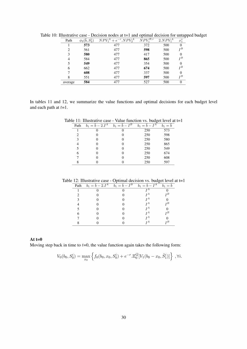
Table 10: Illustrative case - Decision nodes at t=1 and optimal decision for untapped budgetPath φ2(b, Si

2) NPV A1 + e−r.NPV A

2 NPV B,i1 2.NPV A

1 x∗11 573 477 372 500 02 561 477 598 500 IB

3 580 477 417 500 04 584 477 865 500 IB

5 549 477 354 500 06 662 477 674 500 IB

7 608 477 337 500 08 551 477 597 500 IB

average 584 477 527 500 0

In tables 11 and 12, we summarize the value functions and optimal decisions for each budget leveland each path at t=1.

Table 11: Illustrative case - Value function vs. budget level at t=1Path b1 = b− 2.IA b1 = b− IB b1 = b− IA b1 = b

1 0 0 250 5732 0 0 250 5983 0 0 250 5804 0 0 250 8655 0 0 250 5496 0 0 250 6747 0 0 250 6088 0 0 250 597

Table 12: Illustrative case - Optimal decision vs. budget level at t=1Path b1 = b− 2.IA b1 = b− IB b1 = b− IA b1 = b

1 0 0 IA 02 0 0 IA IB

3 0 0 IA 04 0 0 IA IB

5 0 0 IA 06 0 0 IA IB

7 0 0 IA 08 0 0 IA IB

At t=0Moving step back in time to t=0, the value function again takes the following form:

V0(b0, Si0) = maxx0

{f0(b0, x0, S

i0) + e−r.EQ0 [V1(b0 − x0, S

i1)]}, ∀i.

30

At t=0, we only have one possible budget level, b, the initial endowment.

V0(b, Si0) = maxx0

{f0(b, 0, Si0) + e−r.EQ0 [V1(b, Si1)];

f0(b, IA, Si0) + e−r.EQ0 [V1(b− IA, Si1)];

f0(b, IB, Si0) + e−r.EQ0 [V1(b− IB, Si1)];

f0(b, 2.IA, Si0) + e−r.EQ0 [V1(b− 2.IA, Si1)]}

= maxx0

{f0(b, 0, Si0) + e−r.EQ0 [V1(b, Si1)];

f0(b, IA, Si0) + e−r.V1(b− IA, Si1);f0(b, IB, Si0) + e−r.V1(b− IB, Si1);f0(b, 2.IA, Si0) + e−r.V1(b− 2.IA, Si1)

}= max

x0

{0 + e−r.EQ0 [V1(b, Si1)]; NPV A

0 + e−r.NPV A1 ;

NPV B,i0 + 0; 2.NPV A

0 + 0}

= maxx0

{e−r.EQ0 [V1(b, Si1)]; 477; NPV B,i

0 ; 500}

Now simply discounting all cash flows back to time t=0 and averaging over the eight sample paths,we get an estimate of e−r.EQ0 [V1(b, Si1)] 26. We obtain in table 13 the maximum value and associatedoptimal decisions:

Table 13: Illustrative case - Decision nodes at t=0 and optimal decision for initial budgetPath e−r.EQ

0 [V1(b, Si1)] NPV A

0 + e−r.NPV A1 NPV B,i

0 2.NPV A0 x∗0

1 521 477 278 500 02 544 477 495 500 03 527 477 321 500 04 786 477 751 500 05 500 477 261 500 2.IA

6 613 477 573 500 07 553 477 241 500 08 543 477 502 500 0

average 573 477 436 500 0

The optimal pathThe optimal path represents the decisions that must be taken sequentially in order to realize that maxi-mum average value. At t=0, we find that the optimal decision is to wait (x∗0=0) by looking at the columnaverage in table 13. Based on this optimal decision to wait, we move forward in the tree and look forthe permissible decision that maximize V1(b) on average in table 10. Again the approximated optimaldecision is to wait (x∗1=0). Knowing that, we look for the permissible decision that maximize V2(b) onaverage in table 6 and find that the approximated optimal decision is to invest in one unit of technologyB (x∗2=IB).

The approximated optimal path (x∗0=0; x∗1=0; x∗2=IB) is to wait two periods and then invest in oneunit of technology B. It is important to note that is not the optimal decision for all the paths generated

26The results are identical with a linear regression in which the dependent variable is e−r.EQ0 [V1(b, Si

1)] and the independentvariables are the first and second power of the known price of power at t=0. Unsurprisingly, only the intercept, equal to theaverage of discounted V1(b), is non null.

31

but an approximation of the optimal decision based on a sample of i paths. In particular, looking back intables 13, 10 and 6, we find that the optimal decisions coincides in only one of the eight paths we gen-erated - the others paths favor investment in technology B as early as in t=1 or investment in two unitsof technology A now or in t=2 27. But since we have no knowledge of the price paths, the approximatedoptimal path is the best proxy we have for decision-making.

4 General case

In this section, we jump to the general case presented in section 1 and 2. We begin by describing thegeneral procedure employed and then present the results of the initial calibration. Finally, we performsensitivity tests to the carbon price parameters.

4.1 Procedure

Figure 3: General procedure

Model

parameters

Deterministic trend

components x3

Mean-reverting stochastic

components x3

Forward prices (1Y & 2Y) x3

Annual cash flows x5

technologies

Discount rate vector

NPVs for technologies x5

Allowable investment

combinations

Immediate reward component

(NPVs for all combinations)

Spot prices x3

Bellman value function

Estimated discounted expected

reward component (OLS

regression)

Optimal decisions

Locked-in CO2 emissions

Figure 3 describe our general procedure to determine optimal decisions in our real options frame-work. We now look in details at each of the steps involved.

Step 1 - Simultaneously generate Γ risk-neutral paths for the stochastic state variablesWe are generating jointly (since the price processes are correlated) Γ sample paths for the three priceprocesses considered (carbon P c,it , baseload power P b,it and peakload power P p,it , with i ∈ ‖1; Γ‖)according to the calibration retained over the necessary horizon (longest investment decision node +longest construction time + longest lifetime), i.e. over 672 months (56 years). We obtain an ”Γ x 672 x3” matrix with the price paths depicted in figure 4. Note that Γ is typically a large number (10,000).

As a general check, we generate plots of a sub-sample of price paths for the three stochastic state vari-ables and report descriptive statistics on them.Based on the Γ price paths generated and the formula for forward prices aforementioned, we computeone-year and two-year forward prices that will be subsequently used in valuation and OLS regression.

27Note that this is not exactly a deterministic decision framework since we resort to the OLS estimation of continuationvalues but this should give the general idea.

32

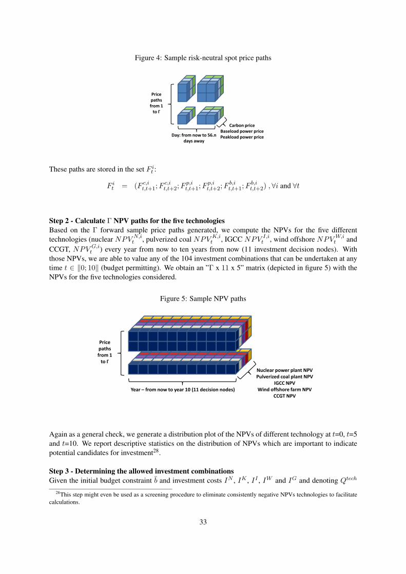
Figure 4: Sample risk-neutral spot price paths

Price

Day: from now to 56.n

days away

Price

paths

from 1

to Γ

Carbon price

Baseload power price

Peakload power price

These paths are stored in the set F it :

F it = (F c,it,t+1;F c,it,t+2;F p,it,t+1;F p,it,t+2;F b,it,t+1;F b,it,t+2) ,∀i and ∀t

Step 2 - Calculate Γ NPV paths for the five technologiesBased on the Γ forward sample price paths generated, we compute the NPVs for the five differenttechnologies (nuclear NPV N,i

t , pulverized coal NPV K,it , IGCC NPV I,i

t , wind offshore NPV W,it and

CCGT, NPV G,it ) every year from now to ten years from now (11 investment decision nodes). With

those NPVs, we are able to value any of the 104 investment combinations that can be undertaken at anytime t ∈ ‖0; 10‖ (budget permitting). We obtain an ”Γ x 11 x 5” matrix (depicted in figure 5) with theNPVs for the five technologies considered.

Figure 5: Sample NPV paths

Price

paths

from 1

to Γto Γ

Year – from now to year 10 (11 decision nodes)

Nuclear power plant NPV

Pulverized coal plant NPV

IGCC NPV

Wind offshore farm NPV

CCGT NPV

Again as a general check, we generate a distribution plot of the NPVs of different technology at t=0, t=5and t=10. We report descriptive statistics on the distribution of NPVs which are important to indicatepotential candidates for investment28.

Step 3 - Determining the allowed investment combinationsGiven the initial budget constraint b and investment costs IN , IK , II , IW and IG and denoting Qtech

28This step might even be used as a screening procedure to eliminate consistently negative NPVs technologies to facilitatecalculations.

33

the quantity of a given technology we invest in (Qtech being an integer), we recognize that at any time,the following relation must be satisfied:

xt = IN .QN + IK .QK + II .QI + IW .QW + IG.QG ≤ bt , ∀t.

We identify that the control variable can take one of the following 121 values:

xt ∈ { 0; IW ; IG; ...; IN}∈ { 0; 792; 914; ...; 5896}

And the budget can therefore take one of the following 121 values:

bt ∈ { b− IN ; ...; b− IG; b− IW ; b}∈ { 4; ...; 4996; 5108; 5900}

Step 4 - Start from the last decision node at t=10We start from t=10, the last time we are able to invest during the investment window. At this last decisionnode, the continuation value is assumed to be zero. That is to say - once the investment opportunity ismissed, there is no ability to generate cash flows from it. The value function takes the following form inwhich Si10 is a set of stochastic state variables at t=10 and on path i:

V10(b10, Si10) = max

x10

{f10(b10, x10, S

i10)},∀i.

For all the possible budget levels at b10 (121) and on all the Γ paths, we compute V10(b10, Si10). We

obtain 121 “Γ paths x 121 possible decisions” tables in which we identify the immediate reward compo-nents f10(b10, x10, S

i10). These are stored in the matrixMR10 (the matrix storing the reward functions).

Based on those tables, we determine the maximum value among f10(b10, x10, Si10) and associated in-

vestment decision for a given remaining budget level and on a given paths. These are consigned in two“Γ paths x 121 budget levels” matrices, one for the maximum value (MV10) and one for the correspond-ing optimal decision (Mx∗10).Note that the condition, x10 ≤ b10, must be satisfied. Therefore, the calculations are eased when theremaining budget actually limits the possible investment combinations (for instance when the budgetdoes not allow any additional investment, the only suitable course of action is to wait).We end up this step with the matricesMR10,MV10 andMx∗10 (check matricesMRt,MVt andMx∗tin appendix for more details) in hands.

Step 5 - Moving backward in the decision-making process (from t=9 to t=1)The value function now incorporates a continuation value and takes the following form:

V9(b9, Si9) = maxx9

{f9(b9, x9, S

i9) + e−r.EQ9 [V10(b9 − x9, S

i10)]}, ∀i and ∀ti.

In order to determine the value maximizing choice for all the remaining budget level (b9) and eachsample paths, we have to:

• compute f9(b9, x9, Si9) ∀i and ∀b9 like we did in step 4 and store the resulting 121 “Γ paths x 121

possible decisions” reward functions in matrixMR9;

• estimate e−r.EQ9 [V10(b9 − x9, Si10)] ∀i and ∀b9 using OLS regressions like we did in the prelimi-

nary stochastic case study (else that would be clairvoyance and we would be replacing a stochasticproblem by a deterministic one) and store the resulting 121 “Γ paths x 121 possible decisions”estimated continuation value functions in matrixMC9;

34

Following Cortazar et al. (2008) [45], we stress that the optimal exercise of options rather dependson expected spot prices and volatilities than on regressors being powers of all state variables (as wassuggested in the reference papers by Longstaff and Schwartz, 2001 [14] and Gamba, 2003 [46]). Theysuggest using functions on Futures, European options or bond prices that have economic meaning. Do-ing so, they find that the root mean square deviation computed is lower using this reduced form function(with various number of regressors) than using Chebyshev cross products as proposed in [14]. This alsopartially solves the OLS regression instability and performance problems present in high-dimensionalproblems as is the case here.

In particular, we consider the following OLS regression model:

e−r.EQt [Vt+1(bt − xt, Sit+1)] ≈ φt+1(bt − xt, Sit+1)

= cbt−xt0,t + cbt−xt

1,t .F c,it,t+1 + cbt−xt2,t .F p,it,t+1

+cbt−xt3,t .F b,it,t+1 + cbt−xt

4,t .F c,it,t+2

+cbt−xt5,t .F p,it,t+2 + cbt−xt

6,t .F b,it,t+2 + ebt−xti

We regress discounted continuation value (contingent on the decision taken at t) to be found inMV10

against a set of one-year and two-year forward prices for carbon, baseload power and peakload power.It should be stressed that, contrary to the preliminary stochastic case study, we do not have to estimatea single continuation value but rather up to 121. Once estimated, we store φ10(b9 − x9, S

i10) in matrix

MC9 (checkMCt in appendix for more details).

Finally, we have to:

• combine matricesMR9 andMC9 to determine V9(b9, Si9) ,∀i and ∀b9. This entails adding theMR9 andMC9 matrices and keep the maximum combined value ,∀i and ∀b9;

• store the resulting maximum combined value, i.e. V9(b9, Si9), inMV9 and related optimal deci-sions inMx∗9;

• repeat the process for t = 8 until t = 1.

Step 6 - The first decision (t=0)At t = 0, the budget variable uncertainty is resolved, we know for sure that b0=b. The value functionhence takes the following form:

V0(b, Si0) = maxx0

{f0(b, x0, S

i0) + e−r.EQ0 [V1(b− x0, S

i1)]},∀i.

In order to determine the value maximizing choice for each sample paths, we do the followings:

• We compute f0(b, x0, Si0) ∀i and store the resulting “Γ paths x 121 possible decisions” reward

functions in matrixMR0. Note that this matrix is smaller to the otherMRt matrices since onlyone budget level is possible at t=0;

• At t=0, the one-year and two-year forward prices for carbon, baseload and peakload power areknown as well since they are estimated based on current prices. This means that we cannot esti-mate e−r.EQ0 [V1(b − x0, S

i1)] using OLS regressions like we did in step 5 (as that would imply

regressing NPV combinations varying upon i against static one-year forward prices independentof i). Instead, following Longstaff and Schwartz (2001 [14]) and like we did in the illustrativecase study, we simply discount one year back V1(b − x0) ∀i to be found inMV1. The resultingapproximated continuation value is stored inMC0;

35

• We combine matricesMR0 andMC0 to determine V0(b, Si0) , ∀i. This entail adding theMR0

andMC0 matrices;

• We store the resulting value for V0(b, Si0) inMV0 and related optimal decisions inMx∗0.

Step 7 - The optimal path and implied emissionsAt this point, we have a set of eleven matricesMVt andMx∗t indicating maximum value and optimaldecisions , ∀t and ∀i.We start from t=0 and compute averages over all paths in matrixMV0 (Γ x x0 value function matrix att=0, i.e. when budget is full). Here, we look for:

V0(b) = maxx0

{1Γ

Γ∑i=1

[f0(b, x0, Si0) + φ1(b− x0, S

i1)]

}The result suggests a peculiar optimal decision (x∗0) that is expected to maximize V0 (which needs notbe identical to what is to be found inMx∗0).

We move forward in time, and solve recursively the following equation ∀t ∈ ‖1; 9‖:

Vt(b−t−1∑k=0

x∗k) = maxxt

{1Γ

Γ∑i=1

[ft(b−t−1∑k=0

x∗k, xt, Sit) + φt+1(b−

t−1∑k=0

x∗k − xt, Sit+1)]

},∀t

When at t=10, we solve the following equation (no estimated discounted continuation value):

V10(b−9∑

k=0

x∗k) = maxx10

{1Γ

Γ∑i=1

[f10(b−9∑

k=0

x∗k, x10, Si10)]

}We find a set comprised of optimal decisions (x∗0, x∗1, ..., x∗10).

Given the optimal path, we expect a given amount of locked-in CO2 emissions. That amount canbe estimated based on (1) the carbon emission factor of the technology we invest in, (2) the expectedannual production and (3) the life length of the plants.

4.2 Model results

Price path generationRecalling that the logarithm of the stochastic price processes are expressed as the sum of (1) a determin-istic linear trend and (2) a mean-reverting stochastic component, we generate deterministic log-lineartrends for the three stochastic processes based on:

hct∗ = αc + βc.t = 2.5992 + 0.0250.t (Carbon)

hpt∗ = αp + βp.t = 3.9821 + 0.0075.t (Peakload)

hbt∗ = αb + βb.t = 3.8061 + 0.0075.t (Baseload)

Figure 6 depicts the long-term trends suggested for the three processes:

We now move to the stochastic component of the sources of uncertainty:dXc

t = θc.(−λc.σc

θc − Xct ).dt+ σcdW c

t (Carbon)dXp

t = θp.(−λp.σp

θp − Xpt ).dt+ σpdW p

t (Peakload)dXb

t = θb.(−λb.σb

θb − Xbt ).dt+ σbdW b

t (Baseload)

The following parameters have been estimated jointly based on a common historical sample:

36

Figure 6: Assumed price trends over the investment lifetime

0 10 20 30 40 5010

20

30

40

50

60

70

80

90

Year

EU

R

Carbon (EUR/tCO2)Peakload power (EUR/MWh)Baseload power (EUR/MWh)

• Mean-reverting speed parameter matrix:

θc 0 00 θp 00 0 θb

=

2.4519 0 00 72.8955 00 0 53.6616

;

• Mean-reverting level parameter matrix:

−λc.σc

θc

−λp.σp

θp

−λb.σb

θb

=

0.08140.00220.0030

Note that the mean-reverting

levels are quite low since we are dealing with a detrended variable;

• Volatility parameter matrix:

σc 0 00 σp 00 0 σb

=

0.4396 0 00 3.4488 00 0 2.7786

;

• Correlation matrix:

ρc,c ρc,p ρc,bρp,c ρp,p ρp,bρb,c ρb,p ρb,b

=

1.0000 0.3599 0.29330.3599 1.0000 0.97810.2933 0.9781 1.0000

.

We generate 10,000 paths based on the stochastic processes retained and the calibration parameters.One such set of sample paths is depicted in figure 729. We compute spot, one-year and two-year forwardcontracts (see figure 8). We then compute NPV distribution (see figure 9) We run the model whichindicates that the optimal decision is to invest in six CCGT plants now which locks in 284 million tonsof carbon over their lifetime.

29We simultaneously generated paths for carbon, peakload power and baseload power mean-reverting stochastic processes.We then added the generated paths to the linear trend and took the sum to the exponential to derive three sample price paths.

37

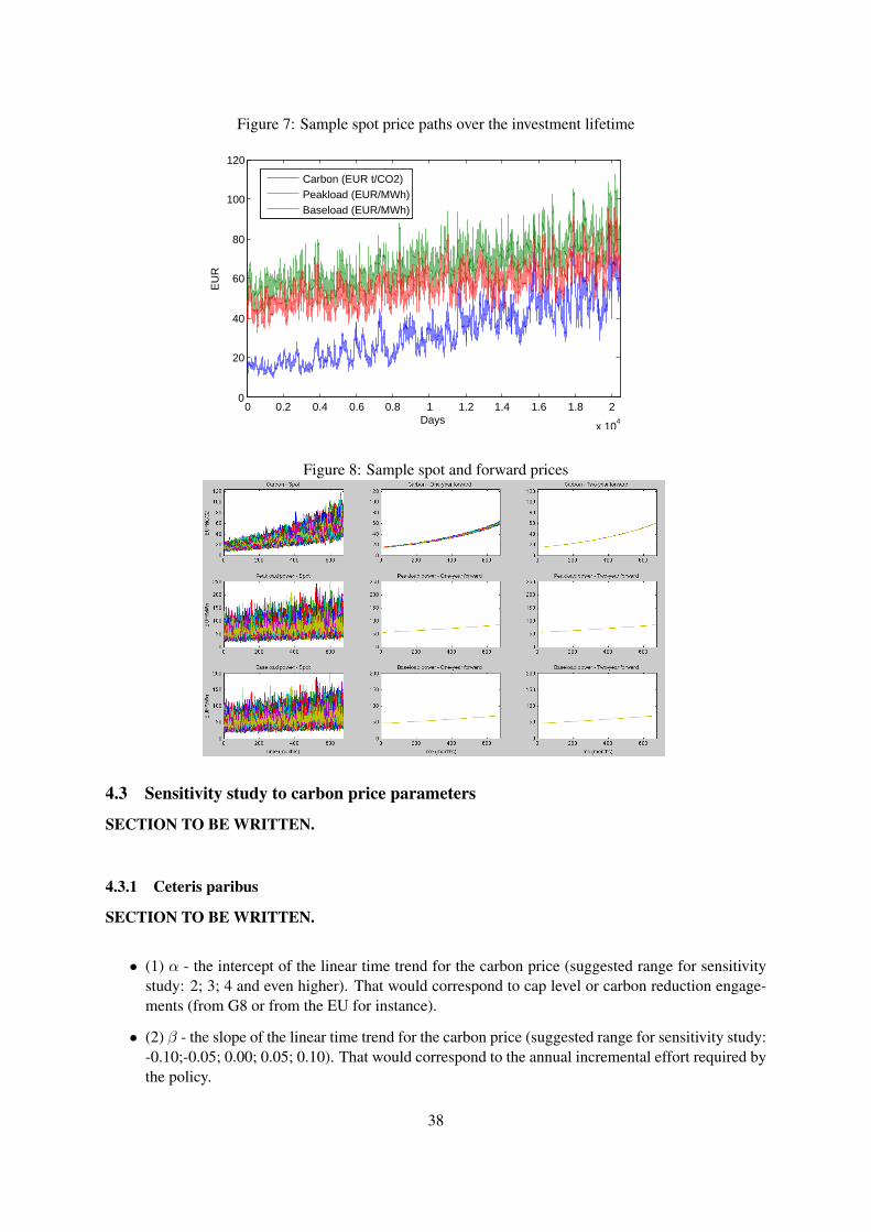
Figure 7: Sample spot price paths over the investment lifetime

0 0.2 0.4 0.6 0.8 1 1.2 1.4 1.6 1.8 2

x 104

0

20

40

60

80

100

120

Days

EU

R

Carbon (EUR t/CO2)Peakload (EUR/MWh)Baseload (EUR/MWh)

Figure 8: Sample spot and forward prices

4.3 Sensitivity study to carbon price parameters

SECTION TO BE WRITTEN.

4.3.1 Ceteris paribus

SECTION TO BE WRITTEN.

• (1) α - the intercept of the linear time trend for the carbon price (suggested range for sensitivitystudy: 2; 3; 4 and even higher). That would correspond to cap level or carbon reduction engage-ments (from G8 or from the EU for instance).

• (2) β - the slope of the linear time trend for the carbon price (suggested range for sensitivity study:-0.10;-0.05; 0.00; 0.05; 0.10). That would correspond to the annual incremental effort required bythe policy.

38

Figure 9: NPVs for technolgies at t=0, t=5 and t=10

• (3) θ - the mean-reversion speed to the linear time trend for the carbon price (suggested range forsensitivity study: 0; 2; 4; 6)

• (4) σ2 - the instantaneous volatility for the price of carbon (suggested range for sensitivity study :0.00 for the deterministic case; 0.10; 0.20; 0.30; 0.40)

Versus to following results from the dynamic programming part & emissions calculation:

• Parameter (x-axis) vs. overall profit (left y-axis) and implied emissions (right y-axis).

• Composition of the investment portfolio

• Option value for waiting

• Range (+/- 1 standard deviation around mean value) of expected prices for the expected NPV ofpower plant alternatives for the 11 decision periods.

Expectations:

• The higher α, the higher the cost of carbon, the less likely the investor will choose to invest in CF& CCGT, the lower the profit, the lower the emissions

• The higher β, the higher the cost of carbon, the less likely the investor will choose to invest in CF& CCGT, the lower the profit, the lower the emissions

• The higher θ, the less sensitive to price shocks and the further we move to the deterministic case(?) and the higher the profit, the higher the emissions

• The higher σ2, the higher the NPV range for the CCGT and the coal-fired plant, (the less likelywe will invest in them) and thus the lower the profit and the lower the emissions

4.3.2 Stylized scenarios

SECTION TO BE WRITTEN.Parameterize at best to match the trading regime

• phase I

39

• phase II

• phase III

• termination of the ETS policy

• replacement by a tax

5 Discussion

SECTION TO BE WRITTEN.Of course, in no way would price be “administrated” still, prices can be supported by means of supportpolicies to make sure that the climate policy objective remains intact. In particular, we consider:

• Cap-setting (Declining-cap within & between trading phases)

• NER & allowances fate in case of installation closure

• More flexibility mechanisms (Offset Projects & intertemporal adjustments)

• Horizon

• free-allocation vs. the impact of auctioning

• Price cap (with mean reversion speed)

• Price floor (with mean reversion speed)

• Other polices like renewables and energy efficiency (with volatility parameter)

• Help correct capital market inefficiencies (better market liquidity better informational efficiency)

• Evolution of coverage or linking to a “superior” cap-and-trade market (more constrained) (seepaper by Ellis et al.).

6 Conclusion

SECTION TO BE WRITTEN.

References

[1] F. Olsina, F. Garces, and H.-J. Haubrich. Modeling long-term dynamics of electricity markets.Energy Policy, 34:1411–1433, 2006.

[2] Y. He. Real Options in the Energy Markets. PhD thesis, University of Twente, 2007.

[3] R. Trotignon and A. Delbosc. Allowance Trading Patterns During the EU ETS Trial Period: Whatdoes the CITL Reveal? Climate Report, Mission Climat of Caisse des Depots, 2008.

[4] A.D. Ellerman and B. Buchner. Over-Allocation or Abatement? A Preliminary Analysis of the EUEmissions Trading Scheme Based on the 2006 Emissions Data. MIT Joint Program on the Scienceand Policy of Global Change Report No. 141, 2006.

40

[5] V.H. Hoffmann. EU ETS and Investment Decisions: The Case of the German Electricity Industry.European Management Journal, 25(6):464–474, 2007.

[6] A.D. Ellerman. New Entrant and Closure Provisions: How do they distort? CEEPR (MIT) WorkingPaper 06-013 WP, 2006.

[7] P.L. Joskow. Lessons Learned From Electricity Market Liberalization. The Energy Journal, Specialissue:9–42, 2008.

[8] J.-M. Chevalier and J. Percebois. Gaz et electricite : un defi pour l’Europe et pour la France.Technical report, Conseil d’Analyse Economique, 2008.

[9] M. Ventosa, A. Baillo, A. Ramos, and M. Rivier. Electricity market modeling trends. EnergyPolicy, 33:897–913, 2005.

[10] L. Trigeorgis. Real Options: Managerial Flexibility and Strategy in Resource Allocation. The MITPress, 1996.

[11] S.E. Shreve. Stochastic Calculus for Finance I: The Binomial Asset Pricing Model. SpringerFinance, 2004.

[12] S.E. Shreve. Stochastic Calculus for Finance II: Continuous-Time Models. Springer Finance, 2006.

[13] R. Bellman. Dynamic Programming. Dover Publications Inc., 1957.

[14] F.A. Longstaff and E.S. Schwartz. Valuing American options by simulation: a simple least-squaresapproach. The Review of Financial Studies, 14:113–147, 2001.

[15] A.K. Dixit and R.S. Pindyck. Investment under Uncertainty. Princeton University Press, NewJersey, 1994.

[16] M.J. Brennan and Schwartz E.S. Evaluating Natural Resource Investments. Journal of Business,58(2):135–157, 1985.

[17] R. Pindyck. Irreversible Investment, Capacity Choice, and the Value of the Firm. American Eco-nomic Review, 78(5):969–985, 1988.

[18] L.M. Abadie and J.M. Chamorro. European CO2 prices and carbon capture investments. EnergyEconomics, 30:2992–3015, 2008.

[19] M.C. Bohm, H.J. Herzog, J.E. Parsons, and R.C. Sekar. Capture-ready coal-plants - Options,technologies and economics. International Journal of Greenhouse Gas Control, 1:113–120, 2007.

[20] R.C. Sekar, J.E. Parsons, H.J. Herzog, and H.D. Jacoby. Future carbon regulations and currentinvestment in alternative coal-fired power plant technologies. Energy Policy, 35:1064–1074, 2007.

[21] R.C. Sekar. Carbon Dioxide Capture from Coal-Fired Power Plants: A Real Options Analysis.Technical report, MIT LFEE 2005-002 RP, May 2005 Report, 2005.

[22] H. Laurikka. Option value of gasification technology within an emissions trading scheme. EnergyPolicy, 2005.

[23] H. Laurikka and T. Koljonen. Emissions trading and investment decisions in the power sector - acase study in Finland. Energy Policy, 34:1063–1074, 2006.

41

[24] S. Fuss, J. Szolgayova, M. Obersteiner, and M. Gusti. Investment under market and climate policyuncertainty. Applied Energy, 85:708–721, 2008.

[25] S. Fuss, D.J.A. Johansson, J. Szolgayova, and M. Obersteiner. Impact of climate policy uncertaintyon the adoption of electricity generating technologies. Energy Policy, 37(2):733–743, 2009.

[26] W. Blyth, R. Bradley, D. Bunn, C. Clarke, T. Wilson, and M. Yang. Investment risks under climatechange policy. Energy Policy, 35:5766–5773, 2007.

[27] M. Yang and W. Blyth. Modeling Investment Risks and Uncertainties with Real Options ApproachA Working Paper for an IEA Book: Climate Policy Uncertainty and Investment Risk. Technicalreport, Paris Number LTO/2007/WP01 IEA Working Paper, 2007.

[28] E. Alberola, J. Chevallier, and B. Cheze. Price Drivers and Structural Breaks in European CarbonPrices 2005-07. Energy Policy, 36(2):787–797, 2008.

[29] M. Mansanet-Bataller, A.P. Tornero, and E.V. Mico. CO2 Prices, Energy and Weather. Universityof Valencia working paper, 2006.

[30] E. Alberola and J. Chevallier. European Carbon Prices and Banking Restrictions: Evidence fromPhase I (2005-2007). The Energy Journal, 30(3):107–136, 2009.

[31] M. Mansanet-Bataller and Pardo A. The Effects of National Allocation Plans on Carbon Markets.University of Valencia working paper, 2007.

[32] E. Benz and S. Truck. Modeling CO2 Emission Allowance Prices. SSRN Working Paper, 2006.

[33] G. Daskalakis, D. Psychoyios, and R.N. Markellos. ModelingCO2 Emission Allowance Prices andDerivatives: Evidence from the European Markets. Athens University of Economics and BusinessWorking Paper, 2007.

[34] M. Yang, W. Blyth, R. Bradley, D. Bunn, C. Clarke, and T. Wilson. Evaluating the power invest-ment options with uncertainty in climate policy. Energy Economics, 30:1933–1950, 2008.

[35] Z. Chladna. Determination of optimal rotation period under stochastic wood and carbon prices.Forest Policy and Economics, 9(8):1031–1045, 2007.

[36] J. Szolgayova, S. Fuss, and M. Obersteiner. Assessing the effects of CO2 price caps on electricityinvestments - A real option analysis. Energy Policy, 36:3974–3981, 2008.

[37] R.S. Pindyck. The Long-Run Evolution of Energy Prices. Working paper MIT, 1999.

[38] E.S. Schwartz. The Stochastic Behavior of Commodity Prices: Implications for Valuation andHedging. The Journal of Finance, 52:923–973, 1997.

[39] J.J. Lucia and E.S. Schwartz. Electricity prices and power derivatives: Evidence from the NordicPower Exchange. UC Los Angeles: Anderson Graduate School of Management, 2000.

[40] H. Geman. Commodities and Commodity Derivatives: Modeling and Pricing for Agriculturals,Metals, and Energy. John Wiley & Sons - The Wiley Finance Series, 2006.

[41] M. Mansanet-Bataller and J.H. Keppler. Causalities between CO2, Electricity, and other EnergyVariables during Phase I and Phase II of the EU ETS. Mission Climat Working Paper, 2, 2009.

[42] IEA. World Energy Outlook 2008. Technical report, OECD/IEA, 2008.

42

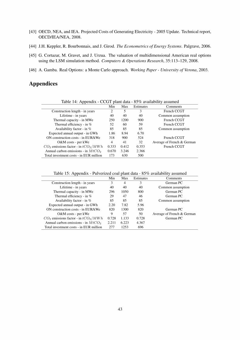
[43] OECD, NEA, and IEA. Projected Costs of Generating Electricity - 2005 Update. Technical report,OECD/IEA/NEA, 2008.

[44] J.H. Keppler, R. Bourbonnais, and J. Girod. The Econometrics of Energy Systems. Palgrave, 2006.

[45] G. Cortazar, M. Gravet, and J. Urzua. The valuation of multidimensional American real optionsusing the LSM simulation method. Computers & Operations Research, 35:113–129, 2008.

[46] A. Gamba. Real Options: a Monte Carlo approach. Working Paper - University of Verona, 2003.

Appendices

Table 14: Appendix - CCGT plant data - 85% availability assumedMin Max Estimates Comments

Construction length - in years 2 5 3 French CCGTLifetime - in years 40 40 40 Common assumption

Thermal capacity - in MWe 250 1200 900 French CCGTThermal efficiency - in % 52 60 59 French CCGTAvailability factor - in % 85 85 85 Common assumption

Expected annual output - in GWh 1.86 8.94 6.70ON construction costs - in EUR/kWe 318 900 524 French CCGT

O&M costs - per kWe 4 41 32 Average of French & GermanCO2 emissions factor - in tCO2/MWh 0.333 0.412 0.353 French CCGTAnnual carbon emissions - in MtCO2 0.670 3.246 2.366Total investment costs - in EUR million 173 630 500

Table 15: Appendix - Pulverized coal plant data - 85% availability assumedMin Max Estimates Comments

Construction length - in years 3 4 3 German PCLifetime - in years 40 40 40 Common assumption

Thermal capacity - in MWe 296 1050 800 German PCThermal efficiency - in % 29 47 46 German PCAvailability factor - in % 85 85 85 Common assumption

Expected annual output - in GWh 2.20 7.82 5.96ON construction costs - in EUR/kWe 820 1300 820 German PC

O&M costs - per kWe 9 57 50 Average of French & GermanCO2 emissions factor - in tCO2/MWh 0.728 1.133 0.728 German PCAnnual carbon emissions - in MtCO2 2.211 6.223 4.367Total investment costs - in EUR million 277 1253 696

43

Table 16: Appendix - IGCC plant data - 85% availability assumedMin Max Estimates Comments

Construction length - in years 3 4 3 German IGCCLifetime - in years 40 40 40 Common assumption

Thermal capacity - in MWe 300 450 450 German IGCCThermal efficiency - in % 43 51 46 German IGCCAvailability factor - in % 85 85 85 Common assumption

Expected annual output - in GWh 2.23 3.35 3.35ON construction costs - in EUR/kWe 1200 1692 1200 German IGCC

O&M costs - per kWe 28 81 81 German costsC02 emissions factor - in tCO2/MWh 0.656 0.780 0.656 German IGCCAnnual carbon emissions - in MtCO2 1.742 2.198 2.198Total investment costs - in EUR million 516 576 576

Table 17: Appendix - Nuclear plant data - 85% availability assumedMin Max Estimates Comments

Construction length - in years 5 9 5 ≥ 5 years include studiesLifetime - in years 40 40 40 Common assumption

Thermal capacity - in MWe 665 1600 1590 French PWRThermal efficiency - in % 30 37 36 French PWRAvailability factor - in % 85 85 85 Common assumption

Expected annual output - in GWh 4.95 11.91 11.84ON construction costs - in EUR/kWe 952 1875 1455 Average of German and French

O&M costs - per kWe 40 72 49 Average of German and FrenchTotal investment costs - in EUR million 1006 3094 2391

Table 18: Appendix - Offshore wind plant dataMin Max Estimates Comments

Construction length - in years 1 2 1Lifetime - in years 20 25 20 Most common case

Thermal capacity - in MWe 120 300 300 German offshoreEquipment availability - in % 95 95 95 Common assumption

Average load factor - in % 35 43 42 Most common caseExpected annual output - in GWh 0.36 1.13 1.20

ON construction costs - in EUR/kWe 1431 2292 1650 German offshoreO&M costs - per kWe 38 115 58 German offshore

Total investment costs - in EUR million 238 512 512

44

Tabl

e19

:App

endi

x-M

Rt

-Im

med

iate

rew

ard

com

pone

ntof

the

valu

efu

nctio

nint

f t(b−IN,0,S

1 t)

...f t

(b−IN,IN,S

1 t)

...f t

(b−IW,IG,S

1 t)

...f t

(b,0,S

1 t)

...f t

(b,IN,S

1 t)

f t(b−IN,0,S

2 t)

...f t

(b−IN,IN,S

2 t)

...f t

(b−IW,IG,S

2 t)

...f t

(b,0,S

2 t)

...f t

(b,IN,S

2 t)

...

...

...

...

...

...

...

...

...

f t(b−IN,0,S

i t)

...f t

(b−IN,IN,S

i t)

...f t

(b−IW,IG,S

i t)

...f t

(b,0,S

i t)

...f t

(b,IN,S

i t)

...

...

...

...

...

...

...

...

...

f t(b−IN,0,S

Γ t)...f t

(b−IN,IN,S

Γ t)...f t

(b−IW,IG,S

Γ t)...f t

(b,0,S

Γ t)...f t

(b,IN,S

Γ t)

=

0...−∞

...NPVG,1

t...

0...NPVN,1

t

0...−∞

...NPVG,2

t...

0...NPVN,2

t

......

...

...

...

.........

...

0...−∞

...NPVG,i

t...

0...NPVN,i

t

......

...

...

...

.........

...

0...−∞

...NPVG,Γ

t...

0...NPVN,Γ

t

45

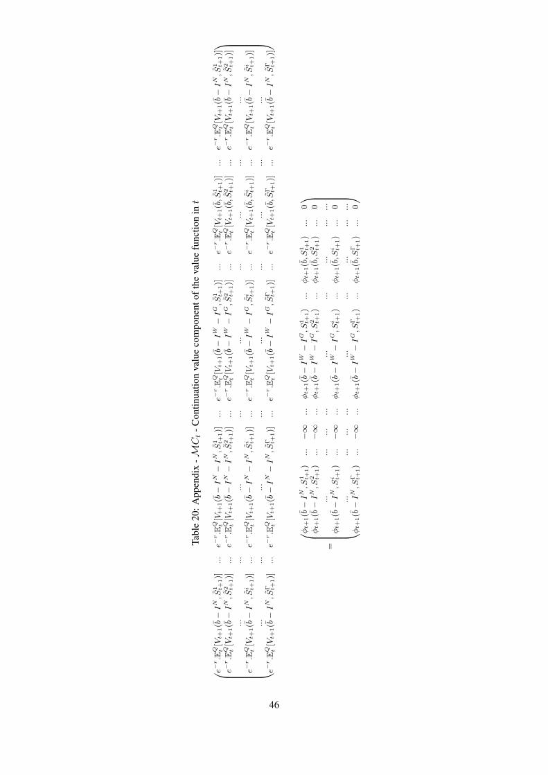
Tabl

e20

:App

endi

x-M

Ct

-Con

tinua

tion

valu

eco

mpo

nent

ofth

eva

lue

func

tion

int

0 B B B B B B @e−r.E

Q t[V

t+1(b−I

N,S

1 t+1)]

...

e−r.E

Q t[V

t+1(b−I

N−I

N,S

1 t+1)]

...

e−r.E

Q t[V

t+1(b−I

W−I

G,S

1 t+1)]

...

e−r.E

Q t[V

t+1(b,S

1 t+1)]

...

e−r.E

Q t[V

t+1(b−I

N,S

1 t+1)]

e−r.E

Q t[V

t+1(b−I

N,S

2 t+1)]

...

e−r.E

Q t[V

t+1(b−I

N−I

N,S

2 t+1)]

...

e−r.E

Q t[V

t+1(b−I

W−I

G,S

2 t+1)]

...

e−r.E

Q t[V

t+1(b,S

2 t+1)]

...

e−r.E

Q t[V

t+1(b−I

N,S

2 t+1)]

...

...

...

...

...

...

...

...

...

e−r.E

Q t[V

t+1(b−I

N,S

i t+1)]

...

e−r.E

Q t[V

t+1(b−I

N−I

N,S

i t+1)]

...

e−r.E

Q t[V

t+1(b−I

W−I

G,S

i t+1)]

...

e−r.E

Q t[V

t+1(b,S

i t+1)]

...

e−r.E

Q t[V

t+1(b−I

N,S

i t+1)]

...

...

...

...

...

...

...

...

...

e−r.E

Q t[V

t+1(b−I

N,S

Γ t+1)]

...

e−r.E

Q t[V

t+1(b−I

N−I

N,S

Γ t+1)]

...

e−r.E

Q t[V

t+1(b−I

W−I

G,S

Γ t+1)]

...

e−r.E

Q t[V

t+1(b,S

Γ t+1)]

...

e−r.E

Q t[V

t+1(b−I

N,S

Γ t+1)]

1 C C C C C C A

=

0 B B B B B B @φt+

1(b−I

N,S

1 t+1)

...−∞

...

φt+

1(b−I

W−I

G,S

1 t+1)

...

φt+

1(b,S

1 t+1)

...

0φ

t+1(b−I

N,S

2 t+1)

...−∞

...

φt+

1(b−I

W−I

G,S

2 t+1)

...

φt+

1(b,S

2 t+1)

...

0...

...

...

...

...

...

...

...

...

φt+

1(b−I

N,S

i t+1)

...−∞

...

φt+

1(b−I

W−I

G,S

i t+1)

...

φt+

1(b,S

i t+1)

...

0...

...

...

...

...

...

...

...

...

φt+

1(b−I

N,S

Γ t+1)

...−∞

...

φt+

1(b−I

W−I

G,S

Γ t+1)

...

φt+

1(b,S

Γ t+1)

...

0

1 C C C C C C A

46

Tabl

e21

:App

endi

x-M

Vt

andMx∗ t

-Val

uefu

nctio

nan

das

soci

ated

optim

alde

cisi

onint

max

xt[φt+

1(b−IN,S

1 t+1);...;−∞

]...

max

xt[φt+

1(b−IW,S

1 t+1);...;−∞

]m

axx

t[φt+

1(b,S

1 t+1);...;NPVN,1

t]

max

xt[φt+

1(b−IN,S

2 t+1);...;−∞

]...

max

xt[φt+

1(b−IW,S

2 t+1);...;−∞

]m

axx

t[φt+

1(b,S

2 t+1);...;NPVN,2

t]

...

...

...

...

max

xt[φt+

1(b−IN,S

i t+1);...;−∞

]...

max

xt[φt+

1(b−IW,S

i t+1);...;−∞

]m

axx

t[φt+

1(b,S

i t+1);...;NPVN,i

t]

...

...

...

...

max

xt[φt+

1(b−IN,S

Γ t+1);...;−∞

]...

max

xt[φt+

1(b−IW,S

Γ t+1);...;−∞

]m

axx

t[φt+

1(b,S

Γ t+1);...;NPVN,Γ

t]

argm

axx

t[φt+

1(b−IN,S

1 t+1);...;−∞

]...

argm

axx

t[φt+

1(b−IW,S

1 t+1);...;−∞

]ar

gmaxx

t[φt+

1(b,S

1 t+1);...;NPVN,1

t]

argm

axx

t[φt+

1(b−IN,S

2 t+1);...;−∞

]...

argm

axx

t[φt+

1(b−IW,S

2 t+1);...;−∞

]ar

gmaxx

t[φt+

1(b,S

2 t+1);...;NPVN,2

t]

...

...

...

...

argm

axx

t[φt+

1(b−IN,S

i t+1);...;−∞

]...

argm

axx

t[φt+

1(b−IW,S

i t+1);...;−∞

]ar

gmaxx

t[φt+

1(b,S

i t+1);...;NPVN,i

t]

...

...

...

...

argm

axx

t[φt+

1(b−IN,S

Γ t+1);...;−∞

]...

argm

axx

t[φt+

1(b−IW,S

Γ t+1);...;−∞

]ar

gmaxx

t[φt+

1(b,S

Γ t+1);...;NPVN,Γ

t]

47