Uncertainty, Innovation, and

Infrastructure Credits: Outlook for The

Low Carbon Fuel Standard through 2030 UNIVERSITY OF CALIFORNIA INSTITUTE OF TRANSPORTATION STUDIES

October 2019

James Bushnell, Professor, Department of Economics, University of California, Davis

Daniel Mazzone, Ph.D. Student, Department of Agricultural and Resource Economics,

University of California, Davis

Aaron Smith, Professor, Department Agricultural and Resource Economics, University of

California, Davis

Julie Witcover, Assistant Project Scientist, ITS, University of California, Davis

[page intentionally left blank]

Contents

Executive Summary iv

1 Introduction 1

2 Background: the California LCFS 22.1 LCFS and Infrastructure Credits . . . . . . . . . . . . . . . . . . . . . . . . 32.2 Cost Containment . . . . . . . . . . . . . . . . . . . . . . . . . . . . . . . . . 4

3 Data and Methodology 53.1 Model of BAU Demand . . . . . . . . . . . . . . . . . . . . . . . . . . . . . . 53.2 Data . . . . . . . . . . . . . . . . . . . . . . . . . . . . . . . . . . . . . . . . 73.3 Coefficient Estimates from the VEC Model . . . . . . . . . . . . . . . . . . . 93.4 BAU Demand Simulations . . . . . . . . . . . . . . . . . . . . . . . . . . . . 93.5 BAU Fuel Assumptions for Deficit Generation . . . . . . . . . . . . . . . . . 11

4 Compliance Scenarios 174.1 Deriving Implied BBD Blend Rates Required for Compliance . . . . . . . . . 174.2 Scenario Assumptions . . . . . . . . . . . . . . . . . . . . . . . . . . . . . . . 194.3 Scenario Results . . . . . . . . . . . . . . . . . . . . . . . . . . . . . . . . . . 21

5 Conclusion 24

A Appendix 28A.1 Additional Output from Simulations and the VEC Model . . . . . . . . . . . 28A.2 LCFS Credit Implementation Details . . . . . . . . . . . . . . . . . . . . . . 29A.3 Credit Generation from Infrastructure Investment . . . . . . . . . . . . . . . 31A.4 Cap on Total FCI Credits . . . . . . . . . . . . . . . . . . . . . . . . . . . . 32A.5 Additional Figures . . . . . . . . . . . . . . . . . . . . . . . . . . . . . . . . 32

i

List of Tables1 Long-Run Coefficient Estimates of the Co-Integrating Equations . . 92 BAU Assumptions for Deficit-Generating Fuels . . . . . . . . . . . . . 123 BAU EV Assumptions by Vehicle Type . . . . . . . . . . . . . . . . . 124 Summary of Compliance Scenario Assumptions . . . . . . . . . . . . 205 Short-Run Coefficient Estimates from VEC Model . . . . . . . . . . 286 Summary Statistics for Aggregate BAU Demand across Random

Samples . . . . . . . . . . . . . . . . . . . . . . . . . . . . . . . . . . . . . 297 LCFS CI Standards . . . . . . . . . . . . . . . . . . . . . . . . . . . . . . 31

ii

List of Figures1 Demand Forecasts under BAU Uncertainty . . . . . . . . . . . . . . . 112 Projected Distributions of BAU Deficits by Fuel . . . . . . . . . . . . 143 Projected Distribution of BAU LCFS Deficits . . . . . . . . . . . . . 144 LCFS Credit Generation by Pathway in 2018 . . . . . . . . . . . . . . 155 Projected LCFS Credit Generation under BAU . . . . . . . . . . . . 166 Projected Baseline Implied Blend Rate . . . . . . . . . . . . . . . . . . 227 Projected Implied Blend Rates under Compliance Scenarios . . . . 238 Price Forecasts under BAU Uncertainty . . . . . . . . . . . . . . . . . 339 Summary of the Diesel Pool under Compliance Scenarios . . . . . . 3410 Volume-Weighted CI of Ethanol from CARB ICS . . . . . . . . . . . 3511 Summary of Credit Shortages under Different Assumptions . . . . . 36

iii

Executive SummaryCalifornia’s low carbon fuel standard (LCFS) specifies that the state’s transportation fuelsupply achieve a 20% reduction in carbon intensity (CI) below 2011 levels by 2030. Reach-ing the standard will require substantive changes in the fuel mix, but the specifics and thecost of these changes are uncertain. Since the policy was extended in 2019, the price ofLCFS compliance credits has been close to its maximum allowed value, which indicatesthat fuel markets expect compliance to be expensive to achieve, if it can be achieved at all.Uncertainty surrounding compliance stems from the unknown future market penetration ofalternatives to the internal combustion engine, such as electric vehicles, as well uncertaintyabout growth in the state economy, oil prices, vehicle miles traveled, and fuel economy.

In this paper, we assess if and how California is likely to achieve the proposed 20 percentreduction in CI values by 2030, and the likely impact of infrastructure credits on this com-pliance outlook. We take an approach similar to Borenstein et al. 2019 in their paper oncap-and-trade markets. We begin by projecting a distribution of fuel and vehicle miles de-mand under BAU economic and policy uncertainty as characterized by patterns since 1987and transform those projections into a distribution of LCFS net deficits for the entire periodfrom 2019 through 2030, assuming a steady draw-down of the currently accumulated credit“bank.”

Given the stable long-run relationships between fuel markets, oil prices, vehicle miles, andgeneral economic activity, we employ a vector error correction (VEC) model to account forthe cointegration between these variables when estimating coefficients. This approach resultsin projected outcomes that become more uncertain as predictions move farther out of sampleand allows us to project a distributions of demand under business-as-usual (BAU) economicconditions. We fit our model using quarterly data from 1987-2018 and make projections foryears 2019-2030, which we refer to as the compliance period.

We then construct a variety of scenarios characterizing LCFS credit supply that considerdifferent assumptions regarding input markets, technological adoption over the complianceperiod, and the efficacy of complementary policies. By interacting our distribution of de-mand outcomes with various supply scenarios for LCFS credits, we are able to estimate theequilibrium number of LCFS credits supplied to the market for various credit-generatingsources and analyze the change in those quantities across scenarios. Given our distributionof deficits and estimates of credits under each scenario, we can assess the fuel mix in thediesel pool required to achieve annual compliance.

In our baseline scenario for credit generation, LCFS compliance would require that between60% and 80% of the diesel pool be produced from biomass. Our baseline projections have thenumber of electric vehicles reaching 1.3 million by 2030, however if the number of electric ve-hicles increases more rapidly than what is captured under BAU conditions, and reaches JerryBrown’s goal of 5 million vehicles by 2030, then LCFS compliance would require substan-tially less biomass-based diesel. Under this scenario, annual compliance could be achieved

iv

with between 10% and 25% biomass-based diesel in the diesel pool, which is commensuratewith recent levels and could be achievable with an indexed $200 credit price through 2030.

Outside of rapid ZEV penetration, compliance in 2030 with the $200 credit price may bemuch more difficult. For instance, a scenario in which CCS is widely adopted in ethanolplants would bring the median BBD blend rate down to approximately 45% BBD in 2030,rather than 60%. However, a 45% blend rate in 2030 under this scenario still results in nearlya 125% increase from current levels. Additionally, if increasing BBD production calls for anincreasing amount of higher-CI feedstocks, the implied blend rate required for compliancecould increase above the baseline. If the volume-weighted average CI rating of BBD were toincrease only to 50, the median draw requires nearly 100% of diesel to be biomass-based.

New mechanisms to allow firms to generate credits by building electric vehicle chargingstations or hydrogen fueling stations have minor implications for overall compliance. Thismechanism represents a major departure from the original design of the LCFS as it does notdirectly subsidize the consumption of a low carbon fuel. Rather, the credits subsidize a fixedcost of providing network infrastructure that may encourage adoption of EVs, the technologywhich may in turn use a low carbon fuel. In the same way, however, the infrastructure creditcan reduce the very effect that LCFS critics have focused on as the central flaw in theregulations design: the encouragement of low, but still non-zero carbon fuel. Nonetheless,because the total quantity of infrastructure credits is restricted to be relatively small, theireffect on potential compliance scenarios is small.

v

1 IntroductionState and local policy makers in the U.S. and beyond are looking to Low Carbon Fuel Stan-dards (LCFS) as a policy instrument for reducing GHG emissions in the transportationsector. California implemented its LCFS in 2011, setting a target of a ten percent reductionin carbon intensity (CI) values for transport fuels used in the state by 2030 from 2011 levels,as part of its climate policy. The target has since been updated to a 20 percent reductionbelow 2011 levels by 2030. Oregon fully implemented its LCFS, the Clean Fuels Program(CFP), in 2016, seeking to reduce CI values of Oregon transportation fuels by ten percentfrom 2015 to 2025.1 2 Washington State failed in several legislative attempts to pass a LCFSthat proposed a ten percent reduction over a ten-year period, most recently in 2019.3 Alsoin Washington State, Puget Sound Air Quality Agency is considering a regional clean fuelstandard to contribute to its 2030 GHG emissions goals.4 Other jurisdictions with, devel-oping, or considering an LCFS-like program include British Columbia (in effect since 2011),Canada and Brazil (under development), and Colorado (initial feasibility analysis). 5

While the LCFS regulation is now moving forward, its history is not without controversy.There have been legal challenges linked to the way it differentiates fuels originating in dif-ferent locations. There have also been extensive debates about the life cycle calculationsused to establish the carbon intensities of different fuels used for compliance, particularlyaspects linked to the indirect land use effects caused by bio-fuels. More recently, opponentshave pointed to increasing costs of compliance and raised concerns about both the efficiencyof the regulation and its potential impact on fuel prices. Such concerns contributed to therejection of the LCFS mechanism in some states.

Partly in response to concerns over compliance costs, and partly in an effort to spur moreinnovation, new dimensions have continued to be added to the LCFS. In California, regula-tors have allowed the expansion of “book-and-claim,” an accounting mechanism that allowscertain specialized fuels, particularly bio-methane sourced from dairy digesters to be physi-cally consumed in one state but still allowed to generate LCFS credits in another. In anotherdeparture from the original design, the LCFS will also now award credits for investment ininfrastructure related to EV charging facilities and hydrogen fueling station. This decouplingof credit generation from fuel consumed within the state could affect both the long run creditprice and its transmission through to various types of fuels. However, such effects will ariseonly if sufficient infrastructure credits are generated to alter the long-run marginal optionsfor compliance.

In this paper, we assess if and how California is likely to achieve the proposed 20 percent1See https://www.oregon.gov/deq/aq/programs/Pages/Clean-Fuels.aspx for more information on

the Oregon CFP.2See, also, https://escholarship.org/uc/item/0ct4m7gs.3See https://washingtonstatewire.com/whats-next-for-a-low-carbon-fuel-standard/.4See https://www.pscleanair.org/528/Clean-Fuel-Standard/.5For information on Colorado, see https://ngtnews.com/colorado-looks-into-establishing-

carbon-fuel-standard.

1

reduction in CI values by 2030, and the likely impact of infrastructure credits on this com-pliance outlook. We follow a general methodology similar to that used in Borenstein et al.2019 for the California cap-and-trade program. We apply time-series econometric methodsto account for uncertainty in demand under business-as-usual (BAU) as indicated by his-torical data on a range of key variables. We begin by projecting a distribution of demandfor fuel and vehicle miles under BAU economic and policy uncertainty, which we define ascontinuation of the trends and correlations since 1987. We then transform those projectionsinto a distribution of LCFS net deficits for the entire period from 2019 through 2030, as-suming a steady drawdown of the currently accumulated credit “bank.” The distribution ofnet deficits illustrates a range of possibilities of demand for LCFS credits based on historicaltrends. Next, we generate LCFS credit supply scenarios that consider a variety of assump-tions about inputs, technology, and the efficacy of complementary policies. By interactingprojections of demand and various supply scenarios for LCFS credits, we can characterize theequilibrium number of credits generated under varying policy conditions and, furthermore,illustrate the changes in the fuel mix that would be necessary to achieve compliance.

For sources of credits generation not yet prevalent in the policy, we use ARB figures basedon the modeling it used in its scoping plan. These sources include the potential role of a newcategory for credit generation, ZEV infrastructure capacity credits.6 Credit supply scenariosalso cover certain state goals, showing sensitivity of results to, for example, meeting theGovernor’s goals for battery electric vehicles in the light duty sector by 2030. State poli-cies impacting the demand side such as vehicle efficiency standards and target reductionsin vehicle miles traveled, are not explicitly modeled, although the modeled uncertainty inBAU takes account of past trends in these variables and allows for considerable variability.Targeted scenario modeling of demand side policies and additional supply side policies is apossible area for future research.

The remainder of this paper is structured as follows. Section 2 describes the background ofthe California LCFS, discussing the history of the policy, recent trends, and the economicmechanisms through which CI standards influence markets. In section 3, we describe ourdata and econometric model used to forecast BAU demand for LCFS credits and discussthe projected outcomes. In section 4, we characterize a variety of scenarios regarding LCFScredit supply and assess annual compliance in each. Finally, in section 5, we conclued bydiscussing the implications of our analysis and highlight opportunities for future research.

2 Background: the California LCFSThe California Low Carbon Fuel Standard was initially implemented in 2011, amended in2013, re-adopted in 2015, and extended in 2019 to set targets through 2030. The LCFS setsa carbon intensity (CI) standard percentage reduction from the petroleum-based referencefuel that decreases each year. Implementation involves classifying all fuel volumes into afuel pool defined by the reference fuel used or displaced and setting a nominal CI standard

6ARB credit generation assumptions from the scoping plan modeling include that a variety of state targetswill be met, and an LCFS credit price of approximately $125/MTCO2e.

2

for each fuel pool. The reference fuels are diesel, E10 gasoline, and, from 2019 forward, jetfuel. The LCFS falls within a general regulatory framework known as intensity standards.It regulates the carbon intensity (e.g., gCO2e per megajoule) of transportation fuels, ratherthan the total amount of CO2 released through fuels.

As with all intensity standard mechanisms, the LCFS implicitly subsidizes the sales of fuelsthat are cleaner – that is, lower in carbon intensity – than the standard, and pays for thesubsidy through charges imposed on fuel that is ‘dirtier’ than the standard (CI rating abovethe standard). Sales of individual fuels rated at a CI below the standard generate credits,and fuels rated at a CI above the standard generate deficits, in amounts proportionate tovolumes. The LCFS requires annual compliance by regulated entities; all incurred deficitsmust be met by credits generated by production of low-carbon fuels or purchased from acredit market. The units of LCFS credits are dollars per metric ton of CO2e. LCFS creditscan be banked without limit, allowing overcompliance under less stringent standards to helpcover increased obligations as the standard grows more stringent, and they are fungible –meaning credits generated in any fuel pool are treated equivalently.

One of the attractions of policies like the LCFS to the policy community is that these sub-sidies and charges work to partially offset each other and dilute the pass-through of theimplied carbon cost to retail fuel prices. This ‘feature’ of the LCFS has also been criticizedby environmental economists, who note that the dilution of the carbon cost works to encour-age more fuel consumption than would arise under alternative instruments such as a carbontax.7 In an extreme case, the subsidy of ‘cleaner’ fuel could spur consumption growth to thepoint where the quantity of fuel that is consumed overwhelms the reduction in the carbonintensity of the fuel and carbon emissions can increase. This extreme case is unlikely as itwould require extremely price-elastic fuel demand. However, the overall point that, relativeto other regulations, the LCFS can encourage consumption of fuels has continued to raiseconcerns in some circles.

CARB set annual standards for the CI of fuels in both the diesel and gasoline pools. Theseannual mandates are shown in the appendix in table 7. LCFS credits are awarded to fuelswith a reported CI rating below the standard and deficits to those above the standard. Thenumber of credits per unit of fuel depends on the CI rating of that fuel. The LCFS is energy-based and thus the number of credits per unit of fuel also depends on factors regarding theenergy output of the fuel.8

2.1 LCFS and Infrastructure CreditsEarly policy development and academic research on the LCFS focused on its characteristicas an intensity standard targeting the marginal costs of fuels. As described above, per unitcosts of cleaner fuels would be reduced through the subsidy effect and the costs of dirtierfuels would reflect the cost of acquiring credits. Recent revisions to the LCFS program have

7See Holland, Hughes, and Knittel 2009.8See Holland, Hughes, and Knittel 2009 for more information regarding energy-based LCFS relative to

other types of LCFS.

3

increased the role of alternative forms of compliance, in particular, the ability of firms togenerate credits through the installation of infrastructure, rather than the production of fuel.

Fueling infrastructure credits are limited to zero tailpipe emission vehicles (ZEVs), hydrogenfuel cell vehicles and battery electric vehicles. LCFS infrastructure credits can be gener-ated based on potential fuel flow from unused operational capacity for publicly accessiblehydrogen fueling stations and DC fast chargers. ZEV infrastructure credits are capped at5% of the prior quarter’s deficit generation – 2.5% for hydrogen fueling and 2.5% for DCfast charging equipment. Applications for ZEV infrastructure credits are open through 2025,and are valid for 15 years in the case of hydrogen infrastructure, and 5 years in the case ofDC fast charging infrastructure.

On one level, the addition of infrastructure credits represents a major departure from theoriginal design of the LCFS as it does not directly subsidize the consumption of a low carbonfuel. Rather, the credits subsidize a fixed cost of providing network infrastructure that mayencourage adoption of EVs, the technology which may in turn use a low carbon fuel. In thesame way, however, the infrastructure credit can reduce the very effect that LCFS criticshave focused on as the central flaw in the regulations design: the encouragement of low,but still non-zero carbon fuel. While infrastructure credits may spur vehicle adoption, theireffect on expanding driving miles would be second order.

At the same time, if the amount of infrastructure credits awarded through the program weresignificant enough to ease compliance, these credits can have the effect of lowering the overallLCFS credit price, and therefore reduce even the diluted carbon price effect on end-use fuelprices. The magnitude of any price-suppression effect would depend upon both the quantityof infrastructure credits and the slope of the LCFS compliance cost curve.

2.2 Cost ContainmentInitially, there were no formal limits on how high LCFS credit prices could rise, althoughlegal challenges to the regulation effectively delayed implementation, freezing the standardfrom 2013 through 2015, and effectively limited demand for credits and their pass-throughto fuel prices. However, as the lawsuits were resolved in favor of continued implementationof the LCFS and the standard declined steadily in the last several years (with the exceptionof a court-ruled hiatus for the diesel pool standard in 2017-2018, which resumed its trajec-tory in 2019), credit prices have risen steadily and raised increasing concerns about the costof the regulation.9 In its 2015 re-adoption rule, the ARB introduced the credit clearancemarket, which is a cost-containment mechanism that would in theory limit price increasesunder some scenarios.

Entities in need of LCFS credits for purposes of immediate compliance can purchase creditsin the credit clearance market at a price no higher than the prescribed maximum of $200 per

9Historical LCFS credit prices can be accessed via the Data Dashboard at the ARB website: https://ww3.arb.ca.gov/fuels/lcfs/dashboard/dashboard.htm.

4

ton in 2016 and adjusted for inflation thereafter (currently $216 per ton). If these entitiesare unable to purchase sufficient credits in this market to reach compliance, then they maycarry over their deficits to future periods. Carryover deficits grow by 5% per year, mean-ing that firms pay an ‘interest’ penalty for deferring compliance. However, firms that holdcredits are not required to sell in the credit clearance market, and they would not do so ifthey believed that they be able to sell their credits at a higher price in the future. Thus,the credit clearance market provides only a soft cap. However, ARB is currently proposingto impose a hard price cap of $200 per ton in 2016 dollars for LCFS credit transactions. Tohelp facilitate compliance under this cap, it proposes a mechanism to ‘borrow credits’ fromfuture residential electric vehicle charging. Under this mechanism, obligated entities coulduse credits expected to be generated in 2026-2030 to meet unmet annual deficit obligationsin 2020 – 2025.

These cost-containment mechanisms are suited for dealing with a transient disruption inclean fuel supply or some other cause of a short-term supply-demand imbalance of LCFScredits. Because of the requirement that borrowed credits be restored with interest, it will notbe effective at containing costs in an environment of chronic, long-term credit supply demandimbalance. The future prospects of the regulation are therefore linked to the potential supplyand demand balance through the next 11 years of the program. A circumstance wherecompliance is only feasible through high cost fuels or sharp reductions in fuel consumptionwould push credit prices above the maximum credit price for the credit clearance market.One objective of this paper is to assess the potential likelihood of such an outcome. In2019, ARB is proposing amendments that would backstop this cost containment mechanism,enforcing additional borrowing of future credit generation from residential electricity chargingfor electric vehicles at the maximum credit price, with a rolling payback schedule enforcedon utilities that will borrow the credits, up to a cumulative total of 10 million borrowedcredits.

3 Data and MethodologyThis section outlines data and methods used to project business-as-usual (BAU) for LCFScredit and deficit generation to 2030. In this paper we use the term business-as-usual (BAU)frequently, and take it to mean, regarding LCFS credit demand, the continuation of historicaltrends through the compliance period. For LCFS credit supply, BAU refers to a continuationof current alternative fuel mix trends to 2030. Therefore, the uncertainty in the projectionsstems from the estimation of BAU demand, which against an assumed steady state of supply,yields a distribution of net deficits accumulate over the period 2019 to 2030, on which webase subsequent analysis.

3.1 Model of BAU DemandWe are interested forecasting demand for fuel and vehicle miles under BAU economic condi-tions. Demand for fuel and vehicle miles are highly dependent on other economic variables.Demand for both fuel and vehicle miles will be influenced by general economic activity and

5

oil prices. In a booming economy, consumers travel more and purchase more fuel. Our aimis to fit an econometric model that characterizes past trends in key credit demand variablessuch as fuel consumption and key input prices for the gasoline and diesel fuel “pools,” namelyoil price and soybean prices, vehicle miles traveled, and an indicator of the state economy.10

The estimates from that model are then used to simulate relationships moving forward toproject potential credit demand.

Let Xt = (X1t, X2t . . . , X6t)′ denote the vector composed of the six variables included in ourmodel used to characterize the BAU environment, where t is at the quarterly level. The sixcomponents of Xt are

X1t = California Reformulated Gasoline ConsumptionX2t = California Diesel Fuel ConsumptionX3t = U.S. Soybean PricesX4t = California Vehicle Miles Traveled (VMT)X5t = Brent Oil PriceX6t = California Gross State Product (GSP)

Define Yit = ln(Xit) for i = 1, . . . 6 and Yt = (Y1t, Y2t, . . . Y6t)′. We fit a cointegrated vectorerror correction (VEC) model to Yit. Cointegration allows the variables to have one or morestable long-run relationships. We specify three cointegration relationships:

Y1t = β10 + β11Y4t + β12Y5t + β13Y6t + z1t (1)Y2t = β20 + β21Y4t + β22Y5t + β23Y6t + z2t (2)Y3t = β30 + β32Y5t + z3t (3)

The first equation represents the demand for gasoline and the second represents the demandfor diesel. The third equation implies that soybean and crude oil prices are tied together inthe long run. We impose zero coefficients on VMT and GSP in the third equation becausewe have no rationale for these California variables to be tied to the soybean price.11 The zitterms represent the deviations from the cointegration relationship, also known as the errorcorrection terms.

The VEC model to estimate the interrelationships among the six credit demand variables is:

∆Yt = αzt−1 +p−1∑j=1

Γj∆Yt−j +4∑

k=1wksk + εt (4)

10The list includes soybean prices to capture trends in commodity prices. It may also improve the model’sability to project trends in use of biomass-based diesel within the diesel pool.

11The purpose of this third equation is to model the marginal cost of producing biomass-based diesel,which can then be used to model LCFS credit price under the assumption that biomass-based diesel is themarginal compliance fuel. We do not conduct that analysis in this paper; we defer it to future research.

6

where ∆ is the first-difference operator, sk are seasonal indicators for the quarter of the year,p = 4 so that three quarterly lags of Yt are included in the model, and εt is a vector ofidiosyncratic disturbances. The 6× 3 matrix α represents how the six variables respond todeviations from the cointegration relationship. Putting equations 1-3 together with equation4, we can write the model as:

∆Yt = αβ0 + αβ′Yt−1 +p−1∑j=1

Γj∆Yt−j +4∑

k=1wksk + εt (5)

where

β =

1 0 00 1 00 0 1−β11 −β21 0−β12 −β22 −β32−β13 −β23 0

and β0 = (−β10,−β20,−β30)′.

3.2 DataWe use data available from 1987 to 2018 for the six dependent variables to fit the VEC model.Because our data are measured at the quarterly level, we have a total of 124 observationsfor each variable.12 California GSP was collected from the Bureau of Economic Analysis(BEA).13 The oil prices used in our model are Europe Brent spot prices FOB collectedfrom the Energy Information Administration (EIA) at the monthly level and aggregated toquarterly averages.14 We chose to use Brent oil prices rather than West Texas Intermediate(WTI) prices because Brent prices are more relevant to California markets. Historical vehi-cle miles traveled (VMT) on California highways are reported by the California Departmentof Transportation, CalTrans, at the monthly level.15 On-highway VMT data are reportedin the aggregate, and not divided into gasoline and diesel vehicles.16 Our model also re-

12All variables are measured at the quarterly level except CA GSP. The Bureau of Economic Analysis(BEA) reports quarterly data only since the year 2003. Therefore, we use annual data for CA GSP, whichis available for the entire sample 1987-2018.

13Available at https://apps.bea.gov/regional/downloadzip.cfm14Historical Brent oil prices can be found at https://www.eia.gov/dnav/pet/hist/LeafHandler.ashx?

n=PET&s=RBRTE&f=M.15Available at http://www.dot.ca.gov/trafficops/census/mvmt.html16We divide highway VMT by 0.56 to scale it up to an approximate total VMT. We use a factor of

0.56 because, when we compare on-highway VMT from Caltrans to total VMT from EMFAC, we find thaton-highway VMT make up 56% of total VMT in CA on average. This re-scaling has no effect on thecoefficient estimates or BAU projections from the VEC model described in the previous subsection becauseit is effectively just a change in units for one of the predictor variables. We re-scale the variable because laterin our analysis when we estimate EV charging loads, we need to estimate VMT coming from EVs, which

7

quires soybean prices, which we collect from the Agricultural Marketing Service (AMS) atthe United States Department of Agriculture (USDA).17 We aggregate monthly spot pricesin Central Illinois to quarterly averages to be used in the model.

The main variables of interest in our model are gasoline and diesel consumption and VMTin California as we need to forecast BAU fuel demand in order to construct a distribution ofLCFS deficits. We collect monthly prime supplier sales volumes for California reformulatedgasoline (CaRFG) from the EIA.18 This measure captures all finished gasoline that is con-sumed in California, including imports to the state. We assume all gasoline is consumed inthe transportation sector.

Measuring diesel fuel consumption is more nuanced. The EIA reports monthly sales volumesfor refiners at each step in the supply chain. We aggregate wholesale and retail sales volumesfor No.2 distillate to construct a measure of consumption of No.2 distillate. According todata from the EIA, 99 percent of No.2 distillate is used for diesel fuel in California. There-fore we calculate sales volumes of CARB diesel, which is ultra-low sulfur diesel (ULSD)sold in California, as 99 percent of No.2 distillate sales. The diesel pool, however, com-prises biomass-based diesel (BBD), which includes biodiesel and renewable diesel, as well aspetroleum diesel. BBD demand was negligible prior to 2011, but has been increasing in theyears since. Therefore, we construct the measure for diesel fuel consumption as the sum ofBBD and ULSD. The EIA does not report sales of BBD, so we use volumes reported byCARB in the LCFS quarterly summary, since the years of substantial BBD demand occurin that time period.19 We aggregate monthly CARB diesel sales from the EIA to quarterlytotals and add quarterly volumes of BBD from CARB.

The LCFS regulates fuel used in the California transportation sector. Therefore, to accu-rately estimate the number of deficits generated from CARB diesel using our data, we needto measure the amount of diesel fuel consumed in California that is allocated to the trans-portation sector. Since 1992, approximately 70% of distillate consumed in California hasbeen used on-highway in the transportation sector.20 We therefore make the assumption, inaccordance with our definition of BAU, that 70% of all CARB diesel will be consumed in thetransportation sector in each year over the 2019-2030 compliance period. We are unaware ofinformation that would lead us to believe a divergence from this long term could occur andwe don’t consider altering this assumption in this study. Importantly, scaling diesel by aconstant has no effect on the coefficient estimates in the VEC model that we use to generate

means we need total VMT rather than on-highway VMT.17The soybean prices used in this study can be accessed by creating a custom report in the Market

News Portal at https://www.ams.usda.gov/market-news/custom-reports and querying Central Illinoissoybean under grains.

18The EIA classifies a prime supplier as ”a firm that produces, imports, or transports selected petroleumproducts across State boundaries and local marketing areas, and sells the product to local distributors, localretailers, or end users.”

19The LCFS quarterly summary can be accessed at https://ww3.arb.ca.gov/fuels/lcfs/lrtqsummaries.htm

20Historical distillate sales in California by end-use sector can be accessed at https://www.eia.gov/dnav/pet/pet_cons_821usea_dcu_nus_a.htm

8

our BAU simulations.

3.3 Coefficient Estimates from the VEC ModelThe long-run coefficient estimates from the VEC cointegration model appear in table 1.Collectively, the coefficient estimates presented here make up the β matrix, therefore char-acterizing the long-run, cointegrating relationships between the variables in our model using1987-2018 data. The three columns in table 1 correspond to the three cointegrating equa-tions specified in equations 1, 2, and 3 and the rows to their long-run relationships withGSP, VMT, and the oil price.

Table 1: Long-Run Coefficient Estimates of the Co-Integrating Equations

ln(CaRFG) ln(Diesel) ln(SB Price)ln(VMT) -0.360*** -0.539 0

(0.0740) (0.521) (0)ln(Oil Price) 0.0318 -0.359*** -0.250

(0.0188) (0.0875) (0.247)ln(GSP) 0.164*** 1.024*** 0

(0.0449) (0.316) (0)Constant 21.93 9.153 3.491

Observations 123 123 123Standard errors in parentheses

*** p<0.01, ** p<0.05

In the first two equations (columns) of table 1, gasoline and diesel demand in California,the coefficients on the oil price capture the price responsiveness of demand for each fuel.The elasticity for diesel is larger in magnitude and has the expected sign. The elasticity forgasoline, on the other hand, is positive but qualitatively small, and statistically insignificantat the 5% level. This may reflect fact that gasoline demand is very inelastic. The coefficientson GSP reflect the income effect. Gasoline and diesel fuel are normal goods and thus shouldbe expected to be positively correlated with income in the state. The coefficient on VMTcaptures fuel economy improvements as more VMT per gallon implies fewer gallons. Becausethe VMT measure is not reported by vehicle type, implied fuel efficiency gains in each ofthe two fuel pools are not discernible. In the next section, we use the long-run coefficientestimates from table 1, along with the short-run estimates located in the appendix in table5, along with random shocks to project a range of forecasts for gasoline, diesel, and vehiclemiles demand out to 2030.

3.4 BAU Demand SimulationsWe use the coefficient estimates from the VEC model to predict the distribution for eachvariable through the compliance period, 2019-2030. Specifically, we simulate 1000 poten-

9

tial values for each variable in each quarter during the compliance period. To this end,we assume that the potential shocks εt that may occur in the compliance period have thesame distribution as the shocks during our estimation sample period, 1987-2018. Using thisassumption, we simulate potential future shocks by sampling randomly with replacementfrom the the 1987-2018 shocks. For each random draw, we use the VEC model to generatea hypothetical path for the six variables. We repeat this exercise 1000 times to give us adistribution of potential paths.

Specifically, for each simulation k = 1, 2, ..., 1000, we generate hypothetical future values forthe six variables by iterating on the following equation for t from 2019 through 2030:

Ykt = Yk,t−1 + αβ0 + αβ′Yk,t−1 +p−1∑j=1

Γj∆Yk,t−j +4∑

k=1wksk + ε∗kt (6)

where ε∗kt is the kth random draw from the estimation-sample residuals. For observations inthe sample period, we use Ykt = Yt and ε∗kt = εt, which means that the simulation replicatesobserved data until the end of 2018 and then simulates a hypothetical path after 2018. Weback out the projected levels of each variable for each simulation k as Xikt = exp{Yikt} fori = 1, 2, . . . , 6.

The hypothetical paths for blended gasoline, diesel, and VMT, simulated using equation6, are described in figure 1 with the median draw from each year (solid line) and a 90%pointwise confidence interval (dashed lines).21 In addition to those variables, we calculatethe fuel economy of gasoline vehicles that is implied under BAU conditions. To do so, wemultiply each VMT projection by the percent estimated in ARB’s EMFAC model to comefrom gasoline-powered vehicles (approximately 90%).22 Then we can express the averagefuel economy, measured in miles per gallon (MPG), for gasoline vehicles by dividing gasolineVMT in each draw by the number of gallons of CaRFG. The implied fuel economy shown infigure 1d highlights the range of efficiency gains considered in our simulations over the com-pliance period. This implied gasoline vehicle economy, derived from EMFAC percentagescombined with our projections, is a fleet-wide average for gasoline powered vehicles only,and does not explicitly build in the recent California vehicle efficiency agreement with majorautomakers to reduce GHG emissions per mile for model years 2022 through 2026.23

For each variable in our VEC model, the level of future uncertainty grows as we move furtherinto the future. In figure 1a, 90% of the draws from our sample fall between 14 and 17 billiongallons of CaRFG being consumed in 2030 - a 12 percent increase and 13 percent decrease,

21Plots of GSP, oil prices, and soybean prices can be found in the appendix.22Using data from ARB’s EMFAC model, we find that gasoline-powered vehicles make up approximately

90% of California VMT and is projected to decline slowly over the next decade due to EV penetration. Weuse this projected percentage in each year to find VMT attributable to gasoline vehicles for each draw of oursimulations.

23See https://www.reuters.com/article/us-autos-emissions/california-four-automakers-defy-trump-agree-to-tighten-emissions-rules-idUSKCN1UK1OD.

10

respectively, from current levels. By similar calculations, the 90% confidence interval forconsumption of diesel falls between a 10 percent reduction and 75 percent increase from cur-rent levels by 2030. The range of possibilities for diesel consumption is shown in figure 1b.Lastly, VMT increases above current levels in 90% of the draws as shown in figure 1c. VMThas been far less volatile than gasoline and diesel consumption in California and thereforewe see a tighter range of uncertainty around future VMT projections.

(a) CaRFG (b) Diesel

(c) VMT (d) Implied MPG of Gasoline

Figure 1: Demand Forecasts under BAU Uncertainty

3.5 BAU Fuel Assumptions for Deficit GenerationEach gallon of CaRFG contains reformulated blendstock for oxygenate blending (CARBOB)and ethanol. Due to the “blend wall” for ethanol, CaRFG, as well as all reformulated gaso-line in the U.S., is often referred to as E10. The average gallon of ethanol earns LCFS creditssince the volume-weighted CI rating of ethanol used in the program falls below the standard.Therefore each gallon of CaRFG consumed in California will generate both LCFS deficits

11

and credits. We calculate total CARBOB consumption as 90 percent of CaRFG, with theremaining 10 percent being ethanol. Therefore, the BAU projection assumes that the E10blend wall persists through 2030. Pursuant to our definition of BAU, currently observedBBD blend rate in the liquid diesel pool persists through 2030 as well. That is, we assumethat 20 percent of liquid diesel fuel used in the transportation sector is BBD. The BAUprojection extends the status quo assumption to fuel CI ratings over the compliance period.In the case of the biofuels, recent average volume-weighted CI ratings reported to the LCFSare used. These assumptions are summarized in table 2.

Table 2: BAU Assumptions for Deficit-Generating Fuels

Gasoline PoolShare of Total Fuel CI

CARBOB 0.90 100.82Ethanol 0.10 65

Diesel PoolShare of Total Fuel CI

CARB Diesel 0.8 100.45Biodiesel 0.05 30Renewable Diesel 0.15 34

The one area where BAU assumptions differ from the status quo is electric vehicles. Wehave to make an assumption regarding the penetration of electric vehicles to forecast creditgeneration from electricity as well as to forecast the level of fossil fuel displacement. EVpenetration is difficult to predict and its trends have been evolving. For this reason, we useEMFAC projections of the share of all vehicles that are light-duty electric and heavy-dutyelectric.24 EMFAC projects 1.3 million EVs on California roads by 2030. Table 3 shows howEMFAC projections translate into parameters that measure EV penetration in Californianow and in 2030; we follow the EMFAC rate of penetration in our BAU. Table 3 also showsour BAU assumptions regarding the CI rating of electricity. We use the current grid averageCI rating and EERs reported by CARB. Policies in place to reduce the CI rating of the gridthrough increased use of renewables or accelerate penetration of EVs are not implementedin the BAU, but considered in scenarios on the BAU and sensitivity analyses on results.

Table 3: BAU EV Assumptions by Vehicle Type

2019 Share of Pop.: 2030 Share of Pop.:EV Type CI EER EER-Adj. CI EVs All Vehicles EVs All VehiclesLDV 81.49 3.5 23.28 0.95 0.007 0.7 0.025HDV 81.49 5 16.30 0.05 0.001 0.3 0.01

In addition to the assumptions in table 3, we assume in the BAU that future EVs will replacethe average internal combustion engine vehicle (ICEV) on the light duty side but be driven

24See https://ww3.arb.ca.gov/msei/downloads/emfac2017_users_guide_final.pdf

12

30 percent fewer miles, again taking the BAU stance of extending current conditions to 2030(Davis 2019). We have no information on how VMT for the heavy-duty sector may changewith increasing EV penetration. While vehicles deployed may be well used, as currently thecase, fleets and loads may also shift in unexpected ways. For this exercise, for simplicity,we apply the “30 percent fewer miles” assumption also to heavy-duty EVs and assess thedisplaced petroleum fuel all from the gasoline pool25. With these assumptions, we can projecta quantity of kwHs of electricity that will be charged and project the resulting number ofLCFS credits associated with the demand simulations. Since EVs are assumed to replaceaverage fuel economy ICEVS, gasoline demand declines according to the share of EVs in thevehicle pool. Specifically, we calculate the number of kwHs for light duty EVs according tothe following equation:

kwHt = St ∗ (0.7 ∗X4t) ∗ 0.32 (7)

where St is the share of EVs to all vehicles in year t, X4t is vehicle mile demand from the VECmodel, and the 0.32 scale factor translates miles into kwHs.26 Then, credits from electricitycan be calculated by plugging in the number of kwHs into equation 18.

Using the parameters from table 2 and 3, we translate the forecasts of fuel demand, afteraccounting for gasoline displacement from EVs, into forecasts of the deficit/credit balanceover the compliance period subject to BAU conditions. Using the predictions of CaRFG anddiesel demand, we calculate CARBOB and CARB diesel deficits in each state of the worldrepresented by our simulations.27 The distributions of deficits from each fuel are plotted infigure 2. Figure 2a shows a distribution of CARBOB deficits centered around 290 MMTon average, or approximately 26 MMT per year. For context, the average is approximately150 percent larger than the 10.3 MMT generated in 2018. The increase in deficits reflectsthe BAU demand projections as well as the increasing stringency of the standard to 2030:a gallon of fuel of a given CI rating generates more deficits in later years because a higherpercentage CI reduction is required to meet the standard.

The total demand for LCFS credits plotted in figure 3 is the sum of CARBOB and CARBdiesel deficits, less the bank of system-wide credits accumulated since the beginning of theLCFS, reflecting CI rating reductions beyond required annual levels; the bank currently holdsapproximately 8.5 million metric tons (MMT) of credits. This distribution characterizes thenumber of LCFS credits that would need to be supplied to the market to cover aggregatedeficits expected to be generated under BAU conditions for the period 2019-2030. Notethat our approach is high-level, examining aggregate net deficits for the compliance period,and abstracting away from annual compliance decisions and situations that could impact

25These simplifying assumptions do not appreciably impact results given the low assumed HDV penetrationlevels during the period. At higher penetration levels, assumptions about and implementation of HDV fueldisplacement could be important to volumes of biofuels required for compliance, and the treatment usedhere for simplicity would no longer suffice.

26The AFDC reports this: https://afdc.energy.gov/vehicles/electric_emissions_sources.html27See equation 18 in the Appendix for more details.

13

(a) CARBOB (b) CARB Diesel

Figure 2: Projected Distributions of BAU Deficits by Fuel

year-to-year credit availability.

Figure 3: Projected Distribution of BAU LCFS Deficits

14

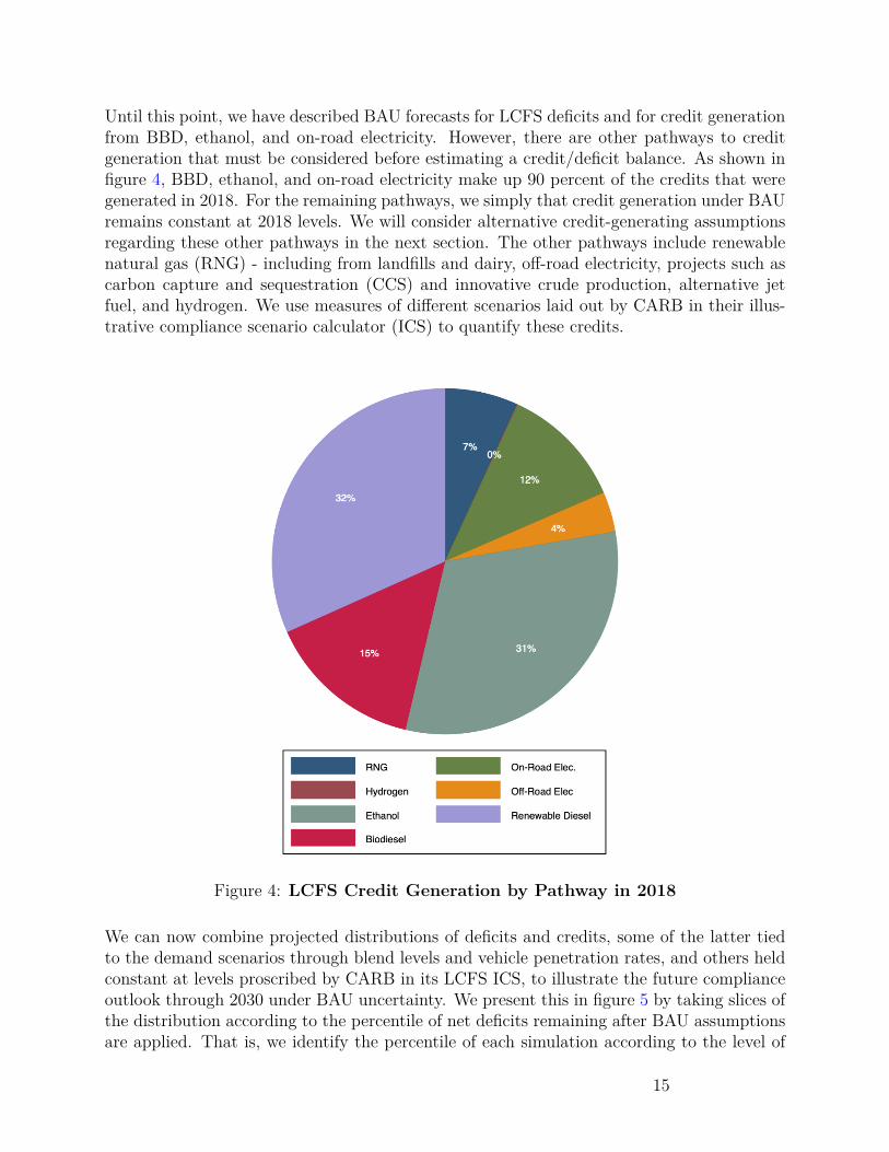
Until this point, we have described BAU forecasts for LCFS deficits and for credit generationfrom BBD, ethanol, and on-road electricity. However, there are other pathways to creditgeneration that must be considered before estimating a credit/deficit balance. As shown infigure 4, BBD, ethanol, and on-road electricity make up 90 percent of the credits that weregenerated in 2018. For the remaining pathways, we simply that credit generation under BAUremains constant at 2018 levels. We will consider alternative credit-generating assumptionsregarding these other pathways in the next section. The other pathways include renewablenatural gas (RNG) - including from landfills and dairy, off-road electricity, projects such ascarbon capture and sequestration (CCS) and innovative crude production, alternative jetfuel, and hydrogen. We use measures of different scenarios laid out by CARB in their illus-trative compliance scenario calculator (ICS) to quantify these credits.

Figure 4: LCFS Credit Generation by Pathway in 2018

We can now combine projected distributions of deficits and credits, some of the latter tiedto the demand scenarios through blend levels and vehicle penetration rates, and others heldconstant at levels proscribed by CARB in its LCFS ICS, to illustrate the future complianceoutlook through 2030 under BAU uncertainty. We present this in figure 5 by taking slices ofthe distribution according to the percentile of net deficits remaining after BAU assumptionsare applied. That is, we identify the percentile of each simulation according to the level of

15

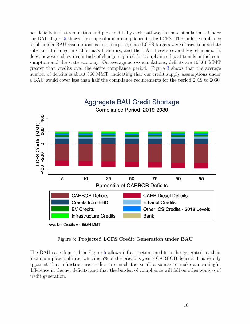
net deficits in that simulation and plot credits by each pathway in those simulations. Underthe BAU, figure 5 shows the scope of under-compliance in the LCFS. The under-complianceresult under BAU assumptions is not a surprise, since LCFS targets were chosen to mandatesubstantial change in California’s fuels mix, and the BAU freezes several key elements. Itdoes, however, show magnitude of change required for compliance if past trends in fuel con-sumption and the state economy. On average across simulations, deficits are 163.61 MMTgreater than credits over the entire compliance period. Figure 3 shows that the averagenumber of deficits is about 360 MMT, indicating that our credit supply assumptions undera BAU would cover less than half the compliance requirements for the period 2019 to 2030.

Figure 5: Projected LCFS Credit Generation under BAU

The BAU case depicted in Figure 5 allows infrastructure credits to be generated at theirmaximum potential rate, which is 5% of the previous year’s CARBOB deficits. It is readilyapparent that infrastructure credits are much too small a source to make a meaningfuldifference in the net deficits, and that the burden of compliance will fall on other sources ofcredit generation.

16

4 Compliance ScenariosOur projection of deficits under BAU uncertainty provides a range of possibilities of demandfor LCFS credits. Next, we present compliance scenarios in which we overlay a range ofpossibilities for LCFS credit supply. We begin with a baseline scenario and then consideradjustments to each of the baseline assumptions.

Throughout, we make the assumption that biomass-based diesel will be the marginal fuelfor compliance under the LCFS. This is the most likely case given past trends, and due topolicy and capacity constraints inherent with other regulated pathways. Of current creditgenerators, the constraint from the ethanol blendwall is notable. Blends of ethanol up to E85require a specialized vehicle not being prioritized for sales. E15, while allowable nationally,must go through an additional approval process for use within state.28 Massive growth innewer technologies such as hydrogen, natural gas, or electric vehicles would require thosetechnologies to be lower cost than the already mature renewable diesel. This may be possible,or additional credit generating opportunities may be opened up by regulatory amendmentsas in the past (e.g., recent expansion to book-and-claim for RNG use upstream in refineries),but these situations are too unknown or uncertain to be included here.

In the previous section, we presented a distribution of credit shortages assuming that BAUtrends continue on both the demand and supply side. In this section we relax assumptionson the supply side and answer the question of how much BBD would be necessary to reachannual compliance under the LCFS. We take this approach to evaluating the difficulty ofcompliance because BBD is the marginal fuel for compliance. Therefore, we consider dif-ferent assumptions regarding credit generation and assume the resulting net deficits mustbe satisfied by BBD credits. We assume a smooth drawdown of the existing credit bankgoing into the study period and require annual compliance through use of additional fuels,neither of which is imposed by the regulation. Our analysis is meant to illustrate difficultyof compliance.

4.1 Deriving Implied BBD Blend Rates Required for ComplianceDeficits from CARBOB and diesel demand in each draw arise directly from the VEC model,as described above, and require no additional assumptions. Net deficits from CARBOB arecalculated as

NDCt ≡ DC

t − elecont − etht − infrat − othert − bankt (8)

where NDCt is equal to CARBOB deficits net of credits from on-road electricity, ethanol, in-

frastructure, the other sources from the ICS, and the bank. We assume the bank is allocatedequally across the 11-year compliance period. Infrastructure credits are assumed to bind atthe constraint; they are assumed to equal 5% of the prior quarter’s CARBOB deficits in each

28See https://www.agri-pulse.com/articles/12295-market-demand-for-e15-looks-to-be-modest.

17

quarter in each draw. The constraint is described in detail in section A.4 of the appendix.

The number of credits generated per gallon of ULSD and BBD for each year will dependon the reported CI of both fuels, as well as the diesel CI standard in each year. The CIstandards for both gasoline and diesel are reported in the appendix in table 7. The next steprequires additional notation. Define Dt as demand for diesel fuel in year t, Bt as BBD, Ut asULSD, NDC

t as net deficits from CARBOB, φBt as the number of credits earned per gallonof BBD, and φUt as the number of credits per gallon of ULSD. BBD is the sum of biodieseland renewable diesel; Bt ≡ BDt +RDt, where BDt is biodiesel and RDt is renewable diesel.The reported CI for CARB diesel is currently 100.45 and is expected to remain there until2030. Therefore φUt is known for all t. Contrastingly, the future of reported CIs of BBD isuncertain and will depend on a few different factors.

The CI ratings of both biodiesel and renewable diesel are highly dependent on the feedstock.Waste oils and animal fats are rated as having relatively low life-cycle emissions and thusare rated with a very low CI. Used cooking oil (UCO) and tallow currently generate thelion’s share of LCFS credits from BBD. However, it is plausible that UCO and tallow willexperience supply shortages due to capacity constraints under a rapidly growing demand forBBD over the next decade. Soybean oil, on the other hand, is much more scalable and couldmore easily meet high demand for BBD. Soybean oil, however, has a considerably higher CIrating due to its impact on land use emissions, which would make lower credit generationfrom a given volume of BBD. Given the uncertainty around the CI ratings of BBD, we con-sider different assumptions around their time paths.

Conditional on the CI ratings used for BBD, the number of credits per gallon of BBD, φBtwill be known and then we can solve the following system of two equations for the twounknowns, Bt and Ut for t = 2019, 2020, . . . , 2030.

Dt = Bt + Ut (9)NDC

t = φBt Bt + φUt Ut (10)

Using simple algebra, the quantities of Ut and Bt that satisfy the system of equations are:

U∗t =Dt − NDC

t

φBt

1− φUt

φBt

(11)

B∗t =Dt − NDC

t

φUt

1− φBt

φUt

(12)

Using equations 11 and 12, we can calculate the diesel pool blend rate that would be required

18

for compliance under each of our scenarios accordingly:

BR∗t ≡B∗t

U∗t +B∗t(13)

4.2 Scenario AssumptionsCertain elements of credit supply are tied to demand, whereas we assume others are inde-pendent of demand. We calculate the factors that depend on demand from output of theVEC model and the simulations. Ethanol volumes in each simulation, for example, are equalto 10 percent of gasoline demand so we calculate the volume of ethanol for each draw of thesimulations.

For the factors that are separate from demand we run our simulation using different policyand supply scenarios to understand their impact. To characterize the relative influence ofdifferent assumptions, we evaluate each scenario against a baseline. In the baseline scenario,we assume all CI ratings remain at 2018 levels, infrastructure credits are maximized, and theother credit generating catogories achieve the minimum values in the ICS. In table 4 we sum-marize each scenario and its assumptions, relative to the BAU assumptions in the previoussection and the baseline compliance scenario. In all scenarios, we assume that infrastructurecredits are at the maximum allowable level of 5% of the previous year’s CARBOB deficits.

The other credits we use from ARB’s ICS are independent of our model of demand for LCFScredits. They are developed within the ARB modeling system, based on demand scenarios,and policy and credit pricing assumptions (of a steady level around $125) out to 203029.To illustrate the magnitude in which these sources could affect BBD demand and LCFScompliance, we consider a scenario in which the maximum of each source across scenarios isrealized. Specifically, we take the maximum number of credits across the ICS scenarios ineach year for each pathway. This set of assumptions is A1 in table 4. This characterizes ascenario with a higher credit profile for renewable natural gas and projects.

We consider a scenario in which the number of EVs rises sharply over the compliance period.In 2018, California Governor Jerry Brown announced a $2.5 billion plan with the objectiveof getting 1.5 million zero-emission vehicles (ZEV) on California roads by 2025 and 5 millionby 2030.30 This trajectory would be a stark deviation from any historical trends and wouldnot be captured in our model of BAU fuel demand. Therefore, we consider a scenario inwhich 1.5 million EVs are on the road by 2025 and 5 million by 2030 at a constant rate. Werefer to this set of assumptions as A2 in table 4.

The CI rating of ethanol is also independent of demand. The future path of the CI value29We do not explicitly model credit price, but extrapolate from trends visible under historical credit

pricing.30See https://www.washingtonpost.com/national/california-gov-jerry-brown-unveils-25-

billion-plan-to-boost-electric-vehicles/2018/01/27/deed8cd8-039f-11e8-8acf-ad2991367d9d_story.html.

19

Table 4: Summary of Compliance Scenario Assumptions

Label ComplianceScenario

EVPopulation

EthanolCI

BBDCI

ICSCredits

BAU - 1.3M by 2030 65 32 2018 levelsA0 Baseline 1.3M by 2030 65 32 MinA1 Max ICS Credits 1.3M by 2030 65 32 Max

A2 Jerry Brown’sZEV Goal

1.5M by 2025;5M by 2030 65 32 Min

A3 Dec. Ethanol CI 1.3M by 2030 65 → 40 32 MinA4 Inc. BBD CI 1.3M by 2030 65 32 → 50 Min

for ethanol will depend on technology development and adoption. CARB, in the ICS, as-sume a path for starch, sugar, and cellulosic ethanol in which the volume-weighted averageCI rating of ethanol falls to 40 by 2030, a 38.5 percent reduction from the current level.31

This CI reduction stems from assumed industry-wide adoption of CCS as well as increasesin volumes of sugar ethanol in the near future and cellulosic ethanol toward the end of thedecade. Therefore, we consider a scenario in which the ICS CI projections are realized. Werefer to these set of assumptions as A3 in table 4.

In addition to ethanol, the future path of the CI value for BBD is uncertain, as previouslymentioned. We consider a scenario in which the volume-weighted average CI rating of BBDrises from its current level of approximately 32 to 50, a rating more commensurate withsoybean oil feedstocks. This represents a future in which soybean oil makes up the majorityof the BBD feedstock pool, to provide a bound on uncertainty in this parameter. This isassumption A4 in table 4.

Beyond the four scenarios presented in this paper, we considered adjusting other assumptionsin our analysis; none had a qualitatively different impact on the implied BBD blend rateresults. For example, a scenario where a cleaner electricity grid is achieved, resulting in agrid-average CI reduction for electricity, as would occur as renewables’ penetration continues,did not substantially impact results. Even with a zero CI rating for electricity over thecompliance period had only small impacts on the implied BBD blend rate required forcompliance. CI rating improvements for electricity are diluted relative to those for otherfuels due to the relative efficiency of electricity, measured by the EER. Similarly, additionalpenetration of biogas with a substantial negative CI rating due to methane capture, into thenatural gas used as a transport fuel did not have a large impact. Other potential scenariosthat may be salient to LCFS compliance, such as expanded use of book-and-claim for low-CIrated electricity and biogas elsewhere in the production process, are left to future research.

31The specific path for the ethanol CI rating assumed in the ICS can be found in figure 10 in the appendix.

20

4.3 Scenario ResultsHere we present the output from four different compliance scenarios and discuss their differ-ences from the baseline. In each scenario, we calculate the volume of CARB diesel, BBD,and the resulting implied blend rate of BBD in the diesel pool using equations 11, 12, and13, respectively. Figure 6 shows the implied blend rate resulting from the baseline scenarioand figure 7 shows the blend rate under the alternative scenarios. For brevity, we presentonly the implied blend rates here, but the volumes of BBD and CARB diesel resulting fromeach scenario can be found in the appendix figure 9.

Because we force annual compliance, the annual quantities of BBD and ULSD, and the im-plied BBD blend rates, in the figures are conditional on compliance in the previous year.Due to the decreasing CI standards, shown in table 7, this characteristic has important im-plications for interpretation of our results; all else equal, BBD production shifted from oneyear to the next will earn fewer credits since the CI rating will be closer in magnitude tothe standard, and the yet-to-be displaced diesel would earn more deficits as its CI ratingfalls farther above the standard. Therefore, if the path of any of the blend rates picturedin this section weren’t met in early years, the implied blend rate required for compliance inlater years would rise disproportionately more. In that sense, all of our scenarios depict alower-bound of BBD implied blend rates needed for overall compliance over the eleven-yearspan. The annual compliance constraint also abstracts away from real-world optimizationdecisions on credit banking and deficit carryover. We did not model a proposed provisionfor credit borrowing.

Figure 6 shows that, under the baseline scenario, the median outcome calls for an increasein the BBD blend rate from the 2018 level of 17% to 70% in 2030. In nominal terms, givenour demand projections, this outcome implies ramping up BBD consumption in the state to3.5 billion gallons in 2030, nearly a 300% increase from current levels, and a reduction inCARB diesel consumption to 1.7 billion gallons in 2030, more than a 50% reduction belowcurrent levels.

Our median baseline scenario results in a BBD blend rate in diesel fuel similar to the highdemand/low EV scenario in CARB’s ICS, which is the highest among their four scenarios.Shown by the dashed lines in figure 6, 90% of the blend rates from our simulations fall be-tween 60 and 80 percent BBD in 2030. Next, we alter our baseline assumptions one by oneand observe how the implied blend rate required for annual compliance changes.

Figure 7a shows that allowing for the largest number of credits from the other sources in theICS (see discussion above for context on ARB’s modeling assumptions in the ICS) in eachyear would result in a blend rate of 50% BBD, rather than 60, for the median draw fromthe simulations. Thus, the range of possibilities for the other pathways makes only a smalldifference to the BBD required to meet the standard. Thus, although pathways such as re-newable natural gas, off-road electricity, CCS and innovative crude production at refineries,alternative jet fuel, and hydrogen receive significant attention in LCFS policy discussions,their influence on compliance scenarios is relatively minor, as considered in ARB scoping

21

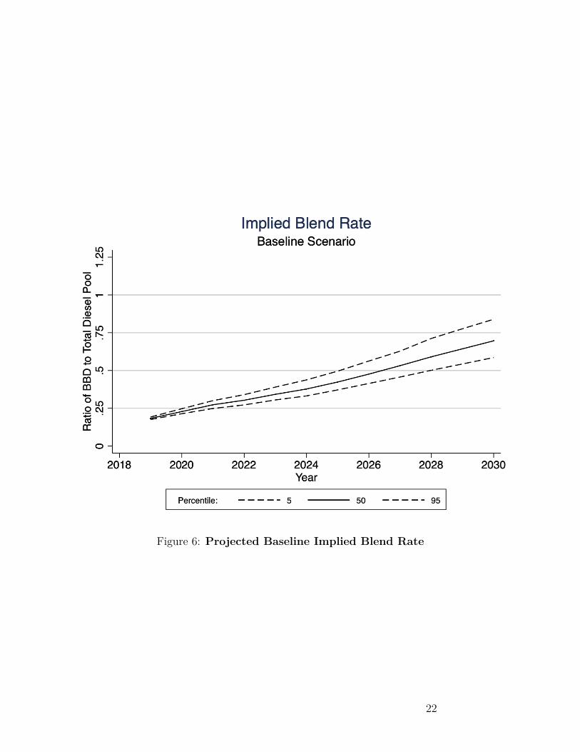
Figure 6: Projected Baseline Implied Blend Rate

22

(a) A1. ICS Maximum Credits (b) A2. Jerry Brown’s Goal Achieved

(c) A3. Declining Ethanol CI (d) A4. Increasing BBD CI

Figure 7: Projected Implied Blend Rates under Compliance Scenarios

23

plan modeling.

In contrast, rapid EV growth has the potential to reduce the blend rate below 25% in 2030,as shown in figure 7b. This is by far the largest reduction from the baseline in any of ourscenarios, and it is the only scenario that projects compliance without dramatic changes inthe diesel pool. The median required BBD blend in 2030 is approximately 20%, and the90% confidence interval ranges from 12% to 27%.

Scenarios A3 and A4 move the difficulty of compliance in opposite directions. A decliningethanol CI rating, due to CCS and increases in cellulosic and sugar ethanol volumes, wouldreduce the pressure on BBD production. Figure 7c shows that the median draw would havea BBD blend rate of approximately 45%, compared to 60% in the baseline. The lower boundof the 90% confidence interval is 37%, which is double the current BBD blend rate.

On the other hand, if the CI rating for BBD were to increase due to insufficient availabilityof low-CI feedstocks such as used cooking oil and a corresponding shift towards soybeanoil, then the median BBD blend rate would need to rise to 90 percent in 2030 to achievecompliance, as shown in figure 7d. The upper bound of the 90% confidence interval exceedsone, which means that compliance would not be achieved even if every on-road diesel gallonwas 100% BBD. We have no reason to believe that one of A3 and A4 is more likely than theother. These two scenarios can be viewed as a widening of the baseline confidence intervalto include possibilities that are both more optimistic and more pessimistic for compliance.32

5 ConclusionThe California LCFS sets out to achieve a 20% reduction in carbon intensity (CI) in thestate’s transportation sector below 2011 levels by 2030. Reaching the standard will requiredramatic changes in the fuel mix in California, but the relative push needed from individualfuel sources is uncertain and will depend upon both demand and supply factors over thenext decade. One of the most critical aspects of understanding compliance is future demandfor fuel; the demand for LCFS credits will be explicitly tied to consumption of gasoline anddiesel fuel in the state. Therefore, we estimate a distribution of fuel demand under business-as-usual (BAU) uncertainty, i.e. the continuation of historic trends, in order to estimate adistribution of demand for LCFS credits over the 2019-2030 compliance period. We estimatethat gasoline and diesel will generate between 320 and 410 million metric tons (MMT) ofdeficits in the LCFS program over the eleven-year period. In 2018, a total of 11.2 MMTcredits were generated. For context, if the lower-bound of the distribution of credit demandwere realized, the market would need to supply 29 MMT credits per year on average, nearlya 170% increase from 2018 levels. State policies such as those targeting VMT and efficiencystandards, represent a separate source of demand uncertainty, although the BAU uncertainty

32In the current LCFS structure, BBD credit generation beyond the on-road diesel pool is allowed foralternative jet fuel, of which a type derived in a similar manner to on-road RD is commercially available.We do not explicitly model use of RD in on-road or jet applications, or other credit generation possibilitiesin the program that could drive the implied BBD blend rate lower.

24

embraces a wide range of potential trajectories for each measure.

On the credit supply side, uncertainty surrounding compliance stems from the unknown fu-ture market penetration of alternatives to the internal combustion engine, such as electricvehicles, as well as uncertainty around adoption of technologies such as carbon capture andsequestration (CCS). We assume the marginal compliance fuel in the LCFS is biomass-baseddiesel (BBD) and we show that BBD’s role in compliance could vary widely depending on,in addition to BAU demand conditions, the pace of EV adoption in the state. The adoptionof CCS and other CI-reducing technologies and the market for feedstocks used to produceBBD also could have significant effects.

In our baseline scenario for credit generation, LCFS compliance would require that between60% and 80% of the diesel pool be produced from biomass. Our baseline projections have thenumber of electric vehicles reaching 1.3 million by 2030, however if the number of electric ve-hicles increases more rapidly than what is captured under BAU conditions, and reaches JerryBrown’s goal of 5 million vehicles by 2030, then LCFS compliance would require substan-tially less biomass-based diesel. Under this scenario, annual compliance could be achievedwith between 10% and 25% biomass-based diesel in the diesel pool, which is commensuratewith recent levels and could be achievable with an indexed $200 credit price through 2030.

Outside of rapid ZEV penetration, hitting 2030 targets with the $200 credit price may bemuch more difficult. For instance, a scenario in which CCS is widely adopted in ethanolplants would bring the median BBD blend rate down to approximately 45% BBD in 2030,rather than 60%. However, a 45% blend rate in 2030 under this scenario still results in nearlya 125% increase from current levels. Additionally, if increasing BBD production calls for anincreasing amount of higher-CI feedstocks, the implied blend rate required for compliancecould increase above the baseline. If the volume-weighted average CI rating of BBD were toincrease only to 50, the median draw requires nearly 100% of diesel to be biomass-based.

Since 2016, ARB has expanded credit generation opportunities in the program, and someopportunities are relatively new. The pathways as modeled in the ICS make little apprecia-ble qualitative difference to results. This study provides a range of the magnitude of creditgeneration, under uncertainty, that such expanded opportunities would need to provide toappreciably change the compliance outlook from one more to one less reliant on cost con-tainment mechanisms.

New mechanisms to allow firms to generate credits by building electric vehicle chargingstations or hydrogen fueling stations have minor implications for overall compliance. Thismechanism represents a major departure from the original design of the LCFS as it does notdirectly subsidize the consumption of a low carbon fuel. Rather, the credits subsidize a fixedcost of providing network infrastructure that may encourage adoption of EVs, the technol-ogy which may in turn use a low carbon fuel. In the same way, however, the infrastructurecredits can reduce the very effect that LCFS critics have focused on as the central flaw in theregulations design: the encouragement of low, but still non-zero carbon fuel. Nonetheless,because the total quantity of infrastructure credits is restricted to be relatively small, their

25

effect on potential compliance scenarios is small.

26

ReferencesBorenstein, Severin et al. (2019). “Expecting the unexpected: Emissions uncertainty and

environmental market design”. In: American Economic Review Forthcoming.Davis, Lucas W (2019). “How much are electric vehicles driven?” In: Applied Economics

Letters, pp. 1–6.Holland, Stephen P., Jonathan E. Hughes, and Christopher R. Knittel (2009). “Greenhouse

Gas Reductions under Low Carbon Fuel Standards?” In: American Economic Journal:Economic Policy 1.1, pp. 106–146. issn: 1945774X. doi: 10.1257/pol.1.1.106.

27

A AppendixThis appendix contains figures, tables, and equations that are referenced in the text andmay be relevant to the reader.

A.1 Additional Output from Simulations and the VEC ModelThe estimates of the β and Γ matricies from the VEC model in equation 5 appear in table5.

Table 5: Short-Run Coefficient Estimates from VEC Model

∆Y1t ∆Y2t ∆Y3t ∆Y4t ∆Y5t ∆Y6tPanel A: Estimates of α Matrix

Y1,t−1 -0.0510 0.298 -0.00667 -0.451*** 2.411** -0.0763(0.0432) (0.323) (0.660) (0.0736) (0.990) (0.102)

Y2,t−1 -0.0144* -0.0810 0.351*** -0.0287** -0.397** -0.0380*(0.00835) (0.0625) (0.128) (0.0142) (0.192) (0.0198)

Y3,t−1 0.000911 0.0604* -0.161** -0.0251*** 0.220** 0.00565(0.00417) (0.0312) (0.0637) (0.00710) (0.0956) (0.00989)

Panel B: Estimates of Γ Matrix∆Y1,t−1 -0.275** -0.0759 -0.129 0.600*** 0.589 0.260

(0.108) (0.807) (1.648) (0.184) (2.474) (0.256)∆Y1,t−2 -0.0544 0.0761 0.400 0.572*** 2.242 0.313

(0.104) (0.775) (1.583) (0.177) (2.377) (0.246)∆Y1,t−3 -0.0796 -0.286 -1.608 0.508*** -1.984 -0.365

(0.0989) (0.740) (1.512) (0.169) (2.269) (0.235)∆Y2,t−1 3.73e-05 -0.727*** -0.212 0.0279 0.00140 0.0619*

(0.0146) (0.109) (0.223) (0.0249) (0.335) (0.0347)∆Y2,t−2 0.00945 -0.440*** -0.00404 0.0434 0.155 0.0465

(0.0160) (0.119) (0.244) (0.0272) (0.366) (0.0379)∆Y2,t−3 0.00852 -0.115 -0.225 0.0307 0.184 0.0193

(0.0132) (0.0990) (0.202) (0.0226) (0.303) (0.0314)∆Y3,t−1 -0.00969 -0.0905* 0.433*** 0.00728 0.0205 0.00417

(0.00691) (0.0517) (0.106) (0.0118) (0.159) (0.0164)∆Y3,t−2 -0.0171** -0.00126 -0.0565 0.0178 0.166 -0.0261

(0.00712) (0.0533) (0.109) (0.0121) (0.163) (0.0169)∆Y3,t−3 0.00353 0.0540 -0.0261 0.0187 -0.280* 0.00215

(0.00709) (0.0531) (0.108) (0.0121) (0.163) (0.0168)∆Y4,t−1 0.0454 0.339 0.533 -0.374*** 0.756 -0.0233

(0.0482) (0.361) (0.737) (0.0822) (1.106) (0.114)∆Y4,t−2 0.0492 0.741** -0.639 -0.430*** 0.263 -0.124

(0.0490) (0.366) (0.748) (0.0835) (1.123) (0.116)Continued on next page...

28

Table 5 – Continued from previous page∆Y1t ∆Y2t ∆Y3t ∆Y4t ∆Y5t ∆Y6t

∆Y4,t−3 0.0350 0.116 -0.854 -0.451*** -0.259 -0.0532(0.0483) (0.362) (0.738) (0.0824) (1.108) (0.115)

∆Y5,t−1 -0.00528 0.0308 -0.0714 -0.0117 0.227** 0.0236**(0.00439) (0.0328) (0.0670) (0.00748) (0.101) (0.0104)

∆Y5,t−2 0.0136*** 0.0475 -0.0745 -0.00220 -0.0388 0.0111(0.00445) (0.0333) (0.0680) (0.00759) (0.102) (0.0106)

∆Y5,t−3 5.75e-06 0.00899 -0.0414 -0.00743 0.174 -0.00728(0.00461) (0.0345) (0.0705) (0.00786) (0.106) (0.0109)

∆Y6,t−1 -0.0764* -0.162 0.653 -0.0152 -1.834* -0.114(0.0460) (0.345) (0.704) (0.0785) (1.056) (0.109)

∆Y6,t−2 -0.00840 -0.214 -0.238 0.0405 0.263 0.0147(0.0463) (0.346) (0.707) (0.0789) (1.062) (0.110)

∆Y6,t−3 0.0281 0.258 1.375** -0.00511 0.859 -0.0175(0.0434) (0.325) (0.664) (0.0740) (0.996) (0.103)

Constant -0.0152** -0.0985** -0.0270 -0.0525*** 0.00160 -0.0105(0.00620) (0.0464) (0.0947) (0.0106) (0.142) (0.0147)

Observations 123 123 123 123 123 123Standard errors in parentheses

*** p<0.01, ** p<0.05, * p<0.1

In table 6 we summarize the distribution of demand forecasts coming out of the simulationsover the compliance period. Total VMT, diesel, and gasoline demand forecasts are aggregatedover the 2019-2030 time-frame for each draw.

Table 6: Summary Statistics for Aggregate BAU Demand across Random Samples

Variables N Mean SD Min MaxVMT (Billion mi.) 1000 14310.25 141.664 13734.2 14763.78Diesel (Billion gal.) 1000 152.666 6.403 133.186 173.577CaRFG (Billion gal.) 1000 669.158 6.889 649.944 696.943

A.2 LCFS Credit Implementation DetailsIn this subsection of the appendix, we provide details regarding how credits are generatedunder the LCFS. To illustrate how quantities of fuel translate into credits or deficits, weadopt the notation of the LCFS regulation and define the following terms.

• I is the set of credit-generating fuels.

• XD ∈{gasoline, diesel} represents the fuel being displaced.

• EERXDi is the dimensionless Energy Economy Ratio (EER) of fuel i relative to gasoline

or diesel. The EER is fuel and vehicle specific.

29

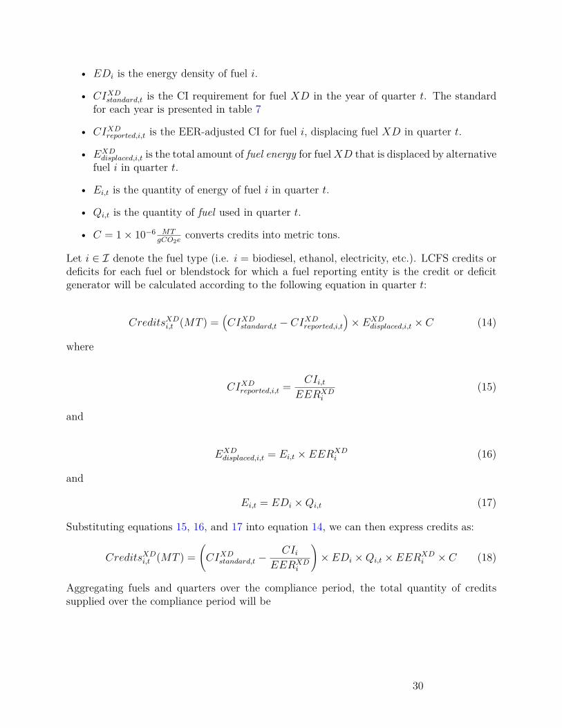
• EDi is the energy density of fuel i.

• CIXDstandard,t is the CI requirement for fuel XD in the year of quarter t. The standardfor each year is presented in table 7

• CIXDreported,i,t is the EER-adjusted CI for fuel i, displacing fuel XD in quarter t.

• EXDdisplaced,i,t is the total amount of fuel energy for fuelXD that is displaced by alternative

fuel i in quarter t.

• Ei,t is the quantity of energy of fuel i in quarter t.

• Qi,t is the quantity of fuel used in quarter t.

• C = 1× 10−6 MTgCO2e

converts credits into metric tons.

Let i ∈ I denote the fuel type (i.e. i = biodiesel, ethanol, electricity, etc.). LCFS credits ordeficits for each fuel or blendstock for which a fuel reporting entity is the credit or deficitgenerator will be calculated according to the following equation in quarter t:

CreditsXDi,t (MT ) =(CIXDstandard,t − CIXDreported,i,t

)× EXD

displaced,i,t × C (14)

where

CIXDreported,i,t = CIi,tEERXD

i

(15)

and

EXDdisplaced,i,t = Ei,t × EERXD

i (16)

and

Ei,t = EDi ×Qi,t (17)

Substituting equations 15, 16, and 17 into equation 14, we can then express credits as:

CreditsXDi,t (MT ) =(CIXDstandard,t −

CIiEERXD

i

)× EDi ×Qi,t × EERXD

i × C (18)

Aggregating fuels and quarters over the compliance period, the total quantity of creditssupplied over the compliance period will be

30

∑i∈I

T∑t=0

CreditsXDi,t (MT ) (19)

=∑i∈I

T∑t=0

(CIXDstandard,t −

CIiEERXD

i

)× EDi ×Qi,t × EERXD

i × C

In the calculations above, deficits are equivalent to negative credits. The compliance period ischaracterized by T , which for our purpose is the fourth quarter of 2030 and t = 0 correspondsto the first quarter of 2019.

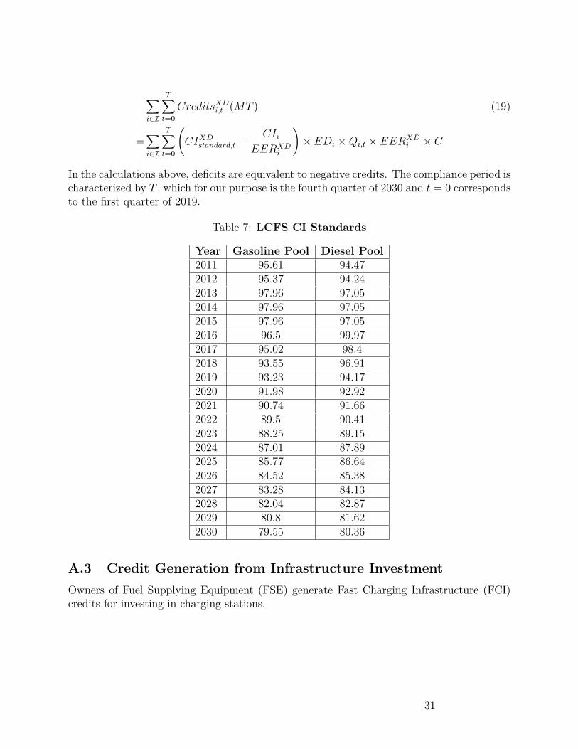
Table 7: LCFS CI Standards

Year Gasoline Pool Diesel Pool2011 95.61 94.472012 95.37 94.242013 97.96 97.052014 97.96 97.052015 97.96 97.052016 96.5 99.972017 95.02 98.42018 93.55 96.912019 93.23 94.172020 91.98 92.922021 90.74 91.662022 89.5 90.412023 88.25 89.152024 87.01 87.892025 85.77 86.642026 84.52 85.382027 83.28 84.132028 82.04 82.872029 80.8 81.622030 79.55 80.36

A.3 Credit Generation from Infrastructure InvestmentOwners of Fuel Supplying Equipment (FSE) generate Fast Charging Infrastructure (FCI)credits for investing in charging stations.

31

FSE owner i generates FCI credits according to:

CreditsiFCI(MT ) =(CIXDstandard × EER− CIFCI

)× Celec (20)

×(CapiFCI ×N × UT − Elecdisp

)× C

where

• CIFCI = CA average grid electricity CI from Lookup Table

• Celec = conversion factor for electricity

• CapiFCI = the (kwH/day) daily FCI charging capacity of FSE i

• N = the number of days during the quarter

• UT = the ‘uptime multiplier’ which is the fraction of time that the FSE is availablefor charging during the quarter

• Elecdisp = the quantity of electricity dispensed (kwH) during the quarter

• EER is for PHEV or electricity/BEV relative to gasoline. Currently this EER = 3.4

A.4 Cap on Total FCI CreditsIn this paper, we assume credits from infrastructure bind at the cap, which is described here.The potential number of credits that can be generated from FCI charging infrastructure iscalculated as:

CreditspotentialFCI = CreditspriorqtrFCI ×(CapapprovedFCI

CapoperationalFCI

)(21)

Applications to generate credits are approved until

CreditspotentialFCI ≥ 0.025×(Deficitspriorqtr

)(22)

A.5 Additional FiguresThis subsection of the appendix contains figures referenced in the text. Figure 8 showsprojections for Brent oil prices, soybean prices, and CA GSP from the BAU simulations.Figure 9 compiles a summary of the ULSD and BBD demand resulting in each compliancescenario, along with the corresponding diesel pool blend rate. Figure 11 shows an aggregatecredit/deficit balance under each compliance scenario, while holding the diesel pool blendrate at 20 percent. This illustrates how many credits would still need to be generated wheneach set of assumptions is assumed.

32

(a) Brent Oil Price (b) GSP

(c) Soybean Prices

Figure 8: Price Forecasts under BAU Uncertainty

33

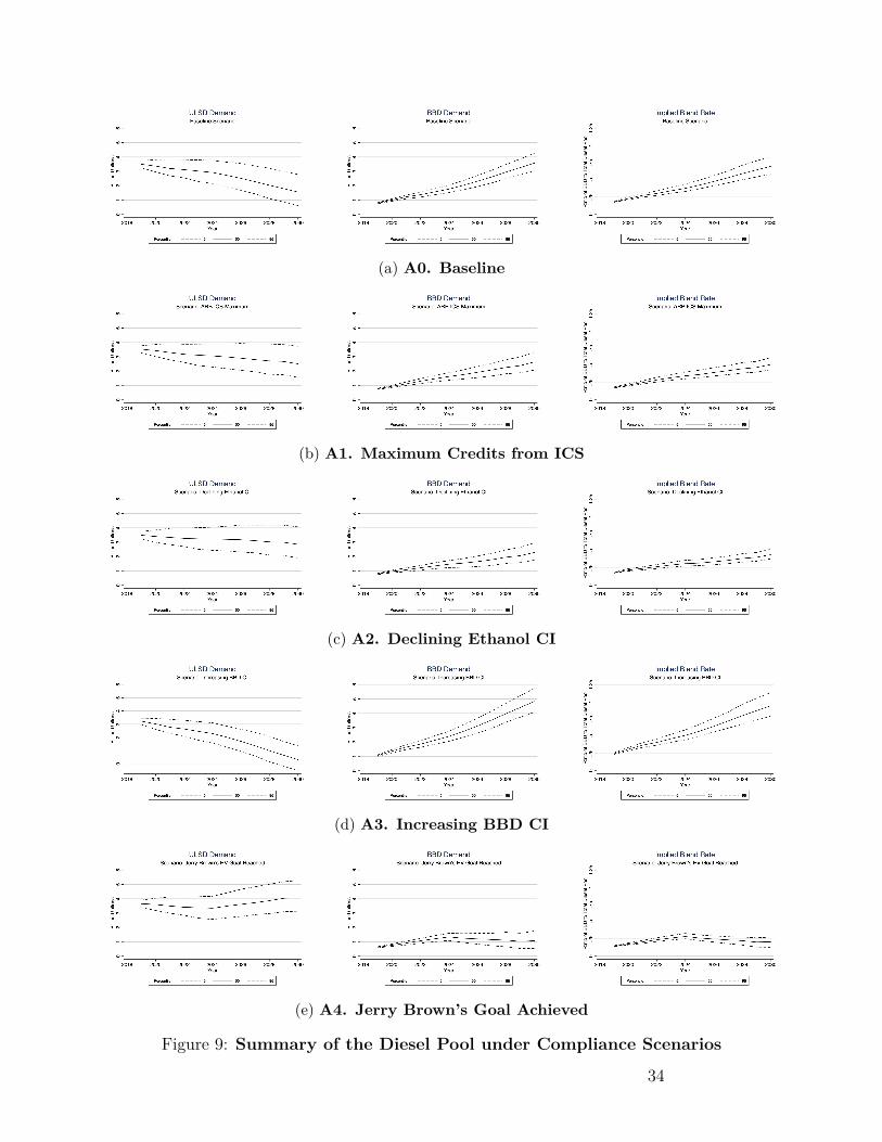
(a) A0. Baseline

(b) A1. Maximum Credits from ICS

(c) A2. Declining Ethanol CI

(d) A3. Increasing BBD CI

(e) A4. Jerry Brown’s Goal Achieved

Figure 9: Summary of the Diesel Pool under Compliance Scenarios

34

Figure 10: Volume-Weighted CI of Ethanol from CARB ICS

35

(a) A0. Baseline (b) A1. ICS Maximum Credits

(c) A2. Declining Ethanol CI (d) A4. Jerry Brown’s Goal Achieved

Figure 11: Summary of Credit Shortages under Different Assumptions

36