cardiac output estimation using arterial blood pressure ...lcp.mit.edu/pdf/sunthesis06.pdf ·...
TRANSCRIPT
Cardiac Output Estimation using Arterial Blood Pressure
Waveforms
by
James Xin Sun
Bachelor of Science in Electrical Engineering and Computer Science (MassachusettsInstitute of Technology, 2005)
Submitted to the Department of Electrical Engineering and Computer Sciencein partial fulfillment of the requirements for the degree of
Master of Engineering in Electrical Engineering and Computer Science
at the
MASSACHUSETTS INSTITUTE OF TECHNOLOGY
September 2006
c© James Xin Sun, MMVI. All rights reserved.
The author hereby grants to MIT permission to reproduce and distribute publiclypaper and electronic copies of this thesis document in whole or in part.
Author . . . . . . . . . . . . . . . . . . . . . . . . . . . . . . . . . . . . . . . . . . . . . . . . . . . . . . . . . . . . . . . . . . . . . . . . . . . .Department of Electrical Engineering and Computer Science
September 1, 2006
Certified by. . . . . . . . . . . . . . . . . . . . . . . . . . . . . . . . . . . . . . . . . . . . . . . . . . . . . . . . . . . . . . . . . . . . . . . .Roger G. Mark
Distinguished Professor in Health Sciences and TechnologyProfessor of Electrical Engineering
Thesis Supervisor
Accepted by . . . . . . . . . . . . . . . . . . . . . . . . . . . . . . . . . . . . . . . . . . . . . . . . . . . . . . . . . . . . . . . . . . . . . . .Arthur C. Smith
Chairman, Department Committee on Graduate Students

2
Cardiac Output Estimation using Arterial Blood Pressure Waveformsby
James Xin Sun
Submitted to the Department of Electrical Engineering and Computer Scienceon September 1, 2006, in partial fulfillment of the
requirements for the degree ofMaster of Engineering in Electrical Engineering and Computer Science
Abstract
Cardiac output (CO) is a cardinal parameter of cardiovascular state, and a fundamentaldeterminant of global oxygen delivery. Historically, measurement of CO has been limitedto critically-ill patients, using invasive indicator-dilution methods such as thermodilutionvia Swan-Ganz lines, which carry risks. Over the past century, the premise that CO couldbe estimated by analysis of the arterial blood pressure (ABP) waveform has captured theattention of many investigators. This approach of estimating CO is minimally invasive,cheap, and can be done continuously as long as ABP waveforms are available. Over a dozendifferent methods of estimating CO from ABP waveforms have been proposed and someare commercialized. However, the effectiveness of this approach is nebular. Performancevalidation studies in the past have mostly been conducted on a small set of subjects underwell-controlled laboratory conditions. It is entirely possible that there will be circumstancesin real world clinical practice in which CO estimation produces inaccurate results.
In this thesis, our goals are to (1) build a computational system that estimates COusing 11 of the established methods; (2) evaluate and compare the performance of the COestimation methods on a large set clinical data, using the simultaneously available ther-modilution CO measurements as gold-standard; and (3) design and evaluate an algorithmthat identifies and eliminates ABP waveform segments of poor quality.
Out of the 11 CO estimation methods studied, there is one method (Liljestrand method)that is clearly more accurate than the rest. Across our study population of 120 subjects, theLiljestrand method has an error distribution with a 1 standard deviation error of 0.8 L/min,which is roughly twice that of thermodilution CO. These results suggest that although COestimation methods may not generate the most precise values, they are still useful fordetecting significant (>1 L/min) changes in CO.
Thesis Supervisor: Roger G. MarkTitle: Distinguished Professor in Health Sciences and TechnologyProfessor of Electrical Engineering
3

4

Acknowledgments
This research would not have been possible without the help and support of many people.First, I thank my thesis supervisor, Prof. Roger G. Mark. Your advice, support, care,
and friendship are the reasons for the success of this thesis. Your leadership is truly inspiring.You have opened my eyes to the vast field of biomedical engineering, and I fully intend topursue this field for the rest of my life.
I owe a great deal to Dr. Andrew Reisner and Mohammed Saeed. They introduced meto the area of cardiac output estimation. Their help and support unquestionably shapedthe scope of my research.
I thank all members of the Lab for Computational Physiology and members of theBRP. It is because of them I enjoyed being at the lab almost every day. Thanks to Dr. GariClifford for all the signal processing advice and his British sense of humor; to Dr. ThomasHeldt for his technical advice and of course, for his self-confident attitude; to Tushar Parlikarfor keeping this final semester so entertaining; to Mauricio Villarroel, the UNIX guru, forthe database and Linux support; to Anton Aboukhalil for his magic tricks.
I thank all my friends at MIT. Dearest thanks to every member of the “little-family”for all those get-togethers and birthday showerings: I will treasure all those memorablemoments; to Tin, the “free electricity” Burmese, for being a great friend and lab-mate atLCP.
I sincerely thank my family (mom, dad, Andrew) for all their encouragement, love, andsupport.
This work was made possible by grant R01 EB001659 from the National Institute ofBiomedical Imaging and Bioengineering.
5

6

Contents
1 Introduction 13
1.1 Motivation . . . . . . . . . . . . . . . . . . . . . . . . . . . . . . . . . . . . 13
1.1.1 Measurement of cardiac output . . . . . . . . . . . . . . . . . . . . . 13
1.1.2 Estimating cardiac output from arterial blood pressure . . . . . . . . 16
1.1.3 MIMIC II database & data quality . . . . . . . . . . . . . . . . . . . 16
1.2 Thesis goals . . . . . . . . . . . . . . . . . . . . . . . . . . . . . . . . . . . . 17
1.3 Thesis outline . . . . . . . . . . . . . . . . . . . . . . . . . . . . . . . . . . . 17
2 Cardiac Output Estimation Theory 19
2.1 Lumped parameter methods . . . . . . . . . . . . . . . . . . . . . . . . . . . 20
2.1.1 Mean arterial pressure . . . . . . . . . . . . . . . . . . . . . . . . . . 20
2.1.2 Windkessel model [5] . . . . . . . . . . . . . . . . . . . . . . . . . . . 20
2.1.3 Windkessel RC decay [4] . . . . . . . . . . . . . . . . . . . . . . . . . 21
2.1.4 Herd [7] . . . . . . . . . . . . . . . . . . . . . . . . . . . . . . . . . . 21
2.1.5 Liljestrand nonlinear compliance [12] . . . . . . . . . . . . . . . . . . 21
2.2 Pressure-area methods . . . . . . . . . . . . . . . . . . . . . . . . . . . . . . 21
2.2.1 Systolic area [19] . . . . . . . . . . . . . . . . . . . . . . . . . . . . . 22
2.2.2 Systolic area with correction [19, 10] . . . . . . . . . . . . . . . . . . 22
2.2.3 Systolic area with corrected impedance [21] . . . . . . . . . . . . . . 22
2.2.4 Pressure root-mean-square [9] . . . . . . . . . . . . . . . . . . . . . . 22
2.3 Lumped-parameter, instantaneous flow methods . . . . . . . . . . . . . . . 24
2.3.1 Godje nonlinear compliance [6] . . . . . . . . . . . . . . . . . . . . . 24
2.3.2 Wesseling Modelflow [20] . . . . . . . . . . . . . . . . . . . . . . . . 25
2.4 Limitations of CO estimation . . . . . . . . . . . . . . . . . . . . . . . . . . 25
3 Signal Abnormality Indexing 27
3.1 Introduction . . . . . . . . . . . . . . . . . . . . . . . . . . . . . . . . . . . . 27
3.2 Methods . . . . . . . . . . . . . . . . . . . . . . . . . . . . . . . . . . . . . . 27
3.2.1 Feature extraction . . . . . . . . . . . . . . . . . . . . . . . . . . . . 29
3.2.2 Abnormality indexing . . . . . . . . . . . . . . . . . . . . . . . . . . 29
3.2.3 Algorithm evaluation . . . . . . . . . . . . . . . . . . . . . . . . . . . 30
3.3 Results . . . . . . . . . . . . . . . . . . . . . . . . . . . . . . . . . . . . . . . 32
3.3.1 SAI versus human . . . . . . . . . . . . . . . . . . . . . . . . . . . . 32
3.3.2 Sensitivity analysis . . . . . . . . . . . . . . . . . . . . . . . . . . . . 32
3.3.3 Cardiac output estimation error . . . . . . . . . . . . . . . . . . . . 33
3.4 Discussion and conclusions . . . . . . . . . . . . . . . . . . . . . . . . . . . . 33
7
4 Evaluation Methods 35
4.1 Data extraction . . . . . . . . . . . . . . . . . . . . . . . . . . . . . . . . . . 364.2 Implementation of CO estimators . . . . . . . . . . . . . . . . . . . . . . . . 36
4.2.1 ABP beat detection . . . . . . . . . . . . . . . . . . . . . . . . . . . 364.2.2 ABP feature extraction . . . . . . . . . . . . . . . . . . . . . . . . . 374.2.3 CO estimator implementation . . . . . . . . . . . . . . . . . . . . . . 384.2.4 Signal quality and bad beats elimination . . . . . . . . . . . . . . . . 384.2.5 Running-average LPF to reduce beat-to-beat fluctuations . . . . . . 40
4.3 Comparing estimated CO to gold-standard CO . . . . . . . . . . . . . . . . 404.3.1 Averaging beat-to-beat CO estimates . . . . . . . . . . . . . . . . . 414.3.2 Calibration techniques . . . . . . . . . . . . . . . . . . . . . . . . . . 414.3.3 Relative CO estimation . . . . . . . . . . . . . . . . . . . . . . . . . 42
4.4 Error analysis . . . . . . . . . . . . . . . . . . . . . . . . . . . . . . . . . . . 43
5 Results and Discussion 47
5.1 Subject population statistics . . . . . . . . . . . . . . . . . . . . . . . . . . . 475.2 Removal of poor quality waveforms . . . . . . . . . . . . . . . . . . . . . . . 475.3 Absolute CO estimation . . . . . . . . . . . . . . . . . . . . . . . . . . . . . 495.4 Variability of calibration constants . . . . . . . . . . . . . . . . . . . . . . . 535.5 Variability of CO estimates . . . . . . . . . . . . . . . . . . . . . . . . . . . 535.6 Relative CO estimation . . . . . . . . . . . . . . . . . . . . . . . . . . . . . 545.7 Error analysis of selected CO estimators . . . . . . . . . . . . . . . . . . . . 545.8 Selected time series case studies . . . . . . . . . . . . . . . . . . . . . . . . . 605.9 Discussion . . . . . . . . . . . . . . . . . . . . . . . . . . . . . . . . . . . . . 60
6 Conclusions and Future Research 63
6.1 Summary . . . . . . . . . . . . . . . . . . . . . . . . . . . . . . . . . . . . . 636.2 Suggestions for future research . . . . . . . . . . . . . . . . . . . . . . . . . 64
A Notation Summary 65
B Selected Code Descriptions 67
B.1 wavex.m . . . . . . . . . . . . . . . . . . . . . . . . . . . . . . . . . . . . . . 67B.2 trendex.m . . . . . . . . . . . . . . . . . . . . . . . . . . . . . . . . . . . . . 67B.3 wabp.m . . . . . . . . . . . . . . . . . . . . . . . . . . . . . . . . . . . . . . 68B.4 abpfeature.m . . . . . . . . . . . . . . . . . . . . . . . . . . . . . . . . . . . 68B.5 jSQI.m . . . . . . . . . . . . . . . . . . . . . . . . . . . . . . . . . . . . . . . 68B.6 estimateCO.m . . . . . . . . . . . . . . . . . . . . . . . . . . . . . . . . . . . 69
C Test of Statistical Significance 71
8
List of Figures
1-1 Cardiovascular system. . . . . . . . . . . . . . . . . . . . . . . . . . . . . . . 14
1-2 Indicator dilution principle. . . . . . . . . . . . . . . . . . . . . . . . . . . . 15
1-3 ABP waveform. . . . . . . . . . . . . . . . . . . . . . . . . . . . . . . . . . . 16
1-4 Cardiovascular system. . . . . . . . . . . . . . . . . . . . . . . . . . . . . . . 17
2-1 Mean arterial pressure Pm and cardiac output Q. . . . . . . . . . . . . . . . 20
2-2 The Windkessel RC circuit model. . . . . . . . . . . . . . . . . . . . . . . . 20
2-3 Windkessel model with nonlinear capacitor. . . . . . . . . . . . . . . . . . . 22
2-4 Arterial tree of a dog. . . . . . . . . . . . . . . . . . . . . . . . . . . . . . . 23
2-5 A transmission line circuit. . . . . . . . . . . . . . . . . . . . . . . . . . . . 23
2-6 Pressure-area during systole. . . . . . . . . . . . . . . . . . . . . . . . . . . 24
2-7 Godje model with nonlinear capacitance and aortic impedance terms. . . . 24
2-8 Wesseling’s modelflow model. . . . . . . . . . . . . . . . . . . . . . . . . . . 25
2-9 Pressure waveforms in aorta versus radial artery. . . . . . . . . . . . . . . . 25
3-1 Damped ABP waveform. . . . . . . . . . . . . . . . . . . . . . . . . . . . . . 28
3-2 ABP waveform with disturbance. . . . . . . . . . . . . . . . . . . . . . . . . 28
3-3 Noisy ABP waveform. . . . . . . . . . . . . . . . . . . . . . . . . . . . . . . 28
3-4 Example of SAI . . . . . . . . . . . . . . . . . . . . . . . . . . . . . . . . . . 29
3-5 SAI block diagram. . . . . . . . . . . . . . . . . . . . . . . . . . . . . . . . . 29
3-6 SAI parameter sensitivity. . . . . . . . . . . . . . . . . . . . . . . . . . . . . 32
3-7 CO estimation error as a function of maximum accepted cSAI . . . . . . . . 34
4-1 A system for evaluating CO estimation performance. . . . . . . . . . . . . . 36
4-2 Data flow diagram for CO estimation. . . . . . . . . . . . . . . . . . . . . . 36
4-3 The slope sum function . . . . . . . . . . . . . . . . . . . . . . . . . . . . . 37
4-4 Ps, Pd, and Pp detection . . . . . . . . . . . . . . . . . . . . . . . . . . . . . 38
4-5 The cardiac cycle. . . . . . . . . . . . . . . . . . . . . . . . . . . . . . . . . 39
4-6 End of systole and systolic area . . . . . . . . . . . . . . . . . . . . . . . . . 39
4-7 Beat-to-beat variability in ABP waveform. . . . . . . . . . . . . . . . . . . . 40
4-8 Window size for averaging CO estimates. . . . . . . . . . . . . . . . . . . . 41
4-9 Vector visualization of TCO and estimated CO . . . . . . . . . . . . . . . . 42
4-10 Bland-Altman plot . . . . . . . . . . . . . . . . . . . . . . . . . . . . . . . . 43
4-11 Percentage changes in TCO versus estimated CO. . . . . . . . . . . . . . . . 45
5-1 Population statistics . . . . . . . . . . . . . . . . . . . . . . . . . . . . . . . 48
5-2 Bland Altman plot . . . . . . . . . . . . . . . . . . . . . . . . . . . . . . . . 50
5-3 Bland-Altman error analysis plots. . . . . . . . . . . . . . . . . . . . . . . . 51
5-4 Bland-Altman error analysis plots (continued). . . . . . . . . . . . . . . . . 52
9

5-5 Performance of percentages changes in CO. . . . . . . . . . . . . . . . . . . 555-6 Performance of percentages changes in CO (continued). . . . . . . . . . . . 565-7 CO estimation (Liljestrand) error as functions of several variables. . . . . . 575-8 CO estimation (MAP) error as functions of several variables (MAP). . . . . 585-9 CO estimation (Modelflow) error as functions of several variables. . . . . . . 595-10 Time series of caseID 8463 using the Liljestrand CO estimator. . . . . . . . 615-11 Time series of caseID 6629 using the Liljestrand CO estimator. . . . . . . . 62
10

List of Tables
2.1 Cardiac output estimators . . . . . . . . . . . . . . . . . . . . . . . . . . . . 19
3.1 ABP features . . . . . . . . . . . . . . . . . . . . . . . . . . . . . . . . . . . 303.2 SAI logic . . . . . . . . . . . . . . . . . . . . . . . . . . . . . . . . . . . . . 303.3 CO estimators taken from Table 2.1. . . . . . . . . . . . . . . . . . . . . . . 313.4 SAI versus human: distribution . . . . . . . . . . . . . . . . . . . . . . . . . 323.5 SAI versus human: statistical summary . . . . . . . . . . . . . . . . . . . . 323.6 SAI sensitivity . . . . . . . . . . . . . . . . . . . . . . . . . . . . . . . . . . 33
4.1 ABP features . . . . . . . . . . . . . . . . . . . . . . . . . . . . . . . . . . . 37
5.1 Population statistics . . . . . . . . . . . . . . . . . . . . . . . . . . . . . . . 475.2 Estimation error in L/min at 1 SD with 3 different calibration methods. . . 495.3 Variability of k for C1 and C3 calibration. . . . . . . . . . . . . . . . . . . . 535.4 Variability of CO estimates. . . . . . . . . . . . . . . . . . . . . . . . . . . . 535.5 Relative CO estimation error. . . . . . . . . . . . . . . . . . . . . . . . . . . 54
A.1 Commonly used acronyms and symbols . . . . . . . . . . . . . . . . . . . . 65
C.1 p-values using the Kolmogorov-Smirnov test. . . . . . . . . . . . . . . . . . 71C.2 Labels for CO estimation methods. . . . . . . . . . . . . . . . . . . . . . . . 71
11

12
Chapter 1
Introduction
1.1 Motivation
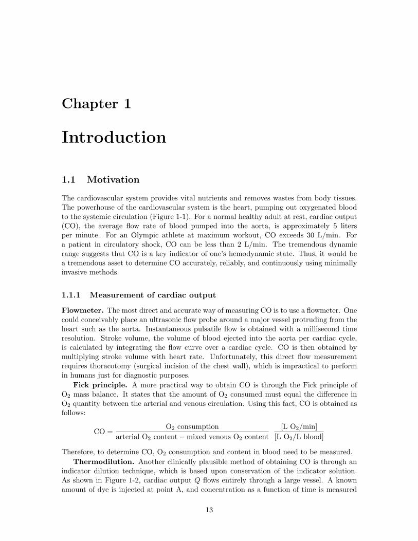
The cardiovascular system provides vital nutrients and removes wastes from body tissues.The powerhouse of the cardiovascular system is the heart, pumping out oxygenated bloodto the systemic circulation (Figure 1-1). For a normal healthy adult at rest, cardiac output(CO), the average flow rate of blood pumped into the aorta, is approximately 5 litersper minute. For an Olympic athlete at maximum workout, CO exceeds 30 L/min. Fora patient in circulatory shock, CO can be less than 2 L/min. The tremendous dynamicrange suggests that CO is a key indicator of one’s hemodynamic state. Thus, it would bea tremendous asset to determine CO accurately, reliably, and continuously using minimallyinvasive methods.
1.1.1 Measurement of cardiac output
Flowmeter. The most direct and accurate way of measuring CO is to use a flowmeter. Onecould conceivably place an ultrasonic flow probe around a major vessel protruding from theheart such as the aorta. Instantaneous pulsatile flow is obtained with a millisecond timeresolution. Stroke volume, the volume of blood ejected into the aorta per cardiac cycle,is calculated by integrating the flow curve over a cardiac cycle. CO is then obtained bymultiplying stroke volume with heart rate. Unfortunately, this direct flow measurementrequires thoracotomy (surgical incision of the chest wall), which is impractical to performin humans just for diagnostic purposes.
Fick principle. A more practical way to obtain CO is through the Fick principle ofO2 mass balance. It states that the amount of O2 consumed must equal the difference inO2 quantity between the arterial and venous circulation. Using this fact, CO is obtained asfollows:
CO =O2 consumption
arterial O2 content − mixed venous O2 content
[L O2/min]
[L O2/L blood]
Therefore, to determine CO, O2 consumption and content in blood need to be measured.
Thermodilution. Another clinically plausible method of obtaining CO is through anindicator dilution technique, which is based upon conservation of the indicator solution.As shown in Figure 1-2, cardiac output Q flows entirely through a large vessel. A knownamount of dye is injected at point A, and concentration as a function of time is measured
13

Figure 1-1: The cardiovascular system. Figure adapted from [13].
14

downstream at point B. By dye conservation, the amount injected must pass through pointB, and CO is obtained as follows:
CO =q
∫ t2t1
c(t)dt
[mg]
[mg·min/(L blood)]
Clinically, the most popular indicator dilution technique is thermodilution, in which coldsaline of precisely known volume and temperature is injected, and then the temperatureprofile is measured downstream.
Figure 1-2: Indicator dilution principle. Figure adapted from [2].
Doppler ultrasound. More recently, a completely noninvasive method known asdoppler ultrasound has been developed to measure CO [8]. This technique measures theaorta’s instantaneous blood flow velocity v(t) and cross sectional area A. Then strokevolume can be calculated by integrating v(t) over a cardiac cycle of duration T :
SV = A
∫
Tv(t)dt
Remarks. Although the Fick method and thermodilution are both clinically feasible,they are still quite invasive and can only be performed in well-equipped environments likeintensive care units (ICUs) and cardiac catheterization labs. Measurement of mixed venousO2 requires a blood sample from the pulmonary artery. Injection of cold saline must be intoa major vessel through which the entire CO flows. Consequently, a Swan-Ganz catheterthat is threaded through the vena cava, through the right heart, and into the pulmonaryartery is used to facilitate thermodilution CO measurements. Doppler ultrasound, whilecompletely noninvasive and reasonably accurate, is expensive. Running this device requirescostly equipment and an expert technician. In addition, none of the methods discussed inthis section are practical for continuous bedside monitoring of a patient’s CO.
15
1.1.2 Estimating cardiac output from arterial blood pressure
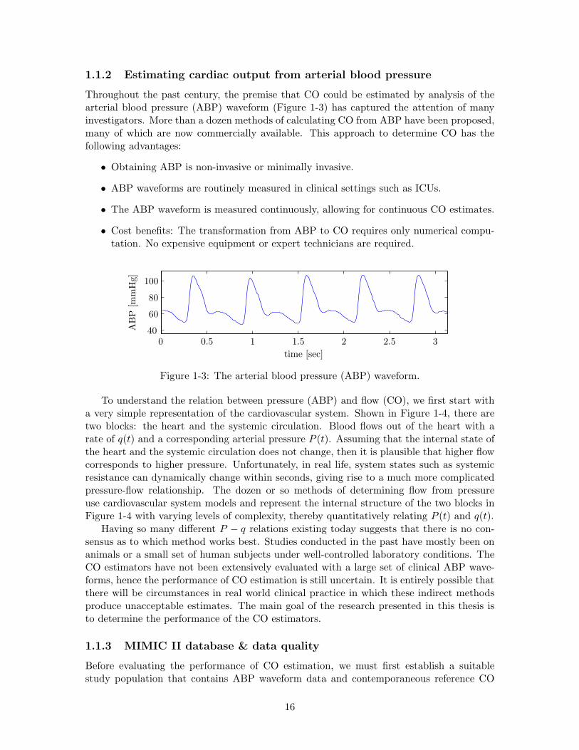
Throughout the past century, the premise that CO could be estimated by analysis of thearterial blood pressure (ABP) waveform (Figure 1-3) has captured the attention of manyinvestigators. More than a dozen methods of calculating CO from ABP have been proposed,many of which are now commercially available. This approach to determine CO has thefollowing advantages:
• Obtaining ABP is non-invasive or minimally invasive.
• ABP waveforms are routinely measured in clinical settings such as ICUs.
• The ABP waveform is measured continuously, allowing for continuous CO estimates.
• Cost benefits: The transformation from ABP to CO requires only numerical compu-tation. No expensive equipment or expert technicians are required.
time [sec]
AB
P[m
mH
g]
0 0.5 1 1.5 2 2.5 340
60
80
100
Figure 1-3: The arterial blood pressure (ABP) waveform.
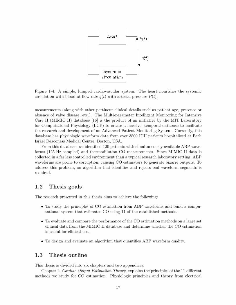
To understand the relation between pressure (ABP) and flow (CO), we first start witha very simple representation of the cardiovascular system. Shown in Figure 1-4, there aretwo blocks: the heart and the systemic circulation. Blood flows out of the heart with arate of q(t) and a corresponding arterial pressure P (t). Assuming that the internal state ofthe heart and the systemic circulation does not change, then it is plausible that higher flowcorresponds to higher pressure. Unfortunately, in real life, system states such as systemicresistance can dynamically change within seconds, giving rise to a much more complicatedpressure-flow relationship. The dozen or so methods of determining flow from pressureuse cardiovascular system models and represent the internal structure of the two blocks inFigure 1-4 with varying levels of complexity, thereby quantitatively relating P (t) and q(t).
Having so many different P − q relations existing today suggests that there is no con-sensus as to which method works best. Studies conducted in the past have mostly been onanimals or a small set of human subjects under well-controlled laboratory conditions. TheCO estimators have not been extensively evaluated with a large set of clinical ABP wave-forms, hence the performance of CO estimation is still uncertain. It is entirely possible thatthere will be circumstances in real world clinical practice in which these indirect methodsproduce unacceptable estimates. The main goal of the research presented in this thesis isto determine the performance of the CO estimators.
1.1.3 MIMIC II database & data quality
Before evaluating the performance of CO estimation, we must first establish a suitablestudy population that contains ABP waveform data and contemporaneous reference CO
16
�������������������
��������Figure 1-4: A simple, lumped cardiovascular system. The heart nourishes the systemiccirculation with blood at flow rate q(t) with arterial pressure P (t).
measurements (along with other pertinent clinical details such as patient age, presence orabsence of valve disease, etc.). The Multi-parameter Intelligent Monitoring for IntensiveCare II (MIMIC II) database [16] is the product of an initiative by the MIT Laboratoryfor Computational Physiology (LCP) to create a massive, temporal database to facilitatethe research and development of an Advanced Patient Monitoring System. Currently, thisdatabase has physiologic waveform data from over 3500 ICU patients hospitalized at BethIsrael Deaconess Medical Center, Boston, USA.
From this database, we identified 120 patients with simultaneously available ABP wave-forms (125-Hz sampled) and thermodilution CO measurements. Since MIMIC II data iscollected in a far less controlled environment than a typical research laboratory setting, ABPwaveforms are prone to corruption, causing CO estimators to generate bizarre outputs. Toaddress this problem, an algorithm that identifies and rejects bad waveform segments isrequired.
1.2 Thesis goals
The research presented in this thesis aims to achieve the following:
• To study the principles of CO estimation from ABP waveforms and build a compu-tational system that estimates CO using 11 of the established methods.
• To evaluate and compare the performance of the CO estimation methods on a large setclinical data from the MIMIC II database and determine whether the CO estimationis useful for clinical use.
• To design and evaluate an algorithm that quantifies ABP waveform quality.
1.3 Thesis outline
This thesis is divided into six chapters and two appendices.
Chapter 2, Cardiac Output Estimation Theory, explains the principles of the 11 differentmethods we study for CO estimation. Physiologic principles and theory from electrical
17
circuits are used whenever appropriate to provide intuition. Limitations of CO estimationare also discussed.
Chapter 3, Signal Abnormality Indexing, addresses the key issue of ABP waveformquality. CO estimation relies on a clean ABP waveform, in which pressure and temporalfeatures may be reliably obtained. This chapter discusses the design and evaluation of analgorithm that flags poor quality ABP waveforms.
Chapter 4, Evaluation Methods, explains the computational system built to evaluate COestimation, which involves database extraction, ABP waveform processing, CO estimatorimplementation, and performance evaluation.
Chapter 5, Results and Discussion, reports the performance of CO estimation. Wediscuss subset error analysis to determine the physiologic situations in which CO estimatorsare likely to be more erroneous.
Chapter 6, Conclusions and Future Research, summarizes the important findings fromthis research and suggests possible areas worthy of further exploration.
Appendix A presents a table summarizing the acronyms and mathematical notationsused throughout this thesis. Appendix B contains input/output relations of importantMATLAB source code to help elucidate Chapter 4.
18
Chapter 2
Cardiac Output Estimation Theory
In the cardiovascular system, the relationship between arterial blood pressure (ABP) andcardiac output (CO) is quite complex. Over a dozen methods of estimating flow from pres-sure have been proposed. Most of the methods operate at a beat-by-beat time resolution,calculating the stroke volume of each beat. Then, CO is calculated by multiplying strokevolume with heart rate. The bases of these methods are models of the systemic circulation.
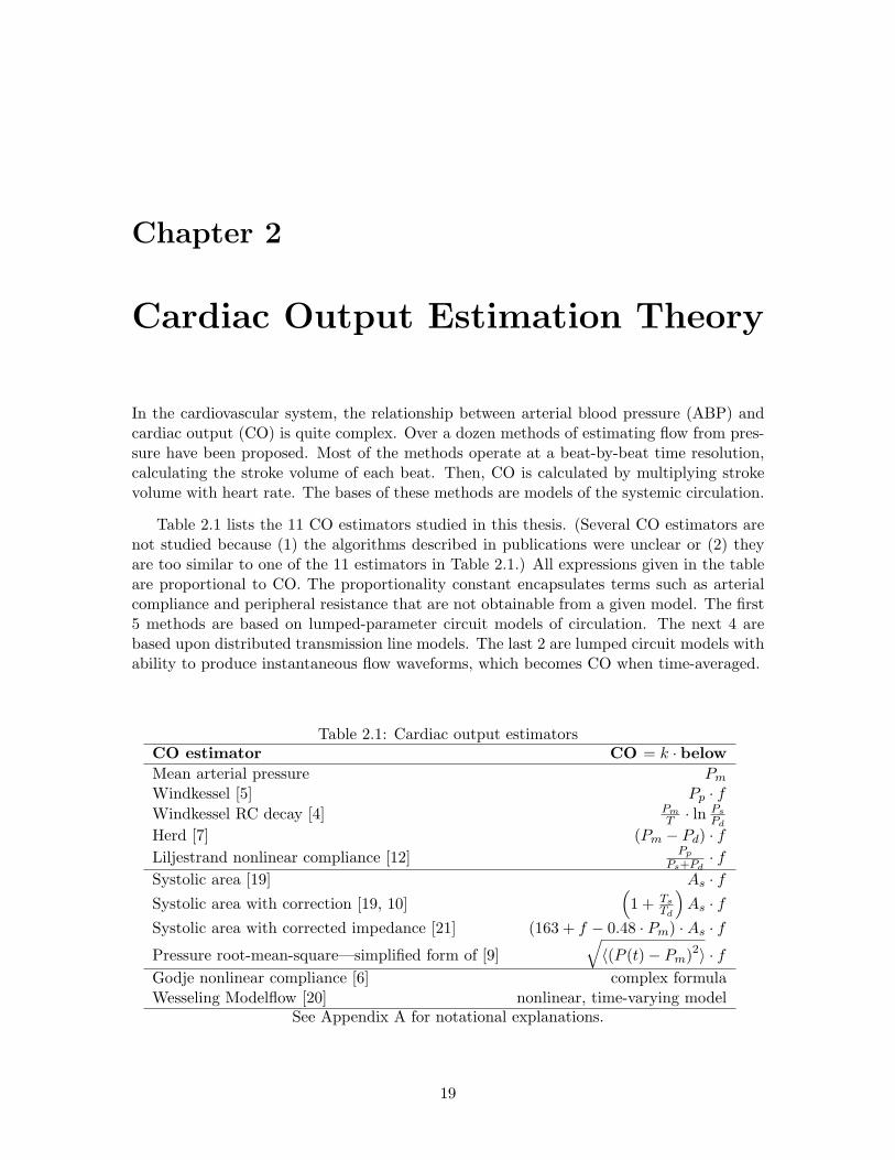
Table 2.1 lists the 11 CO estimators studied in this thesis. (Several CO estimators arenot studied because (1) the algorithms described in publications were unclear or (2) theyare too similar to one of the 11 estimators in Table 2.1.) All expressions given in the tableare proportional to CO. The proportionality constant encapsulates terms such as arterialcompliance and peripheral resistance that are not obtainable from a given model. The first5 methods are based on lumped-parameter circuit models of circulation. The next 4 arebased upon distributed transmission line models. The last 2 are lumped circuit models withability to produce instantaneous flow waveforms, which becomes CO when time-averaged.
Table 2.1: Cardiac output estimatorsCO estimator CO = k · below
Mean arterial pressure Pm
Windkessel [5] Pp · fWindkessel RC decay [4] Pm
T · ln Ps
Pd
Herd [7] (Pm − Pd) · fLiljestrand nonlinear compliance [12]
Pp
Ps+Pd· f
Systolic area [19] As · fSystolic area with correction [19, 10]
(
1 + Ts
Td
)
As · fSystolic area with corrected impedance [21] (163 + f − 0.48 · Pm) · As · fPressure root-mean-square—simplified form of [9]
√
〈(P (t) − Pm)2〉 · fGodje nonlinear compliance [6] complex formulaWesseling Modelflow [20] nonlinear, time-varying model
See Appendix A for notational explanations.
19
2.1 Lumped parameter methods
2.1.1 Mean arterial pressure
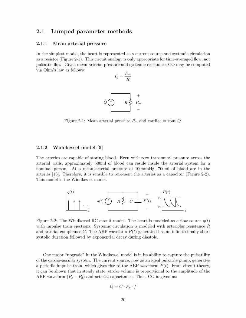
In the simplest model, the heart is represented as a current source and systemic circulationas a resistor (Figure 2-1). This circuit analogy is only appropriate for time-averaged flow, notpulsatile flow. Given mean arterial pressure and systemic resistance, CO may be computedvia Ohm’s law as follows:
Q =Pm
R
Q R Pm
+
−
Figure 2-1: Mean arterial pressure Pm and cardiac output Q.
2.1.2 Windkessel model [5]
The arteries are capable of storing blood. Even with zero transmural pressure across thearterial walls, approximately 500ml of blood can reside inside the arterial system for anominal person. At a mean arterial pressure of 100mmHg, 700ml of blood are in thearteries [13]. Therefore, it is sensible to represent the arteries as a capacitor (Figure 2-2).This model is the Windkessel model.
q(t)
t· · ·
P (t)
t
Ps
Pd
q(t) R C P (t)
+
−
Figure 2-2: The Windkessel RC circuit model. The heart is modeled as a flow source q(t)with impulse train ejections. Systemic circulation is modeled with arteriolar resistance Rand arterial compliance C. The ABP waveform P (t) generated has an infinitesimally shortsystolic duration followed by exponential decay during diastole.
One major “upgrade” in the Windkessel model is in its ability to capture the pulsatilityof the cardiovascular system. The current source, now as an ideal pulsatile pump, generatesa periodic impulse train, which gives rise to the ABP waveform P (t). From circuit theory,it can be shown that in steady state, stroke volume is proportional to the amplitude of theABP waveform (Ps − Pd) and arterial capacitance. Thus, CO is given as:
Q = C · Pp · f
20
2.1.3 Windkessel RC decay [4]
If the time constant τ of the Windkessel RC circuit model is known, then cardiac outputmay be computed in another way:
Q =Pm
R= C · Pm
RC= C · Pm
τ
There are several methods to determine τ :
• Use the Windkessel idealization that ejection is instantaneous. This way, the entirecardiac cycle is in exponential decay from systolic to diastolic pressure. Mathemati-cally,
Pd = Pse−T/τ
where T is the beat period. Solving for τ , we obtain:
τ =T
ln Ps
Pd
Hence, the final CO expression:
Q = C · Pm
T· ln Ps
Pd
• Perform a least squares fit of an exponential decay to the diastole portion of the ABPwaveform. Then, the best-fitted τ is obtained.
• Use a refined exponential fitting technique by Mukkamula et al. [14].
In this thesis, τ is obtained separately using the first two methods.
2.1.4 Herd [7]
The Herd method proposes that stroke volume is proportional to Pm−Pd. This methodologyis based upon empirical evidence and no physiologic intuition is given [7].
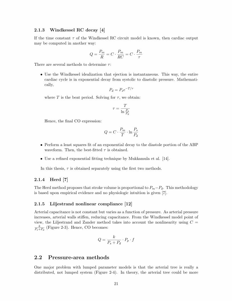
2.1.5 Liljestrand nonlinear compliance [12]
Arterial capacitance is not constant but varies as a function of pressure. As arterial pressureincreases, arterial walls stiffen, reducing capacitance. From the Windkessel model point ofview, the Liljestrand and Zander method takes into account the nonlinearity using C =
kPs+Pd
(Figure 2-3). Hence, CO becomes:
Q =k
Ps + Pd· Pp · f
2.2 Pressure-area methods
One major problem with lumped parameter models is that the arterial tree is really adistributed, not lumped system (Figure 2-4). In theory, the arterial tree could be more
21
q(t) R C P (t)
+
−
Figure 2-3: Windkessel model with nonlinear capacitor. Liljestrand and Zander proposethat C ∝ (Ps + Pd)
−1.
accurately modeled using the transmission line circuitry, which captures the distributednature and associated effects such as impedance and wave reflections. Although none ofthe pressure-area methods are explicitly derived from transmission line circuit theory, thearterial tree is approached from a distributed system point of view.
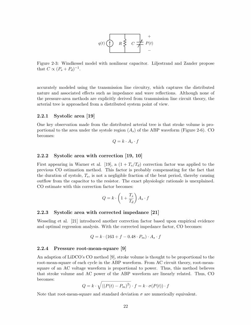
2.2.1 Systolic area [19]
One key observation made from the distributed arterial tree is that stroke volume is pro-portional to the area under the systole region (As) of the ABP waveform (Figure 2-6). CObecomes:
Q = k · As · f
2.2.2 Systolic area with correction [19, 10]
First appearing in Warner et al. [19], a (1 + Ts/Td) correction factor was applied to theprevious CO estimation method. This factor is probably compensating for the fact thatthe duration of systole, Ts, is not a negligible fraction of the beat period, thereby causingoutflow from the capacitor to the resistor. The exact physiologic rationale is unexplained.CO estimate with this correction factor becomes:
Q = k ·(
1 +Ts
Td
)
As · f
2.2.3 Systolic area with corrected impedance [21]
Wesseling et al. [21] introduced another correction factor based upon empirical evidenceand optimal regression analysis. With the corrected impedance factor, CO becomes:
Q = k · (163 + f − 0.48 · Pm) · As · f
2.2.4 Pressure root-mean-square [9]
An adaption of LiDCO’s CO method [9], stroke volume is thought to be proportional to theroot-mean-square of each cycle in the ABP waveform. From AC circuit theory, root-mean-square of an AC voltage waveform is proportional to power. Thus, this method believesthat stroke volume and AC power of the ABP waveform are linearly related. Thus, CObecomes:
Q = k ·√
〈(P (t) − Pm)2〉 · f = k · σ(P (t)) · fNote that root-mean-square and standard deviation σ are numerically equivalent.
22
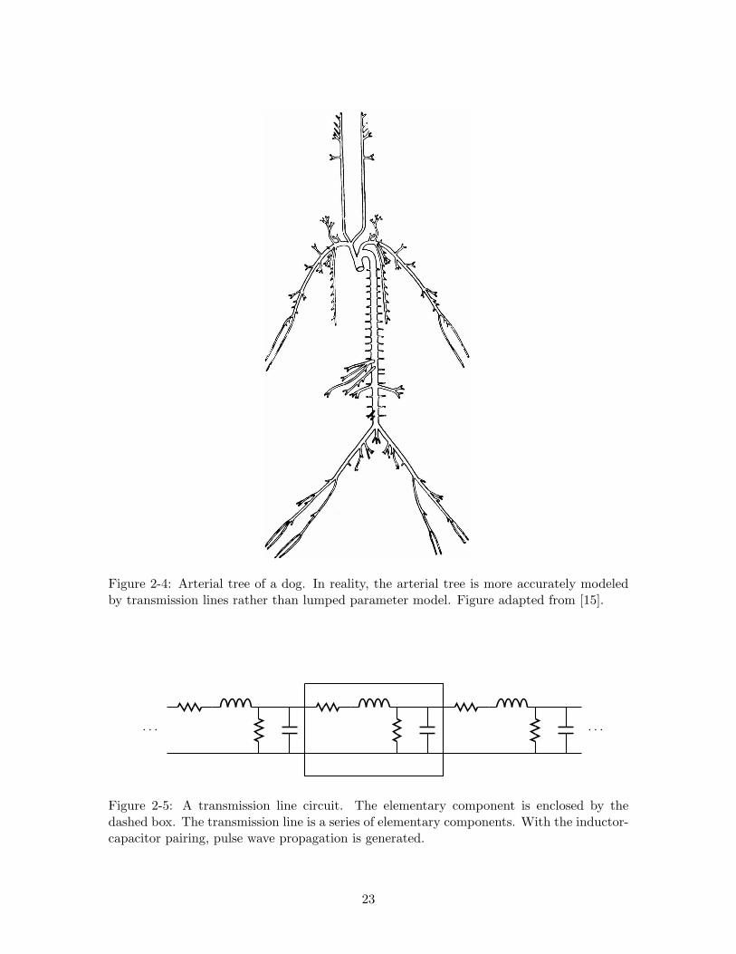
Figure 2-4: Arterial tree of a dog. In reality, the arterial tree is more accurately modeledby transmission lines rather than lumped parameter model. Figure adapted from [15].
· · · · · ·
Figure 2-5: A transmission line circuit. The elementary component is enclosed by thedashed box. The transmission line is a series of elementary components. With the inductor-capacitor pairing, pulse wave propagation is generated.
23

Figure 2-6: Pressure-area during systole. One cycle of the ABP waveform is shown. Strokevolume is believed to be proportional to the area of the shaded region. Figure adapted from[10].
2.3 Lumped-parameter, instantaneous flow methods
Two of the CO estimation methods investigated in this thesis use lumped parameter modelsto calculate the instantaneous pulsatile flow, q(t), from ABP waveforms. Once q(t) isobtained, then beat-to-beat CO is the time-averaged flow over a cardiac cycle:
Q =1
T
∫
Tq(t)dt
2.3.1 Godje nonlinear compliance [6]
Godje’s cardiovascular system model is shown in Figure 2-7. Compared to the Windkesselmodel, an aortic impedance element, Z, is added, and the heart becomes a pressure sourcerather than a flow source. Also, arterial compliance is nonlinear. The expression for arterialcompliance is optimized to minimize mean square error of the flow (derivation for theoptimization is not given in the paper):
C =P 3
m
R · 〈dP (t)/dt〉 ·1
3PmP (t) − 3P 2m − P (t)2
Using Kirchhoff’s current law, instantaneous flow is obtained:
q(t) =P (t)
R+ C
dP
dt=
1
R
(
P (t) +P 3
m
3PmP (t) − 3P 2m − P (t)2
· dP (t)/dt
〈dP (t)/dt〉
)
q(t)
ZP (t) +
−
R C
Figure 2-7: Godje model with nonlinear capacitance and aortic impedance terms.
24
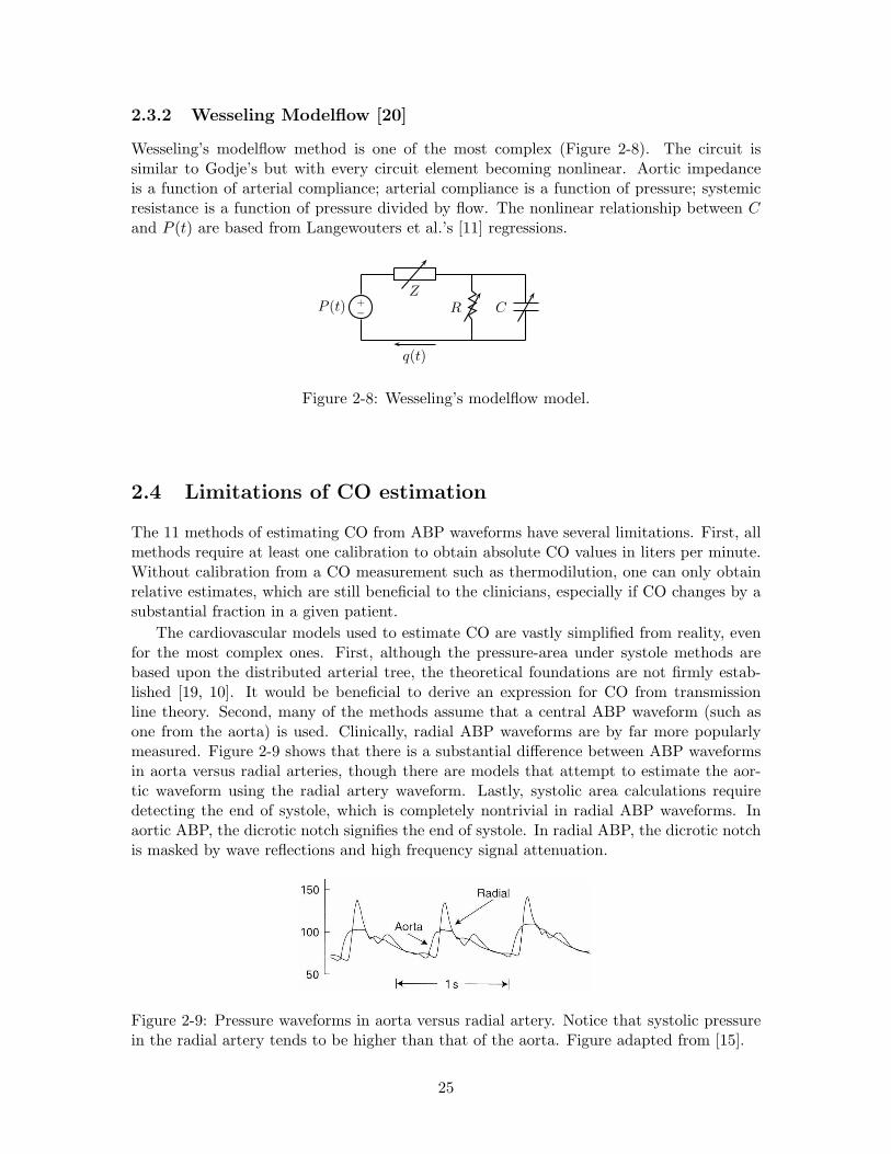
2.3.2 Wesseling Modelflow [20]
Wesseling’s modelflow method is one of the most complex (Figure 2-8). The circuit issimilar to Godje’s but with every circuit element becoming nonlinear. Aortic impedanceis a function of arterial compliance; arterial compliance is a function of pressure; systemicresistance is a function of pressure divided by flow. The nonlinear relationship between Cand P (t) are based from Langewouters et al.’s [11] regressions.
q(t)
ZP (t) +
−
R C
Figure 2-8: Wesseling’s modelflow model.
2.4 Limitations of CO estimation
The 11 methods of estimating CO from ABP waveforms have several limitations. First, allmethods require at least one calibration to obtain absolute CO values in liters per minute.Without calibration from a CO measurement such as thermodilution, one can only obtainrelative estimates, which are still beneficial to the clinicians, especially if CO changes by asubstantial fraction in a given patient.
The cardiovascular models used to estimate CO are vastly simplified from reality, evenfor the most complex ones. First, although the pressure-area under systole methods arebased upon the distributed arterial tree, the theoretical foundations are not firmly estab-lished [19, 10]. It would be beneficial to derive an expression for CO from transmissionline theory. Second, many of the methods assume that a central ABP waveform (such asone from the aorta) is used. Clinically, radial ABP waveforms are by far more popularlymeasured. Figure 2-9 shows that there is a substantial difference between ABP waveformsin aorta versus radial arteries, though there are models that attempt to estimate the aor-tic waveform using the radial artery waveform. Lastly, systolic area calculations requiredetecting the end of systole, which is completely nontrivial in radial ABP waveforms. Inaortic ABP, the dicrotic notch signifies the end of systole. In radial ABP, the dicrotic notchis masked by wave reflections and high frequency signal attenuation.
Figure 2-9: Pressure waveforms in aorta versus radial artery. Notice that systolic pressurein the radial artery tends to be higher than that of the aorta. Figure adapted from [15].
25

For several reasons, the more complex methods may perform worse than the simplerones. First, due to corruption susceptibility of the ABP waveform, especially in a clinicalsetting, complex methods may falter if a particular ABP feature is corrupt. The simplestmethod, CO is proportional to mean arterial pressure, is by far most robust to noise becauseof its averaging nature. Second, the more complex methods have more circuit components.Wesseling’s modelflow method determines the value of each component through ABP wave-forms and regressions using age and gender. Regression lines were determined from a verysmall population (less than 50), which may not be representative of the entire human pop-ulation. Therefore, modelflow may only perform well on patients with similar physiologyto Wesseling’s small study population.
A fundamental limitation of CO estimation performance is due to ABP waveform quality.Features and morphology of the ABP waveform need to be clean, especially for the morecomplex CO estimation methods. Thus, CO estimation is likely to fail in patients withintra-aortic balloon pumps, valve regurgitation diseases, and long-lasting arrhythmias suchas atrial fibrillation.
Further discussion on the limitations of CO estimation can be found in an editorial byLieshout and Wesseling [18].
26
Chapter 3
Signal Abnormality Indexing
3.1 Introduction
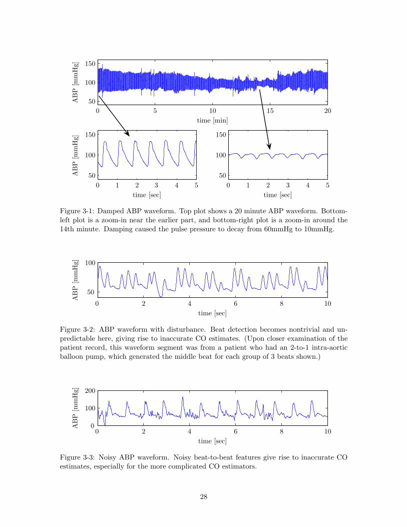
Cardiac output (CO) estimation from arterial blood pressure (ABP) waveforms rely ona clean ABP waveform, in which beat-to-beat features such as mean pressure, duration ofsystole, and beat period may be reliably obtained. Noisy, artifactual, damped, and irregular(not sinus rhythm) ABP waveforms may easily lead to bizarre CO estimates. Figures 3-1, 3-2, 3-3, 3-4 show examples of clinical ABP waveforms from MIMIC II in which CO estimatesare likely to fail. Therefore, it is important to design an algorithm that can flag anomalousbeats in the ABP waveform (Figure 3-4). We define a beat as anomalous when any featurein the beat becomes obscured. Median filtering helps to reduce some sporadic anomalies,but fails as anomalies become more frequent.
In this chapter, we present the signal abnormality index (SAI). The algorithm outputsat a beat-level time resolution and intelligently detects abnormal beats by imposing a seriesof constraints on physiologic, noise/artifact, and beat-to-beat variability. SAI does notdistinguish between anomalies arising from physiologic disturbances such as an arrhythmiaand non-physiologic phenomena such as noise.
The SAI algorithm was evaluated on clinical ABP waveforms of 120 patients fromMIMIC II (see Section 1.1.3). Using the 120 records, we quantified the performance ofthe SAI algorithm in 3 ways: comparing the algorithm’s performance to a human expert,analyzing the sensitivity of the algorithm’s output, and determining whether cleaner wave-form segments yield better CO estimates.
3.2 Methods
Figure 3-5 shows an overview of the SAI algorithm. First, a beat detection algorithm [22]marks the onset of each beat. The onset markers allow for feature extraction at beat-levelresolution. For each beat, features such as heart rate, systolic blood pressure, diastolic bloodpressure are obtained. Features are then evaluated by a series of abnormality criteria, whichcheck for noise level, physiologic ranges, and beat-to-beat variations. The output of eachabnormality criterion is binary, ‘0’ for no flag (clean beat) and ‘1’ for flag. Finally, theoutputs of all abnormality criteria are combined via the logical OR operation.
Given an input ABP segment of n beats, the overall output (define as y) is a binary
27
time [min]
AB
P[m
mH
g]
time [sec]
AB
P[m
mH
g]
time [sec]
0 1 2 3 4 50 1 2 3 4 5
0 5 10 15 20
50
100
150
50
100
150
50
100
150
Figure 3-1: Damped ABP waveform. Top plot shows a 20 minute ABP waveform. Bottom-left plot is a zoom-in near the earlier part, and bottom-right plot is a zoom-in around the14th minute. Damping caused the pulse pressure to decay from 60mmHg to 10mmHg.
time [sec]
AB
P[m
mH
g]
0 2 4 6 8 10
50
100
Figure 3-2: ABP waveform with disturbance. Beat detection becomes nontrivial and un-predictable here, giving rise to inaccurate CO estimates. (Upon closer examination of thepatient record, this waveform segment was from a patient who had an 2-to-1 intra-aorticballoon pump, which generated the middle beat for each group of 3 beats shown.)
time [sec]
AB
P[m
mH
g]
0 2 4 6 8 100
100
200
Figure 3-3: Noisy ABP waveform. Noisy beat-to-beat features give rise to inaccurate COestimates, especially for the more complicated CO estimators.
28

time [seconds]
AB
P[m
mH
g]
0 5 10 15 20 250
50
100
150
Figure 3-4: ABP waveform with artifacts. Corruption in the first 15 seconds is likely dueto improper catheterization caused by movement. Corruption in 20-22 seconds is likelya motion artifact. Signal abnormality index (SAI) is shown on bottom, raising a flag inregions of abnormality.
sequence of length n. For the segment, a cumulative SAI (cSAI) is defined as
Y ≡ fraction of flagged beats =1
n
n∑
k=1
y[k]
where y[k] is the SAI of the k-th beat. cSAI, with a continuous domain of 0 ≤ Y ≤ 1, isa useful measure of the abnormality of an entire waveform segment. (e.g. a segment of 50beats with 4 flagged would yield a cSAI of 0.08.)
The rest of this section explains several components of the SAI in detail and proposesmethods for algorithm evaluation.������������������������������
�! "���#�$��%��������� & "���#�$��%��������� ' (�)���$*+ ,,-&&-,,Figure 3-5: SAI block diagram. Input is an ABP waveform. Output is a binary string,assigning a value (no flag=0, flag=1) to each beat in the ABP waveform.
3.2.1 Feature extraction
The feature extraction algorithm obtains a set of features shown in Table 3.1. For eachbeat, Ps and Pd are the local minimum and maximum around the pressure onset point. Pm
is the average pressure between adjacent onsets. T is the time difference between adjacentonsets. Noise level is defined as the average of all negative slopes in each beat.
3.2.2 Abnormality indexing
With blood pressure features available, the SAI algorithm is ready to interpret them. Table3.2 lists the criteria for flagging a beat.
29
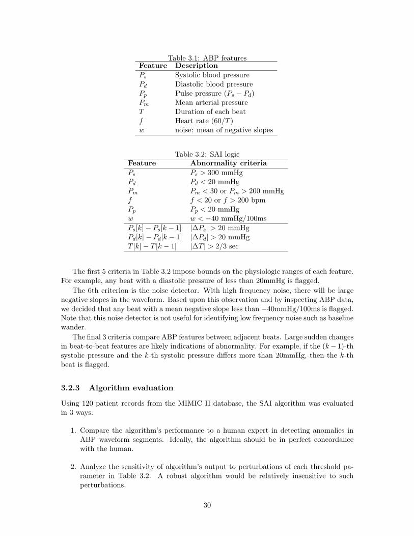
Table 3.1: ABP featuresFeature Description
Ps Systolic blood pressurePd Diastolic blood pressurePp Pulse pressure (Ps − Pd)Pm Mean arterial pressureT Duration of each beatf Heart rate (60/T )w noise: mean of negative slopes
Table 3.2: SAI logicFeature Abnormality criteria
Ps Ps > 300 mmHgPd Pd < 20 mmHgPm Pm < 30 or Pm > 200 mmHgf f < 20 or f > 200 bpmPp Pp < 20 mmHgw w < −40 mmHg/100ms
Ps[k] − Ps[k − 1] |∆Ps| > 20 mmHgPd[k] − Pd[k − 1] |∆Pd| > 20 mmHgT [k] − T [k − 1] |∆T | > 2/3 sec
The first 5 criteria in Table 3.2 impose bounds on the physiologic ranges of each feature.For example, any beat with a diastolic pressure of less than 20mmHg is flagged.
The 6th criterion is the noise detector. With high frequency noise, there will be largenegative slopes in the waveform. Based upon this observation and by inspecting ABP data,we decided that any beat with a mean negative slope less than −40mmHg/100ms is flagged.Note that this noise detector is not useful for identifying low frequency noise such as baselinewander.
The final 3 criteria compare ABP features between adjacent beats. Large sudden changesin beat-to-beat features are likely indications of abnormality. For example, if the (k− 1)-thsystolic pressure and the k-th systolic pressure differs more than 20mmHg, then the k-thbeat is flagged.
3.2.3 Algorithm evaluation
Using 120 patient records from the MIMIC II database, the SAI algorithm was evaluatedin 3 ways:
1. Compare the algorithm’s performance to a human expert in detecting anomalies inABP waveform segments. Ideally, the algorithm should be in perfect concordancewith the human.
2. Analyze the sensitivity of algorithm’s output to perturbations of each threshold pa-rameter in Table 3.2. A robust algorithm would be relatively insensitive to suchperturbations.
30
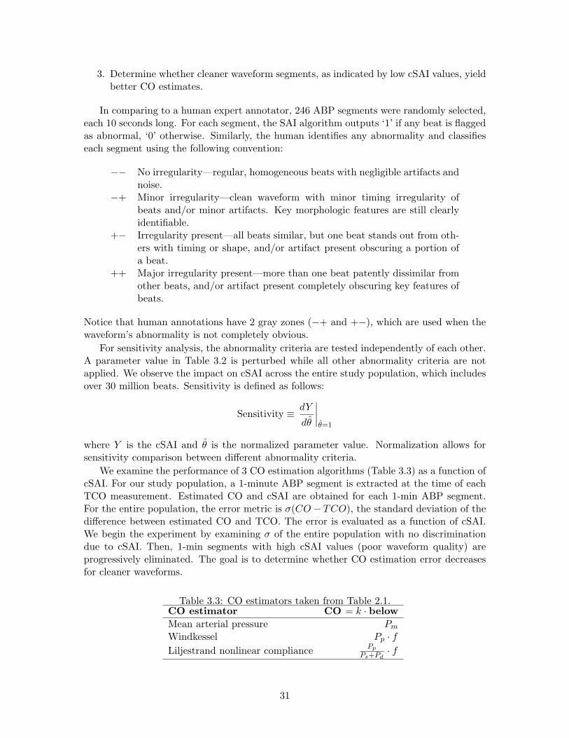
3. Determine whether cleaner waveform segments, as indicated by low cSAI values, yieldbetter CO estimates.
In comparing to a human expert annotator, 246 ABP segments were randomly selected,each 10 seconds long. For each segment, the SAI algorithm outputs ‘1’ if any beat is flaggedas abnormal, ‘0’ otherwise. Similarly, the human identifies any abnormality and classifieseach segment using the following convention:
−− No irregularity—regular, homogeneous beats with negligible artifacts andnoise.
−+ Minor irregularity—clean waveform with minor timing irregularity ofbeats and/or minor artifacts. Key morphologic features are still clearlyidentifiable.
+− Irregularity present—all beats similar, but one beat stands out from oth-ers with timing or shape, and/or artifact present obscuring a portion ofa beat.
++ Major irregularity present—more than one beat patently dissimilar fromother beats, and/or artifact present completely obscuring key features ofbeats.
Notice that human annotations have 2 gray zones (−+ and +−), which are used when thewaveform’s abnormality is not completely obvious.
For sensitivity analysis, the abnormality criteria are tested independently of each other.A parameter value in Table 3.2 is perturbed while all other abnormality criteria are notapplied. We observe the impact on cSAI across the entire study population, which includesover 30 million beats. Sensitivity is defined as follows:
Sensitivity ≡ dY
dθ̂
∣
∣
∣
∣
θ̂=1
where Y is the cSAI and θ̂ is the normalized parameter value. Normalization allows forsensitivity comparison between different abnormality criteria.
We examine the performance of 3 CO estimation algorithms (Table 3.3) as a function ofcSAI. For our study population, a 1-minute ABP segment is extracted at the time of eachTCO measurement. Estimated CO and cSAI are obtained for each 1-min ABP segment.For the entire population, the error metric is σ(CO − TCO), the standard deviation of thedifference between estimated CO and TCO. The error is evaluated as a function of cSAI.We begin the experiment by examining σ of the entire population with no discriminationdue to cSAI. Then, 1-min segments with high cSAI values (poor waveform quality) areprogressively eliminated. The goal is to determine whether CO estimation error decreasesfor cleaner waveforms.
Table 3.3: CO estimators taken from Table 2.1.CO estimator CO = k · below
Mean arterial pressure Pm
Windkessel Pp · fLiljestrand nonlinear compliance
Pp
Ps+Pd· f
31
3.3 Results
3.3.1 SAI versus human
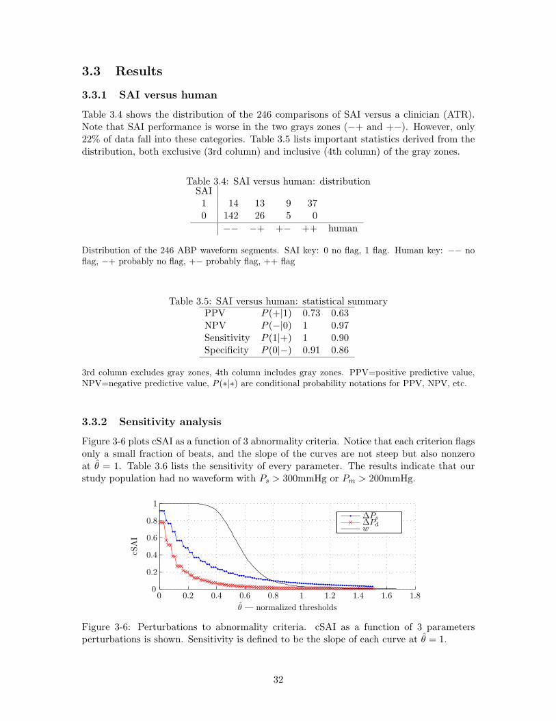
Table 3.4 shows the distribution of the 246 comparisons of SAI versus a clinician (ATR).Note that SAI performance is worse in the two grays zones (−+ and +−). However, only22% of data fall into these categories. Table 3.5 lists important statistics derived from thedistribution, both exclusive (3rd column) and inclusive (4th column) of the gray zones.
Table 3.4: SAI versus human: distributionSAI1 14 13 9 370 142 26 5 0
−− −+ +− ++ human
Distribution of the 246 ABP waveform segments. SAI key: 0 no flag, 1 flag. Human key: −− noflag, −+ probably no flag, +− probably flag, ++ flag
Table 3.5: SAI versus human: statistical summaryPPV P (+|1) 0.73 0.63NPV P (−|0) 1 0.97Sensitivity P (1|+) 1 0.90Specificity P (0|−) 0.91 0.86
3rd column excludes gray zones, 4th column includes gray zones. PPV=positive predictive value,NPV=negative predictive value, P (∗|∗) are conditional probability notations for PPV, NPV, etc.
3.3.2 Sensitivity analysis
Figure 3-6 plots cSAI as a function of 3 abnormality criteria. Notice that each criterion flagsonly a small fraction of beats, and the slope of the curves are not steep but also nonzeroat θ̂ = 1. Table 3.6 lists the sensitivity of every parameter. The results indicate that ourstudy population had no waveform with Ps > 300mmHg or Pm > 200mmHg.
θ̂ — normalized thresholds
cSA
I
∆Ps∆Pdw
0 0.2 0.4 0.6 0.8 1 1.2 1.4 1.6 1.80
0.2
0.4
0.6
0.8
1
Figure 3-6: Perturbations to abnormality criteria. cSAI as a function of 3 parametersperturbations is shown. Sensitivity is defined to be the slope of each curve at θ̂ = 1.
32
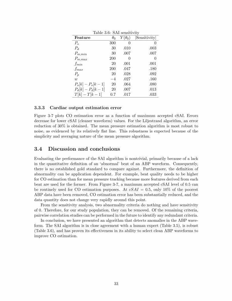
Table 3.6: SAI sensitivityFeature θ0 Y (θ0) |Sensitivity|Ps 300 0 0Pd 30 .010 .003Pm,min 30 .007 .007Pm,max 200 0 0fmin 20 .001 .001fmax 200 .047 .180Pp 20 .028 .092w −4 .027 .160Ps[k] − Ps[k − 1] 20 .064 .080Pd[k] − Pd[k − 1] 20 .007 .013T [k] − T [k − 1] 0.7 .017 .033
3.3.3 Cardiac output estimation error
Figure 3-7 plots CO estimation error as a function of maximum accepted cSAI. Errorsdecrease for lower cSAI (cleaner waveform) values. For the Liljestrand algorithm, an errorreduction of 30% is obtained. The mean pressure estimation algorithm is most robust tonoise, as evidenced by its relatively flat line. This robustness is expected because of thesimplicity and averaging nature of the mean pressure algorithm.
3.4 Discussion and conclusions
Evaluating the performance of the SAI algorithm is nontrivial, primarily because of a lackin the quantitative definition of an ‘abnormal’ beat of an ABP waveform. Consequently,there is no established gold standard to compare against. Furthermore, the definition ofabnormality can be application dependent. For example, beat quality needs to be higherfor CO estimation than for mean pressure tracking because more features derived from eachbeat are used for the former. From Figure 3-7, a maximum accepted cSAI level of 0.5 canbe routinely used for CO estimation purposes. At cSAI = 0.5, only 10% of the poorestABP data have been removed, CO estimation error has been substantially reduced, and thedata quantity does not change very rapidly around this point.
From the sensitivity analysis, two abnormality criteria do nothing and have sensitivityof 0. Therefore, for our study population, they can be removed. Of the remaining criteria,pairwise correlation studies can be performed in the future to identify any redundant criteria.
In conclusion, we have presented an algorithm that detects anomalies in the ABP wave-form. The SAI algorithm is in close agreement with a human expert (Table 3.5), is robust(Table 3.6), and has proven its effectiveness in its ability to select clean ABP waveforms toimprove CO estimation.
33

Cardiac output estimation error
erro
r[L
/min
]
Mean pressureWindkesselLiljestrand
nor
mal
ized
dat
aquan
tity
maximum accepted cSAI
0 0.1 0.2 0.3 0.4 0.5 0.6 0.7 0.8 0.9 1
0 0.1 0.2 0.3 0.4 0.5 0.6 0.7 0.8 0.9 1
0.4
0.5
0.6
0.7
0.8
0.9
1
0.6
0.7
0.8
0.9
1
1.1
Figure 3-7: CO estimation error as a function of maximum accepted cSAI. Bottom plotshows that the amount of data also decreases as we restrict ourselves to cleaner waveforms.
34
Chapter 4
Evaluation Methods
Evaluating the performance of cardiac output (CO) estimation requires obtaining the fol-lowing signals:
• A set of ABP waveforms as input for the CO estimators. In order to capture theintra-beat waveform morphology, sampling rate of ABP needs to be sufficiently high(greater than 60Hz).
• A set of gold-standard CO measurements to compare with estimated CO. Eachmeasurement must be available simultaneously to ABP waveform recordings. We willuse thermodilution CO (TCO) measurements as gold-standard. It is well known thatTCO has errors itself [17]. Thus, by comparing estimated CO to TCO, our resultsare limited by TCO’s accuracy.
The signals will be processed by the following systems:
• A data extraction system to identify suitable ABP waveforms and TCO measure-ments for analysis.
• A CO estimation system to accurately and efficiently implement each CO estima-tion algorithm. Ideally, we obtain the 11 algorithms from the original creators anduse their exact implementation. However, this is impractical in many ways. Hence,we peruse their publications and mimic their methods as closely as possible.
• A comparison system to output the error between each estimated CO and TCO.This system may seem trivial, involving a simple subtraction. However, a majorproblem is that all CO estimates are given in relative units (Table 2.1). Therefore,we must establish suitable calibration methods before performing comparisons. Wealso design a scheme comparing percentage changes in estimated CO and TCO. Thisscheme does not require calibration.
• An error analysis system to report the performance of CO estimates across theentire study population. We also explore the physiologic conditions in which COestimators are likely to fail. Using these analyses, our goals are (1) to determinewhether CO estimates are reliable enough for clinical use, and (2) to investigate thepossibility of improving CO estimates.
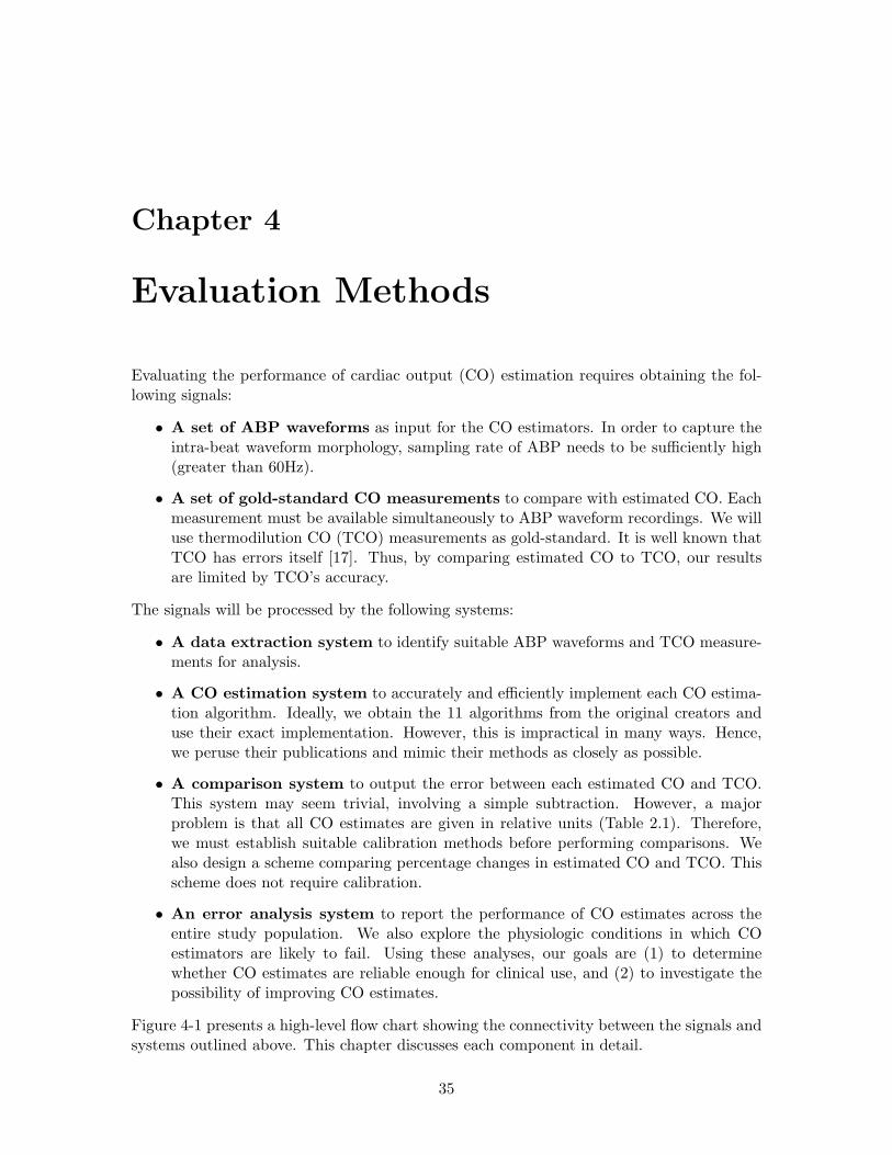
Figure 4-1 presents a high-level flow chart showing the connectivity between the signals andsystems outlined above. This chapter discusses each component in detail.
35
./01023/43536378 9:;<353 8=5>3250?1 9:@.3>4032 ?A5BA58750C350?1DEF 9:G.?CB3>07?1 9:9H>>?> 313/I707J?/4K753143>4 .L8750C3584 .L 8>>?>Figure 4-1: A system for evaluating CO estimation performance.
4.1 Data extraction
Relevant source code: wavex.m, trendex.m 1
As described in Chapter 1, the clinical database we use is MIMIC II, which contains phys-iologic waveform data from over 3500 ICU patients hospitalized at Beth Israel DeaconessMedical Center, Boston, USA. From this database, we identified 120 patients with simul-taneously available ABP waveforms and TCO measurements. The ABP waveforms aremeasured radially and stored as 8-bit quantized data with a temporal resolution of 125Hz.TCO is measured intermittently with a temporal resolution of 1 minute.
4.2 Implementation of CO estimators
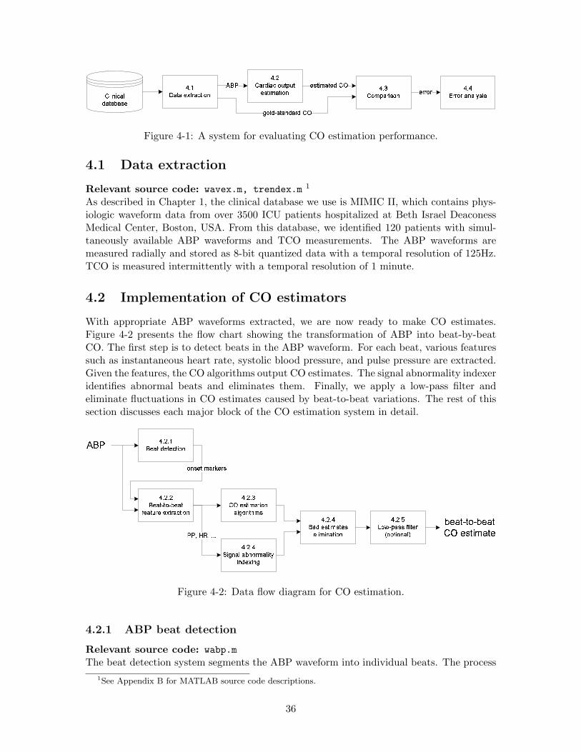
With appropriate ABP waveforms extracted, we are now ready to make CO estimates.Figure 4-2 presents the flow chart showing the transformation of ABP into beat-by-beatCO. The first step is to detect beats in the ABP waveform. For each beat, various featuressuch as instantaneous heart rate, systolic blood pressure, and pulse pressure are extracted.Given the features, the CO algorithms output CO estimates. The signal abnormality indexeridentifies abnormal beats and eliminates them. Finally, we apply a low-pass filter andeliminate fluctuations in CO estimates caused by beat-to-beat variations. The rest of thissection discusses each major block of the CO estimation system in detail.MNONPQRST URTRVTWXY MNONZ[\ R]TW^STWXYS_`XaWTb^]MNONMcW`YS_ SdYXa^S_WTeWYURfWY` MNONghXijkS]] lW_TRamXkTWXYS_n
XY]RT ^SaoRa]MNONOQRSTjTXjdRSTlRSTpaR RfTaSVTWXYqqr str NNN MNONMQSU R]TW^STR]R_W^WYSTWXYuvw
xyz{|{}|xyz{~� y�{��z{yFigure 4-2: Data flow diagram for CO estimation.
4.2.1 ABP beat detection
Relevant source code: wabp.m
The beat detection system segments the ABP waveform into individual beats. The process
1See Appendix B for MATLAB source code descriptions.
36
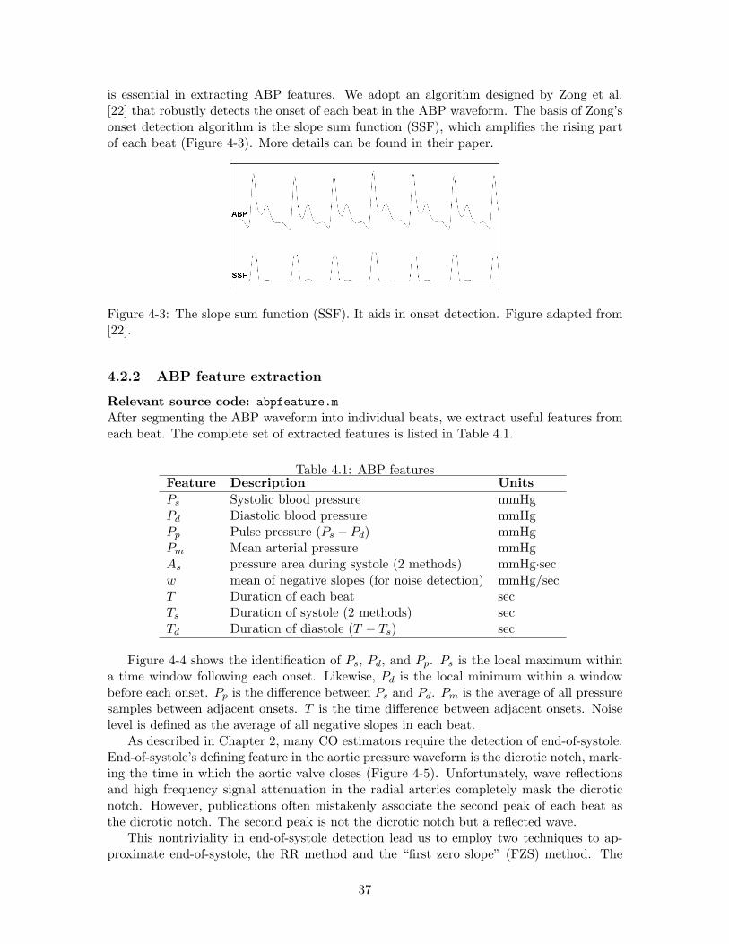
is essential in extracting ABP features. We adopt an algorithm designed by Zong et al.[22] that robustly detects the onset of each beat in the ABP waveform. The basis of Zong’sonset detection algorithm is the slope sum function (SSF), which amplifies the rising partof each beat (Figure 4-3). More details can be found in their paper.
Figure 4-3: The slope sum function (SSF). It aids in onset detection. Figure adapted from[22].
4.2.2 ABP feature extraction
Relevant source code: abpfeature.m
After segmenting the ABP waveform into individual beats, we extract useful features fromeach beat. The complete set of extracted features is listed in Table 4.1.
Table 4.1: ABP featuresFeature Description Units
Ps Systolic blood pressure mmHgPd Diastolic blood pressure mmHgPp Pulse pressure (Ps − Pd) mmHgPm Mean arterial pressure mmHgAs pressure area during systole (2 methods) mmHg·secw mean of negative slopes (for noise detection) mmHg/secT Duration of each beat secTs Duration of systole (2 methods) secTd Duration of diastole (T − Ts) sec
Figure 4-4 shows the identification of Ps, Pd, and Pp. Ps is the local maximum withina time window following each onset. Likewise, Pd is the local minimum within a windowbefore each onset. Pp is the difference between Ps and Pd. Pm is the average of all pressuresamples between adjacent onsets. T is the time difference between adjacent onsets. Noiselevel is defined as the average of all negative slopes in each beat.
As described in Chapter 2, many CO estimators require the detection of end-of-systole.End-of-systole’s defining feature in the aortic pressure waveform is the dicrotic notch, mark-ing the time in which the aortic valve closes (Figure 4-5). Unfortunately, wave reflectionsand high frequency signal attenuation in the radial arteries completely mask the dicroticnotch. However, publications often mistakenly associate the second peak of each beat asthe dicrotic notch. The second peak is not the dicrotic notch but a reflected wave.
This nontriviality in end-of-systole detection lead us to employ two techniques to ap-proximate end-of-systole, the RR method and the “first zero slope” (FZS) method. The
37

time [seconds]
AB
P[m
mH
g]
-0.4 -0.2 0 0.2 0.4 0.6
50
60
70
80
90
Figure 4-4: Ps, Pd, and Pp detection. The light dot marks the onset. The darker dots arePs and Pd. The line segment marks Pp. The shaded areas are the two search windows forPs and Pd.
RR method uses a result from electrocardiography. QT-interval duration is approximatedas 0.3
√RR interval [1], where RR-interval is measured in seconds. Intuitively, the QT frac-
tion becomes smaller as the duration of a cardiac cycle lengthens. We approximate thatthe RR-interval equals the beat period. The QT-interval is the duration from electricaldepolarization to repolarization of the ventricles. Therefore, for a normal healthy heart, weapproximate the QT-interval and systolic ABP duration to be very similar. From Figure4-5, these approximations are reasonable. Hence, Ts = 0.3
√T . For the FZS method, we find
the first time following Ps that the slope of ABP becomes 0. Preliminary testing showedthat while the 2 methods may indicate significantly different end-of-systole times (Figure4-6), both offered very similar results in terms of CO estimation performance.
The main purpose for end-of-systole detection is in calculating the area under ABPduring systole of each beat. Figure 4-6 shows end-of-systole and systolic area.
As =
∫
Ts
(P (t) − Pd)dt
4.2.3 CO estimator implementation
Relevant source code: est0<num> <title>.m
The first 9 CO estimators in Table 2.1 take features of the ABP waveform as input. Simplearithmetic operations are applied to produce beat-to-beat CO estimates. The last 2 esti-mators use beat-to-beat features and the raw ABP waveform. Differential equations areused to produce a flow waveform. Then, we integrate the flow waveform over the systolicduration to produce CO estimates.
4.2.4 Signal quality and bad beats elimination
Relevant source code: jSQI.m, estimateCO.m
Quality of the ABP waveform is essential in determining the performance of CO estimators.Noisy, artifactual, damped, and irregular (not sinus rhythm) ABP waveforms may easilylead to bizarre CO estimates. Figures 3-1, 3-4, 3-2, 3-3 from Chapter 3 show examples ofABP waveforms from MIMIC II in which CO estimates are likely to fail. In Chapter 3, wepresented the SAI algorithm to flag abnormal beats in the ABP waveform. Flagged beats
38
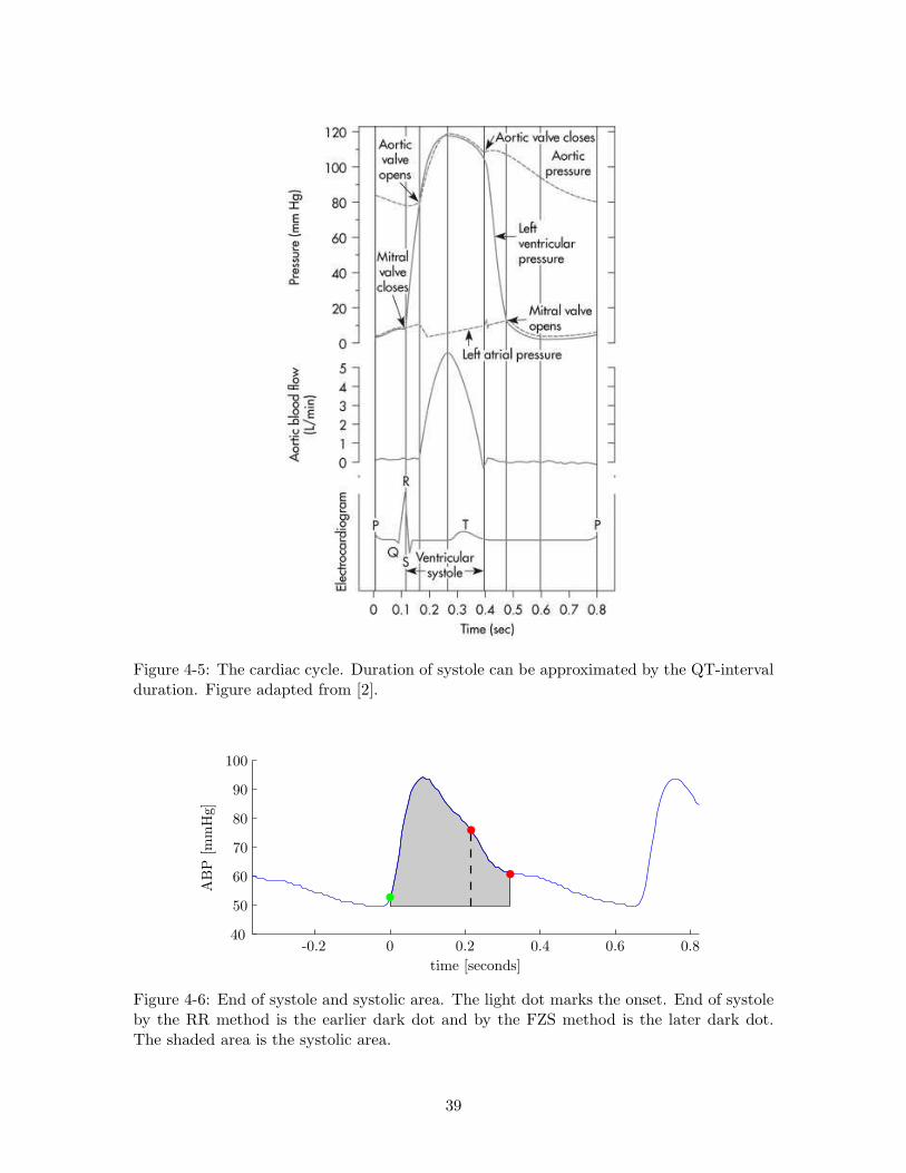
Figure 4-5: The cardiac cycle. Duration of systole can be approximated by the QT-intervalduration. Figure adapted from [2].
time [seconds]
AB
P[m
mH
g]
-0.2 0 0.2 0.4 0.6 0.840
50
60
70
80
90
100
Figure 4-6: End of systole and systolic area. The light dot marks the onset. End of systoleby the RR method is the earlier dark dot and by the FZS method is the later dark dot.The shaded area is the systolic area.
39
do not participate in CO estimation. Also, if a substantial percentage of beats are flaggedin a given segment, the entire segment is excluded from CO estimation.
4.2.5 Running-average LPF to reduce beat-to-beat fluctuations
Relevant source code: estimateCO.m
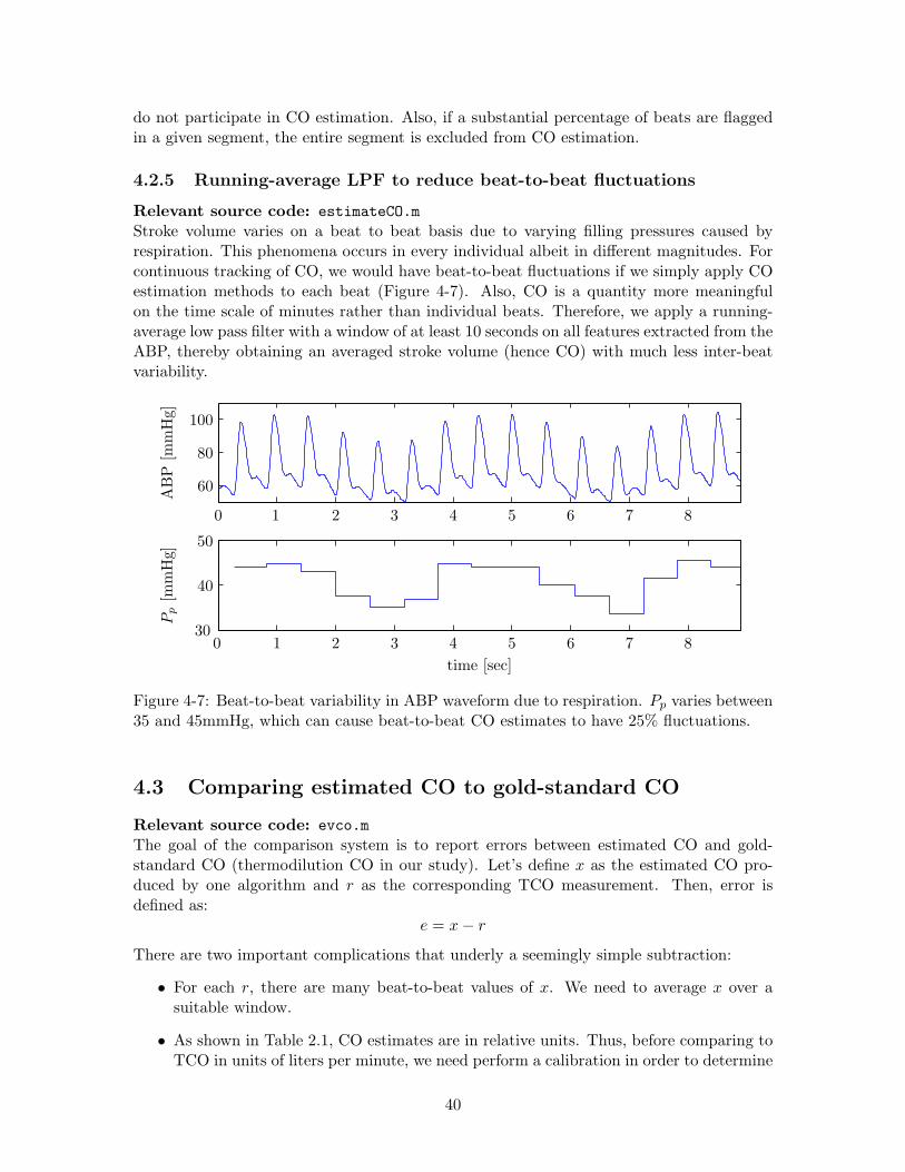
Stroke volume varies on a beat to beat basis due to varying filling pressures caused byrespiration. This phenomena occurs in every individual albeit in different magnitudes. Forcontinuous tracking of CO, we would have beat-to-beat fluctuations if we simply apply COestimation methods to each beat (Figure 4-7). Also, CO is a quantity more meaningfulon the time scale of minutes rather than individual beats. Therefore, we apply a running-average low pass filter with a window of at least 10 seconds on all features extracted from theABP, thereby obtaining an averaged stroke volume (hence CO) with much less inter-beatvariability.
AB
P[m
mH
g]
time [sec]
Pp
[mm
Hg]
0 1 2 3 4 5 6 7 8
0 1 2 3 4 5 6 7 8
30
40
50
60
80
100
Figure 4-7: Beat-to-beat variability in ABP waveform due to respiration. Pp varies between35 and 45mmHg, which can cause beat-to-beat CO estimates to have 25% fluctuations.
4.3 Comparing estimated CO to gold-standard CO
Relevant source code: evco.m
The goal of the comparison system is to report errors between estimated CO and gold-standard CO (thermodilution CO in our study). Let’s define x as the estimated CO pro-duced by one algorithm and r as the corresponding TCO measurement. Then, error isdefined as:
e = x − r
There are two important complications that underly a seemingly simple subtraction:
• For each r, there are many beat-to-beat values of x. We need to average x over asuitable window.
• As shown in Table 2.1, CO estimates are in relative units. Thus, before comparing toTCO in units of liters per minute, we need perform a calibration in order to determine
40
the proportionality constant k.
Large percentage rises or drops in CO are of clinical interest. We devise a method to reportthe accuracy of CO estimates in determining percentage changes without calibration.
4.3.1 Averaging beat-to-beat CO estimates
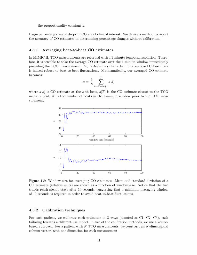
In MIMIC II, TCO measurements are recorded with a 1-minute temporal resolution. There-fore, it is sensible to take the average CO estimate over the 1-minute window immediatelypreceding the TCO measurement. Figure 4-8 shows that a 1-minute averaged CO estimateis indeed robust to beat-to-beat fluctuations. Mathematically, our averaged CO estimatebecomes:
x =1
N
T∑
k=T−N+1
a[k]
where a[k] is CO estimate at the k-th beat, a[T ] is the CO estimate closest to the TCOmeasurement, N is the number of beats in the 1-minute window prior to the TCO mea-surement.
µ
window size [seconds]
σ
0 20 40 60 80 100
0 20 40 60 80 100
7
8
9
10
11
24
26
28
30
32
Figure 4-8: Window size for averaging CO estimates. Mean and standard deviation of aCO estimate (relative units) are shown as a function of window size. Notice that the twotrends reach steady state after 10 seconds, suggesting that a minimum averaging windowof 10 seconds is required in order to avoid beat-to-beat fluctuations.
4.3.2 Calibration techniques
For each patient, we calibrate each estimator in 3 ways (denoted as C1, C2, C3), eachtailoring towards a different use model. In two of the calibration methods, we use a vector-based approach. For a patient with N TCO measurements, we construct an N -dimensionalcolumn vector, with one dimension for each measurement:
41
Reference CO (TCO): r =[
r1 r2 · · · rN
]
′
Uncalibrated estimate: x =[
x1 x2 · · · xN
]
′
Calibrated estimate: q = kx
r
xkx
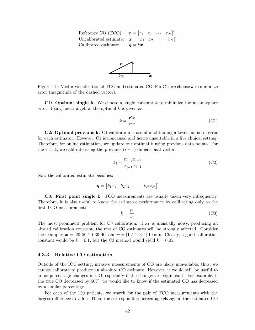
Figure 4-9: Vector visualization of TCO and estimated CO. For C1, we choose k to minimizeerror (magnitude of the dashed vector).
C1: Optimal single k. We choose a single constant k to minimize the mean squareerror. Using linear algebra, the optimal k is given as:
k =r′x
x′x(C1)
C2: Optimal previous k. C1 calibration is useful in obtaining a lower bound of errorfor each estimator. However, C1 is noncausal and hence unsuitable in a live clinical setting.Therefore, for online estimation, we update our optimal k using previous data points. Forthe i-th k, we calibrate using the previous (i − 1)-dimensional vector:
ki =r′
i−1xi−1
x′
i−1xi−1(C2)
Now the calibrated estimate becomes:
q =[
k1x1 k2x2 · · · kNxN
]
′
C3: First point single k. TCO measurements are usually taken very infrequently.Therefore, it is also useful to know the estimator performance by calibrating only to thefirst TCO measurement:
k =r1
x1(C3)
The most prominent problem for C3 calibration: if x1 is unusually noisy, producing anabsurd calibration constant, the rest of CO estimates will be strongly affected. Considerthe example: x = [20 50 20 30 40] and r = [1 5 2 3 4] L/min. Clearly, a good calibrationconstant would be k = 0.1, but the C3 method would yield k = 0.05.
4.3.3 Relative CO estimation
Outside of the ICU setting, invasive measurements of CO are likely unavailable; thus, wecannot calibrate to produce an absolute CO estimate. However, it would still be useful toknow percentage changes in CO, especially if the changes are significant. For example, ifthe true CO decreased by 50%, we would like to know if the estimated CO has decreasedby a similar percentage.
For each of the 120 patients, we search for the pair of TCO measurements with thelargest difference in value. Then, the corresponding percentage change in the estimated CO
42

(∆x) and TCO (∆r) are compared. Mathematically:
∆r =
(
r[imax]r[imin] − 1
)
× 100 if t[imax] > t[imin](
r[imin]r[imax] − 1
)
× 100 if t[imax] < t[imin]
∆x =
(
x[imax]x[imin] − 1
)
× 100 if t[imax] > t[imin](
x[imin]x[imax] − 1
)
× 100 if t[imax] < t[imin]
where imax is the index in which maximum TCO occurs, and correspondingly for imin.
4.4 Error analysis
In the previous section, we established methods to obtain the error between each TCOmeasurement and estimated CO. Across the entire study population, for each CO estimator,we have an error distribution. In clinical literature, the most popular representation of errordistributions is the Bland-Altman plot [3]. Figure 4-10 shows an example. The horizontalaxis is the average of TCO and estimated CO. The vertical axis is the error. The majoradvantage of such a plot is that it enables one to see whether there’s any correlation betweenthe error and the averaged CO. For example, if error becomes substantial for high CO, thenthe estimated CO should not be trusted whenever it gives a high CO value.
x−
r[L
/min
]
(x + r)/2 [L/min]
CO estimator: Liljestrand & Zander
0 2 4 6 8 10 12-6
-4
-2
0
2
4
6
Figure 4-10: A sample Bland-Altman plot. The error histogram is shown on the left. Thesolid lines show 1 SD bounds, and the dashed lines show 95% confidence intervals.
With the aid of Bland-Altman plots, we present the performance of each CO estimator inthe following ways:
CO estimation error. We report the 1SD and 95% confidence interval of the error dis-tribution. If the error distribution is Gaussian, the numerical values for the 95% confidenceinterval and 2SD coincide.
k-variability. A good CO estimator should have a calibration constant (k) with low
43
variability across different patients. For example, if one ideal CO estimator has k = 5±0.01for all of the 120 patients, then we can assume k = 5 and obtain the absolute CO estimatefor any patient. However, if k = 5 ± 5, then calibration is necessary for each patient.Mathematically, we quantify k-variability as:
k-variability =SD of k for the study population
mean of k for the study population=
σ(k)
µ(k)
Division by µ(k) enables us to compare the variability of k among different CO estimators.A k-variability of 0.1 would mean that the k fluctuates by 10% around the mean.
CO-variability. A good CO estimator should produce beat-to-beat CO estimates withvariability on the order of stroke volume and heart rate variability. It is undesirable forthe stroke volumes to fluctuate beyond physiologically plausible ranges from beat-to-beat.CO-variability is measured for each 1-minute ABP waveform in which we obtain beat-to-beat CO estimates (no LPF is applied here). We assume that the physiological state isstable (e.g. average CO is constant) over the 1-minute window. Similar to k-variability,CO-variability is defined mathematically as:
CO-variability =SD of CO for a 1-min ABP waveform
mean of CO for a 1-min ABP waveform=
σ(q)
µ(q)
For each CO estimator, we report the average CO-variability over the entire study popu-lation. Because of the division by µ(CO), calibration is not necessary to determine CO-variability.
Relative CO estimation error. A good CO estimator, when uncalibrated, shouldstill agree with TCO in terms of percentage increases and decreases. As discussed in Section4.3.3, for each patient we identify the pair of data points with most significant change inTCO and compare it to the corresponding estimated CO. Figure 4-11 shows an exampleof relative CO estimation performance. For each CO estimator, we report the 1SD of theerror distribution between percentage changes in estimated CO and TCO. We also reportthe performance of detecting directional changes, defined as:
P (+|+) = probability of an increase in estimated CO given an increase in TCO
P (−|−) = probability of an decrease in estimated CO given an decrease in TCO
Subset error analysis. A CO estimator may perform better in certain physiologicconditions than others. In subset error analysis, we show interesting plots of CO estimationerror as a function of ABP features such as heart rate and mean arterial pressure. Forexample, a possible discovery would be that one CO estimator performs worse in high heartrates than low heart rates.
44

TCO percentage change
esti
mat
edC
Oper
centa
gech
ange
-100 -50 0 50 100 150 200-100
-50
0
50
100
150
200
Figure 4-11: Percentage changes in TCO versus estimated CO. Ideally, every point lies onthe diagonal line. A point that lies in one of the two shaded zones means that the estimatedCO and TCO agree in terms of directional (increase/decrease) change.
45

46
Chapter 5
Results and Discussion
5.1 Subject population statistics
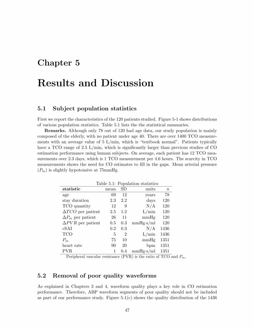
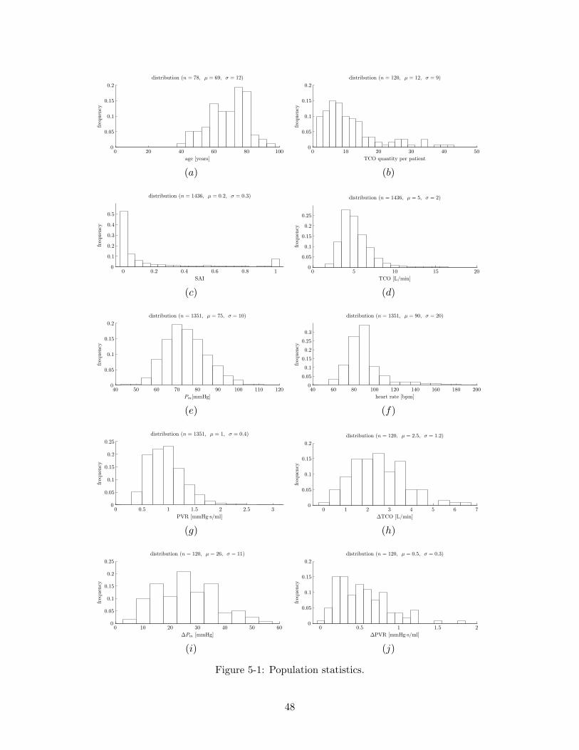
First we report the characteristics of the 120 patients studied. Figure 5-1 shows distributionsof various population statistics. Table 5.1 lists the the statistical summaries.
Remarks. Although only 78 out of 120 had age data, our study population is mainlycomposed of the elderly, with no patient under age 40. There are over 1400 TCO measure-ments with an average value of 5 L/min, which is “textbook normal”. Patients typicallyhave a TCO range of 2.5 L/min, which is significantly larger than previous studies of COestimation performance using human subjects. On average, each patient has 12 TCO mea-surements over 2.3 days, which is 1 TCO measurement per 4.6 hours. The scarcity in TCOmeasurements shows the need for CO estimates to fill in the gaps. Mean arterial pressure(Pm) is slightly hypotensive at 75mmHg.
Table 5.1: Population statisticsstatistic mean SD units n
age 69 12 years 78stay duration 2.3 2.2 days 120TCO quantity 12 9 N/A 120∆TCO per patient 2.5 1.2 L/min 120∆Pm per patient 26 11 mmHg 120∆PV R per patient 0.5 0.3 mmHg·s/ml 120cSAI 0.2 0.3 N/A 1436TCO 5 2 L/min 1436Pm 75 10 mmHg 1351heart rate 90 20 bpm 1351PVR 1 0.4 mmHg·s/ml 1351
Peripheral vascular resistance (PVR) is the ratio of TCO and Pm.
5.2 Removal of poor quality waveforms
As explained in Chapters 3 and 4, waveform quality plays a key role in CO estimationperformance. Therefore, ABP waveform segments of poor quality should not be includedas part of our performance study. Figure 5-1(c) shows the quality distribution of the 1436
47
age [years]
freq
uen
cy
distribution (n = 78, µ = 69, σ = 12)
0 20 40 60 80 1000
0.05
0.1
0.15
0.2
TCO quantity per patient
freq
uen
cy
distribution (n = 120, µ = 12, σ = 9)
0 10 20 30 40 500
0.05
0.1
0.15
0.2
(a) (b)
SAI
freq
uen
cy
distribution (n = 1436, µ = 0.2, σ = 0.3)
0 0.2 0.4 0.6 0.8 10
0.1
0.2
0.3
0.4
0.5
TCO [L/min]
freq
uen
cy
distribution (n = 1436, µ = 5, σ = 2)
0 5 10 15 200
0.05
0.1
0.15
0.2
0.25
(c) (d)
Pm[mmHg]
freq
uen
cy
distribution (n = 1351, µ = 75, σ = 10)
40 50 60 70 80 90 100 110 1200
0.05
0.1
0.15
0.2
heart rate [bpm]
freq
uen
cy
distribution (n = 1351, µ = 90, σ = 20)
40 60 80 100 120 140 160 180 2000
0.05
0.1
0.15
0.2
0.25
0.3
(e) (f)
PVR [mmHg·s/ml]
freq
uen
cy
distribution (n = 1351, µ = 1, σ = 0.4)
0 0.5 1 1.5 2 2.5 30
0.05
0.1
0.15
0.2
0.25
∆TCO [L/min]
freq
uen
cy
distribution (n = 120, µ = 2.5, σ = 1.2)
0 1 2 3 4 5 6 70
0.05
0.1
0.15
0.2
(g) (h)
∆Pm [mmHg]
freq
uen
cy
distribution (n = 120, µ = 26, σ = 11)
0 10 20 30 40 50 600
0.05
0.1
0.15
0.2
0.25
∆PVR [mmHg·s/ml]
freq
uen
cy
distribution (n = 120, µ = 0.5, σ = 0.3)
0 0.5 1 1.5 20
0.05
0.1
0.15
0.2
(i) (j)
Figure 5-1: Population statistics.
48
1-min ABP waveforms segments using the cSAI metric. For cSAI, “0” is clean and “1” iscompletely poor. The majority of waveforms are clean. Based upon this distribution andresults shown in Figure 3-7, we decided to only use waveform segments with cSAI < 0.4for our analyses. Figure 5-2 shows the Bland-Altman plot of the Liljestrand algorithm withdifferent levels of signal quality: In (a), all segments are used. In (b), only waveforms withcSAI < 0.4 are used. In (c), only the pristine (cSAI = 0) waveforms are used. Noticeeven in (a), the number of comparisons is 1230, not 1436. This is because 120 were usedfor calibration and the remaining 86 had waveforms of so low quality that features couldnot be extracted from them. For the rest of this chapter, we only examine CO estimationperformance on ABP waveforms with cSAI < 0.4.
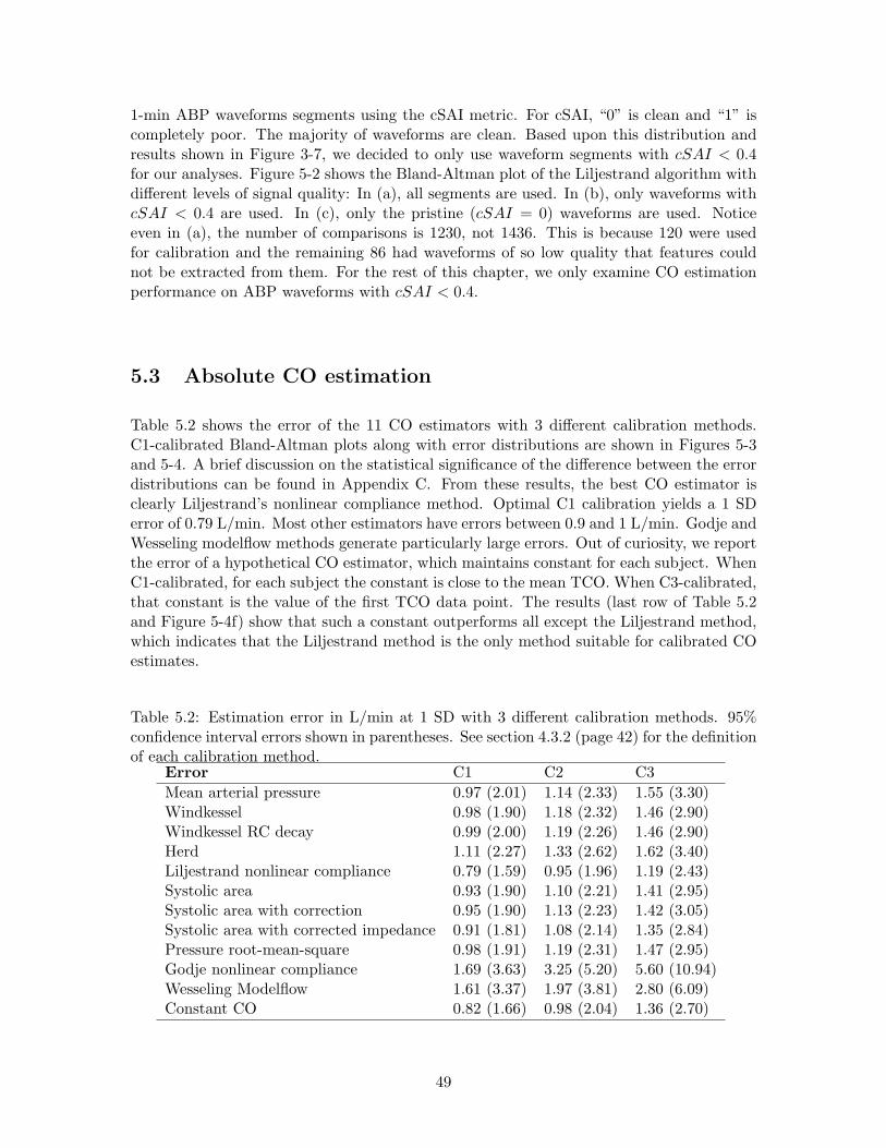
5.3 Absolute CO estimation
Table 5.2 shows the error of the 11 CO estimators with 3 different calibration methods.C1-calibrated Bland-Altman plots along with error distributions are shown in Figures 5-3and 5-4. A brief discussion on the statistical significance of the difference between the errordistributions can be found in Appendix C. From these results, the best CO estimator isclearly Liljestrand’s nonlinear compliance method. Optimal C1 calibration yields a 1 SDerror of 0.79 L/min. Most other estimators have errors between 0.9 and 1 L/min. Godje andWesseling modelflow methods generate particularly large errors. Out of curiosity, we reportthe error of a hypothetical CO estimator, which maintains constant for each subject. WhenC1-calibrated, for each subject the constant is close to the mean TCO. When C3-calibrated,that constant is the value of the first TCO data point. The results (last row of Table 5.2and Figure 5-4f) show that such a constant outperforms all except the Liljestrand method,which indicates that the Liljestrand method is the only method suitable for calibrated COestimates.
Table 5.2: Estimation error in L/min at 1 SD with 3 different calibration methods. 95%confidence interval errors shown in parentheses. See section 4.3.2 (page 42) for the definitionof each calibration method.
Error C1 C2 C3
Mean arterial pressure 0.97 (2.01) 1.14 (2.33) 1.55 (3.30)Windkessel 0.98 (1.90) 1.18 (2.32) 1.46 (2.90)Windkessel RC decay 0.99 (2.00) 1.19 (2.26) 1.46 (2.90)Herd 1.11 (2.27) 1.33 (2.62) 1.62 (3.40)Liljestrand nonlinear compliance 0.79 (1.59) 0.95 (1.96) 1.19 (2.43)Systolic area 0.93 (1.90) 1.10 (2.21) 1.41 (2.95)Systolic area with correction 0.95 (1.90) 1.13 (2.23) 1.42 (3.05)Systolic area with corrected impedance 0.91 (1.81) 1.08 (2.14) 1.35 (2.84)Pressure root-mean-square 0.98 (1.91) 1.19 (2.31) 1.47 (2.95)Godje nonlinear compliance 1.69 (3.63) 3.25 (5.20) 5.60 (10.94)Wesseling Modelflow 1.61 (3.37) 1.97 (3.81) 2.80 (6.09)Constant CO 0.82 (1.66) 0.98 (2.04) 1.36 (2.70)
49

(CO + TCO)/2 [L/min]
CO
esti
mat
ion
erro
r[L
/min
]
Bland-Altman plot (n = 1230, µ(error) = −0.11, σ(error) = 0.98)
0 2 4 6 8 10 12 14-8
-6
-4
-2
0
2
4
6
8
(a) all
(CO + TCO)/2 [L/min]
CO
esti
mat
ion
erro
r[L
/min
]
Bland-Altman plot (n = 1062, µ(error) = −0.06, σ(error) = 0.79)
0 2 4 6 8 10 12 14-8
-6
-4
-2
0
2
4
6
8
(b) cSAI < 0.4
(CO + TCO)/2 [L/min]
CO
esti
mat
ion
erro
r[L
/m
in]
Bland-Altman plot (n = 520, µ(error) = −0.02, σ(error) = 0.65)
0 2 4 6 8 10 12 14-8
-6
-4
-2
0
2
4
6
8
(c) cSAI = 0
Figure 5-2: Bland-Altman plots of the Liljestrand CO estimator with various levels of ABPwaveform quality: from all inclusive (a) to only the most pristine data (c).
50
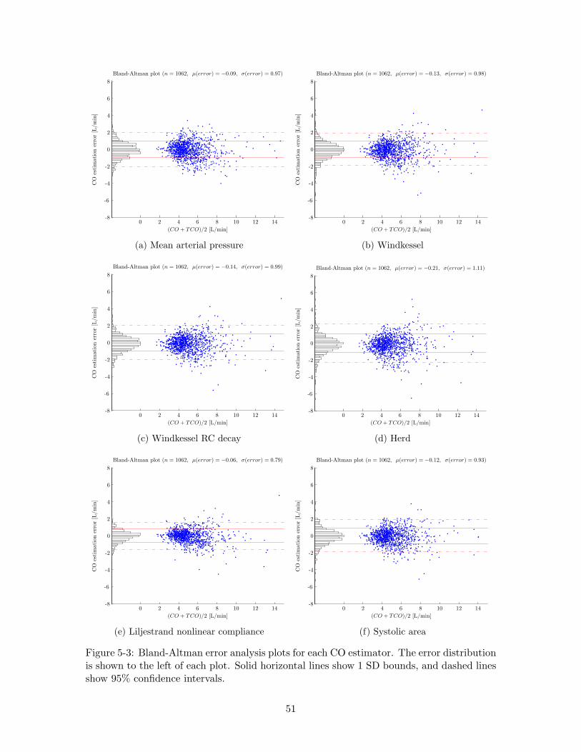
(CO + TCO)/2 [L/min]
CO
esti
mati
on
erro
r[L
/m
in]
Bland-Altman plot (n = 1062, µ(error) = −0.09, σ(error) = 0.97)
0 2 4 6 8 10 12 14-8
-6
-4
-2
0
2
4
6
8
(CO + TCO)/2 [L/min]
CO
esti
mati
on
erro
r[L
/m
in]
Bland-Altman plot (n = 1062, µ(error) = −0.13, σ(error) = 0.98)
0 2 4 6 8 10 12 14-8
-6
-4
-2
0
2
4
6
8
(a) Mean arterial pressure (b) Windkessel
(CO + TCO)/2 [L/min]
CO
esti
mat
ion
erro
r[L
/min
]
Bland-Altman plot (n = 1062, µ(error) = −0.14, σ(error) = 0.99)
0 2 4 6 8 10 12 14-8
-6
-4
-2
0
2
4
6
8
(CO + TCO)/2 [L/min]
CO
esti
mat
ion
erro
r[L
/min
]
Bland-Altman plot (n = 1062, µ(error) = −0.21, σ(error) = 1.11)
0 2 4 6 8 10 12 14-8
-6
-4
-2
0
2
4
6
8
(c) Windkessel RC decay (d) Herd
(CO + TCO)/2 [L/min]
CO
esti
mat
ion
erro
r[L
/min
]
Bland-Altman plot (n = 1062, µ(error) = −0.06, σ(error) = 0.79)
0 2 4 6 8 10 12 14-8
-6
-4
-2
0
2
4
6
8
(CO + TCO)/2 [L/min]
CO
esti
mat
ion
erro
r[L
/min
]
Bland-Altman plot (n = 1062, µ(error) = −0.12, σ(error) = 0.93)
0 2 4 6 8 10 12 14-8
-6
-4
-2
0
2
4
6
8
(e) Liljestrand nonlinear compliance (f) Systolic area
Figure 5-3: Bland-Altman error analysis plots for each CO estimator. The error distributionis shown to the left of each plot. Solid horizontal lines show 1 SD bounds, and dashed linesshow 95% confidence intervals.
51
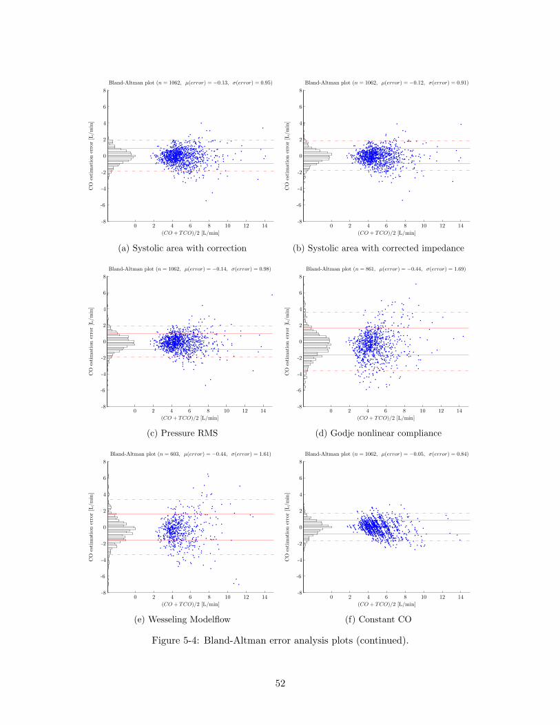
(CO + TCO)/2 [L/min]
CO
esti
mati
on
erro
r[L
/m
in]
Bland-Altman plot (n = 1062, µ(error) = −0.13, σ(error) = 0.95)
0 2 4 6 8 10 12 14-8
-6
-4
-2
0
2
4
6
8
(CO + TCO)/2 [L/min]
CO
esti
mati
on
erro
r[L
/m
in]
Bland-Altman plot (n = 1062, µ(error) = −0.12, σ(error) = 0.91)
0 2 4 6 8 10 12 14-8
-6
-4
-2
0
2
4
6
8
(a) Systolic area with correction (b) Systolic area with corrected impedance
(CO + TCO)/2 [L/min]
CO
esti
mat
ion
erro
r[L
/min
]
Bland-Altman plot (n = 1062, µ(error) = −0.14, σ(error) = 0.98)
0 2 4 6 8 10 12 14-8
-6
-4
-2
0
2
4
6
8
(CO + TCO)/2 [L/min]
CO
esti
mat
ion
erro
r[L
/min
]
Bland-Altman plot (n = 861, µ(error) = −0.44, σ(error) = 1.69)
0 2 4 6 8 10 12 14-8
-6
-4
-2
0
2
4
6
8
(c) Pressure RMS (d) Godje nonlinear compliance
(CO + TCO)/2 [L/min]
CO
esti
mat
ion
erro
r[L
/min
]
Bland-Altman plot (n = 603, µ(error) = −0.44, σ(error) = 1.61)
0 2 4 6 8 10 12 14-8
-6
-4
-2
0
2
4
6
8
(CO + TCO)/2 [L/min]
CO
esti
mat
ion
erro
r[L
/min
]
Bland-Altman plot (n = 1062, µ(error) = −0.05, σ(error) = 0.84)
0 2 4 6 8 10 12 14-8
-6
-4
-2
0
2
4
6
8
(e) Wesseling Modelflow (f) Constant CO
Figure 5-4: Bland-Altman error analysis plots (continued).
52

5.4 Variability of calibration constants
Table 5.3 shows the variability of C1 and C3 calibration constants across the study popu-lation. Liljestrand CO estimator has the lowest C1 and C3 variabilities of 38% and 42%,respectively. These numbers are quite high, indicating that we still must calibrate eachpatient individually in order to obtain absolute CO estimates.
Table 5.3: Variability of k for C1 and C3 calibration.Estimator C1 variability C3 variability
Mean arterial pressure 0.40 0.50Windkessel 0.42 0.48Windkessel RC decay 0.43 0.49Herd 0.47 0.55Liljestrand nonlinear compliance 0.38 0.42Systolic area 0.43 0.48Systolic area with correction 0.44 0.49Systolic area with corrected impedance 0.43 0.48Pressure root-mean-square 0.43 0.48Godje nonlinear compliance 0.62 1.75Wesseling Modelflow 0.42 0.51
5.5 Variability of CO estimates
Table 5.4 shows the average variability of beat-to-beat CO estimates obtained from 1-minute ABP waveforms. The Pm CO estimator has the lowest variability of 4%. The morecomplex estimators have higher variability. These results are plausible because the Pm
estimator takes simple averages of all ABP samples whereas the more complex estimatorsuse individual features from the ABP waveform. We do not have the means to prove whichCO estimation method has variability levels that closest resembles reality. However, a 10%or less variability in stroke volume does seem reasonable.
Table 5.4: Variability of CO estimates.Estimator Variability
Mean arterial pressure 0.04Windkessel 0.09Windkessel RC decay 0.10Herd 0.12Liljestrand nonlinear compliance 0.07Systolic area 0.09Systolic area with correction 0.10Systolic area with corrected impedance 0.10Pressure root-mean-square 0.09Godje nonlinear compliance 0.26Wesseling Modelflow 0.67
53
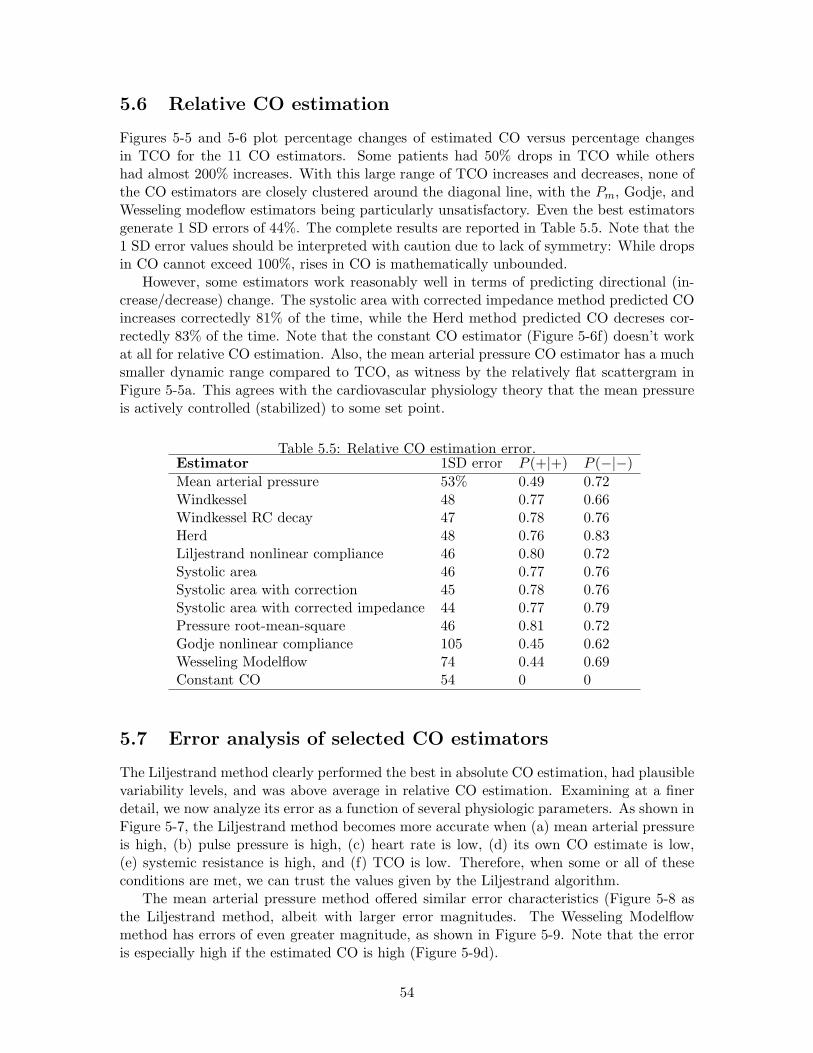
5.6 Relative CO estimation
Figures 5-5 and 5-6 plot percentage changes of estimated CO versus percentage changesin TCO for the 11 CO estimators. Some patients had 50% drops in TCO while othershad almost 200% increases. With this large range of TCO increases and decreases, none ofthe CO estimators are closely clustered around the diagonal line, with the Pm, Godje, andWesseling modeflow estimators being particularly unsatisfactory. Even the best estimatorsgenerate 1 SD errors of 44%. The complete results are reported in Table 5.5. Note that the1 SD error values should be interpreted with caution due to lack of symmetry: While dropsin CO cannot exceed 100%, rises in CO is mathematically unbounded.
However, some estimators work reasonably well in terms of predicting directional (in-crease/decrease) change. The systolic area with corrected impedance method predicted COincreases correctedly 81% of the time, while the Herd method predicted CO decreses cor-rectedly 83% of the time. Note that the constant CO estimator (Figure 5-6f) doesn’t workat all for relative CO estimation. Also, the mean arterial pressure CO estimator has a muchsmaller dynamic range compared to TCO, as witness by the relatively flat scattergram inFigure 5-5a. This agrees with the cardiovascular physiology theory that the mean pressureis actively controlled (stabilized) to some set point.
Table 5.5: Relative CO estimation error.Estimator 1SD error P (+|+) P (−|−)
Mean arterial pressure 53% 0.49 0.72Windkessel 48 0.77 0.66Windkessel RC decay 47 0.78 0.76Herd 48 0.76 0.83Liljestrand nonlinear compliance 46 0.80 0.72Systolic area 46 0.77 0.76Systolic area with correction 45 0.78 0.76Systolic area with corrected impedance 44 0.77 0.79Pressure root-mean-square 46 0.81 0.72Godje nonlinear compliance 105 0.45 0.62Wesseling Modelflow 74 0.44 0.69Constant CO 54 0 0
5.7 Error analysis of selected CO estimators
The Liljestrand method clearly performed the best in absolute CO estimation, had plausiblevariability levels, and was above average in relative CO estimation. Examining at a finerdetail, we now analyze its error as a function of several physiologic parameters. As shown inFigure 5-7, the Liljestrand method becomes more accurate when (a) mean arterial pressureis high, (b) pulse pressure is high, (c) heart rate is low, (d) its own CO estimate is low,(e) systemic resistance is high, and (f) TCO is low. Therefore, when some or all of theseconditions are met, we can trust the values given by the Liljestrand algorithm.
The mean arterial pressure method offered similar error characteristics (Figure 5-8 asthe Liljestrand method, albeit with larger error magnitudes. The Wesseling Modelflowmethod has errors of even greater magnitude, as shown in Figure 5-9. Note that the erroris especially high if the estimated CO is high (Figure 5-9d).
54
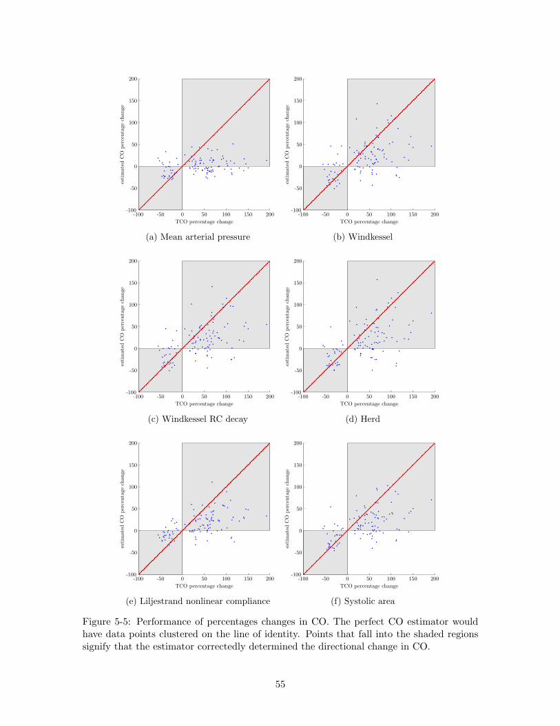
TCO percentage change
esti
mate
dC
Oper
centa
ge
change
-100 -50 0 50 100 150 200-100
-50
0
50
100
150
200
TCO percentage change
esti
mate
dC
Oper
centa
ge
change
-100 -50 0 50 100 150 200-100
-50
0
50
100
150
200
(a) Mean arterial pressure (b) Windkessel
TCO percentage change
esti
mat
edC
Oper
centa
gech
ange
-100 -50 0 50 100 150 200-100
-50
0
50
100
150
200
TCO percentage change
esti
mat
edC
Oper
centa
gech
ange
-100 -50 0 50 100 150 200-100
-50
0
50
100
150
200
(c) Windkessel RC decay (d) Herd
TCO percentage change
esti
mat
edC
Oper
centa
gech
ange
-100 -50 0 50 100 150 200-100
-50
0
50
100
150
200
TCO percentage change
esti
mat
edC
Oper
centa
gech
ange
-100 -50 0 50 100 150 200-100
-50
0
50
100
150
200
(e) Liljestrand nonlinear compliance (f) Systolic area
Figure 5-5: Performance of percentages changes in CO. The perfect CO estimator wouldhave data points clustered on the line of identity. Points that fall into the shaded regionssignify that the estimator correctedly determined the directional change in CO.
55
TCO percentage change
esti
mate
dC
Oper
centa
ge
change
-100 -50 0 50 100 150 200-100
-50
0
50
100
150
200
TCO percentage change
esti
mate
dC
Oper
centa
ge
change
-100 -50 0 50 100 150 200-100
-50
0
50
100
150
200
(a) Systolic area with correction (e) Systolic area with corrected impedance
TCO percentage change
esti
mat
edC
Oper
centa
gech
ange
-100 -50 0 50 100 150 200-100
-50
0
50
100
150
200
TCO percentage change
esti
mat
edC
Oper
centa
gech
ange
-100 -50 0 50 100 150 200-100
-50
0
50
100
150
200
(c) Pressure RMS (d) Godje nonlinear compliance
TCO percentage change
esti
mat
edC
Oper
centa
gech
ange
-100 -50 0 50 100 150 200-100
-50
0
50
100
150
200
TCO percentage change
esti
mat
edC
Oper
centa
gech
ange
-100 -50 0 50 100 150 200-100
-50
0
50
100
150
200
(e) Wesseling Modelflow (f) Constant CO
Figure 5-6: Performance of percentages changes in CO (continued).
56
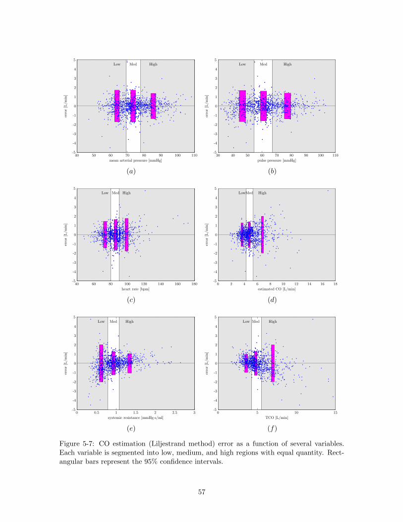
erro
r[L
/min
]
mean arterial pressure [mmHg]
Low Med High
40 50 60 70 80 90 100 110-5
-4
-3
-2
-1
0
1
2
3
4
5
erro
r[L
/min
]
pulse pressure [mmHg]
Low Med High
30 40 50 60 70 80 90 100 110-5
-4
-3
-2
-1
0
1
2
3
4
5
(a) (b)
erro
r[L
/min
]
heart rate [bpm]
Low Med High
40 60 80 100 120 140 160 180-5
-4
-3
-2
-1
0
1
2
3
4
5
erro
r[L
/min
]
estimated CO [L/min]
LowMed High
0 2 4 6 8 10 12 14 16 18-5
-4
-3
-2
-1
0
1
2
3
4
5
(c) (d)
erro
r[L
/min
]
systemic resistance [mmHg·s/ml]
Low Med High
0 0.5 1 1.5 2 2.5 3-5
-4
-3
-2
-1
0
1
2
3
4
5
erro
r[L
/m
in]
TCO [L/min]
Low Med High
0 5 10 15-5
-4
-3
-2
-1
0
1
2
3
4
5
(e) (f)
Figure 5-7: CO estimation (Liljestrand method) error as a function of several variables.Each variable is segmented into low, medium, and high regions with equal quantity. Rect-angular bars represent the 95% confidence intervals.
57
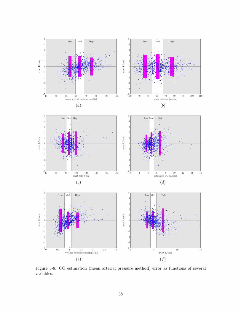
erro
r[L
/min
]
mean arterial pressure [mmHg]
Low Med High
40 50 60 70 80 90 100 110-5
-4
-3
-2
-1
0
1
2
3
4
5
erro
r[L
/min
]
pulse pressure [mmHg]
Low Med High
30 40 50 60 70 80 90 100 110-5
-4
-3
-2
-1
0
1
2
3
4
5
(a) (b)
erro
r[L
/min
]
heart rate [bpm]
Low Med High
40 60 80 100 120 140 160 180-5
-4
-3
-2
-1
0
1
2
3
4
5
erro
r[L
/min
]
estimated CO [L/min]
Low Med High
0 2 4 6 8 10 12 14 16-5
-4
-3
-2
-1
0
1
2
3
4
5
(c) (d)
erro
r[L
/min
]
systemic resistance [mmHg·s/ml]
Low Med High
0 0.5 1 1.5 2 2.5 3-5
-4
-3
-2
-1
0
1
2
3
4
5
erro
r[L
/min
]
TCO [L/min]
Low Med High
0 5 10 15-5
-4
-3
-2
-1
0
1
2
3
4
5
(e) (f)
Figure 5-8: CO estimation (mean arterial pressure method) error as functions of severalvariables.
58
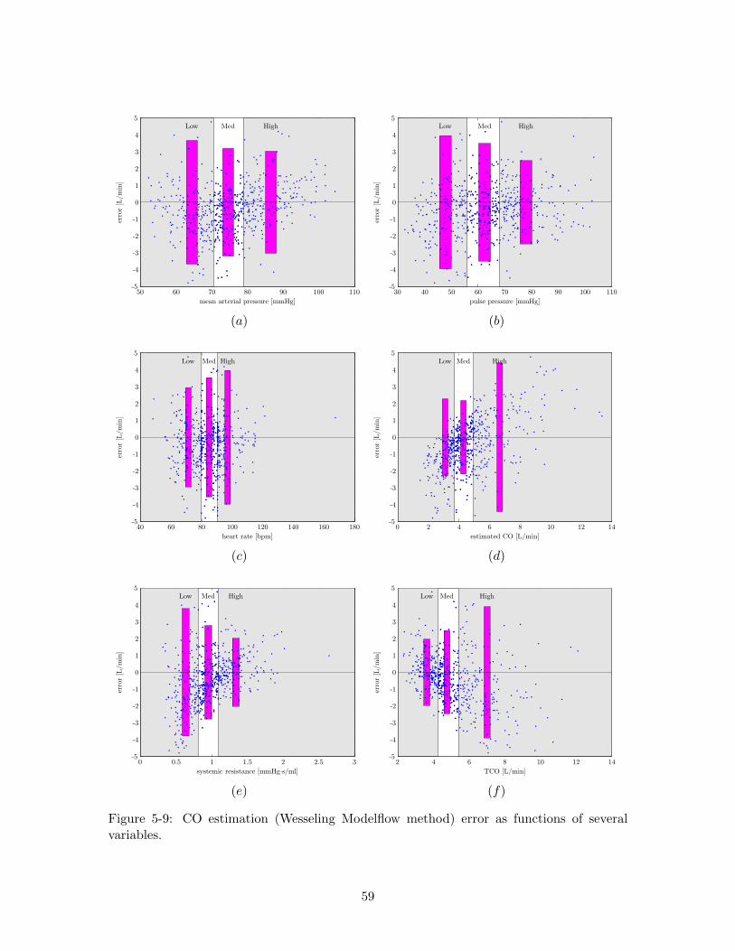
erro
r[L
/min
]
mean arterial pressure [mmHg]
Low Med High
50 60 70 80 90 100 110-5
-4
-3
-2
-1
0
1
2
3
4
5
erro
r[L
/min
]
pulse pressure [mmHg]
Low Med High
30 40 50 60 70 80 90 100 110-5
-4
-3
-2
-1
0
1
2
3
4
5
(a) (b)
erro
r[L
/min
]
heart rate [bpm]
Low Med High
40 60 80 100 120 140 160 180-5
-4
-3
-2
-1
0
1
2
3
4
5
erro
r[L
/min
]
estimated CO [L/min]
Low Med High
0 2 4 6 8 10 12 14-5
-4
-3
-2
-1
0
1
2
3
4
5
(c) (d)
erro
r[L
/min
]
systemic resistance [mmHg·s/ml]
Low Med High
0 0.5 1 1.5 2 2.5 3-5
-4
-3
-2
-1
0
1
2
3
4
5
erro
r[L
/min
]
TCO [L/min]
Low Med High
2 4 6 8 10 12 14-5
-4
-3
-2
-1
0
1
2
3
4
5
(e) (f)
Figure 5-9: CO estimation (Wesseling Modelflow method) error as functions of severalvariables.
59
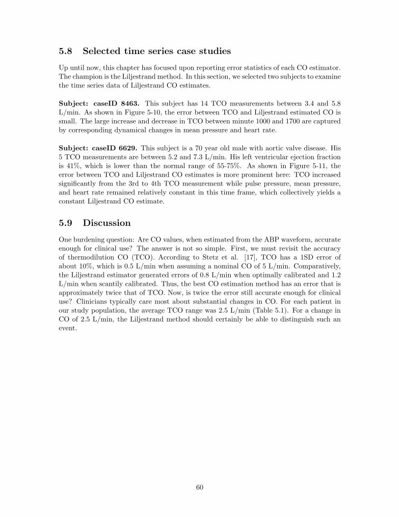
5.8 Selected time series case studies
Up until now, this chapter has focused upon reporting error statistics of each CO estimator.The champion is the Liljestrand method. In this section, we selected two subjects to examinethe time series data of Liljestrand CO estimates.
Subject: caseID 8463. This subject has 14 TCO measurements between 3.4 and 5.8L/min. As shown in Figure 5-10, the error between TCO and Liljestrand estimated CO issmall. The large increase and decrease in TCO between minute 1000 and 1700 are capturedby corresponding dynamical changes in mean pressure and heart rate.
Subject: caseID 6629. This subject is a 70 year old male with aortic valve disease. His5 TCO measurements are between 5.2 and 7.3 L/min. His left ventricular ejection fractionis 41%, which is lower than the normal range of 55-75%. As shown in Figure 5-11, theerror between TCO and Liljestrand CO estimates is more prominent here: TCO increasedsignificantly from the 3rd to 4th TCO measurement while pulse pressure, mean pressure,and heart rate remained relatively constant in this time frame, which collectively yields aconstant Liljestrand CO estimate.
5.9 Discussion
One burdening question: Are CO values, when estimated from the ABP waveform, accurateenough for clinical use? The answer is not so simple. First, we must revisit the accuracyof thermodilution CO (TCO). According to Stetz et al. [17], TCO has a 1SD error ofabout 10%, which is 0.5 L/min when assuming a nominal CO of 5 L/min. Comparatively,the Liljestrand estimator generated errors of 0.8 L/min when optimally calibrated and 1.2L/min when scantily calibrated. Thus, the best CO estimation method has an error that isapproximately twice that of TCO. Now, is twice the error still accurate enough for clinicaluse? Clinicians typically care most about substantial changes in CO. For each patient inour study population, the average TCO range was 2.5 L/min (Table 5.1). For a change inCO of 2.5 L/min, the Liljestrand method should certainly be able to distinguish such anevent.
60
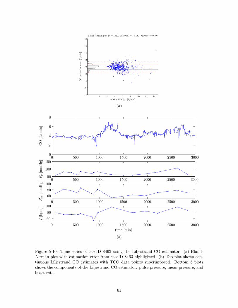
(CO + TCO)/2 [L/min]
CO
esti
mati
on
erro
r[L
/m
in]
Bland-Altman plot (n = 1062, µ(error) = −0.06, σ(error) = 0.79)
0 2 4 6 8 10 12 14-8
-6
-4
-2
0
2
4
6
8
(a)
CO
[L/m
in]
Pp
[mm
Hg]
Pm
[mm
Hg]
f[b
pm
]
time [min]
0 500 1000 1500 2000 2500 3000
0 500 1000 1500 2000 2500 3000
0 500 1000 1500 2000 2500 3000
0 500 1000 1500 2000 2500 3000
60
80
100
60
80
100
50
100
150
0
2
4
6
8
(b)
Figure 5-10: Time series of caseID 8463 using the Liljestrand CO estimator. (a) Bland-Altman plot with estimation error from caseID 8463 highlighted. (b) Top plot shows con-tinuous Liljestrand CO estimates with TCO data points superimposed. Bottom 3 plotsshows the components of the Liljestrand CO estimator: pulse pressure, mean pressure, andheart rate.
61
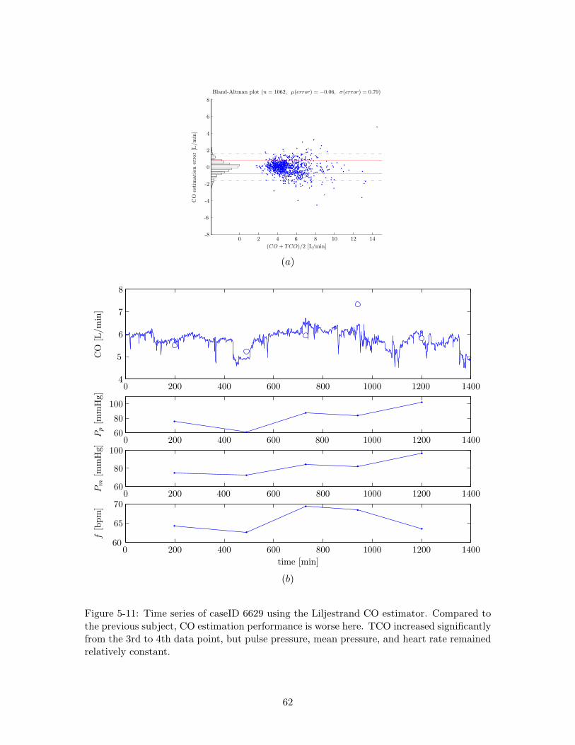
(CO + TCO)/2 [L/min]
CO
esti
mati
on
erro
r[L
/m
in]
Bland-Altman plot (n = 1062, µ(error) = −0.06, σ(error) = 0.79)
0 2 4 6 8 10 12 14-8
-6
-4
-2
0
2
4
6
8
(a)
CO
[L/m
in]
Pp
[mm
Hg]
Pm
[mm
Hg]
f[b
pm
]
time [min]
0 200 400 600 800 1000 1200 1400
0 200 400 600 800 1000 1200 1400
0 200 400 600 800 1000 1200 1400
0 200 400 600 800 1000 1200 1400
60
65
70
60
80
100
60
80
100
4
5
6
7
8
(b)
Figure 5-11: Time series of caseID 6629 using the Liljestrand CO estimator. Compared tothe previous subject, CO estimation performance is worse here. TCO increased significantlyfrom the 3rd to 4th data point, but pulse pressure, mean pressure, and heart rate remainedrelatively constant.
62
Chapter 6
Conclusions and Future Research
6.1 Summary
In this thesis we have presented and evaluated 11 of the established cardiac output estima-tion methods using ABP waveform data from the MIMIC II database.
Chapter 2 discussed the theoretical basis of each CO estimation method. The simplestmethod was based upon a drastically simplified model of the cardiovascular system. Themost complex method, Wesseling’s modelflow, was based upon a model with many nonlin-earities in an attempt to more accurately characterize the dynamics of the cardiovascularsystem. Chapter 2 concluded with a discussion on the fundamental limitations of estimatingCO using ABP waveforms.
Chapter 3 addressed one limitation that hindered CO estimation performance: ABPwaveform quality. The signal abnormality index (SAI) algorithm presented in this chapterattempted to flag regions of ABP waveform of poor quality. In defining what constitutes apoor ABP waveform, we tried to be as objective as as possible. Output of the algorithmwas mostly in concordance with a human expert and proven to be effective in reducing COestimation error.
Chapter 4 presented our methods for evaluating the CO estimators. We designed algo-rithms to extract pressure and temporal features from the ABP waveform. We integratedthe SAI algorithm to ensure that extremely poor ABP waveforms are eliminated. We de-signed calibration techniques, which is necessary for CO estimators to produce absolutevalues in liters per minute. In absence of calibration, we presented a technique to comparepercentage changes in gold-standard CO with percentage changes in estimated CO.
Chapter 5 showed the performance of the 11 CO estimators. For absolute CO estima-tion, the Liljestrand CO estimator was clearly the champion. It generated errors of 0.8L/min when optimally calibrated and 1.2 L/min when scantily calibrated. Whether suchspecifications are meritable for clinical use is ultimately up to the decision of a clinician.However, it should be noted that patients with life-threatening problems often have COfluctuations significantly beyond 1.2 L/min. For each patient in our study population, theaverage thermodilution CO range was 2.5 L/min. Thus, the Liljestrand estimator shouldbe able to detect such large changes in CO.
63

6.2 Suggestions for future research
As this thesis draws to a close, inevitably there are research tasks not accomplished butwould be plausible extensions of this thesis. There are also interesting research tangents toembark on.
Algorithmic improvements. As evidenced by the 11 CO estimators studied in thisthesis, previous research on improving CO estimation have been mostly in the creation ofnew methods from first principles or in the modification of existing methods. An alternativeapproach to improve CO estimation is to optimally combine the existing methods. It is likelythat one CO algorithm works better than another under different physiologic situations.The detailed error analysis of the Liljestrand algorithm (Figure 5-7) clearly shows thatthis algorithm is more accurate when mean arterial pressure is over 80mmHg, heart rateis less than 80bpm, estimated CO is less than 5L/min, and systemic resistance is greaterthan 1 mmHg·s/ml. We can perform similar error analysis on the remaining 10 algorithms,perhaps as a function of even more physiologic information obtained from lab tests andnursing notes. Then, a master algorithm may be developed to optimally choose the COestimator(s) that will likely be most accurate for each particular patient.
The Signal Abnormality Index (SAI) algorithm works reasonably well but certainlyhas potential for improvement. The current SAI logic is composed of a series of staticcriteria imposed on pressure values and beat-to-beat durations (Table 3.2). Each criterionis independent of each other. One possible improvement would be to dynamically changethe thresholds for each criterion. For example, beat-to-beat variations of systolic bloodpressure is likely larger in patients with large pulse pressure than ones with small pulsepressure. Thus, abnormality criteria 7 in Table 3.2 should be a function of pulse pressurerather than the constant value of 20mmHg. However, with rising complexity, the degrees offreedom in the algorithm rises, and one must attempt to avoid over-training the algorithmto a particular data set.
Live clinical evaluations. All research in this thesis have been in analyzing data retro-spectively. It does not prove that continuous cardiac output monitoring with such a level ofaccuracy can indeed aid in clinical decision making. It would be an interesting investigationto build a CO bedside monitoring system (perhaps in addition to providing CO estimates,the system would generate alarms when CO exceeds a nominal range or undergoes dra-matic change) and use it in a hospital to see whether such a system provides clinicians withvaluable information that is not available otherwise.
Stroke volume variability. Variabilities of CO estimates are different amongst the esti-mation methods. By removing heart rate out of the equation, we can obtain variability ofstroke volume, which raises a couple of interesting questions. First, which method of ob-taining stroke volume gives the variability level that closest resembles reality? Second, doesan increase in stroke volume variability of a patient forewarn the onset of certain diseaseprocesses? Is stroke volume variability closely coupled with heart rate variability? Queryingfor “heart rate variability” yields 5644 articles on PubMed online. Querying “stroke volumevariability” yields a scant 6 articles, which means there may be new research potential here.
64

Appendix A
Notation Summary
Table A.1: Commonly used acronyms and symbolssymbol description units
Q, CO cardiac output L/minq(t) instantaneous pulsatile flow ml/sP (t), ABP arterial blood pressure mmHgPm mean arterial pressure mmHgPs systolic pressure mmHgPd diastolic pressure mmHgPp pulse pressure (Ps − Pd) mmHgf heart rate beats per minuteT beat duration (60/f) secTs duration of systole secTd duration of diastole (T − Ts) secR, SV R, PV R systemic resistance mmHg·s/mlC arterial capacitance (compliance) ml/mmHgAs area under P (t) during systole mmHg·s
65

66
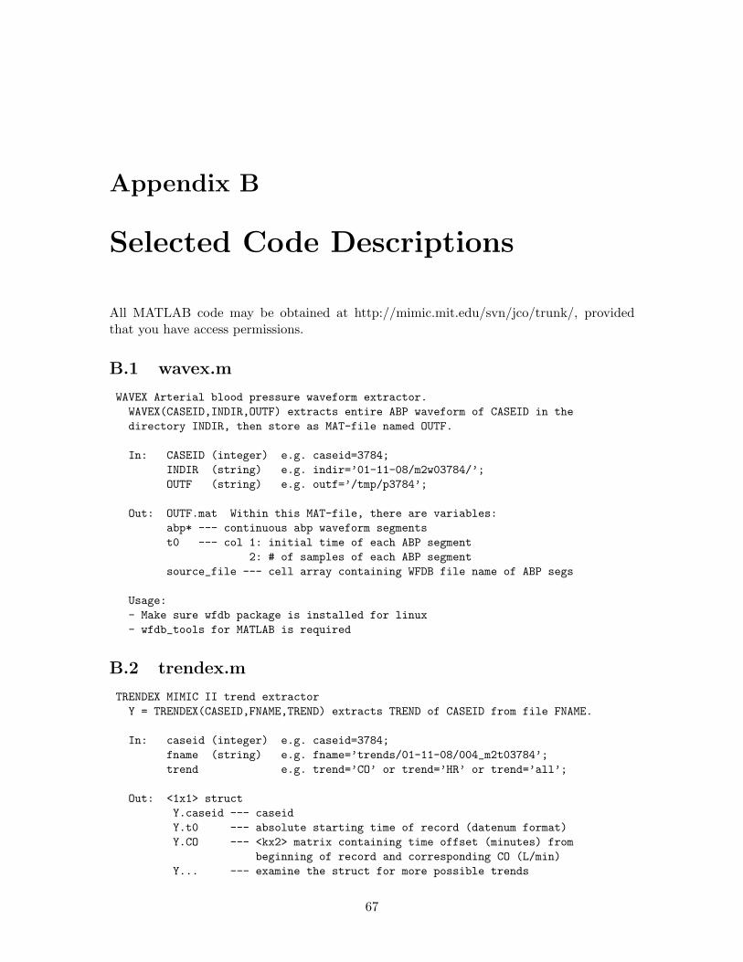
Appendix B
Selected Code Descriptions
All MATLAB code may be obtained at http://mimic.mit.edu/svn/jco/trunk/, providedthat you have access permissions.
B.1 wavex.m
WAVEX Arterial blood pressure waveform extractor.
WAVEX(CASEID,INDIR,OUTF) extracts entire ABP waveform of CASEID in the
directory INDIR, then store as MAT-file named OUTF.
In: CASEID (integer) e.g. caseid=3784;
INDIR (string) e.g. indir=’01-11-08/m2w03784/’;
OUTF (string) e.g. outf=’/tmp/p3784’;
Out: OUTF.mat Within this MAT-file, there are variables:
abp* --- continuous abp waveform segments
t0 --- col 1: initial time of each ABP segment
2: # of samples of each ABP segment
source_file --- cell array containing WFDB file name of ABP segs
Usage:
- Make sure wfdb package is installed for linux
- wfdb_tools for MATLAB is required
B.2 trendex.m
TRENDEX MIMIC II trend extractor
Y = TRENDEX(CASEID,FNAME,TREND) extracts TREND of CASEID from file FNAME.
In: caseid (integer) e.g. caseid=3784;
fname (string) e.g. fname=’trends/01-11-08/004_m2t03784’;
trend e.g. trend=’CO’ or trend=’HR’ or trend=’all’;
Out: <1x1> struct
Y.caseid --- caseid
Y.t0 --- absolute starting time of record (datenum format)
Y.CO --- <kx2> matrix containing time offset (minutes) from
beginning of record and corresponding CO (L/min)
Y... --- examine the struct for more possible trends
67

Usage:
- Make sure wfdb package is installed for linux
- wfdb_tools for MATLAB is required
- if 3rd argument is ’all’, then all trends of CASEID are obtained
B.3 wabp.m
WABP ABP waveform onset detector.
r = WABP(ABP) obtains the onset time (in samples)
of each beat in the ABP waveform.
In: ABP (125Hz sampled)
Out: Onset sample time
Usage:
- ABP waveform must have units of mmHg
B.4 abpfeature.m
ABPFEATURE ABP waveform feature extractor.
r = ABPFEATURE(ABP,ONSETTIMES) extracts features from ABP waveform such
as systolic pressure, mean pressure, etc.
In: ABP (125Hz sampled), times of onset (in samples)
Out: Beat-to-beat ABP features
Col 1: Time of systole [samples]
2: Systolic BP [mmHg]
3: Time of diastole [samples]
4: Diastolic BP [mmHg]
5: Pulse pressure [mmHg]
6: Mean pressure [mmHg]
7: Beat Period [samples]
8: mean_dyneg
9: End of systole time 0.3*sqrt(RR) method
10: Area under systole 0.3*sqrt(RR) method
11: End of systole time 1st min-slope method
12: Area under systole 1st min-slope method
Usage:
- OnsetTimes must be obtained using wabp.m
B.5 jSQI.m
JSQI ABP waveform signal quality index.
[BEATQ, R] = JSQI(FEATURES, ONSET, ABP) returns a binary signal quality
assessment of each beat in ABP. This algorithm relies on detecting
abnormalities of numeric values in FEATURES and ONSET.
In: FEATURES <mx12> --- features extracted from ABP using abpfeature.m
ONSET <nx1> --- onset times of ABP using wabp.m
ABP <px1> --- arterial blood pressure waveform (125Hz sampled)
68
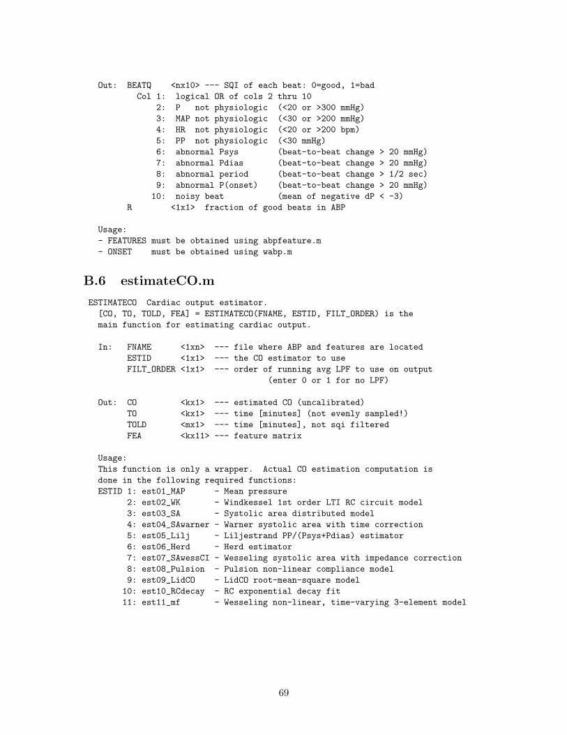
Out: BEATQ <nx10> --- SQI of each beat: 0=good, 1=bad
Col 1: logical OR of cols 2 thru 10
2: P not physiologic (<20 or >300 mmHg)
3: MAP not physiologic (<30 or >200 mmHg)
4: HR not physiologic (<20 or >200 bpm)
5: PP not physiologic (<30 mmHg)
6: abnormal Psys (beat-to-beat change > 20 mmHg)
7: abnormal Pdias (beat-to-beat change > 20 mmHg)
8: abnormal period (beat-to-beat change > 1/2 sec)
9: abnormal P(onset) (beat-to-beat change > 20 mmHg)
10: noisy beat (mean of negative dP < -3)
R <1x1> fraction of good beats in ABP
Usage:
- FEATURES must be obtained using abpfeature.m
- ONSET must be obtained using wabp.m
B.6 estimateCO.m
ESTIMATECO Cardiac output estimator.
[CO, TO, TOLD, FEA] = ESTIMATECO(FNAME, ESTID, FILT_ORDER) is the
main function for estimating cardiac output.
In: FNAME <1xn> --- file where ABP and features are located
ESTID <1x1> --- the CO estimator to use
FILT_ORDER <1x1> --- order of running avg LPF to use on output
(enter 0 or 1 for no LPF)
Out: CO <kx1> --- estimated CO (uncalibrated)
TO <kx1> --- time [minutes] (not evenly sampled!)
TOLD <mx1> --- time [minutes], not sqi filtered
FEA <kx11> --- feature matrix
Usage:
This function is only a wrapper. Actual CO estimation computation is
done in the following required functions:
ESTID 1: est01_MAP - Mean pressure
2: est02_WK - Windkessel 1st order LTI RC circuit model
3: est03_SA - Systolic area distributed model
4: est04_SAwarner - Warner systolic area with time correction
5: est05_Lilj - Liljestrand PP/(Psys+Pdias) estimator
6: est06_Herd - Herd estimator
7: est07_SAwessCI - Wesseling systolic area with impedance correction
8: est08_Pulsion - Pulsion non-linear compliance model
9: est09_LidCO - LidCO root-mean-square model
10: est10_RCdecay - RC exponential decay fit
11: est11_mf - Wesseling non-linear, time-varying 3-element model
69

70
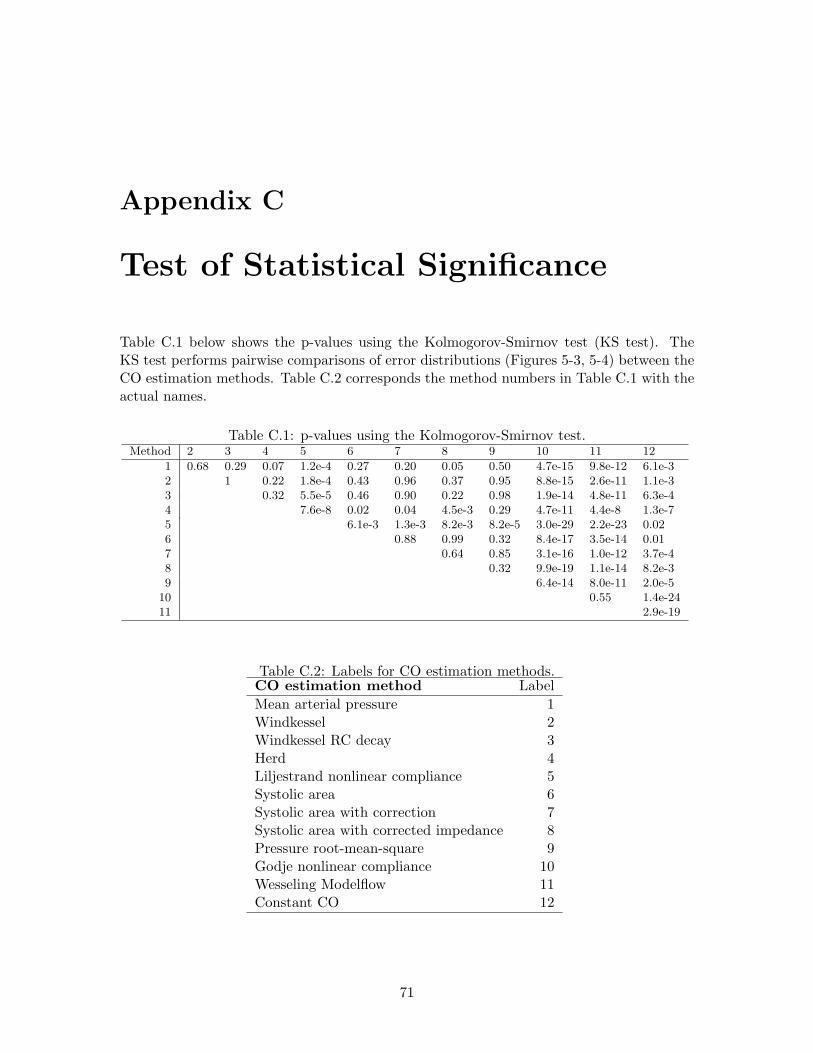
Appendix C
Test of Statistical Significance
Table C.1 below shows the p-values using the Kolmogorov-Smirnov test (KS test). TheKS test performs pairwise comparisons of error distributions (Figures 5-3, 5-4) between theCO estimation methods. Table C.2 corresponds the method numbers in Table C.1 with theactual names.
Table C.1: p-values using the Kolmogorov-Smirnov test.Method 2 3 4 5 6 7 8 9 10 11 12
1 0.68 0.29 0.07 1.2e-4 0.27 0.20 0.05 0.50 4.7e-15 9.8e-12 6.1e-3
2 1 0.22 1.8e-4 0.43 0.96 0.37 0.95 8.8e-15 2.6e-11 1.1e-3
3 0.32 5.5e-5 0.46 0.90 0.22 0.98 1.9e-14 4.8e-11 6.3e-4
4 7.6e-8 0.02 0.04 4.5e-3 0.29 4.7e-11 4.4e-8 1.3e-7
5 6.1e-3 1.3e-3 8.2e-3 8.2e-5 3.0e-29 2.2e-23 0.02
6 0.88 0.99 0.32 8.4e-17 3.5e-14 0.01
7 0.64 0.85 3.1e-16 1.0e-12 3.7e-4
8 0.32 9.9e-19 1.1e-14 8.2e-3
9 6.4e-14 8.0e-11 2.0e-5
10 0.55 1.4e-24
11 2.9e-19
Table C.2: Labels for CO estimation methods.CO estimation method Label
Mean arterial pressure 1Windkessel 2Windkessel RC decay 3Herd 4Liljestrand nonlinear compliance 5Systolic area 6Systolic area with correction 7Systolic area with corrected impedance 8Pressure root-mean-square 9Godje nonlinear compliance 10Wesseling Modelflow 11Constant CO 12
71

72

Bibliography
[1] HC Bazett. An analysis of the time-relations of electrocardiograms. Heart, 7:353–370,1920.
[2] RM Berne, MN Levy, BM Koeppen, and BA Stanton. Physiology. Mosby, 5th edition,2004.
[3] JM Bland and DG Altman. Statistical methods for assessing agreement between twomethods of clinical measurement. The Lancet, pages 307–310, 1986.
[4] J Bourgeois, B Gilbert, D Donald, and E Wood. Characteristics of aortic diastolicpressure decay with application to continuous monitoring of changes in peripheralvascular resistance. Circulation Research, 35:56–66, 1974.
[5] J Erlanger and BR Hooker. An experimental study of blood pressure and pulse-pressurein man. Johns Hopkins Hospital Report, 12:145–378, 1904.
[6] O Godje, P Lamm, C Schmitz, M Theil, and B Reichart. Continuous, less invasive,hemodynamic monitoring in intensive care after cardiac surgery. Thoracic Cardiovas-
cular Surgery, 46:242–249, 1998.
[7] JA Herd, NR Leclair, and W Simon. Arterial pressure pulse contours during hemor-rhage in anesthetized dogs. Journal of Applied Physiology, 21(6):1864–1868, 1966.
[8] LL Huntsman, DK Stewart, SR Barnes, SB Franklin, JS Colocousis, and EA Hes-sel. Noninvasive doppler determination of cardiac output in man: clinical validation.Circulation, 67:593–602, 1983.
[9] M Jonas, D Hett, and J Morgan. Real time, continuous monitoring of cardiac outputand oxygen delivery. International Journal of Intensive Care, 9(2), 2002.
[10] NT Kouchoukos, LC Sheppard, and DA McDonald. Estimation of stroke volume inthe dog by a pulse contour method. Circulation Research, 26:611–623, 1970.
[11] GJ Langewouters, KH Wesseling, and WJA Goedhard. The static elastic propertiesof 45 human thoracic and 20 abdominal aortas in vitro and the parameters of a newmodel. Journal of Biomechanics, 17:425–435, 1984.
[12] G Liljestrand and E Zander. Vergleichende bestimmungen des minutenvolumens desherzens beim menschen mittels der stickoxydulmethode und durch blutdruckmessung.Z Ges Exp Med, 59:105–122, 1928.
[13] RG Mark. MIT course notes for 6.022J quantitative physiology — cardiovascularmechanics. http://mit.edu/6.022j/www/, 2005.
73
[14] R Mukkamala, AT Reisner, RG Mark, and RJ Cohen. Continuous cardiac outputmonitoring by peripheral blood pressure waveform analysis. IEEE Transactions on
Biomedical Engineering, 53:459–467, 2006.
[15] WW Nichols and MF O’Rourke. McDonald’s Blood Flow in Arteries. Arnold, 4thedition, 1998.
[16] M Saeed, C Lieu, G Raber, and RG Mark. MIMIC II: A massive temporal ICUpatient database to support research in intelligent patient monitoring. In Computers
in Cardiology, volume 29, pages 641–644, 2002.
[17] CW Stetz, RG Miller, GE Kelly, and TA Raffin. Reliability of the thermodilutionmethod in the determination of cardiac output in clinical practice. American Review
of Respiratory Disease, 126(6):1001–4, 1982.
[18] JJ van Lieshout and KH Wesseling. Editorial II: Continuous cardiac output by pulsecontour analysis? British Journal of Anaesthesia, 86(4):467–468, 2001.
[19] HR Warner, HJC Swan, DC Connolly, RG Tompkins, and EH Wood. Quantitation ofbeat-to-beat changes in stroke volume from the aortic pulse contour in man. Journal
of Applied Physiology, 5:495–507, 1953.
[20] KH Wesseling, R Jansen, J Settels, and J Schreuder. Computation of aortic flowfrom pressure in humans using a nonlinear, three-element model. Journal of Applied
Physiology, 74(5):2566–2573, 1993.
[21] KH Wesseling, BD Wit, JAP Weber, and NT Smith. A simple device for the continuousmeasurement of cardiac output. Advanced Cardiovascular Physiology, 5(2):16–52, 1983.
[22] W Zong, T Heldt, GB Moody, and RG Mark. An open-source algorithm to detectonset of arterial blood pressure pulses. In Computers in Cardiology, volume 30, pages259–262, 2003.
74