cardinal direction relations in qualitative spatial reasoning

International Journal of Computer Science & Information Technology (IJCSIT) Vol 6, No 1, February 2014

DOI : 10.5121/ijcsit.2014.6101 1

Cardinal Direction Relations in Qualitative

Spatial Reasoning

Chaman L. Sabharwal and Jennifer L. Leopold

Missouri University of Science and Technology Rolla, Missouri, USA – 65409

ABSTRACT

Representation and reasoning with spatial information is a fundamental aspect of artificial

intelligence. Qualitative methods have become prominent in spatial reasoning. In geophysical explorations,

one of the aspects is to determine compass direction between the regions. In this paper, we present an

efficient approach to cardinal directions between free form regions. The development is very simple,

mathematically sound and can be implemented efficiently. The extension to 3D is seamless; it needs no

additional formulation for transition from 2D to 3D.It has no adverse impact on the computational

efficiency, as the technique is akin to 2D. This work is directly applicable to geographical information

systems for location determination, robot navigation, and spatio-temporal networks databases where

direction changes frequently.

KEYWORDS

Cardinal Directions, Spatial Reasoning,Composition,Partialand Whole Regions

1. INTRODUCTION

Representation and reasoning with spatial information is a fundamental aspect of artificial intelligence. There are two forms ofspatial knowledge, exact and inexact knowledge, usually referred to as quantitative and qualitative knowledge.The qualitative methods have become prominent in spatial reasoning. There are various ways to describe spatial knowledge, that is, temporal size, shape, directional orientation or topological connectivity relations.

There are three types of spatial relations: Allen’s 13-relation calculus for spatio-temporal relations [1], Freksa’scardinal directional relations [2], and the Randell-Cui-Cohn RCC8 relations [3,4]. In this paper we will concentrate on cardinal direction relations and improve upon the existing methods for representation and reasoning.

Orientation refers to relative position of regions with respect to each other. The directional relation between a targetobject and a reference object is calculated with respect to a frame of reference such as a base coordinate system where position and orientation is specified.The design for efficient representation and calculation of cardinal relations between regionsispervasive in spatial reasoning.

For example, a car parked in front of the garage may mean several things; it depends on the location of the garage opening.If the garage has an opening on the side of the house, it could


2

mean the car is in the driveway literally in front of the garage, that is, the car is on side of the house.Also it could mean that the car is on the street but closest to the garage.

The paper is organized as follows: Section 2 describes the background on space portioning, grid creation, representation, and interpretation. Section 3 gives the mathematical foundations for grid calculation, grid representation semantics, and atomic and complex directional relation computation technique. Section 4 discussesthe extension to 3D.Section 5presents future direction. Section 6 describes our conclusions followed by references in Section 7.

2. BACKGROUND

2.1.Space Partition

In 2D, cardinal or compass directions are denoted by NW, N, NE, W, E, SW, S, SE, and O relative to the center O, see Fig.1.

Fig. 1. Compass directions: N, S, E, W, NW, NE, SW, SE

A 2D region divides the space into nine parts, one region bounded and eight unbounded sections: the center section O is a bounded rectangle, whereas sections NW, N, NE, W, E, SW, S, SE have unbounded extent, see Fig. 2. The symbols play a dual role: (1) they represent the orientation direction of the location relative to O, and (2) they represent the location area. Thus these directional symbols may be used to represent location anddirection. In order to avoid any ambiguity, we refer to all parts in Fig. 2as regions or sections or locations interchangeablyin this discussion.

Fig. 2. Partition of 2D space into 9 sections.The center section is a bounded region; the other eight sections are unbounded.

We will also use Fig. 2 in the context of twoarbitrary objects. Ifan object A is in the upper left

corner,NW, and an object B is in the center cell, O, we denote the direction of A relative to B by dir(B,A) which is symbolicallyNW.


3

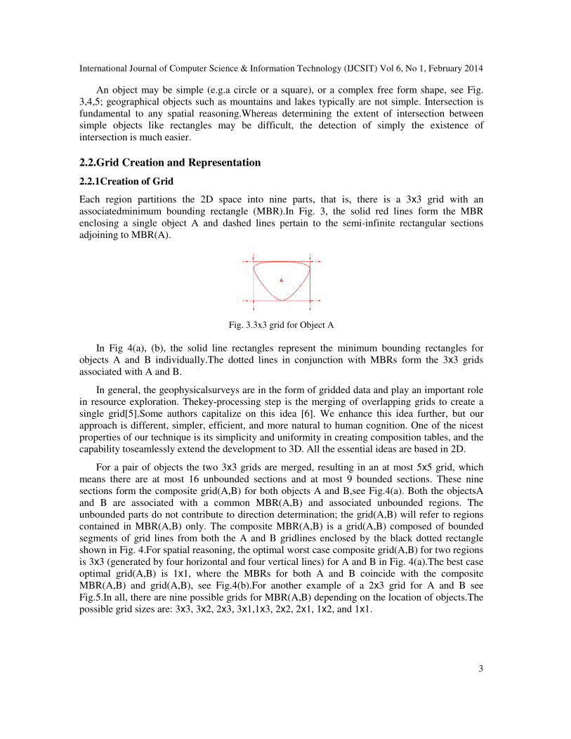
An object may be simple (e.g.a circle or a square), or a complex free form shape, see Fig. 3,4,5; geographical objects such as mountains and lakes typically are not simple. Intersection is fundamental to any spatial reasoning.Whereas determining the extent of intersection between simple objects like rectangles may be difficult, the detection of simply the existence of intersection is much easier.

2.2.Grid Creation and Representation

2.2.1Creation of Grid

Each region partitions the 2D space into nine parts, that is, there is a 3x3 grid with an associatedminimum bounding rectangle (MBR).In Fig. 3, the solid red lines form the MBR enclosing a single object A and dashed lines pertain to the semi-infinite rectangular sections adjoining to MBR(A).

Fig. 3.3x3 grid for Object A

In Fig 4(a), (b), the solid line rectangles represent the minimum bounding rectangles for objects A and B individually.The dotted lines in conjunction with MBRs form the 3x3 grids associated with A and B.

In general, the geophysicalsurveys are in the form of gridded data and play an important role in resource exploration. Thekey-processing step is the merging of overlapping grids to create a single grid[5].Some authors capitalize on this idea [6]. We enhance this idea further, but our approach is different, simpler, efficient, and more natural to human cognition. One of the nicest properties of our technique is its simplicity and uniformity in creating composition tables, and the capability toseamlessly extend the development to 3D. All the essential ideas are based in 2D.

For a pair of objects the two 3x3 grids are merged, resulting in an at most 5x5 grid, which means there are at most 16 unbounded sections and at most 9 bounded sections. These nine sections form the composite grid(A,B) for both objects A and B,see Fig.4(a). Both the objectsA and B are associated with a common MBR(A,B) and associated unbounded regions. The unbounded parts do not contribute to direction determination; the grid(A,B) will refer to regions contained in MBR(A,B) only. The composite MBR(A,B) is a grid(A,B) composed of bounded segments of grid lines from both the A and B gridlines enclosed by the black dotted rectangle shown in Fig. 4.For spatial reasoning, the optimal worst case composite grid(A,B) for two regions is 3x3 (generated by four horizontal and four vertical lines) for A and B in Fig. 4(a).The best case optimal grid(A,B) is 1x1, where the MBRs for both A and B coincide with the composite MBR(A,B) and grid(A,B), see Fig.4(b).For another example of a 2x3 grid for A and B see Fig.5.In all, there are nine possible grids for MBR(A,B) depending on the location of objects.The possible grid sizes are: 3x3, 3x2, 2x3, 3x1,1x3, 2x2, 2x1, 1x2, and 1x1.


4

2.2.2 GridInterpretation

In order to determine the directional relation between two regions, considerablecomputational effort can bespent in the processing of Object Intersection Matrices (OIM) [6,7]. The authors of previous work maycreate various classes of matrices and definespecialized functions for those matrices: an object intersection grid matrix, an object intersection grid space matrix, an intersection location function, an intersection location table, an object intersection matrix, and an intersection interpretation function.Also required is a handcrafted9x9 table to determine the direction between any two locations in the grid.No insight into composition of relations is given. The grid representation and interpretation is not without ambiguities.For example, in Fig. 5, A is completely on one side of B.Theinterpretation for this given in [6] is: A is partly to the north of B, partly to northeast of B, and partly northwest of B.An accurate interpretation would bethat the whole of A is to the north of a part of B, northwest of a part of B, and northeast of a part of B, whereas B is partly to the southwest, partly to the south, and partly to the southeast of the whole of A. Thus the converse relation interpretation does not hold good in the original statement.

(a) (b)

Fig. 4. (a) 3x3 gird enclosing A and B (b) 1x1 grid enclosing A and B

Fig. 5. Example of 2x3 grid enclosing objects A and B

We presenta rigorous method for representing configurations for a pair of objects A and B, which is not envisioned otherwise.This way we showthat our approach is complete and analytically sound. In Section 3, weprovide a very simple,mathematically sound, provably correct formulation to determine cardinal directions between objects. We also show that our formulation extends naturally to 3D with no additional conceptual development of formulation.Even the slightest gain in computational efficiency has a significant impact.

3. MATHEMATICAL DEVELOPMENT

3.1. Grid Calculation

We use the notation, xAm for maximum lower bound of the x-coordinates of all points in A;

xAMrepresents the least upper bound of all the x coordinates in A; similarly yA

mand yAMrepresent

thebounds for the y-coordinates of all points in A.All the points in the region A lie in the


5

rectangle {(x,y): xAm ≤ x ≤ xA

M, yAm ≤ y ≤yA

M}.The othereight unbounded parts are to the N,S,E,W,NW,SW,NE,SE as seen in Fig. 2.For the object A, the minimum bounding rectangle, MBR(A), becomes O(A) or simply O, the center of grid(A)

O(A)= {(x,y): xAm ≤ x ≤ xA

M, yAm ≤ y ≤ yA

M }

The other sections become

N(A) = {(x,y): xAm ≤ x ≤ xA

M, y >yAM }

S(A) = {(x,y): xAm ≤ x ≤ xA

M, y <yAm }

E(A) = {(x,y): xAM< x, yA

m ≤ y ≤ yAM }

W(A) = {(x,y): x <xAm , yA

m ≤ y ≤yAM }

NE(A) = {(x,y): x >xAM, y >yA

M } NW(A) = {(x,y): x <xA

m , y >yAM }

SE(A) = {(x,y): xAM< x, y <yA

m } SW(A) = {(x,y): x <xA

m, y <yAm }

These definitions are slightly different from those in[6];in that work they are defined in an ad hoc mannerdevoid of symmetry where a part of the boundary belongs to O(A), a part of it does not, and similarly for other cells.

NowMBR(A)= {(x,y): xAm ≤ x ≤ xA

M, yAm ≤ y ≤ yA

M} and represents four grid lines x=xAm,

x=xAM; y=yA

m, y=yAM as well, and gridlines for MBR(B)are: x=xB

m, x=xBM;y=yB

m, y=yBM.These

grid lines are used to createa grid for the composite minimum bounding rectangle for both A and B denoted byMBR(A,B) ={(x,y): min(xA

m, xBm )≤ x ≤ max(xA

M, xBM),min(yA

m, yBm )≤ y ≤

max(yAM, yB

M)}.

The number of grid line segments in MBR(A,B) depends on how many grid lines in A coincide with grid lines in B.If all grid lines are distinct, there are 4 vertical and 4 horizontal grid lines.The grid(A,B) is at most 5x5. MBR(A,B) is associated withan at most 3x3 bounded grid(A,B). From now on, we will refer to grid(A,B) as only that part which is within MBR(A,B); the grid(A,B) is at most 3x3.Let us start with 3x3 grid(A,B), then later we will generalize our findings to any possible pxqgrid(A,B), see Section 3.1.In general, the composite grid(A,B) for objects A and B is pxqfor 1≤p, q≤3 wherep and q are defined by

p= 3 - |{yAm, yA

M}∩{ yBm, yB

M}|

q =3 - |{xAm, xA

M}∩{ xBm, xB

M}|

3.2.Grid Representation Semantics

The grid(A,B) is at most 3x3. For a 3x3 grid, the cells are conventionally labeled asO, N, S, E, W, NW, NE, SW, SE,consistent with Fig. 2 and Table 1.

Table 1. Table Of DirectionsRelative to the Center O

NW N NE

W SS=O E

SW S SE

The grid(A,B) with direction values NW, N, NE, W, O, E, SW, S, SE, may be indexed in

anyway. Some authors [6] used the standard matrix-indexing scheme shown in Table 2.


6

Table 2. Standard Grid(A,B) Indexing Scheme

(1,1) (1,2) (1,3)

(2,1) (2,2) (2,3)

(3,1) (3,3) (3,3)

We present a different indexing scheme based on negative indexes[8]; see Table 3 where cell NW is indexed with ordered pair (-1,1). Thus (-1,1) also represents the direction of NW with respect to O.Similarly other indexes are directions of grid cells with respect to O.If an object intersects a cell, thedirection of the cell with respect to O is simply the index of the cell.These indexes play a dual role: the direction of the cell as well as the location of the cell. No extra work is needed for processing such index labels.Thus Table 3 is self-sufficient for deriving position and direction.This simple indexing scheme lends itself naturally to computations of relations efficiently.

Later we will generalize this indexing technique in two ways: (1)how to index pxq grids when p≠3 or q≠3, and (2) how to label cells in 3D in Section 4.Since the NW section is unbounded, any point in NW can be represented by(-u,v) for positive u and v. To accommodate all such representations consistent with indexing, our technique really identifies the whole NW region

with (-1,1) by NW≡(sign(x),sign(y)) where (x,y) is any point in the NW section. Thus Table 3 maps the symbolic orientation of every cell relative to the origin to an ordered pair.This indexing scheme is very useful in computing the directional relations.

Table 3. New Indexing of the Cells in Grid(A,B)

(-1,1) (0,1) (1,1)

(-1,0) (0,0) (1,0)

(-1,-1) (0,-1) (1,-1)

3.3. Cardinal DirectionRelations

3.3.1. Atomic Relations

The cell location, object intersection, and orientation can be treated uniformly here. For example, in Table3symbol (-1,1) refers to the northwest section of the grid;alsothis is to the northwest direction relative to the center cell. Thedirection of A relative to O isdenoted by dir(O,A)and is represented by {(-1,1)}.Soon we will see that set notation is more consistent with the complex direction relations. The other atomic directions are defined similarly consistent with Table 3 when an object A intersects a corresponding cell.It is simple for an object intersecting only one cell. The only thing needed is the location where the object intersects in grid(A,B).That way all the nine cardinal directionsare readily available without any computation.This eliminates all the hard work done in [6].

3.3.2. Complex Relations

Here we extend the definition of cardinal relationsto include objects intersecting more than one cell, see Fig. 5. Definition. The directional relation of a target object relative to a reference object is denoted by dir(refObj, targetObj)


7

and is defined as the set of indexes (x, y) where (x, y) refers to the direction of targetObj-intersection-cell relative to refObj-intersection-cell. It is possible that grid(A,B) is not 3x3, so we show how to use this indexing scheme without any loss of interpretation, see Fig. 5. Finally we show how to extend this scheme to construct a composition table for atomic or complex relations.The advantage of our indexing scheme over existing approaches is the ease with which the following queries can be answered: (1) How do we express dir(A,O) in terms of dir(O,A)?

(2) What do we do when the object intersects more than one grid cell?

(3) How should relations be interpreted if a part versus the whole object intersects a grid cell?

(4) What is dir(A,B) when A is not O?

(5) What do we do when the grid(A,B) is not 3x3?

(6) How do we determine the composition of dir(A,O) and dir(O,B)?

Theanswers to these questions are very simple and straightforward; they do not necessitatethe significant computational effortrequired by methods presented in [6,7].Weanswer these questions with examples for ease in understanding followed by formal analysis descriptions.

Note:

(a) For the singleton relation, it is convenient to write just dir(O,A) = u instead of the more accurate notation dir(O,A) = {u}.

(b) If dir(O,A)= {u}, then dir(A,O)={-u}; we will also simplify: dir(A,O) = - dir(O,A).

(1) How do we express dir(A,O) in terms of dir(O,A)?

Example. We understand that north and south are opposite of each other in direction relative to O, as are east and west. dir(N,O) and dir(O,N) are opposite of each other. With our indexing scheme dir(O,N) ={(0,1)},

dir(O,S)={(0,-1)} = {-(0,1)} = {-u: u∈dir(O,N)}

Definition. If dir(O,A) is known, then dir(A,O) is defined asdir(A,O) = {-u: u∈dir(O,A)} = -dir(O,A).

This definition applies even if the object intersects more than one cell.

(2) What do we do when the object intersects more than one grid cell?

So far we have defined theatomic directional relation of an object relative to O. We refine this relation for the case where the object intersects more than one cell, as in Fig. 6. Example Suppose that the object B has parts, B1, B2, B3 such that B1, B2, B3 intersect cells N, NE and E cells respectively. Then we readily know that dir(O,B1)={(0,1)},dir(O,B2)={(1,1)},dir(O,B3)={(1,0)}, Thedirection of B relative to O is defined as the set dir(O,B)={ 1,0), (0,1), (1,1)} and is interpreted as B is partially to thenorth, partially to the northeast of O, and partially to the east of O.This is consistent and there is no overhead in determining the object intersection.


8

(3) How should relations be interpreted if a part versus the whole object intersects a grid cell?

In Fig 5, the grid(A,B) is 2x3.Since there are three columns, we select the center column for O. Since there are two rows, there is no central row; we are free to choose any row for the O. Once we have the row and column for O, we use this as the center for indexing purposes.The indexing in Table 4 is done by aligning the O cells with Table 1, and indexing the labels.The indexing of the 2x3 grid becomes:

Table 4. Indexing of 2x3 Grid

(-1,1) (0,1) (1,1)

(-1,0) (0,0) (1,0)

Now grid(A) cells are labeled {(0,1)} and grid(B) cells are labeled {(-1,0),(0,0),(1,0)}. From the identification of directions with indexes,

dir(O,A)= {(0,1)} means that whole of A is to the north of O, dir(O,B)={(-1,0),(0,0),(1,0)},

is interpreted as B is partly to west, partly at the center, and partly to the east of O.

(4)What is dir(A,B) when A is not O?

If we know dir(O,A), dir(O,B), the indexing scheme is used to derive an index set for dir(A,B). Example Suppose an object B intersects cell NE, and object A intersects cell SW. dir(O,A)= {(-1,-1)}, and dir(O,B)={(1,1)}. Thendir(A,B) = dir(O,B) – dir(O,A) = {(1,1)-(-1,-1)} = {(2,2)}. (2,2) is not a valid index for our consideration.We update the indexes (x,y)in our computation by (sign(x),sign(y)). With this simplification, dir(A,B) = {(1,1)}, andsince (1,1) is representative of northeast,B is to the northeast of A which is consistent with the grid. So we have a general definition dir(A,B) =dir(O,B)-dir(O,A)

={(sign(b1-a1),sign(b2-a2)):(a1,a2)∈dir(O,A), (b1,b2)∈dir(O,B)}

(5)What do we do when the grid(A,B) is not 3x3?

As long as we have three cells in a row or a column, we can always select the center coordinate in that directionfor indexing O. If thereis a row or column thatdoes not have three cells, then we can safely choose an arbitrary coordinatein that row forindexing O. Once it is decided where the origin O is in the grid, we may align O with the O of a generic 3x3 grid in Table 1, and then we label the remaining cells according to the indexing schemeusedin Table 4. Example.

Suppose grid(A,B) is a 1x2 grid.In this case we can label the O cell arbitrarily. We do it in two ways, and see we have consistent outcome.

(1) If the second cell is labeled (0,0), then the first cell is (-1,0) based on the same pattern as described for the 3x3 grid.


9

Table 5. 1x2 Grid for MBR(A,B) with Indexes

(-1,0) (0,0)

Now if A intersects the right cell(0,0), B intersects the left cell (-1,0), and the dir(B,A) represents that direction of A relative to B which is trivially east. We can use our definition to get dir(B,A)= dir(O,A)-dir(O,B) = {(0,0)-(-1,0)} = {(1,0)} that is A is to the east of B. (2) If the first cell is labeled (0,0), then we label the secod cell as (1,0) based on the same pattern

as described for the 3x3 case.

Table 6. 1x2 Grid for MBR(A,B) with Alternate Indexes

(0,0) (1,0)

Again if A intersects the right cell (1,0), B intersects the left (0,0), and the dir(B,A) is trivially east. Formally, we can use our definition to get dir(B,A)= {(1,0)-(0,0)} = {(1,0)} It shows that A is to the east of B.

(6) How do we determine the composition of dir(A,O) and dir(O,B)?

Example 1 Let dir(O,A) = {(0,1)} and dir(O,B) = {(-1,0),(0,0),(1,0)}, as shown in Fig. 5. Thenfrom (3) dir(A,B) = dir(O,B) – dir(O,A) ={(-1,0) - (0,1) , (0,0) - (0,1),(1,0) - (0,1) } = {(-1,-1),(0,-1),(1,-1)} andsimilarly

dir (B,A) ={(1,1),(0,1),(-1,1)}.

Since dir(A,B) has more than one element, then B is partially to the southwest, partially to the south, and partially to the southeast of A.According to [6], since dir(B,A) has more than one element, A is partly to the north of B, partly to northeast of B, and partly northwest of B, which is not accurate.An accurate interpretation would be that the whole of A is to the north of part of B, northwest of part of B, and northeast of part of B. To correct this shortcoming, we provide the following simple algorithm.We consider|dir(O,A)| also along with |dir(B,A)|.Then if|dir(O,A)| =1, A intersects the grid in only one cell, A is one piece, the whole of A is to the north of part of B, northwest of part of B, and northeast of part of B. Algorithmically,

if|dir(O,A)| =1 if |dir(B,A)| =1,

whole A is on the side ofwhole B determined by dir(B,A). else whole A is on sides of B determined by dir(B,A). else A is partly on the sides of B determined by dir(B,A).


10

Fig. 6. The objects A and B intersect multiple cells of grid(A,B) labeled with corresponding indexes.

Note.dir(A,B)= dir(O,B)-dir(O,A) = dir(O,B)+dir(A,O) = dir(A,O)+ dir(O,B) The composition of dir(A,O) anddir(O,B) is dir(A,B).

The complete 9x9 composition table is shown in Table7. Each entry is the direction of B relative to A; for example, the table entry SW means B is southwest of A.

Table 7. Left Column is the Direction of A Relative to O, Top Row is the Direction of B Relative to O. The Table Entries are Direction of B Relative to A.

4. EXTENSION TO 3D

For regions in 3D, all this development can be seamlessly extended to 3D by adding a third component to the ordered pairs. For an object A, MBR(A) = {(x,y,z): xA

m ≤ x ≤ xAM, yA

m ≤ y ≤ yA

M,zAm ≤ z ≤ zA

M }representing the six grid lines x=xAm, x=xA

M; y=yAm, y=yA

M; z=zAm,

z=zAM.This can be done similarly for an object B.

For transition from 2D to 3D, the 3x3 rectangular grid becomes a 3x3x3 voxel grid, see Fig. 7.The 3D cells are described by considering north, south, east, west, above, andbelow, uniformly represented.The grid(A,B) has 27 cells, where all cells are bounded within the confines of the minimum bounding volume of A and B, MBV(A,B).


11

Fig. 7. 3D grid for A and consists of 27 voxel cells.

The center cell is labeled (0,0,0) and all other cells follow the pattern (u,v,w) where u=-1,0,1; v=-1,0,+1; w=-1,0, 1.In this scheme, u refers to east and west; v refers to north and south; and w refers to above and below the center voxel.These labels also become the indexes of the information storage array datastructure.The directional relation of the target object relative to the reference object is denoted by

dir(refObject,targetObject)

andis definedas the set of triples (u,v,w) where u, v, w refer to the location index where the target objectintersects the grid(A,B). If dir(O,A) = (1,1,1), it means A intersectsMBV(A,B) at the north-east-above cell of grid(A,B).Clearly, grid(A,B) is at most 3x3x3. With our approach nothing is significantly different in 3D. Similar to the 2D case, fortwo objects A and B, the following hold good:

1. dir(O,A) =set of triples representing the cells where A intersects the grid(A,B)

2. dir(A,O) = - dir(O,A)

3. dir(A,B) = dir(O,B)-dir(O,A)

4. The composition of dir(A,O) and dir(O,B) is dir(A,B) = dir(A,O) + dir(O,B).

5. If grid(A,B)is not 3x3x3, then cell indexes can be created as in 2D case: if the grid has three cells in a row/column/height, then choose the center coordinate for O; if it does not have three cells, then we can choose any available cell in that direction for O. From this knowledge,we can createa 3D indexing scheme using the same scheme as for the 3x3 grid.

6. The composition directions of A,B relative to O will be anyone of 27 directions.Itwould be a complex task to computea 27x27table with previously available methods. However our indexing method can be adapted to easily create the 27x27table using simple composition as in 2D for relations between A and B.

5. GENERAL COMPOSITION OF CARDINAL RELATIONS

If dir(A,B)=(0,-1), then B is in the south of A, dir(B,C)=(0,1), C is in the north of B, and it is possible that A is in the north of C or south of C or at the same space as C. It is not clear how to uniquely determine dir(C,A) without the knowledge of distance. Qualitative distance information


12

is required for resolving this query. An approach, provided by [6, 7], is too complicated to comprehend and implement. An alternative solution that builds upon the work presented herein will be presented in a future paper.

6. CONCLUSION

In this paper, we have presented an efficient approach for representing and determining cardinal directions between free form convex or concave objects. The developmentis very simple, mathematically sound, and can be implemented efficiently.This approach does not require complex computation to define intersection location functions and additional object location matricesas used in other models for computing complex cardinal directions. The conversenessis preserved while the relation between gridded parts of the complex objects is determined. The extension to 3D is seamless; it needs no additional formulation or data structures for transition from 2D to 3D and there isno impact on the efficiency of computations. This work is directly applicable to geographical information systems for location determination, robot navigation, and spatio-

temporal networks databaseswhere direction changes frequently. For a general composition table, an approach provided by [6,7], is toocomputation intensive. In the future, we will build upon the work presented herein to construct a general composition table,thereby increasing the usefulness of this methodology.

REFERENCES

[1] J. Allen: Maintaining Knowledge about Temporal Intervals, Communications of the ACM 26(11); 361-372, 1983.

[2] Freksa, C.: Using orientation information for qualitative spatial reasoning, Proceedings of the International GIS Conference - From Space to Territory: Theories and Methods of Spatio-Temporal Reasoning in Geographic Space, Pisa, Italy A.U. Frank, I. Campari, and U. Formentini (Eds) (London: Springer-Verlag), pp. 162–178, 1992.

[3] Chaman L. Sabharwal, Jennifer L. Leopold, Nathan Eloe: A More Expressive 3D Region Connection Calculus Proceedings of the 2011 International Workshop on Visual Languages and Computing, Florence, Italy, Aug. 18-20, pp. 307-311, 2011.

[4] D.A. Randell, Z. Cui, A.G. Cohn: A Spatial Logic Based on Regions and Connection, Knowledge Representation 92, pp. 165–176, 1992.

[5] Stephen Cheesman, Ian MacLeod and Greg Hollyer:A New, Rapid, Automated Grid Stitching Algorithm, Technical paper,www.geosoft.com, Geosoft Inc., Toronto, pp. 1-8, 2003.

[6] Tao Chen, Markus Schneider, Modeling Cardinal Directions in the 3D Space with the Objects Interaction Cube Matrix, SAC’10 March 22-26, 2010.

[7] Juan Chen, HaiyangJia, Dayou Liu, and Changhai Zhang: Composing Cardinal Direction Relations Based on Interval Algebra, Int J Software Informatics, Vol.4, No.3, September 2010, pp. 291-303, 2010.

[8] Sabharwal, C. L.and Bhatia, S.K.: Perfect Hash Table Algorithm for Image Databases Using Negative Associated Values. Pattern Recognition Journal, 28:7. pp. 1091-1101. July 1995.

Authors Chaman L. Sabharwal was born at Ludhiana, Punjab, India, in 1937. He received his B.A.(Hons) in 1959, M.A.(Math) in 1961 from Punjab University, Chandigarh, India. He received his M.S.(Math) in 1966 and Ph.D.(Math) from the University of Illinois, Urbana, Champaign, Illinois, USA, in 1967.


13

He is professor of Computer Science at Missouri University of Science and Technology (1986-). He was assistant professor (1967-971), associate professor (1971-9175), full professor (1975-1982) at Saint Louis University. He was Senior Programmer Analyst(1982), Specialist(1983), Senior Specialist(1984) Lead Engineer(1985) at Boeing Corporation. He published several technical reports and journal articles on CAD/CAM. He was consultant at Boeing (1986-1990). He was National Science Foundation fellow (1979) at Boeing and NSF Image Databases Panelist (1996).

Dr. Sabharwal has been member of American Mathematical Society, Mathematical Society of America, IEEE Computer Society, ACM, and ISCA. He has been on editorial board of International Journal of Zhejiang University Science (JZUS), Editorial Board CAD(Computer Aided Design), Progress In Computer Graphics Series, Modeling and Simulation, Instrument Society of America. He has been a reviewer for numerous books, journals and conferences. He was awarded service awards by NSF Young Scholars George Engelmann Institute, and ACM Symposium on Applied Computing for Multimedia and Visualization track. Jennifer L. Leopold was born in Kansas City, Missouri, USA, in 1959. She received her B.S. (Math) in 1981, M.S. (Computer Science) in 1986, and Ph.D. (Computer Science) in 1999, all from the University of Kansas, USA.

She is associate professor (2008-) of Computer Science at Missouri University of Science and Technology. She started as assistant professor (2002-2008) at Missouri University of Science and Technology. Previous to that appointment she was a research associate at the University of Kansas Biodiversity Research Institute (1999-2002). She also has worked in industry for over ten years as a systems analyst. She has several publications in end-user programming, with particular focus on database accessibility and scientific visualization. She has received over $2.5M in NSF funding, predominantly for bioinformatics research to develop and study software tools that allow end-users to use powerful information technology to enhance their research without the need for traditional programming training.

Dr. Leopold has been a member of IEEE Computer Society and ACM. She has been a reviewer for numerous books, journals, and conferences. She has served as conference co-chair for the International Conference on Distributed Multimedia Systems (2012) and the International Workshop on Visual Languages and Computing (2013 and 2014), and proceedings chair for the IEEE Symposium on Bioinformatics and Computational Biology (2014). She has served as an invited participant in several NSF-funded workshops, particularly in bioinformatics.

cardinal direction relations in qualitative spatial reasoning

Technology

spatial information

types of spatial relations

cardinal direction relations

spatiotemporal relations

efficient representation

qualitative knowledge

abstract representation

introduction representation