Atmos. Chem. Phys., 17, 7941–7954, 2017https://doi.org/10.5194/acp-17-7941-2017© Author(s) 2017. This work is distributed underthe Creative Commons Attribution 3.0 License.

Case study of wave breaking with high-resolution turbulencemeasurements with LITOS and WRF simulationsAndreas Schneider1,a, Johannes Wagner2, Jens Söder1, Michael Gerding1, and Franz-Josef Lübken1

1Leibniz Institute of Atmospheric Physics at the University of Rostock (IAP), Kühlungsborn, Germany2German Aerospace Center (DLR), Institute of Atmospheric Physics (IPA), Wessling, Germanyanow at: SRON Netherlands Institute for Space Research, Utrecht, the Netherlands

Correspondence to: Andreas Schneider (a.schneider@sron.nl)

Received: 7 October 2016 – Discussion started: 18 November 2016Revised: 12 May 2017 – Accepted: 18 May 2017 – Published: 30 June 2017

Abstract. Measurements of turbulent energy dissipationrates obtained from wind fluctuations observed with theballoon-borne instrument LITOS (Leibniz-Institute Turbu-lence Observations in the Stratosphere) are combined withsimulations with the Weather Research and Forecasting(WRF) model to study the breakdown of waves into turbu-lence. One flight from Kiruna (68◦ N, 21◦ E) and two flightsfrom Kühlungsborn (54◦ N, 12◦ E) are analysed. Dissipationrates are of the order of 0.1mWkg−1 (∼ 0.01 Kd−1) in thetroposphere and in the stratosphere below 15 km, increasingin distinct layers by about 2 orders of magnitude. For oneflight covering the stratosphere up to ∼ 28 km, the measure-ment shows nearly no turbulence at all above 15 km. An-other flight features a patch with highly increased dissipationdirectly below the tropopause, collocated with strong windshear and wave filtering conditions. In general, small or evennegative Richardson numbers are affirmed to be a sufficientcondition for increased dissipation. Conversely, significantturbulence has also been observed in the lower stratosphereunder stable conditions. Observed energy dissipation ratesare related to wave patterns visible in the modelled verticalwinds. In particular, the drop in turbulent fraction at 15 kmmentioned above coincides with a drop in amplitude in thewave patterns visible in the WRF. This indicates wave satu-ration being visible in the LITOS turbulence data.

1 Introduction

Gravity waves transport energy and momentum and are thusan important factor in the atmospheric energetics. Typically,they are excited in the troposphere and propagate upwardsand horizontally. Due to decreasing density, the amplitudesincrease with altitude in the absence of damping. Eventu-ally, the waves become unstable and break, producing tur-bulence and dissipation, and thereby depose their energy andmomentum. This mechanism has been suggested by Hodges(1967) to explain turbulence in the mesosphere. There aretwo variants of wave breaking (e.g. Hocking, 2011, Sect. 9):first catastrophic wave breaking, in which the wave is com-pletely annihilated (e.g. Andreassen et al., 1994), and secondwave saturation, in which a wave loses energy to turbulenceso that the amplitude does not increase further, meaning thatthe wave breaks only partially (e.g. Lindzen, 1981). Hines(1991) defines saturation to imply that the wave amplitudeis at a maximum and the excess energy is shed by physicalprocesses to prevent further growth. There are several the-ories for saturation (Fritts and Alexander, 2003, Sect. 6.3),and the phenomenon has been observed as well. For exam-ple, using a balloon-borne instrument, Cot and Barat (1986)measured a gravity wave in winds and temperature with ver-tical wavelength of ∼ 1 km and nearly constant amplitudeover ∼ 5 km height. Simultaneously they observed severalturbulent patches collocated with negative temperature gra-dient and Richardson numbers between 0.3 and 6. They con-cluded that clear air turbulence is related to a long-periodwave via shear instability. The dissipated energy approxi-mately corresponded to the energy loss necessary to keepthe wave amplitude constant. Franke and Collins (2003) ob-

Published by Copernicus Publications on behalf of the European Geosciences Union.

7942 A. Schneider et al.: Wave-breaking from observation and model

served gravity waves in the mesosphere with Na lidar andfound upwards-propagating waves still present (with lessamplitude) above an overturning region. Catastrophic wavebreaking has been observed, for example, in the lowermoststratosphere by Worthington (1998) and Pavelin et al. (2001)with radar and radiosonde. Model studies of breaking gravitywaves have, for example, been carried out by Achatz (2005)and by Fritts and Wang (2013), Fritts et al. (2016), who per-formed direct numerical simulations (DNS) of a gravity wavesuperposed by fine-scale shear.

Regarding turbulence measurements, there are two aspectsof importance: first, the energy dissipation, and secondlythe diffusive properties. We will concentrate on the former.Large-scale diffusion in the stratosphere is a complex pro-cess due to the intermittent nature of the turbulence there, assummarised in some detail by Osman et al. (2016), amongothers. A relatively extensive data set exists for the tropo-sphere and tropopause region (e.g. Lilly et al., 1974; Hauf,1993; Cho et al., 2003), but in the middle stratosphere ob-servations are sparse. Remote sensing is mainly performedby radars in the troposphere and lower stratosphere as wellas in the mesosphere (see Wilson, 2004, for an overview),and with satellites in the upper stratosphere (e.g. Gavrilov,2013). In situ observations in the middle stratosphere havebeen carried out with balloon-borne instruments. Pioneeringwork has been done by Barat (1982) and Dalaudier et al.(1994). An instrument with a similar anemometer has beendeveloped by Yamanaka et al. (1985). Indirect measurementsusing the Thorpe method were taken by Luce et al. (2002),Clayson and Kantha (2008) and others, mainly using stan-dard radiosondes. A recent high-resolution balloon-borne in-strument for the direct measurement of turbulent wind fluc-tuations is Leibniz Institute Turbulence Observations in theStratosphere (LITOS) (Theuerkauf et al., 2011), which canresolve the inner scale of turbulence in the stratosphere forthe first time. This state of the art instrument is used for thisstudy.

To study waves breaking into turbulence, a wide rangeof scales from kilometres (the wavelength of GWs) to mil-limetres (the viscous subrange of turbulence) have to be re-solved. This cannot be performed by a single instrument.Thus several techniques have to be combined. In this study,LITOS is used for the turbulence part and radiosonde ob-servations from the same gondola are used for local at-mospheric background conditions. To put the observationsinto a geophysical context and to obtain information aboutwaves, regional model simulations with the WRF (WeatherResearch and Forecasting model) driven by reanalysis dataare applied. Three flights are analysed, comprising one fromKiruna (northern Sweden, 67.9◦ N, 21.1◦ E) and two fromKühlungsborn (northern Germany, 54.1◦ N, 11.8◦ E).

This paper is structured as follows: Sect. 2 gives anoverview of the instrument LITOS and the data retrieval(Sect. 2.1) as well as the WRF model set-up (Sect. 2.2).The results for three different flights are presented in Sect. 3.

These are interrelated and discussed in Sect. 4, and finallyconclusions are drawn in Sect. 5.

2 Instrumentation and model

2.1 Balloon-borne measurements

LITOS (Leibniz-Institute Turbulence Observations in theStratosphere) is a balloon-borne instrument used to ob-serve small-scale fluctuations in the stratospheric wind field(Theuerkauf et al., 2011). The wind measurements are takenwith a constant temperature anemometer (CTA) which has aprecision of a few cms−1. It is sampled with 8 kHz yielding asub-millimetre vertical resolution at 5 ms−1 ascent rate. Thusthe inner scale of turbulence is typically covered. A stan-dard meteorological radiosonde (Vaisala RS92 or RS41) isused to record atmospheric background parameters. LITOSwas launched three times as part of a ∼ 120 kg payload fromKiruna (67.9◦ N, 21.1◦ E) within Balloon Experiments forUniversity Students (BEXUS) 6, 8, and 12 in 2008, 2009,and 2011, respectively (Theuerkauf et al., 2011; Haack et al.,2014; Schneider et al., 2015). The second generation of thesmall version of the instrument is an improvement on the onedescribed by Theuerkauf et al. (2011) and consists of a spher-ical payload of ∼ 3 kg weight. It is suspended ∼ 180 m be-low a meteorological rubber balloon. Two CTA sensors aremounted on booms protruding at the top of the gondola. Theinstrument was launched several times from the IAP’s siteat Kühlungsborn (54.1◦ N, 11.8◦ E), e.g. on 27 March 2014,6 June 2014, and 12 July 2015.

In this paper, flights are only taken into account whendata from more than one CTA sensor on the same gondolaare available. Summarised, the data analysis is performed inthree steps. First, the dissipation rate is retrieved similarly tothe procedure described by Theuerkauf et al. (2011). Thenthe ε values from both sensors are compared to detect sec-tions where one sensor is possibly affected by the wake ofropes. Finally, the remaining spectra are manually inspectedto sort out cases for which both sensors potentially have beenaffected. Another source of artificial turbulence is the wakeof the balloon (Barat et al., 1984). Typically, the wake influ-ences both sensors similarly and cannot be detected by theabove methods. Therefore, we limit our analysis to flightsand altitude regions, where wake effects do not play a roledue to sufficient wind shear that brings the payload out of theballoon’s wake.

The details of the retrieval are as follows: the data of theascent are split into windows with depths of 5 m altitude with50 % overlap. In each window, the mean value is subtracted,and the periodogram is computed, which is an estimationof the power spectral density (PSD). The periodogram issmoothed with a Gaussian-weighted running average. Theinstrumental noise level is detected and subtracted. Ini-tially, turbulence is assumed to occur in each window and

Atmos. Chem. Phys., 17, 7941–7954, 2017 www.atmos-chem-phys.net/17/7941/2017/

A. Schneider et al.: Wave-breaking from observation and model 7943

thus the algorithm attempts to fit the Heisenberg (1948)model for fully developed turbulence in the form givenby Lübken and Hillert (1992) and Theuerkauf et al. (2011)to the observed spectrum (see Eq. A3 in Appendix A). If thefit succeeds, the inner scale l0 is obtained. This leads to theenergy dissipation rate ε given by

ε = c4l0

ν3

l40, (1)

where ν is the kinematic viscosity (known from the ra-diosonde measurement) and cl0 is a constant depending onthe type of sensor. The determination of cl0 for our sensorconfigurations is described in Appendix A. Non-turbulent (ordisturbed) spectra manifest in bad fits which are sorted outwith the following set of criteria:

– The noise level detection fails, which usually means thatthe noise is not white; i.e. the periodogram is disturbedat small scales.

– The mean logarithmic difference between data and fitexceeds a given threshold. This condition captures caseswhere the fit does not describe the data well, e.g. whenno turbulence is present so that the periodogram doesnot follow the form of the turbulence model.

– The inner scale l0 lies outside the fit range. This meansthat the bend in the spectrum is not within the fit rangeand thus the fit is not meaningful, allowing no usefulretrieval of ε. That can occur when the spectrum doesnot have the expected form of the turbulence model,when the inner scale lies at very small scales where theperiodogram is dominated by noise, or when the peri-odogram is disturbed.

– The fit width is smaller than a threshold; in this case thefit is determined by too few data points.

– The value of the periodogram at l0 is too close to thevalue of the noise level, which means too small a part ofthe viscous subrange is resolved.

– The slope of the fit function at the small-scale end isless than a given threshold (less steep than m−4, wherem is the vertical wave number). This indicates that thebend in the spectrum is not well covered by the fit andthe data.

If one of the above conditions applies, the spectrum does notfollow the form for fully developed turbulence; thus ε is setto zero. Requiring the spectrum to follow Heisenberg’s tur-bulence model may exclude turbulence that is not fully devel-oped. However, it is not feasible to retrieve ε in cases wherethe periodogram does not follow the turbulence model.

Sometimes a sensor has been located in the wake of a ropesupporting the gondola and the other sensor has not, causingthe ε values of both sensors to differ by up to 5 orders of

magnitude. To sort out such sections, altitude bins for whichthe dissipation rate from both sensors deviates by more thana factor of 15 are discarded. For the flights with a small pay-load, the remaining spectra have been inspected manually forsections where both sensors have been affected by the ropewake, and those that look suspicious have been taken out. Aspectrum is regarded as wake-affected if it has a plateau inPSD near 10 cm spatial scale, which is estimated to be theextent of a Kármán vortex street originating from the linessupporting the gondola. This problem of wake effects fromthe ropes does not occur for the BEXUS flights, where thesensors were placed further away from the supporting lines.For all other altitude bins the average of both sensors is taken.

On the other hand, for the BEXUS flight the distance be-tween the balloon and the payload was only 50 m, i.e. com-paratively small. Thus, the payload flew through the wake ofthe balloon for a considerable duration of the flight. There-fore, only limited altitude sections with large wind shears areconsidered for this flight.

To quantify the stability of the atmosphere, the gradientRichardson number Ri =N2/S2 is used, which is the ratioof the squared Brunt–Väisälä frequency N2 and the squareof the vertical shear of the horizontal wind S2. The Brunt–Väisälä frequency can be written as N2

=g2

d2dz , where 2

is the potential temperature and g is the acceleration due to

gravity. The wind shear is defined as S2=

(dudz

)2+

(dvdz

)2,

where u and v are the zonal and meridional wind compo-nents, respectively. The Richardson number represents theratio of buoyancy forces (which suppress turbulence) to shearforces (which generate turbulence). According to a theory forplane-parallel flow established by Miles (1961) and Howard(1961), turbulence occurs below a critical Richardson num-ber of Ric = 1/4. The general applicability of that criterionwas recently questioned based on measurements (e.g. Bals-ley et al., 2008) and model simulations (e.g. Achatz, 2005).Often the shear is not strictly horizontal so that the theoryby Miles (1961) and Howard (1961) is not applicable, aspointed out by Achatz (2005). To take into account slantedshear, Hines (1988) proposed a concept of slantwise insta-bility. However, the Richardson number is still useful as anestimation of stability. The Richardson number also dependson the scale on which it is computed (Balsley et al., 2008;Haack et al., 2014). Usually, computingRi on a smaller scaleyields locally smaller numbers, since for a computation onlarger scales an average over regions with small and large Riis obtained. In this study Ri is retrieved from the radiosondemeasurements. In order not to dominate the derivatives byinstrumental noise, the potential temperatures and winds aresmoothed with a Hann-weighted running average over 150 mprior to differentiation with central finite differences.

www.atmos-chem-phys.net/17/7941/2017/ Atmos. Chem. Phys., 17, 7941–7954, 2017

7944 A. Schneider et al.: Wave-breaking from observation and model

2.2 Model simulations

Mesoscale numerical simulations are performed with theWeather Research and Forecasting (WRF) model, version3.7 (Skamarock et al., 2008). Two nested domains withhorizontal resolutions of 6 and 2 km and time steps of 15and 5 s, respectively, are applied. In the vertical direction138 terrain following levels with stretched level distancesof 80 m near the surface and 300 m in the stratosphere areused and the model top is set to 2 hPa (about 40 km alti-tude) for the BEXUS flights and 5 hPa (about 32 km altitude)for the flights from Kühlungsborn. At the model top a 7 km-thick Rayleigh damping layer is applied to prevent wave re-flections (Klemp et al., 2008); i.e. the top of the dampinglayer is the model top. Physical parameterisations containthe rapid radiative transfer model longwave scheme (Mlaweret al., 1997), the Goddard shortwave scheme (Chou andSuarez, 1994), the Mellor–Yamada–Nakanishi–Niino bound-ary layer scheme (Nakanishi and Niino, 2009), the Noah landsurface model (Chen and Dudhia, 2001), the WRF single-moment 6-class microphysics scheme (WSM6; Hong andLim, 2006) and the Kain–Fritsch cumulus parameterisationscheme (Kain and Fritsch, 1990). The initial and boundaryconditions are supplied by ECMWF (European Centre forMedium-Range Weather Forecasts) operational analyses on137 model levels with a temporal resolution of 6 h. In theWRF a temporal output interval of 1 h is used, data inter-polated along the flight track are output with an interval of5 min. Simulations are initialised 5 to 6 h before the launchtime of the balloon. The computation of turbulent kinetic en-ergy (TKE) is done by the boundary layer scheme and de-scribed in Nakanishi and Niino (2009). It is based on a prog-nostic equation which is solved additionally to the equationsof motion and which includes transport, shear production,buoyancy production and dissipation terms. Shear and buoy-ancy terms include deformation and stability effects of theresolved flow and are related to turbulent motions by the hor-izontal and vertical eddy viscosities. The equation operateson the scale of the grid size.

In this paper WRF simulations are used to get an overviewof the meteorological situation. Ehard et al. (2016) showedthat regions of GW breaking can be simulated by WRF sim-ulations with horizontal grid distances of 2 km and a simi-lar model set-up by means of convective overturning and re-duced Richardson numbers. Here, the TKE output from themodel is also used to identify regions of intensified turbu-lent mixing in the atmosphere along the balloon flight tracks.This can be a hint that observed turbulence was caused bylarge-scale GW breaking. It is not intended to quantitativelycompare observed dissipation rates with simulated regions ofenhanced TKE values.

3 Results

3.1 The BEXUS 12 flight (27 September 2011)

The BEXUS 12 flight was launched from Kiruna on27 September 2011 at 17:36 UT.

Figure 1a and b show atmospheric conditions observedby the radiosonde on board the payload. Temperatures de-creased up to the tropopause at 10.3 km, excepting somesmall inversion layers. Above, there was a sharp increasein temperature known as tropopause inversion layer (TIL)(Birner et al., 2002; Birner, 2006). Higher up, temperaturesslightly decreased. Winds came from the north-west nearthe surface and reversed between ∼ 6 and 10 km. The rever-sal caused nearly the opposite wind direction at 9 km alti-tude compared to 5 km, and a change of sign in both windcomponents. It further entailed strong wind shear below thetropopause, causing low Richardson numbers (below the crit-ical number of 1/4). Above the tropopause the wind fieldshowed signatures of gravity wave activity with short wave-lengths and no obvious altitude-dependent structure. In thestratosphere, Richardson numbers were generally larger thanin the troposphere.

Figure 1d depicts observed dissipation rates. Each bluecross corresponds to an altitude bin classified as turbulent(as described in Sect. 2.1). The orange curve depicts a Hann-weighted running average over 500 m. Please note that largesections in the troposphere and stratosphere are subject towake influence (marked grey) due to the small distance ofonly 50 m between the payload and the balloon. These sec-tions are generally not discussed here. Between 9 and 10 kmthere was a thick layer with high dissipation. As describedabove, this altitude region featured low Richardson numberscaused by high wind shears. Thus turbulence was presumablyinduced by dynamic instability. Additionally, at this altitude awind reversal was observed which caused filtering of gravitywaves with phase velocities equal to the background winds(if present). Most probably, these high dissipation rates arenot caused by wake because calculations show that the gon-dola was outside the wake in this altitude section due to thelarge wind shear. Furthermore, the dissipation rates are evenlarger than typical wake turbulence.

WRF model simulations were performed for the time andplace of the flight. To show that these produced reasonableresults, model winds and temperatures interpolated alongthe flight trajectory are plotted in Fig. 1a along with theradiosonde profiles. Observed and modelled results com-pare very well; the only difference is that the radiosondedata contain signatures from small-scale gravity waves whichWRF cannot resolve. In Fig. 2, model snapshots at the mid-dle of the ascent are shown. Panel (a) depicts horizontalwinds at 850 hPa. Westerly winds flowed over the Scandina-vian mountains, which are expected to have excited moun-tain waves. Another potential source of gravity waves isgeostrophic adjustment. Bending stream lines are visible, e.g.

Atmos. Chem. Phys., 17, 7941–7954, 2017 www.atmos-chem-phys.net/17/7941/2017/

A. Schneider et al.: Wave-breaking from observation and model 7945

0 90 180 270 3600

5

10

15

20

25

Wind direction / deg

0 10 20 30 40Wind speed / m s−1

0

5

10

15

20

25uv

−20 0 20 Wind velocity / m s–1

Alti

tude

/km

220 240 260 280

T

Temperature / K

10−4 10−2 100 102

Heating rate / K d−1

10−6 10−4 10−2 1000

5

10

15

20

25

Dissipation rate / W kg−1

−1 00

5

10

15

20

25

100 101 102

Richardson number

(a) (b) (c) (d)

−1

Figure 1. Observations during the BEXUS 12 flight. (a) Zonal winds u (blue), meridional winds v (green), and temperatures T (red) from theradiosonde. The light blue, light green, and orange curves show the corresponding results from the WRF model interpolated along the balloontrajectory. (b) Wind direction (blue) and horizontal wind speed (green) from the radiosonde. (c) Richardson number Ri computed from theradiosonde data, using a smoothing over 150 m prior to numerical differentiation. The Ri axis is split at 1 into a linear and a logarithmicpart. The red line shows the critical Richardson number, 1/4. (d) Energy dissipation rates ε observed by LITOS. The blue crosses marksingle turbulent spectra computed on a 5 m grid with 50 % overlap, the orange curve shows a Hann-weighted running average over 500 m(non-turbulent bins count as zero in the average). The top axis gives the heating rate due to turbulent dissipation, dT/dt = ε/cp. The greyareas mark the regions with likely wake influence. The horizontal black line in all four panels marks the tropopause.

over the Scandinavian mountains, west of the flight track.Panel (b) presents a vertical section of horizontal winds andpotential temperatures. It demonstrates that the jet (∼ 7 to10 km altitude) had a local structure and involved strongwind shears.

With a grid resolution of 2 km WRF can resolve waveswith horizontal wavelengths larger than about 10 km. Thesewaves can be seen, for example, in the vertical winds, whichare used as a proxy. This quantity is plotted in Fig. 2c. Strongwave-like patterns are visible especially over the Scandina-vian mountains, which correspond to the mountain wave ex-citation mentioned above. Weaker wave patterns are visiblenear the flight trajectory, downstream of the mountains. Be-tween roughly x = 400km and x = 550km, the wave pat-terns change at tropopause height (approximately 10 km al-titude): above, there is less amplitude than below. This is as-cribed to the wave breaking and filtering mentioned before.Filtering means catastrophic breaking of waves; i.e. a wavethat is filtered is annihilated. Further upwards the amplitudeincreases slowly.

Waves can propagate over considerable distances andtimes. Therefore it is not sufficient to look at potentialsources in the vicinity of the flight track. Even if sources arefound, the waves may have propagated to other places (awayfrom the point of interest), while waves from sources outsidethe domain may have propagated to the location of observa-tion. For resolved waves the model takes care of these issues.Waves seen in the WRF at the location of the flight may have

travelled from remote places, yet the important informationis not their origin, but that they were present during the mea-surement.

To trigger turbulence, wave breaking is necessary. Suchevents are triggered by dynamic or convective instabilities orby wave–wave interactions (e.g. Fritts and Alexander, 2003).In the WRF, the breakdown to turbulence is parameterisedby solving a prognostic equation for TKE, which is based onproduction terms due to shear and buoyancy obtained fromthe resolved flow. TKE is plotted in Fig. 2d. It peaks near10 km height at the location of the flight. This correspondsnicely to the intense turbulent layer observed by LITOS. It isreproduced in the WRF due to the shear instability on scalesresolved by the model, highlighting the geophysical signifi-cance of the layer.

3.2 The 27 March 2014 flight

A small LITOS payload of second generation was launchedfrom Kühlungsborn on 27 March 2014 at 10:10 UT. It wascarried by a comparatively small (3000 g) balloon and a 60 mdereeler.

Figure 3a shows temperatures smoothed over 15 datapoints (∼ 150 m) as well as zonal and meridional winds. Thesmoothing is necessary because for this flight the tempera-ture measurement is perturbed by radiation effects as the ra-diosonde was incorporated in the main payload; these effectsget worse with increasing altitude. Temperatures decreasedup to the tropopause at 9 km. Between 9 and∼ 30 km altitude

www.atmos-chem-phys.net/17/7941/2017/ Atmos. Chem. Phys., 17, 7941–7954, 2017

7946 A. Schneider et al.: Wave-breaking from observation and model

x / km0 100 200 300 400 500 600

y / k

m

-200

-150

-100

-50

0

50

100

150

200

Horizontal wind speed / m s-10 5 10 15 20 25

x / km100 200 300 400 500 600

Alti

tude

/ km

0

5

10

15

20

25

30

300

350

400450500550600650700750

Horizontal wind speed / m s-10 5 10 15 20 25

x / km100 200 300 400 500 600

Alti

tude

/ km

0

5

10

15

20

25

30

-0.5 0Vertical wind velocity / m

s-1

0.5

x / km100 200 300 400 500 600

Alti

tude

/ km

0

5

10

15

20

25

30

TKE / m2 s-20 1 2 3 4 5

(a) (b)

(c) (d)

Figure 2. (a) Map of horizontal winds at 850 hPa, (b) vertical section of horizontal winds, (c) vertical section of vertical winds, and (d) verticalsection of turbulent kinetic energy (TKE) from WRF simulations for 27 September 2011, 18:00 UT. The black curves visualise the trajectoryof the BEXUS 12 flight. In (a), the blue streamlines show the wind direction, the white lines visualise coastlines and a latitude/longitude grid,and the black line indicates the location of the vertical sections. In (b), the white isolines show potential temperature with labels in Kelvin.

they stayed nearly constant and started to increase furtherupwards. Winds were easterly and turned northerly above∼ 20 km altitude. A strong southeasterly jet was present be-tween ∼ 6 and 10 km height. Superposed are signatures ofsmall-scale gravity waves. Wind shears originating from thejet may have excited turbulence and/or waves. The effect ofthe shear is visible as a layer with enhanced dissipation atthis altitude (see below). Richardson numbers are shown foraltitudes below 9.4 km only because they involve derivativesof the temperature profile, which was disturbed by radiationeffects as described above.

Dissipation rates are presented in Fig. 3d. The data below650 m altitude are affected by the unwinding of the dereelerswhile the data above the tropopause are subject to wake in-fluence. Therefore, these are discarded and not shown in theplot. Dissipation rates varied over several orders of magni-tude within small altitude ranges (typically a few 10 m). Therunning average shows some structure in the troposphere,

e.g. a few layers that are standing out with larger rates. Mostprominently this can be seen near 8 km. That is in the samealtitude as the wind shear due to the jet, which speaks forshear-induced turbulence. Precisely, there were two turbu-lent layers from 7.5 to 7.9 km and from 8.1 to 8.3 km height;within both, Richardson numbers were below 1 and partlybelow 1/4. Other sheets with large dissipation were detected,e.g. near 6.1 km and around 3.0 km altitude.

To validate the corresponding WRF simulations, windsand temperatures interpolated to the flight track are plottedin Fig. 3a. They agree very well with the radiosonde data.

Figure 4 depicts WRF results for the time of the flight.Panel (a) shows horizontal winds at 850 hPa, which wereeasterly or south-easterly. In panel (b) horizontal winds aredepicted as altitude section, showing that the strong jet didnot have much structure in a horizontal direction, while thesharp vertical structure is reproduced as observed by the ra-diosonde. Panel (c) shows a vertical profile of vertical winds.

Atmos. Chem. Phys., 17, 7941–7954, 2017 www.atmos-chem-phys.net/17/7941/2017/

A. Schneider et al.: Wave-breaking from observation and model 7947

10−6 10−4 10−2 1000

5

10

15

20

25

30

Dissipation rate / W kg–1

10−4 10−2 100 102

Heating rate / K d−1

0 90 180 270 3600

5

10

15

20

25

30

Wind direction / deg

0 10 20 30 40Wind speed / m s−1

0

5

10

15

20

25

30

uv

−20 0 20 Wind velocity / m s−1

Alti

tude

/ km220 240 260 280

T

Temperature / K

100 101 102

Richardson number−1 0

0

5

10

15

20

25

30

(a) (b) (c) (d)

Figure 3. Same as Fig. 1, but for the flight from Kühlungsborn at 27 March 2014. Due to disturbances of the temperature data, temperaturesare smoothed in the plot in (a), and Richardson numbers are shown only for altitudes lower than 9.4 km. The dissipation profile excludes thelowermost 650 m due to disturbances from the launch procedure (dereeling of the payload suspension), and the part above 9.4 km altitudedue to potential wake effects from the balloon.

Wave patterns are visible, which stretch over the whole alti-tude range. Particularly, a superposition of a wave with longvertical wavelength (λz ≈ 8km) and nearly horizontal phasefronts and waves with short horizontal wavelength (10 to20 km) and phase fronts in the vertical can be seen. Figure 4dshows the TKE. Outside the boundary layer there is an en-hancement near 7.5 km altitude. It corresponds nicely to athick, strong turbulent layer in the measurement by LITOSbetween ∼ 7 and 8.5 km height. Within this observed turbu-lent layer, which in fact consists of several layers, Richardsonnumbers are smaller than 1 almost everywhere and at timessmaller than 1/4.

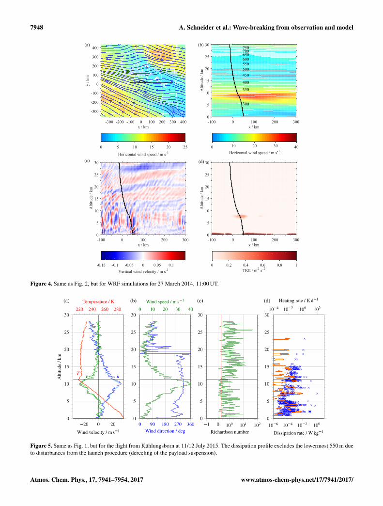
3.3 The 11/12 July 2015 flight

A night-time flight with LITOS was launched from Küh-lungsborn on 11/12 July 2015, at midnight local time(22:01 UT on 11 July). A dereeler of 180 m (with a 3000 gballoon) was used for payload suspension, making balloonwake effects negligible for this flight. The radiosonde waspositioned 60 m below the main payload to avoid distur-bances of the temperature sounding.

The observed background parameters are depicted inFig. 5a and b. Westerly winds prevailed up to ∼ 19 kmaltitude, whereas above winds came from the east. Thischange in direction was not associated with a significantwind shear because velocities were small in that altituderegion. A jet is visible at about 10 km height. Superposedon the winds are signatures of small-scale gravity waves.Above the tropopause at 11.3 km altitude there was a smalltropopause inversion layer. Higher up temperatures remainedrather constant up to∼ 20 km, where they started to increase.

Richardson numbers were typically lower than for theother flights, indicating less stability. There are several lay-ers where the Richardson number is below the critical limitof Ric (1/4). These layers are relatively thin.

Energy dissipation rates (data below 550 m are excludeddue to disturbances from the launch procedure) showed astrong patchy structure, with enhanced dissipation at, for ex-ample, ∼ 2.0, 3.8, 7.2, 8.9, 11.0, 12.1, and 14.3 km. Theselayers of intense turbulence mostly corresponded to Richard-son numbers smaller than Ric = 1/4, or at least to Ri < 1.But particularly in the lower stratosphere between 11 and15 km, turbulence also occurred for high Richardson num-bers. It should be kept in mind that the Richardson numberdepends on the scale on which it is computed (e.g. Balsleyet al., 2008; Haack et al., 2014). A higher resolution (i.e.computingRi on smaller scales) may result in locally smallerRi numbers, because the computation on large scales yieldsa kind of average. Similarly, in large eddy simulations Paoliet al. (2014) found larger Richardson numbers for smallermodel resolutions (i.e. larger scales). Here, due to measure-ment noise a smoothing over 150 m has been applied be-fore computingRi, determining the resolution. However, thisissue cannot explain the whole discrepancy. In simulationsof gravity waves, Achatz (2005) found instabilities and on-set of turbulence for Richardson numbers both smaller andlarger than 1/4. He noted that the theory by Miles (1961)and Howard (1961) is not applicable to his simulations be-cause the gravity wave phase propagation and thus the wave-induced shear is slanted. In the real atmosphere, waves usu-ally propagate at a tilt (i.e. the shear is not orthogonal to thealtitude axis). Hines (1988) has already discussed slantwisestatic instabilities created by gravity waves. He developed

www.atmos-chem-phys.net/17/7941/2017/ Atmos. Chem. Phys., 17, 7941–7954, 2017

7948 A. Schneider et al.: Wave-breaking from observation and model

x / km-300 -200 -100 0 100 200 300 400

y / k

m

-300

-200

-100

0

100

200

300

400

Horizontal wind speed / m s-10 5 10 15 20 25

x / km-100 0 100 200 300

Alti

tude

/ km

0

5

10

15

20

25

30

300

350

400

450500550600650700750

0 10 20 30Horizontal wind speed / m s-1

40

x / km-100 0 100 200 300

Alti

tude

/ km

0

5

10

15

20

25

30

Vertical wind velocity / m s-1-0.15 -0.1 -0.05 0 0.05 0.1

x / km-100 0 100 200 300

Alti

tude

/ km

0

5

10

15

20

25

30

TKE / m2 s-20 0.2 0.4 0.6 0.8 1

(a) (b)

(c) (d)

Figure 4. Same as Fig. 2, but for WRF simulations for 27 March 2014, 11:00 UT.

100 101 102

Richardson number

−1 00

5

10

15

20

25

30

0 90 180 270 3600

5

10

15

20

25

30

Wind direction / deg

0 10 20 30 40

Wind speed / m s−1

−20 0 200

5

10

15

20

25

30

uv

Wind velocity / m s−1

Alti

tude

/km

220 240 260 280

T

Temperature / K

10−4 10−2 100 102

Heating rate / K d−1

10−6 10−4 10−2 1000

5

10

15

20

25

30

Dissipation rate / W kg−1

(a) (b) (c) (d)

Figure 5. Same as Fig. 1, but for the flight from Kühlungsborn at 11/12 July 2015. The dissipation profile excludes the lowermost 550 m dueto disturbances from the launch procedure (dereeling of the payload suspension).

Atmos. Chem. Phys., 17, 7941–7954, 2017 www.atmos-chem-phys.net/17/7941/2017/

A. Schneider et al.: Wave-breaking from observation and model 7949

x / km-300 -200 -100 0 100 200 300 400

y / k

m

-300

-200

-100

0

100

200

300

400

Horizontal wind speed / m s -10 5 10 15 20 25

x / km-100 0 100 200 300

Alti

tude

/ km

0

5

10

15

20

25

30

300 300

350 350

400 400450 450500 500550 550600 600650 650700 700750 750800 800

0 10 20 30 Horizontal wind speed / m s -1

40

x / km-100 0 100 200 300

Alti

tude

/ km

0

5

10

15

20

25

30

Vertical wind velocity / m s-1-0.15 -0.1 -0.05 0 0.05 0.1 0.15

x / km-100 0 100 200 300

Alti

tude

/ km

0

5

10

15

20

25

30

TKE / m2 s-20 0.2 0.4 0.6 0.8 1

(a) (b)

(c) (d)

Figure 6. Same as Fig. 2, but for WRF simulations for 11 July 2015, 23:00 UT.

a wave period criterion for turbulence by comparing the e-folding time of the (slantwise) instability with the period ofthe wave. Turbulence is more likely to occur for slantwisestatic instability than for vertical static instability. In the lightof these comments, the violation of the Richardson criterionfor the LITOS measurements is comprehensible.

Above ∼ 15 km altitude, hardly any turbulence was de-tected; only a few thin turbulent layers were observed. Thusabove 15 km the average dissipation rate (for which no tur-bulence is counted as zero) was only 0.01 mWkg−1, whilebelow 15 km it was 0.64 mWkg−1.

Results from corresponding WRF simulations are depictedin Fig. 6. Horizontal winds at the 850 hPa level were mainlywesterly. The altitude section shows that the strong jet didnot have much variation in the horizontal direction. Verti-cal winds reveal wave patterns that are particularly intensearound the tropopause and gradually become weaker near∼ 15 km, with less amplitude above. This drop in wave am-plitude is at the same altitude as the drop in observed dissipa-tion. The TKE has enlarged values around 3 km altitude andnear the tropopause; however the enhancement is small at the

flight path. Correspondingly, the thickness of the strong tur-bulent layers detected by LITOS is relatively small, meaningthat these dissipative layers are potentially not resolved in themodel.

4 Discussion

A comparison of the observed dissipation profiles and thewave patterns in the model vertical winds for the differentflights suggests that more turbulence observed by LITOScomes along with stronger wave patterns visible in WRF, andvice versa. Particularly, this can be seen at 11/12 July 2015at the drop in dissipation and wave amplitude at ∼ 15 km al-titude. A similar feature has been observed during anotherflight at 6 June 2014 (not shown). Likewise, LITOS data ex-hibit a sharp drop in turbulence at ∼ 15 km, and the corre-sponding WRF simulation shows strong wave patterns below∼ 15 km and very weak ones above. For the troposphere, ver-tical winds in WRF show similar gravity wave amplitudes forall Kühlungsborn soundings, even if the wave structures are

www.atmos-chem-phys.net/17/7941/2017/ Atmos. Chem. Phys., 17, 7941–7954, 2017

7950 A. Schneider et al.: Wave-breaking from observation and model

different. Accordingly, dissipation rates are generally similar,showing up as a highly structured profile that is partly relatedto shear instabilities measured by the radiosonde. This is alsoreflected in the WRF turbulent kinetic energy, attesting thatthe structures are sufficiently large to be resolved in WRF.The same is true for the turbulent layer below the tropopauseobserved during BEXUS 12.

The relation between waves and turbulence can also beseen in averages over altitude regions. For 12 July 2015the most significant drop in mean dissipation does not hap-pen at the tropopause where the stability increases due tothe changing temperature gradient, but at ∼ 15 km wherethe wave activity decreases. Mean energy dissipation ratesare 0.64 mWkg−1 below 15 km altitude and 0.01 mWkg−1

above. Consistent with these rates, the average absolute ver-tical flux calculated from WRF data as a measure for waveactivity is 64 mWm−2 below 15 km and 6.9 mWm−2 above.

We interpret this behaviour as the effect of wave satu-ration. As described in the introduction, a saturated wavelooses part of its energy to turbulence so that the amplitudedoes not grow further. Such effects have already been ob-served, for example, by Cot and Barat (1986), who measureda gravity wave with almost constant amplitude over an alti-tude range of 5 km and collocated isolated turbulent patcheswith a dissipation rate approximately accounting for the en-ergy loss of the wave. Franke and Collins (2003) found re-gions of strong overturning, and upwards-propagating wavesare present below as well as (with less amplitude) above theoverturning region. They argue that, depending on the ampli-tude, a breaking wave is not always completely annihilated,but the amplitude may be modulated in a highly non-linearevent. Nappo (2002, p. 125) states that “gravity wave and tur-bulence are often observed to exist simultaneously.” Via theprocess of wave saturation, the occurrence of waves is con-nected to the intensity of turbulence. Pavelin et al. (2001) ob-served intense turbulence in the lowermost stratosphere dur-ing a period of maximal wave intensity using radar at Aberys-twyth (52.4◦ N, 4.0◦W), which supports the above hypothe-sis.

Saturation theories proposed several mechanisms, e.g. lin-ear instability dynamics due to large wave amplitudes, non-linear damping, or non-linear wave–wave interactions (Frittsand Alexander, 2003, Sect. 6.3). The present study cannot an-swer that debate, yet the relatively large Richardson numbershint that non-linear interactions may play a role.

Mean dissipation rates observed by LITOS are of the or-der of 10−4 Wkg−1 (roughly 0.01 Kd−1). This is 2 ordersof magnitude below typical solar or chemical heating rateswhich are of the order of 1 Kd−1 (Brasseur and Solomon,1986, Fig. 4.19b). However, within thin layers rates of 10−2

to 10−1 Wkg−1 (∼ 1 to 10 Kd−1) are observed, which islarger than solar heating. The low mean energy dissipationrates are not explicitly contained even in high-resolutionmodels, which cannot describe the large intermittency. Only

large layers with highly increased dissipation, as encoun-tered, for example, during BEXUS 12, are captured.

Observed dissipation rates are partly larger than thosereported by other publications using different methods.Barat (1982) obtained values between 1.4× 10−5 and 3.9×10−5 Wkg−1 from balloon measurements. Wilson et al.(2014) found ε values between 3×10−5 and 6×10−4 Wkg−1

in the upper troposphere from radar measurements. Theseare lower rates than the averages in this work, but withinthe range of the variability. Lilly et al. (1974) observedstratospheric dissipation rates between 7× 10−4 and 2×10−3 Wkg−1, depending on the underlying terrain, with anaircraft. These results are of a similar order of magnitude tothe averages in this study. Haack et al. (2014) reported meandissipation rates between 2× 10−2 and 5× 10−3 Wkg−1 forthe altitude range 7 to 26.5 km, using a different retrieval andpotentially including wake effects.

5 Conclusions

In this paper, high-resolution turbulence observations withLITOS are complemented by model simulations with WRFto study the relation between turbulence, waves, and back-ground conditions. Three flights, for which in each case datafrom two wind sensors are available, are selected. This allowshigh-quality assurance. Furthermore, any data that are possi-bly influenced by the balloon’s wake have been removed forthis study.

Enhanced energy dissipation rates were observed wherepronounced instabilities were detected by the radiosonde.Moreover, measured shear instabilities and associated en-hancements in dissipation on scales resolved by WRFalso coincide with enlarged model turbulent kinetic en-ergy (TKE). For instance, during the BEXUS 12 flight(27 September 2011), a wind reversal was observed whichcaused a large shear instability (indicated by Richardsonnumbers smaller than 1/4) as well as potential wave filter-ing. The resulting turbulence was detected by LITOS as aregion with large dissipation rates. The model TKE peaksin this region, highlighting the significance of that layer.Similar effects are observed for some strong layers of the27 March 2014 and 11/12 July 2015 flights. Thus, in thesecases the geophysical causes of the observed turbulent layersare clearly visible. The large scale instabilities are resolvedby the radiosondes and the model. On the other hand, manyother (less intense) turbulent layers observed by LITOS areobviously too thin to be related to the much coarser data ofthe radiosonde or the WRF results.

Another relation between turbulence detected by LITOSand the presence of wave-like structures in WRF is noted:for the available summer flights at 6 June 2014 (not shown)and 12 July 2015, a drop in turbulence occurrence at ap-proximately 15 km altitude with hardly any turbulence abovewas observed. In the associated model simulations, wave sig-

Atmos. Chem. Phys., 17, 7941–7954, 2017 www.atmos-chem-phys.net/17/7941/2017/

A. Schneider et al.: Wave-breaking from observation and model 7951

natures become weaker around 15 km. Altogether, observeddissipation is weaker during lower wave activity (as seen inWRF), and larger where larger wave amplitudes are seen.These findings can be explained by wave saturation, whilea change in, for example, static stability is less prominent.

Turbulence has been observed for Richardson numbers be-low as well as above the critical number of 1/4, partly evenfor values much larger than 1. Such a violation of the clas-sical theory by Miles (1961) and Howard (1961) has alreadybeen described by several researchers, e.g. Achatz (2005);Galperin et al. (2007); Balsley et al. (2008). Hines (1988)recognised the limitation of considering only vertical insta-bility (as done when using the Richardson number) and pro-posed a concept of slantwise instabilities as created by grav-ity waves. He showed that turbulence is more likely to de-

velop via slanted instability compared to vertical instability.Thus turbulence for Ri > 1/4 is comprehensible.

The results are based on the limited data set from a fewflights. More flights at selected meteorological situations areplanned to further study the relation between waves and tur-bulence. A redesign of the instrumental set-up shall elimi-nate the wake effects of balloon and ropes. Moreover, a di-rect measurement of gravity wave activity in combination tothe turbulence observations is preferable.

Data availability. The data used in this study are available on re-quest to Michael Gerding (gerding@iap-kborn.de).

www.atmos-chem-phys.net/17/7941/2017/ Atmos. Chem. Phys., 17, 7941–7954, 2017

7952 A. Schneider et al.: Wave-breaking from observation and model

Appendix A: Derivation of the constant cl0 in Eq. (1)

To retrieve energy dissipation rates from observed spectra,the relation (Eq. 1) between inner scale l0 and dissipationrate ε, ε = c4

l0ν3/l40 , and especially the value of the constant

cl0 is important. To obtain correct values, care has to be takenas which component(s) of the spectral tensor are observed.In the following, the derivation of the constant cl0 is sum-marised.

In the inertial subrange, the longitudinal component,transversal component, and trace of the structure functiontensor for velocity fluctuations have the form

Dxx(r)= Cxxr2/3, (A1)

where xx is a placeholder for rr (longitudinal), tt (transver-sal), or ii (trace), and the structure constant has the formCxx = bxxa

2vε

2/3 with brr = 1, btt =43 , bii = brr+ 2btt =

113

(Tatarskii, 1971, p. 54ff) and the empirical constant a2v = 2.0

(e.g. Pope, 2000, p. 193f). In the viscous subrange, the struc-ture function is

Dxx(r)= C̃xxr2, (A2)

with C̃xx = cxxεν

and the factors crr =1

15 , ctt =2

15 , cii =crr+ 2ctt =

13 (Tatarskii, 1971, p. 49).

Based on Heisenberg (1948, Eq. 28), Lübken and Hillert(1992, Eq. 4) gave a form of the temporal spectrum in the in-ertial and viscous subranges, which reads, for velocity fluc-tuations,

W(ω)=0( 5

3 )sin(π3 )2πub

Cxx(ω/ub)

−5/3(1+

(ω/ubk0

)8/3)2 , (A3)

where ub is the ascent velocity of the balloon, 0(z) :=∫∞

0 tz−1e−t dt is the gamma function, and k0 denotes thebreakpoint between inertial and viscous subrange. The nor-malisation is obtained by considering the limit k� k0 for the

inertial subrange. Using the relation 8(k)=− u2b

2πkdWdω (kub)

between temporal and spatial spectrum (Tatarskii, 1971,Eq. 6.14), the corresponding three-dimensional spectrum is

8xx(k)= (A4)

16π

0( 53 )sin(π3 )

2πCxx k

−11/35+ 21

(kk0

)8/3

(1+

(kk0

)8/3)3 .

The constant cl0 in Eq. (1) can be computed from the condi-tion of the structure function at the origin

d2Dxx

dr2 (0)=8π3

∞∫0

8xx(k)k4 dk (A5)

(Tatarskii, 1971, p. 49f). Inserting the structure function(Eq. A2) and the spectrum (Eq. A4) into condition (Eq. A5),integrating and solving for 1/k0 yields

l0 =2πk0

(A6)

= 2π(

3160(5/3)sin(π/3)

bxx

cxxa2

v

)3/4

︸ ︷︷ ︸=cl0

(ν3

ε

)1/4

.

CTA wire probes are sensitive perpendicular to the wireaxis but insensitive parallel to the wire axis. For the earlierflights, the wires of the CTA sensors were oriented verticallyso that they are sensitive in both horizontal directions andinsensitive in the vertical direction; i.e. for an ascending bal-loon both transversal components are measured. Thus bxx =4/3+4/3= 8/3 and cxx = 2/15+2/15= 4/15, which leadsto cl0 = 14.1. For the flight at 12 July 2015, one sensor withthe wire oriented horizontally was flown, which is sensitivein the vertical and one horizontal direction yet insensitive inthe other horizontal direction (parallel to the wire). In thiscase bxx = 1+ 4/3= 7/3 and cxx = 1/15+ 2/15= 3/15 sothat cl0 = 15.8.

Haack et al. (2014, Sect. 4) used different components ofthe structure function constant yielding cl0 = 5.7. Since inEq. (1) the constant occurs with c4

l0, this results in a difference

in ε of a factor of ∼ 50 for the same l0.

Atmos. Chem. Phys., 17, 7941–7954, 2017 www.atmos-chem-phys.net/17/7941/2017/

A. Schneider et al.: Wave-breaking from observation and model 7953

Competing interests. The authors declare that they have no conflictof interest.

Acknowledgements. The BEXUS programme was financed by theGerman Aerospace Center (DLR) and the Swedish National SpaceBoard (SNSB). We are grateful for the support from the Interna-tional Leibniz Graduate School for Gravity Waves and Turbulencein the Atmosphere and Ocean (ILWAO) funded by the LeibnizAssociation (WGL). This study was partly funded by the GermanFederal Ministry for Education and Research (BMBF) researchinitiative “Role of the Middle Atmosphere In Climate” (ROMIC)under project numbers 01LG1206A and 01LG1218A (METROSI),and by the German Research Foundation (DFG) under projectnumbers LU 1174 (PACOG) and FOR 1898 (MS-GWaves). Wethank Wayne K. Hocking and two anonymous reviewers for theirvaluable comments leading to the improvement of this article. Thepublication of this article was funded by the Open Access Fund ofthe Leibniz Association.

Edited by: Peter HaynesReviewed by: Wayne K. Hocking and two anonymous referees

References

Achatz, U.: On the role of optimal perturbations in the instabil-ity of monochromatic gravity waves, Phys. Fluids, 17, 094107,https://doi.org/10.1063/1.2046709, 2005.

Andreassen, O., Wasberg, C. E., Fritts, D. C., and Isler, J. R.: Grav-ity wave breaking in two and three dimensions: 1. Model descrip-tion and comparison of two-dimensional evolutions, J. Geophys.Res., 99, 8095–8108, https://doi.org/10.1029/93JD03435, 1994.

Balsley, B. B., Svensson, G., and Tjernström, M.: On theScale-dependence of the Gradient Richardson Number inthe Residual Layer, Bound.-Lay. Meteorol., 127, 57–72,https://doi.org/10.1007/s10546-007-9251-0, 2008.

Barat, J.: Some characteristics of clear-air tur-bulence in the middle stratosphere, J. Atmos.Sci., 39, 2553–2564, https://doi.org/10.1175/1520-0469(1982)039<2553:SCOCAT>2.0.CO;2, 1982.

Barat, J., Cot, C., and Sidi, C.: On the measurement of turbulencedissipation rate from rising balloons, J. Atmos. Ocean. Tech., 1,270–275, 1984.

Birner, T.: Fine-scale structure of the extratropicaltropopause region, J. Geophys. Res., 111, D04104,https://doi.org/10.1029/2005JD006301, 2006.

Birner, T., Dörnbrack, A., and Schumann, U.: How sharp is thetropopause at midlatitudes?, Geophys. Res. Lett., 29, 45-1–45-4, https://doi.org/10.1029/2002GL015142, 2002.

Brasseur, G. and Solomon, S.: Aeronomy of the middle atmosphere:chemistry and physics of the stratosphere and mesosphere, 2ndEdn., Atmospheric sciences library, Reidel, Dordrecht, 1986.

Chen, F. and Dudhia, J.: Coupling an Advanced Land Surface–Hydrology Model with the Penn State-NCAR MM5 Mod-eling System, Part I: Model Implementation and Sensitivity,Mon. Weather Rev., 129, 569–585, https://doi.org/10.1175/1520-0493(2001)129<0569:CAALSH>2.0.CO;2, 2001.

Cho, J. Y. N., Newell, R. E., Anderson, B. E., Barrick, J. D. W.,and Thornhill, K. L.: Characterizations of tropospheric turbu-lence and stability layers from aircraft observations, J. Geophys.Res., 108, 8784, https://doi.org/10.1029/2002JD002820, 2003.

Chou, M. D. and Suarez, M. J.: An efficient thermal infrared ra-diation parameterization for use in general circulation models,NASA Tech. Memo., 104606, 85 pp., 1994.

Clayson, C. A. and Kantha, L.: On Turbulence and Mixingin the Free Atmosphere Inferred from High-ResolutionSoundings, J. Atmos. Ocean. Tech., 25, 833–852,https://doi.org/10.1175/2007JTECHA992.1, 2008.

Cot, C. and Barat, J.: Wave-turbulence interaction in the strato-sphere: A case study, J. Geophys. Res., 91, 2749–2756,https://doi.org/10.1029/JD091iD02p02749, 1986.

Dalaudier, F., Sidi, C., Crochet, M., and Vernin, J.: Direct Ev-idence of “Sheets” in the Atmospheric Temperature Field,J. Atmos. Sci., 51, 237–248, https://doi.org/10.1175/1520-0469(1994)051<0237:DEOITA>2.0.CO;2, 1994.

Ehard, B., Achtert, P., Dörnbrack, A., Gisinger, S., Gumbel, J., Kha-planov, M., Rapp, M., and Wagner, J. S.: Combination of li-dar and model data for studying deep gravity wave propagation,Mon. Weather Rev., 144, 77–98, https://doi.org/10.1175/MWR-D-14-00405.1, 2016.

Franke, P. M. and Collins, R. L.: Evidence of gravity wave breakingin lidar data from the mesopause region, Geophys. Res. Lett., 30,https://doi.org/10.1029/2001GL014477, 1155, 2003.

Fritts, D. C. and Alexander, M. J.: Gravity wave dynamics andeffects in the middle atmosphere, Rev. Geophys., 41, 1003,https://doi.org/10.1029/2001RG000106, 2003.

Fritts, D. C. and Wang, L.: Gravity Wave–Fine Structure In-teractions, Part II: Energy Dissipation Evolutions, Statis-tics, and Implications, J. Atmos. Sci., 70, 3735–3755,https://doi.org/10.1175/JAS-D-13-059.1, 2013.

Fritts, D. C., Wang, L., Geller, M. A., Lawrence, D. A., Werne, J.,and Balsley, B. B.: Numerical Modeling of Multiscale Dynam-ics at a High Reynolds Number: Instabilities, Turbulence, and anAssessment of Ozmidov and Thorpe Scales, J. Atmos. Sci., 73,555–578, https://doi.org/10.1175/JAS-D-14-0343.1, 2016.

Galperin, B., Sukoriansky, S., and Anderson, P. S.: On the criticalRichardson number in stably stratified turbulence, Atmos. Sci.Lett., 8, 65–69, https://doi.org/10.1002/asl.153, 2007.

Gavrilov, N. M.: Estimates of turbulent diffusivities and energydissipation rates from satellite measurements of spectra ofstratospheric refractivity perturbations, Atmos. Chem. Phys.,13, 12107–12116, https://doi.org/10.5194/acp-13-12107-2013,2013.

Haack, A., Gerding, M., and Lübken, F.-J.: Characteristics of strato-spheric turbulent layers measured by LITOS and their relation tothe Richardson number, J. Geophys. Res., 119, 10605–10618,https://doi.org/10.1002/2013JD021008, 2014.

Hauf, T.: Aircraft Observation of Convection Waves overSouthern Germany – A Case Study, Mon. WeatherRev., 121, 3282–3290, https://doi.org/10.1175/1520-0493(1993)121<3282:AOOCWO>2.0.CO;2, 1993.

Heisenberg, W.: Zur statistischen Theorie der Turbulenz, Z. Phys.,124, 628–657, https://doi.org/10.1007/BF01668899, 1948.

Hines, C. O.: Generation of Turbulence by At-mospheric Gravity Waves, J. Atmos. Sci.,

www.atmos-chem-phys.net/17/7941/2017/ Atmos. Chem. Phys., 17, 7941–7954, 2017

7954 A. Schneider et al.: Wave-breaking from observation and model

45, 1269–1278, https://doi.org/10.1175/1520-0469(1988)045<1269:GOTBAG>2.0.CO;2, 1988.

Hines, C. O.: The Saturation of Gravity Waves in the Mid-dle Atmosphere, Part I: Critique of Linear-Instability Theory,J. Atmos. Sci., 48, 1348–1360, https://doi.org/10.1175/1520-0469(1991)048<1348:TSOGWI>2.0.CO;2, 1991.

Hocking, W. K.: A review of Mesosphere–Stratosphere–Troposphere (MST) radar developments and studies,circa 1997–2008, J. Atmos. Sol.-Terr. Phy., 73, 848–882,https://doi.org/10.1016/j.jastp.2010.12.009, 2011.

Hodges, R. R.: Generation of turbulence in the upper atmosphereby internal gravity waves, J. Geophys. Res., 72, 3455–3458,https://doi.org/10.1029/JZ072i013p03455, 1967.

Hong, S.-Y. and Lim, J.-O. J.: The WRF single-moment 6-class mi-crophysics scheme (WSM6), J. Korean Meteor. Soc., 42, 129–151, 2006.

Howard, L. N.: Note on a paper of John W. Miles, J. Fluid Mech.,10, 509–512, https://doi.org/10.1017/S0022112061000317,1961.

Kain, J. S. and Fritsch, J. M.: A One-DimensionalEntraining/Detraining Plume Model and Its Appli-cation in Convective Parameterization, J. Atmos.Sci., 47, 2784–2802, https://doi.org/10.1175/1520-0469(1990)047<2784:AODEPM>2.0.CO;2, 1990.

Klemp, J. B., Dudhia, J., and Hassiotis, A. D.: An Up-per Gravity-Wave Absorbing Layer for NWP Ap-plications, Mon. Weather Rev., 136, 3987–4004,https://doi.org/10.1175/2008MWR2596.1, 2008.

Lilly, D. K., Waco, D. E., and Adelfang, S. I.: Stratospheric Mix-ing Estimated from High-Altitude Turbulence Measurements,J. Appl. Meteor., 13, 488–493, https://doi.org/10.1175/1520-0450(1974)013<0488:SMEFHA>2.0.CO;2, 1974.

Lindzen, R. S.: Turbulence and stress owing to gravity waveand tidal breakdown, J. Geophys. Res., 86, 9707–9714,https://doi.org/10.1029/JC086iC10p09707, 1981.

Lübken, F.-J. and Hillert, W.: Measurements of turbulent energy dis-sipation rates applying spectral models, in: Coupling Processesin the Lower and Middle Atmosphere, NATO Advanced Re-search Workshop, Kluwer Press, Loen, Norway, 345–351, 1992.

Luce, H., Fukao, S., Dalaudier, F., and Crochet, M.: StrongMixing Events Observed near the Tropopause with theMU Radar and High-Resolution Balloon Techniques, J.Atmos. Sci., 59, 2885–2896, https://doi.org/10.1175/1520-0469(2002)059<2885:SMEONT>2.0.CO;2, 2002.

Miles, J. W.: On the stability of heterogeneousshear flows, J. Fluid Mech., 10, 496–508,https://doi.org/10.1017/S0022112061000305, 1961.

Mlawer, E. J., Taubman, S. J., Brown, P. D., Iacono, M. J.,and Clough, S. A.: Radiative transfer for inhomoge-neous atmospheres: RRTM, a validated correlated-k modelfor the longwave, J. Geophys. Res., 102, 16663–16682,https://doi.org/10.1029/97JD00237, 1997.

Nakanishi, M. and Niino, H.: Development of an Improved Tur-bulence Closure Model for the Atmospheric Boundary Layer,J. Meteor. Soc. Japan, 87, 895–912, http://ci.nii.ac.jp/naid/110007465760/en/, 2009.

Nappo, C. J.: An Introduction to Atmospheric Gravity Waves, Inter-national Geophysics Series, Academic Press, San Diego, Vol. 85,2002.

Osman, M., Hocking, W., and Tarasick, D.: Parameterization oflarge-scale turbulent diffusion in the presence of both well-mixedand weakly mixed patchy layers, J. Atmos. Sol.-Terr. Phy., 143–144, 14–36, https://doi.org/10.1016/j.jastp.2016.02.025, 2016.

Paoli, R., Thouron, O., Escobar, J., Picot, J., and Cariolle,D.: High-resolution large-eddy simulations of stably stratifiedflows: application to subkilometer-scale turbulence in the uppertroposphere–lower stratosphere, Atmos. Chem. Phys., 14, 5037–5055, https://doi.org/10.5194/acp-14-5037-2014, 2014.

Pavelin, E., Whiteway, J. A., and Vaughan, G.: Observa-tion of gravity wave generation and breaking in the low-ermost stratosphere, J. Geophys. Res., 106, 5173–5179,https://doi.org/10.1029/2000JD900480, 2001.

Pope, S. B.: Turbulent Flows, Cambridge University Press, Cam-bridge, 2000.

Schneider, A., Gerding, M., and Lübken, F.-J.: Compar-ing turbulent parameters obtained from LITOS and ra-diosonde measurements, Atmos. Chem. Phys., 15, 2159–2166,https://doi.org/10.5194/acp-15-2159-2015, 2015.

Skamarock, W. C., Klemp, J. B., Dudhia, J., Gill, D. O., Barker,D. M., Duda, M. G., Huang, X.-Y., Wang, W., and Powers,J. G.: A description of the Advanced Research WRF Version3, NCAR technical note, Mesoscale and Microscale Meteo-rology Division, National Center for Atmospheric Research,Boulder, Colorado, USA, http://www2.mmm.ucar.edu/wrf/users/docs/arw_v3.pdf, 2008.

Tatarskii, V. I.: The effects of the turbulent atmosphere onwave propagation, Israel Program for Scientific Translations,Jerusalem, translated from Russian, 1971.

Theuerkauf, A., Gerding, M., and Lübken, F.-J.: LITOS – anew balloon-borne instrument for fine-scale turbulence sound-ings in the stratosphere, Atmos. Meas. Tech., 4, 55–66,https://doi.org/10.5194/amt-4-55-2011, 2011.

Wilson, R.: Turbulent diffusivity in the free atmosphere inferredfrom MST radar measurements: a review, Ann. Geophys., 22,3869–3887, https://doi.org/10.5194/angeo-22-3869-2004, 2004.

Wilson, R., Luce, H., Hashiguchi, H., Nishi, N., and Yabuki,Y.: Energetics of persistent turbulent layers underneathmid-level clouds estimated from concurrent radar andradiosonde data, J. Atmos. Sol.-Terr. Phy., 118, 78–89,https://doi.org/10.1016/j.jastp.2014.01.005, 2014.

Worthington, R. M.: Tropopausal turbulence caused by the breakingof mountain waves, J. Atmos. Sol.-Terr. Phys., 60, 1543–1547,https://doi.org/10.1016/S1364-6826(98)00105-9, 1998.

Yamanaka, M. D., Tanaka, H., Hirosawa, H., Matsuzaka, Y., Ya-magami, T., and Nishimura, J.: Measurement of StratosphericTurbulence by Balloon-Borne “Glow-Discharge” Anemometer,J. Meteor. Soc. Japan Ser. II, 63, 483–489, https://www.jstage.jst.go.jp/article/jmsj1965/63/3/63_3_483/_article, 1985.

Atmos. Chem. Phys., 17, 7941–7954, 2017 www.atmos-chem-phys.net/17/7941/2017/