tr cerc-93-11, nearshore wave breaking and decay

US Army Corps of Engineers Waterways Experiment Station

Nearshore Wave Breaking and Decay

by Jane M. Smith Coastal Engineering Research Center

Approved For Public Release; Distribution Is Unlimited

Prepared for Headquarters, U.S. Army Corps of Engineers

Technical Report CERC-93-11 July 1993

o

The contents of this report are not to be used for advertising, publication, or promotional purposes. Citation of trade names does not constitute an official endorsement or approval of the use of such commercial products.

PRINTED ON RECYCLED PAPER

Nearshore Wave Breaking and Decay by Jane M. Smith

Coastal Engineering Research Center

U.S. Army Corps of Engineers Waterways Experiment Station 3909 Halls Ferry Road Vicksburg, MS 39180-6199

Final report

Approved for public release; distribution is unlimited

Prepared for U.S. Army Corps of Engineers Washington, DC 20314-1000

Technical Report CERC-93-11 July 1993

US Army Corps of Engineers Waterways Experiment Station

Fa:11NFOA1M11OH CONTACT:

PUBUC AFFAIRS OFRCE U. S. ARMY ENGINEER

N

WATERWAYS EXPERIMENT STAllON _ HALUI FERRY ROAII

VICKSBURG, .. S8IS8IPPI 311180-61118 PHONE: Ceo1)634-2!02

... N1EA OF REBEFN'A11ON. UIq 11m

Waterways Experiment Station Cataloging-in-Publication Data

Smith. Jane M.

&aim

I

Nearshore wave breaking and decay / by Jane M. Smith. Coastal Engineer~ ing Research Center; prepared for U.S. Army Corps of Engineers.

53 p. : ill. ; 28 cm. - (Technical report; CERC-93-11) Includes bibliographical references. 1. Ocean waves - Mathematical models. 2. Water waves. 3. Hydrody

namics. I. United States. Army. Corps of Engineers. II.. Coastal Engineering Research Center (U.S.) III. U.S. Army Engineer Waterways Experiment Station. IV. Title. V. Series: Technical report (U.S. Army Engineer Waterways Experiment Station) ; CERC-93-11. TA7 W34 no.CERC-93-11

Contents

Preface .......................................... v

I-Introduction ..................................... 1

Background . . . . . . . . . . . . . . . . . . . . . . . . . . . . . . . . . . . . .. 1 Scope ......................................... 1

2-Incipient Wave Breaking ............................. 3

Breaker Type . . . . . . . . . . . . . . . . . . . . . . . . . . . . . . . . . . . .. 3 Breaker Index .................................... 4

3-Surf Zone Wave Transformation ........................ 9

Regular Waves . . . . . . . . . . . . . . . . . . . . . . . . . . . . . . . . . . .. 9 Similarity method . . . . . . . . . . . . . . . . . . . . . . . . . . . . . . .. 9 Energy flux method . . . . . . . . . . . . . . . . . . . . . . . . . . . . . .. 11

Irregular Waves .... . . . . . . . . . . . . . . . . . . . . . . . . . . . . . .. 12 Statistical approaches . . . . . . . . . . . . . . . . . . . . . . . . . . . . . . 12 Spectral approaches ............................... 14

4-Wave Attenuation Over Reefs .......................... 17

Wave Processes ................................... 17 Wave breaking . . . . . . . . . . . . . . . . . . . . . . . . . . . . . . . . .. 17 Breaker models ................................. 18

Modeling Methodology .............................. 19 Sample Results. . . . . . . . . . . . . . . . . . . . . . . . . . . . . . . . . . .. 19 Recommendations . . . . . . . . . . . . . . . . . . . . . . . . . . . . . . . . . . 20

5-Shoaling and Decay of MUltiple Wave Trains ................ 24

Laboratory Experiments . . . . . . . . . . . . . . . . . . . . . . . . . . . . . . 24 Wave Spectra .................................... 25 Wave Heights .................................... 28 Summary ....................................... 30

6--Conclusions ..................................... 31

iii

iv

References ........................................ 32

Appendix A: Agat Laboratory Wave Measurements ............. Al

Appendix B: Notation...... . . . . . . . . . . . . . . . . . . . . . . . . .. Bl

SF 298

List of Figures

Figure 1. Breaker depth index as a function of H/(g T2) ........... 6

Figure 2. Breaker depth index as a function of HJLo . . . . . . . . . . . . .. 6

Figure 3. Change in wave profile shape from outside the surf zone to inside the surf zone . . . . . . . . . . . . . . . . . . . . . . . . . . . . . . . . . . . . . .. 10

Figure 4. Example NMLONG simulation of wave height transformation, Leadbetter Beach, California, 3 Feb 1980 . . . . . . . . . . . . . . . . . . . . . 13

Figure 5. Example NMLONG simulation of wave height transformation, Duck, North Carolina, 14 Oct 1990 ......................... 13

Figure 6. Shallow-water wave spectra . . . . . . . . . . . . . . . . . . . . . . . 15

Figure 7. Laboratory test 18, Agat, Guam .................... 21



Figure 10. Calculated versus measured laboratory results ........... 22

Figure 11. Field test, August 1985, Yonge Reef, Australia .......... 23

Figure 12. Energy spectra for 1'" = 2.5/1.25 sec, Hmo = 15.2 cm ..... 25

Figure 13. Energy spectra for 1'" = 2.5/1.25 sec, Hmo = 15.2 cm ..... 26

Figure 14. Energy spectra for 1'" = 2.5/1.75 sec, Hmo = 9.2 em ...... 26

Figure 15. Energy spectra for 1'" = 2.5/1.75 sec, Hmo = 9.2 em ...... 27

Figure 16. H1I3 versus mean water depth ..................... 29

Figure 17. Hmo versus mean water depth ..................... 29

Preface

The work described in this report was authorized as part of the Civil Works Research and Development Program by Headquarters, U.S. Army Corps of Engineers (HQUSACE). This report summarizes wave breaking investigations performed under Work Unit 31672, "Nearshore Waves and Currents," at the Coastal Engineering Research Center (CERC) of the U.S. Army Engineer Waterways Experiment Station (WES). Messrs. John H. Lockhart, Jr., John G. Housley, Barry W. Holliday, and David A. Roellig were HQUSACE Technical Monitors. Ms. Carolyn M. Holmes was the CERC Program Manager.

This study was conducted from September 1992 through March 1993 by Ms. Jane McKee Smith, Research Hydraulic Engineer, CERC. The study was done under the general supervision of Dr. James R. Houston and Mr. Charles C. Calhoun, Jr., Director and Assistant Director, CERC, respectively; and under the direct supervision of Mr. H. Lee Butler, Chief, Research Division, and Mr. Bruce A. Ebersole, Chief, Coastal Processes Branch, CERC. Laboratory measurements of waves on reefs and breaking of multiple wave trains were made by Messrs. John M. Heggins and Donald L. Ward, Wave Research Branch, CERC, respectively. Ms. Mary A. Cialone, Mr. W. Gray Smith, and Mr. Bruce A. Ebersole, Coastal Processes Branch, CERC, provided technical review of this report.

Dr. Robert W. Whalin was Director of WES. COL Leonard G. Hassell, EN, was Commander.

v

1 Introduction

Background

Waves approaching the coast increase in steepness as the water depth decreases. When the wave height is approximately equal to the water depth, the wave breaks, dissipating wave energy and inducing longshore currents and an increase in the mean water level. The sUrf zone is the region from shoreline to the seaward boundary of wave breaking. Within the surf zone, wave breaking is the dominant feature. The surf zone is the most dynamic coastal region with sediment transport and bathymetry change driven by breaking waves and wave-induced currents.

Surf zone wave conditions are required for estimating potential storm damage (flooding and wave damage), calculating shoreline evolution and cross-shore beach profile change, designing coastal structures (jetties, groins, seawalls) and beach fills, and developing shoreline management policy. To provide improved estimates of surf zone waves, the Nearshore Waves and Currents Work Unit in the Coastal Flooding and Storm Protection Program developed, validated, and improved the numerical modeling of wave breaking and decay through laboratory experiments and field studies. Areas of research included incipient breaker indices, surf zone wave decay expressions, spectral shapes in the surf zone, wave breaking on reefs, and decay of multiple wave trains.

Scope

The purpose of this report is to summarize the nearshore wave breaking and decay research performed under the Nearshore Waves and Currents Work Unit. Chapter 2 describes incipient wave breaking and breaker types. Also, expressions are given for the breaker depth index and breaker height index. Guidance is given for both regular and irregular waves. The decay in wave height through the surf zone is discussed in Chapter 3. Regular wave methods include the simple constant ratio of wave height to water depth and the energy flux method. Irregular wave methods include statistical and spectral approaches. Chapter 4 applies wave height decay methodology to the special problem of wave breaking on reefs. Reefs have steep offshore slopes and rough, flat reef tops, so the wave characteristics differ from typical sandy beaches.

Chapter 1 Introduction 1

2

Chapter 5 presents results on the decay of multiple wave trains. Generally. more than one wave train exists at a coastal site, but no guidance exists on how to apply wave breaking to multiple wave trains. This chapter discusses laboratory tests on the decay of multiple wave trains.

Chapter 1 Introduction

2 Incipient Wave Breaking

As waves approach a beach, they increase in steepness (ratio of wave height H 1 to wavelength L) -- length decreases and height may increase. Waves break as they reach a limiting steepness which is a function of the relative depth (ratio of the depth d to the wave length) and the beach slope tan {3. Incipient breaking can be defined several ways (Singamsetti and Wind 1980):

a. The point where the wave cannot further adapt to the changing bottom configuration and starts to disintegrate.

b. The point where the horizontal component of the water particle velocity at the crest becomes greater than the wave celerity.

c. The point where the wave height is maximum.

d. The point where part of the wave front becomes vertical.

e. The point where the radiation stresses start to decrease.

f The point where the water particle acceleration at the crest tends to separate the particles from the water surface.

g. The point where the pressure at the free surface given by the Bernoulli equation is incompatible with the atmospheric pressure.

Determination of the incipient break point is subjective since waves generally break gradually.

Breaker Type

Breaker type refers to the form of the wave at breaking. Wave breaking may be classified into four types (Galvin 1968): spilling, plunging, collapsing, and surging. In spilling breakers the wave crest becomes unstable and cascades down the shoreward face of the wave producing a foamy water sur-

1 For convenience, symbols and abbreviations are listed in the notation (Appendix B).

Chapter 2 Incipient Wave Breaking 3

4

cascades down the shoreward face of the wave producing a foamy water surface. In plunging breakers the crest curls over the shoreward face of the wave and falls into the base of the wave, resulting in a high splash. In collapsing breakers the crest remains unbroken while the lower part of the shoreward face steepens and then falls, producing an irregular turbulent water surface. In surging breakers the crest remains unbroken and the front face of the wave advances up the beach with minor breaking.

The surf similarity parameter t .. defined as

(1)

where the subscript 0 denotes deepwater parameters, is used to distinguish breaker type (Galvin 1968, Battjes 1974). The breaker type is estimated by

surging/collapsing for plunging for

spilling for

~o > 3.3 0.5 < ~o < 3.3

~o < 0.5

(2)

As expressed in Equation 2, spilling breakers tend to occur for high-steepness waves on low-slope beaches. Plunging breakers occur on steeper beaches with intermediately steep waves, and surging breakers occur for low steepness waves on steep beaches. Extremely low steepness waves may not break, but instead reflect from the beach, forming a standing wave.

Spilling breakers differ little in fluid motion from unbroken waves (Divoky, LeMQlaute, and Lin 1970) and generate less turbulence near the bottom and thus tend to be less effective in suspending sediment than plunging or collapsing breakers. The most intense local fluid motions are produced by a plunging breaker. As it breaks, the crest of the plunging wave acts as a free-falling jet that scours a trough into the bottom. The transition from one breaker type to another is gradual and without distinct dividing lines. The direction and magnitude of the local wind can affect breaker type. Onshore winds cause waves to break in deeper water depths and spill, while offshore winds cause waves to break in shallower depths and plunge (Galloway, Collins, and Moran 1989; Douglass 1990).

Breaker Index

Many studies have been performed to develop relationships to predict the wave height at incipient breaking. The term breaker index is used to describe nondimensional breaker height. Two common indices are of the form

Hb Yb =

db (3)

Chapter 2 Incipient Wave Breaking

where

'Yh = breaker depth index Hb = wave height at incipient breaking db = mean water depth at incipient breaking

and

(4)

in which Ob is the breaker height index.

Early studies on breaker indices were conducted using solitary waves. McCowan (1891) theoretically determined the breaker depth index as 'Yb = 0.78 for a solitary wave traveling over a horizontal bottom. Munk (1949) derived the expression Ob = 0.3 (HjL)-J/3 for the breaker height index from solitary wave theory. Subsequent studies, based on periodic waves, by Iversen (1952), Goda (1970), Weggel (1972), Singamsetti and Wind (1980), Sunamura (1980), Smith and Kraus (1991), and others have established that breaker indices depend on beach slope and incident wave steepness.

From monochromatic laboratory data on smooth, plane slopes, Weggel (1972) derived the following expression for the maximum breaker depth index

Hb Yb ;;; b - a -

g'fl (5)

for tan {3 ~ 1/10 and HjLo ~ 0.06, where T is wave period, and g is gravitational acceleration. The parameters a and b were empirically determined functions of the beach slope, given by

a ;;; 43.8 (1 - e-19 tan P)

b = __ 1_.5_6 __ (1 + e -19.5 tan P)

(6)

(7)

The breaking wave height Hb is contained on both sides of Equation 5, so the equation must be solved iteratively. Figure 1 graphically shows the breaker depth index dependency on wave steepness and bottom slope (Equation 5).

Smith and Kraus (1991) combined monochromatic laboratory data from Iversen (1952), Horikawa and Kuo (1966), Galvin (1969), Saeki and Sasaki (1973), Iwagaki et al. (1974), Walker (1974), Singamsetti and Wind (1980), Mizuguchi (1980), Maruyama et al. (1983), Visser (1982), and Stive (1985) with data collected in their own experiments to empirically obtain


6

Q:)

~'---~----~---T----r---~--~----~---T----'---I

~~---4~~+----+----~--~---4----+----+----r---~

Q:)

Q~--~----+---~----r---~---4----~---+----~~~ 0.000 0.004 0.008 0.012 0.016 0.020

Hjgr

Figure 1. Breaker depth index as a function of H,/(g T2) (Equation 5) (Weggel 1972)

~'---~----~--~----T----r----r---~--~----~--~

,;,

~~-t----+-~~~~~---t-~~~~~~-t----+----~--~ ,;,0

~

"'" Q-t---~-----t---~----+---~----r---~---4----~--~ 0.00 0.02 0.04 0.06 0.08 0.10

HolLo

Figure 2. Breaker depth index as a function of H.,ILo (Equation 8) (Smith and Kraus 1991)


Y b = 1.12 - 5.0 (1 - e43 tan II) (HLoo)

1 + e-60 am ll (8)

for 0.0007 ~ H/LD ~ 0.0921 and 1180 ~ tan fJ ~ 1/10. Equation 8 is similar in form to Equation 5, but Hb appears only in 'Yb so the equation can be solved without iteration. Equation 8 generally gives values of 'Yb that are approximately 5 to 20 percent smaller than Equation 5 for 1180 ~ tan fJ ~ 1110. Figure 2 graphically shows the breaker depth index dependency on wave steepness and bottom slope (Equation 8).

Komar and Gaughan (1972) derived a semi-empirical relationship for the breaker height index from linear wave theory

H --

( )

1

0b = 0.56 L: 5 (9)

The coefficient 0.56 was determined empirically from laboratory and field data. Smith and Kraus (1991) empirically determined the breaker height index

(

H ](0.3 - 0.88 till II) a b = (0.34 + 2.47 tan P) L: (10)

based on the same monochromatic laboratory data used to develop Equation 8. Equations 9 and 10 give similar results for steep beaches and low-steepness waves, and Equation 10 predicts smaller values of Ob for high-steepness waves on mild slopes.

In irregular seas, incipient breaking may occur over a wide zone as individual waves of different heights and periods reach their steepness limits. In the saturated breaking zone for irregular waves (the zone where essentially all waves are breaking), the wave height may be related to the local depth

H nu,b = 0.42 d (11)

for root-mean-square wave height (Thornton and Guza 1983) or, approximately,

HIM,b = 0.6 d (12)

for zero-moment wave height. Davis, Smith, and Vincent (1991) determined that wave breaking occurred for height to still-water depth ratios exceeding

H ( h ]-{).18 -.11 = 0.243 __ h g T2 b p

(13)


8

where hI> is the still-water depth at breaking, h is the still-water depth, and J;, is the peak wave period, based on irregular wave laboratory data with tan fJ = 1130 and 0.008 ~ (H"')/Lo ~ 0.044. Some variability in Hmu,b and H"""b with wave steepness and beach slope should be expected; however, no comprehensive study has been performed.


3 Surf Zone Wave Transformation

Following incipient wave breaking, the wave shape changes rapidly to resemble a bore (Svendsen 1984). The wave profile becomes sawtooth in shape with the leading edge of the wave crest becoming nearly vertical (Figure 3). The wave may continue to dissipate energy to the shoreline or, if the water depth again increases as in the case of a barred beach profile, the wave' may cease breaking, re-form, and break again on the shore. The transformation of the wave height through the surf zone impacts wave setup, runup; nearshore currents, and sediment transport.

Regular Waves

Similarity method

The simplest method for predicting wave height through the surf zone, an extension of Equation 3 shoreward of incipient breaking conditions, is to assume a constant height-to-depth ratio from the break point to the shore

(14)

This method has been used successfully by Longuet-Higgins and Stewart (1963) to calculate setup, and by Bowen (1969), Longuet-Higgins (1970a,b), and Thornton (1970) to calculate longshore currents. The similarity method is applicable only for monotonically decreasing water depth through the surf zone and gives best results for a beach slope of approximately 1130. On steeper slopes, Equation 14 tends to underestimate the wave height, and on shallower slopes or barred topography, it tends to overestimate the wave height. Equation 14 is based on the assumption that the wave height is zero at the mean shoreline. Camfield (1991) shows that a conservative estimate of the wave height at the still-water shoreline is 0.20 Hb for 11100 :::;; tan {3 :::;; 1110.

Chapter 3 Surf Zone Wave Transformation 9

Figure 3.

10

E 1.5 2.19m

c is 1.0 o > Q)

W

'" l> o

0.5

~ 0.0

'" Q)

~ -0.5

E

c .2 o > ., W Q)

l>

.2

1.5

1.0

0.5

~ 0.0 U1

(!) Q)

d

0.0 10.0 20.0 30.0 40.0 50.0 60.0 70.0 80.0 90.0 100.0 Time (sec)

d 1.50m

~ -0.5 L-_L-_-'--_..l-_..l-_...L._...L._...L._...L._..L.~

0.0 10.0 20.0 30.0 40.0 50.0 60.0 70.0 80.0 90.0 100.0 Time (sec)

E 1.5 ,...----------------------,

c .2 o > ., W

'" l>

.2

1.0

0.5

:s 0.0 U1 ., ., ~ -0.5

E 1.5

c

~ 1.0 o > ., W ., l>

.2

0.5

~ 0.0 U1 ., ., ~ -0.5

d lOOm

0.0 10.0 20.0 30.0 40.0 50.0 60.0 70.0 80.0 90.0 100.0 Time (sec)

d O.87m

0.0 10.0 20.0 30.0 40.0 50.0 60.0 70.0 80.0 90.0 1000 Time (sec)

Change in wave profile shape from outside the surf zone (top two panels) to inside the surf zone (bottom two panels) (Duck, North Carolina (Ebersole 1987))

Chapter 3 Surf Zone Wave Transformation

Smith and Kraus (1988) developed an improved analytical expression for wave height in the surf zone for planar beaches that includes the effect of beach slope, which is neglected in Equation 14

where

0.043 Y b n = 0.66 Y b + -----:;. tanp

0.0096 + 0.032 tanp

(15)

(16)

Equations 15 and 16 require that the incipient breaking conditions (H", h", and "r,,) be specified (e.g., Equation 8).

Energy flux method

A more general method for predicting the wave height through the surf zone is solution of the steady-state energy balance equation

where

E

C" e x 0

_d_{E_Cl!,...1 _cos_e_) = -0 dx

= = = =

wave energy per unit surface area wave group speed wave direction relative to shore-normal cross-shore coordinate

(17)

= energy dissipation rate per unit surface area due to wave breaking

The wave energy flux E C" may be specified from linear or higher order wave theory. LeM~aut~ (1962) approximated a breaking wave as a hydraulic jump and substituted the dissipation of a hydraulic jump for 0 in Equation 17 (see also Divoky, LeM~aut~, and Lin 1970; Hwang and Divoky 1970; Svendsen, Madsen, and Hansen 1978).

Dally, Dean, and Dalrymple (1985) define the dissipation rate as

1C . o = - (EC - EC , d ' I." (18)

where" is an empirical decay coefficient, found to have the value 0.15, and E C",1 is the stable energy flux associated with the stable wave height

H6Iable = r d (19)


12

where r is an empirical coefficient with a value of approximately 0.40. The stable wave height is the height at which a wave stops breaking and re-forms. This approach is based on the assumption that energy dissipation is proportional to the difference between the local energy flux and the stable energy flux. Applying linear, shallow-water theory and assuming normal wave incidence, the Dally, Dean, and Dalrymple model is given by

d(H2

d1l2

) = -~ (H2 d1l2 _ J12 dS(2) for H > H dx d 6tQbk (20)

= 0 for H < H8II.Ible

This approach has been successful in modeling wave transformation over irregular beach profiles, including bars (e.g., Ebersole 1987, Larson and Kraus 1991, Dally 1992).

Irregular Waves

Transformation of irregular waves through the surf zone may be analyzed or modeled with either a statistical (individual wave or wave height distribution) or a spectral (parametric spectral shape) approach.

Statistical approaches

Individual waves. The most straightforward statistical approach is the transformation of individual waves through the surf zone. Individual waves seaward of breaking may be measured directly, randomly chosen from a Rayleigh distribution, or chosen to represent wave height classes in the Rayleigh distribution. Then the individual waves are independently transformed through the surf zone using Equation 17. The distribution of wave heights can be calculated at any point across the surf zone by recombining the individual waves into a distribution to calculate wave height statistics (e.g., average of the highest 1110 waves HJIlo. significant wave H1I3, and Hntv)' This method does not make any a priori assumptions about the wave height distribution in the surf zone. The individual wave method has been applied and validated with field data by Dally (1990, 1992), and Larson and Kraus (1991).

A numerical model called NMLONG (Numerical Model of the LONGshore current) (Larson and Kraus 1991, Kraus and Larson 1991) is available for calculating wave breaking and decay by the individual wave approach applying the Dally, Dean, and Dalrymple (1985) wave decay model (monochromatic or irregular waves). The main assumption underlying the model is uniformity of waves and bathymetry alongshore, but the beach profile can be irregular across the shore (e.g., longshore bars and nonuniform slopes). The model runs on a personal computer and has a convenient menu and graphical interface. NMLONG calculates both wave transformation and longshore current for arbitrary offshore (input) wave conditions, and it provides a plot of the results. Figures 4 and 5 give example NMLONG calculations and compari-


~

l'; 0

CO c::i

.q

8 0

~

S~ :E~

0

cq 0

-c::i

q 0

0 20

)(

)( )( )(

>C Hrms measured Hrms modeled

40 60 80 100 120

Distance Offshore (m)

x

Figure 4. Example NMLONG simulation of wave height transformation i Leadbetter Beach, California, 3 Feb 1980 (Thornton and Guza 1986))

cq -q ....

~ 8 ........-m<q eO ~-.t:

0

C\! c::i

q

)(

"

Hrrns measured Hrms calculated

140

o~----~----~----~----~----~----~----~ 100 150 200 250 300 350

Distance Offshore (m) 400

Figure 5. Example NMLONG simulation of wave height transformation, Duck, North Carolina, 14 Oct 1990


450

13

14

sons to field measurements of wave breaking at Leadbetter Beach, California (Thornton and Guza 1986) and Duck, North Carolina, respectively. The water depth at Leadbetter Beach decreases monotonically to the beach. At Duck, the beach has a bar and trough profile, so Figure 5 shows two zones of wave breaking with wave re-formation between them. As with all numerical models, proper use of NMLONG requires careful examination of the related documentation.

Wave height distribution. A second statistical approach is based on the assumption of a known wave height distribution in the surf zone. The Rayleigh distribution is a reliable measure of the wave height distribution in deep water and at finite depths. But, as waves approach breaking, the distribution of wave heights shows a definite weighting toward the higher end of the distribution. Also, depth-induced breaking acts to limit the highest wave in the distribution, contrary to the Rayleigh distribution, which is unbounded. The surf zone wave height distribution has generally been represented as a truncated Rayleigh distribution (e.g., Collins 1970, Battjes 1972, Kuo and Kuo 1974, Goda 1975). Battjes and Janssen (1978) and Thornton and Guza (1983) base the distribution of wave heights at any point in the surf zone on a Rayleigh distribution or a truncated Rayleigh distribution (truncated above a maximum wave height for the given water depth). A percentage of the waves in the distribution is designated as broken (based on the ratio H/d), and energy dissipation from these broken waves is calculated from Equation 17 through a model of dissipation similar to a periodic bore. The dissipation across the surf zone specifies H,..." which in turn is used to parameterize the Rayleigh distribution. This method has been validated with laboratory and field data (Battjes and Janssen 1978, Thornton and Guza 1983).

Spectral approaches

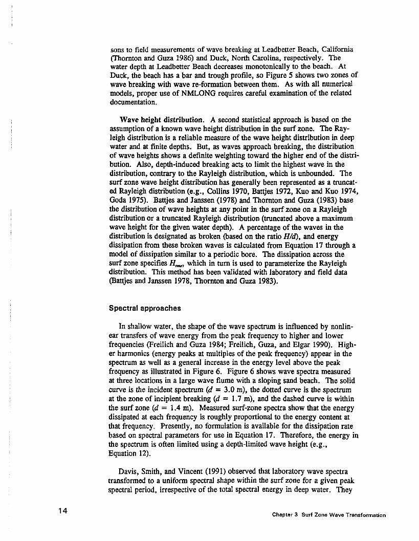
In shallow water, the shape of the wave spectrum is influenced by nonlinear transfers of wave energy from the peak frequency to higher and lower frequencies (Freilich and Guza 1984; Freilich, Guza, and Elgar 1990). Higher harmonics (energy peaks at multiples of the peak frequency) appear in the spectrum as well as a general increase in the energy level above the peak frequency as illustrated in Figure 6. Figure 6 shows wave spectra measured at three locations in a large wave flume with a sloping sand beach. The solid curve is the incident spectrum (d = 3.0 m), the dotted curve is the spectrum at the zone of incipient breaking (d = 1.7 m), and the dashed curve is within the surf zone (d = 1.4 m). Measured surf-zone spectra show that the energy dissipated at each frequency is roughly proportional to the energy content at that frequency. Presently, no formulation is available for the dissipation rate based on spectral parameters for use in Equation 17. Therefore, the energy in the spectrum is often limited using a depth-limited wave height (e.g., Equation 12).

Davis, Smith, and Vincent (1991) observed that laboratory wave spectra transformed to a uniform spectral shape within the surf zone for a given peak spectral period, irrespective of the total spectral energy in deep water. They


~~----------------------------------------~ ~ __ d=3.0m

........... d= 1.7m _____ .d = 1.4 m

.. 'O~----~------r-----~----~------~-----r----~ ~~ ~ ~ ~ u u ~ u

Frequency (Hz)

Figure 6. Shallow-water wave spectra (solid -incident, d = 3.0 m; dot-incipient breaking, d = 1.7 m; dash - surf zone, d = 1.4 m)

parameterized the spectrum in the surf zone based on a modification of the FRF spectrum (named for the Field Research Facility (FRF) of the U.S. Army Engineer Waterways Experiment Station Coastal Engineering Research Center) (Miller and Vincent 1990). The FRF spectrum is expressed as

where

EFRF = spectral energy at frequency f ao = equilibrium range constant (= 0.0029) {JFRF = spectral wave energy parameter k = wave number w f t -y (I

= = = = =

radian wave frequency frequency peak frequency spectral peakedness factor spectral width parameter

(21)

Regression analysis was used to correlate the spectral parameters ({JFRF' -y, (I)

to the incident wave characteristics. In application of the FRF spectrum to


16

prototype conditions, the parameter flERE' is equivalent to the 10-m elevation wind speed. In the laboratory experiments, however, the wave spectra were generated by a wave paddle and not the wind. Under such conditions, flnF is a spectral parameter representing the wave energy, but not related to wind speed. The regression analysis gave the following results for the limiting (maximum) energy levels for the FRF spectrum:

PFRPc

__ 3.24(H.)h 0]°·92 outsUk surf zone (22)

= 3.2 inside surf zone

where C is wave celerity (= Lrr~

and

( h ]0.84

y = 126 -. Lo

(1 = 0.11

(23)

(24)

for 0.008 ~ (H".)./Lo ~ 0.044 and tan fJ = 1130. Equations 23 and 24 have not been tested for a wide range of incident spectral shapes; thus, they should be used with caution. Equations 21 through 24 are applied in the spectral wave propagation model STW A VE (Cialone et ale 1992) to limit wave energy due to breaking.


4 Wave Attenuation Over Reefs

Many tropical coastal regions are fronted by coral reefs. These reefs offer protection to the coast because waves break on the reefs, so the waves reaching the shore are much reduced in height. Reefs typically have steep seaward slopes with broad, flat reef tops and a deeper lagoon shoreward of the reef. The transformation of waves across coral reefs is a complex problem, including the processes of refraction, shoaling, breaking, energy dissipation by bottom friction, and reflection.

Wave Processes

As waves pass from deep water over a steep reef face onto the reef fla~ the waves become highly nonlinear. Wave energy is dissipated due to breaking, but energy is also transferred to both higher and lower frequencies in the wave spectrum, and the spectral shape becomes flat (young 1989, Hardy and Young 1991). The peak wave period shoreward of the reef face may become shorter as higher harmonics are transmitted as free waves (Lee and Black 1978), or the period may increase as surf beat dominates the spectrum. Breaking waves induce a setup of the water surface over the reef, and differences in breaking characteristics along the reef can cause variations in wave setup, producing significant longshore currents. Although it may seem that wave reflection off a nearly vertical reef would be significant, field data (young 1989; Roberts, Murray, and Suhayda 1975) have shown the reflected wave height to be on the order of only 10 percent of the incident height (due to the porosity of the reef). Energy losses due to bottom friction are usually negligible in wave transformation across sandy beach proflles, but may be significant over shallow, rough reef flats where the bottom friction coefficient may be an order of magnitude larger than for a sandy bed (Roberts, Murray, and Suhayda 1975; Gerritsen 1980).

Wave breaking

For engineering purposes, the most significant wave transformation process on a reef is generally depth-limited breaking. Design wave heights for a breaking wave on a structure are often determined from a bottom slope-depen-

Chapter 4 Wave Attenuation Over Reefs 17

18

dent maximum height-to-depth ratio at the toe of the structure (or just offshore). Over a flat reef, this would predict breaking wave heights of 0.78 times the depth. This breaking wave height ratio is overly conservative for design wave heights on the shoreward edge of a wide reef or in the lagoon behind.

The concept of a constant height-to-depth ratio in the surf zone is incorrect; prototype data show the height-to-depth ratio varying between 1.1 and 0.4 across reefs (Gerritsen 1980, Hardy et al. 1990). Similar to the case of waves breaking on a barred beach, waves on a reef flat will break, dissipating energy, and then re-form as they travel across the reef. Wave height will decay quickly on the outer portion of the reef until it reaches a stable value. On the inner portion of the reef, the re-formed wave will decay slowly due to bottom friction. The breaking and re-formation process is strongly dependent on the width of the reef and the water depth over the reef. To accurately estimate wave heights on the reef or in a lagoon, it is necessary to model transformation across the entire reef and to represent wave setup (driven by the gradient in wave height). Wave height estimates based only on incident wave conditions and stiJI-water depths over the reef will not be reliable across the entire reef.

Breaker models

Wave breaking and re-formation on a reef are similar to the process on a barred beach (see Chapter 3). Gerritsen (1980) first applied wave breaking methods developed for mildly sloping beaches to reefs, with the inclusion of dissipation due to bottom friction. Gerritsen applied the random breaking wave model developed by Battjes and Janssen (1978), but found that the truncated Rayleigh distribution of wave heights assumed by Battjes and Janssen was a poor representation of broken waves over a reef. Young (1989) used a similar approach, but included a check to "tum off" wave breaking when the height-to-depth ratio was less than 0.78, to simulate wave re-formation.

The Dally, Dean, and Dalrymple (1985) wave breaking and re-formation model has been extensively verified for plane beaches, composite beach slopes, and barred beach profiles. The model is based on the transformation of individual waves, but may be applied to a random wave field using a statistical approach. The statistical approach requires specification of the wave height distribution in the offshore region, but does not impose a specified distribution in the surf zone. The advantages of the Dally, Dean, and Dalrymple model are: a) extensive verification for a variety of beach configurations, b) no a priori specification of the wave height distribution in the surf zone, and c) the individual wave approach allows calculation of the wave height distribution and statistical wave height parameters (HI7/U' HlIJ, H1I10) in the surf zone. Due to these advantages, the Dally, Dean, and Dalrymple model is recommended to calculate wave attenuation over reefs.

Chapter 4 Wave Attenuation Over Reefs

Modeling Methodology

The methodology described here includes the processes of wave shoaling, refraction, depth-limited breaking, and bottom friction. The assumptions include: linear wave theory, steady-state wave conditions, Rayleigh wave height distribution in the offshore, and longshore homogeneity. The method neglects energy shifts within the wave spectrum, wave-current interaction, and wave reflection and scattering.

The steady-state energy balance equation governing wave propagation is given by

_o_<E---,C,!.-cos_6_} = ~ (E C _ E C , + _p_C_, ( 21tH )3 dx d' "6 1t T sinh (k d)

where

E = wave energy (= p g /fIB for linear wave theory) C,,, = wave group speed associated with the stable wave height p = density of water c;. = bottom friction coefficient

(25)

The first term on the right side of Equation 25 is the energy dissipation due to wave breaking (Dally, Dean, and Dalrymple 1985) (see Equations 17 and 18), and the second term is energy dissipation due to bottom friction (Gerritsen 1980, Thornton and Guza 1983). The application of Equation 25 to calculate random wave transformation across reefs is based on the approach of Larson and Kraus (1991). The input parameters required include the cross-shore profile of the reef and the offshore wave period, mean direction, and rootmean-square height H",.,. The wave-breaking parameters (height -to-depth ratio for incipient breaking lb, Ie, and r) and bottom friction coefficient must also be specified (Gerritsen suggests values of '1 = 0.05 to 0.25 for coral reefs). From the specified offshore Hrrru, a Rayleigh distribution of wave heights is determined. Individual wave heights are randomly chosen from the Rayleigh distribution, and each individual wave is transformed independently. Wave angles are calculated by Snell's law, wave setup is calculated from the crossshore balance of momentum, driven by cross-shore gradients in wave height (Longuet-Higgins and Stewart 1964), and wave height is calculated from Equation 25. The wave height statistic H"", is determined across the reef by combining the transformed individual waves. Other wave height statistics, e.g., H1I3 or HJIlO> may also be calculated. Generally 100 or more individual waves are required for stable mean statistics.

Sample Results

Limited validation of the method described above was performed using laboratory data from a flume study with a configuration replicating the reef at Agat, Guam, and field data from Yonge Reef, Australia (young 1989). The

Chaptar 4 Wava Attenuation Over Reefs 19

20

laboratory study was conducted in an 46-cm-wide flume consisting of 21.3 m of flat bottom, 1.5 m of 115 slope, 10.2 m of 1130 slope, 12.9 m of reef flat, and 3.3 m (covered with wave absorber) of 1130 slope. The water depth in the deepest portion of the flume was 0.69 to 0.64 m with a depth on the reef flat of 0.05 to 0.005 m. Wave periods ranged from 1.1 to 2.5 sec and heights ranged from 0.02 to 0.12 m. Laboratory data are summarized in Appendix A. The model was applied with the standard breaking parameters (K = 0.15 and r = 0.4) and an incipient breaker index "(II = 1.0 (a breaking index of 0.8 is commonly used on gently sloping beaches, but an index of 1.0 is more appropriate for steeper seaward reef slopes). The bottom friction coefficient was set to 0.01, which is a typical value for smooth slopes such as the lab configuration. Figures 7 through 9 show selected results for the laboratory data. The agreement between laboratory measurements and model results is excellent. The solid line is the modeled wave height, the symbols are the measured wave height, the chain-dot line is the modeled setup, and the dotted line is the still-water level. These results are typical for water depths greater than 3 cm on the reef flat. For shallow water depths, the model underpredicted the (small) measured wave heights. For very shallow depths, wave energy at the incident frequency is almost entirely dissipated and lowfrequency energy (which is not included in the model) dominates. Figure 10 is a scatter plot of the calculated versus measured results for 69 laboratory tests (345 data points). The figure shows the good correlation for the higher wave heights (depths greater than 3 cm) and the underprediction of the low wave heights (depths less than 3 cm).

Figure 11 shows results from a field experiment conducted on Yonge Reef, which is part of the Great Barrier Reef in Australia. This is one of four cases reported by Young (1989). The incident Hrwu = 2.05 m and the depth over the reef was 1.05 m. The wave measurement was taken in the lagoon on the leeward side of the reef. The wave breaking parameters used in the model were identical to those applied for the laboratory cases, and the bottom friction coefficient was 0.05, which is equivalent to the value suggested by Young. As in the case of the laboratory results, the model compares well with the measurements.

Recommendations

For engineering purposes, the breaking wave model of Dally, Dean, and Dalrymple can be used to calculate the attenuation of waves over reefs. For very small water depths over the reef, the model may underpredict wave height as nonlinear processes dominate. The inclusion of bottom friction in the energy balance equation improves estimates of wave height across the reef flat, but may not be critical for engineering·application. There are insufficient measurements to give general guidance of bottom friction coefficients, so sitespecific field measurements are recommended to determine Cf'


$2 test = 18 d

'--_._. __ .-..,. ~-t----------.\. .. =="--------o

~ 9;----r---.----,-----r----.---~---.----.

o 5 10 15 20 25 30


Figure 7. Laboratory test 18, Agat, Guam

a test = 23

IX) o

35

d x

'-'-'-'-'"\ o ~ ._ .. __ .. _._----_ ... _ ... __ .... _ ... _._-_ .. _ .. __ .... \...:="=,-'--------

N, o

40

9~----.---.----,----r---.----~--.----· o 5 10 15 20 25 30 35 40




22

$2 test = 37 d

IX) o d

o ~ ... _-_._ .... _:::::.:===::::::::::::-.=._,-----

N o d~----,-----~----r---~~--~-----r----~----, I

o 5 10 15 20 25 30



~ o d

o o

a

35

d~--~~~---,------------~-----------, 0.00 0.01 0.02 0.03

Measured Hrms (m)

Figure 10. Calculated versus measured laboratory results

40


C! O~--~--~---T--~--~--~~--~~~ __ ~~·

o 200 400 600 800 1000 1200 1400 1600 1800 2000


Agure 11. Field test, August 1985, Yonge Reef, Australia (Young 1989)


24

5 Shoaling and Decay of Multiple Wave Trains

Little information is available on the refraction, shoaling, and breaking of multiple-wave-train systems. Observations in relatively shallow water (4-8 m) indicate that approximately 65 percent of wave fields are comprised of two or more distinct wave trains well separated in the frequency domain (Thompson 1980). Thompson's statistics were from representative sites on the Atlantic, Pacific, and Gulf of Mexico coasts of the United States, and may be indicative of open ocean and coastal conditions worldwide.

Several approaches have been used to estimate the transformation of multiple-peaked wave systems. The traditional, pervasive approach is to assign all wave energy to the dominant peak, then refract and shoal this representative wave, applying a breaking criterion where needed (Larson, Kraus, and Byrnes 1989). Another method is to divide the wave field into two (or more) wave trains and treat each one separately (independent and noninteracting), with a breaking criterion applied to each wave train independently and the results superimposed (Gravens, Scheffner, and Hubertz 1989) or to consider only the most significant peak and disregard other peaks (Kraus et al. 1988). Some existing spectral wave models compute each frequency and direction band of the spectrum independently (O'Reilly and Guza 1991, Resio 1988). Breaking may be treated with a limiting spectral form, an energy sink term in the energy balance equation, or a simple renormalization of the spectrum to match an equivalent monochromatic wave of depth-limited height.

Laboratory Experiments

Laboratory tests were conducted to examine the shoaling and decay of multiple wave trains in a wave flume (Smith and Vincent 1992) and a wave basin (Briggs, Smith, and Green 1991). Double-peaked spectra were determined by superimposing two spectra of the TMA form (Bouws et al. 1985). Two wave period combinations were used, ~ = 2.5/1.25 sec and ~ = 2.5/1.75 sec, with two total zero-moment wave heights, H_ = 15.2 cm and 9.2 cm. The relative splits of energy between the low-frequency and highfrequency peaks were 113:2/3, 112:112, and 2/3:113. In the basin tests, directional spreading of 0 deg, 20 deg, and 40 deg and mean wave directions

Chapter 5 Shoaling and Decay of Multiple Wave Trains

of 0 deg and 20 deg were included in the test series. Both the flume and basin experiments had similar bottom configurations, with a flat concrete bottom near the generators and a 1130 concrete slope. Wave gauges were placed across the slopes to measure the wave transformation with water depth. In the wave basin, two longshore arrays (one on the flat and one on the slope) were also deployed to measure wave direction.

Wave Spectra

Figures 12 through 15 summarize the spectral transformation for four of the cases simulated in the laboratory flume. Figures 12 and l3 present cases corresponding to dual wave trains with peak periods of 2.5 sec and 1.25 sec with H_ = 15.2 cm. Similarly, Figures 14 and 15 present cases with dual wave trains with peak periods of 2.5 sec and 1.75 sec and H_ = 9.2 cm. In Figures 13 and 15 approximately two-thirds of the energy is initially in the low frequency peak, and in Figures 12 and 14 approximately one-third of the energy is initially in the low frequency peak. In each figure, only four of the measured spectra are overlaid - the deepest measurement (h = 61 cm), the shallowest measurement (h = 6.1 cm), and two intermediate-depth measurements (h = 18.3 cm and 9.1 cm) - but these are sufficient to illustrate the basic trends seen in the complete set of data.

b .....

LaJ

i

s;;! 0.0 O.B to t2 t4 t6 tB 0.4 0.6 0.2 2.0

f (Hz)

Figure 12. Energy spectra for Tp = 2.5/1.25 sec, Hmo = 15.2 em (h = 61 em (solid), 18.3 em (dash), 9.1 em (dot), 6.1 em (chain-dot))

Chapter 5 Shoaling and Decay of Multiple Wave Trains 25

26

i

52 0.0 0.2 0.8 1.0 1.2 1.6 1.8 0.4 0.6 2.0

f (Hz)

Figure 13. Energy spectra for Tp = 2.5/1.25 sec, Hmo = 15.2 cm (h = 61 em (solid), 18.3 cm (dash), 9.1 cm (dot), 6.1 cm (chain-dot))

111 "r"

~'iJt 1\\ I.,: \A II \! ; \

I ~I ,j""'\ .v f,.p' \.,~. / 0\. 0 ....... o 0 •

: " : 0

.. " o . ' ! " ....... ~

... IO~--~----~---r--~----~---r--~~--~--~--~ -u ~ U M U W 1.2 U ~ ~ w

f (Hz)

Figure 14. Energy spectra for Tp = 2.5/1.75 sec, Hmo = 9.2 em (h = 61 em (solid), 18.3 em (dash), 9.1 em (dot), 6.1 em (chain-dot))


.. 10 +--..,...---,..-......., __ ,...._..,..-_.....-_....,...._~_.......,~--I -M ~ ~ ~ M W U U ~ ~ w

f (Hz)

Figure 15. Energy spectra for Tp = 2.5/1.75 sec, Hmo = 9.2 cm (h = 61 em (solid), 18.3 em (dash), 9.1 em (dot), 6.1 em (chain-dot))

The trend in the spectral transformation is very similar for each case. Between the depths of 61.0 cm and 18.3 cm, there is a general increase in energy at frequencies both above and below the primary peaks. Also, distinct energy peaks appear at harmonic frequencies due to nonlinear, near-resonance triad interaction (Freilich and Guza 1984). For example, in Figure 12 a secondary peak appears at 1.2 Hz, which is the sum frequency of the two primary peaks at 0.4 Hz and 0.8 Hz. In Figure 15, secondary peaks appear at 0.8 Hz (self-interaction of O.4-Hz peak), 0.97 Hz (interaction of O.4-Hz and 0.57-Hz peaks), and 1.14 Hz (self-interaction of O.4-Hz peak). These examples do not show energy transfer into the valley between the primary peaks as shown by Elgar and Guza (1985), probably because harmonics of the primary peaks do not exist in this Valley. For Figures 12 and 13, the second peak (at 0.8 Hz) was at a harmonic of the first peak (at 0.4 Hz), but this did not seem to affect the spectral transformation since Figures 14 and 15 show the same trends.

Between depths of 18.3 cm and 6.1 cm, wave breaking occurred. Wave breaking lowered the general energy level from the low-frequency peak through all the higher frequencies and, by the shallowest gauge, eliminated all energy peaks above the low-frequency peak. The low-frequency peak became the dominant peak of the spectrum as the waves shoaled and broke. In all test cases, only the low-frequency peak is clearly dominant in the shallowest measurement. This trend was evident whether the peaks were closely placed, the low-frequency peak was initially the lower-energy peak in the spectrum, the


28

total significant wave height was high or low, directional spreading was applied, or the peaks had the same or different mean directions.

Observations show that the dominance of the low-frequency peak is due primarily to the loss of energy in the high-frequency peak. Simulation of each peak in the spectrum individually showed that the low-frequency peak transformed almost identically with and without the high-frequency peak present. The energy at the high-frequency peak decays at deeper depths when the lowfrequency peak is present. Some of this dissipation takes place at depths outside what is traditionally the surf zone.

The reason for the interaction between the two peaks is not understood. One possibility is that resonant interaction among waves transfers energy out of the higher-frequency peak to even higher frequencies, where it is rapidly dissipated. Another possibility is that the bottom friction for the two-peak case may be substantially different. However, it is not clear why all the loss should be at the high frequencies. A third possibility is a shoaling analog of the mechanism proposed by Banner and Phillips (1974) in which the highfrequency waves see the underlying low-frequency waves in terms of a largescale flow that enhances breaking of the shorter waves with no apparent effect on the longer waves. Which, if any, of these explanations is correct remains to be seen.

Wave Heights

Figures 16 and 17 show the transformation of HJ13 and H_, respectively, as a function of the mean water depth for the cases with dual peaks of 2.5 sec and 1.25 sec. The upper three curves on each plot are the high-energy cases (total initial wave height of 15.2 cm) with three different distributions of energy between the two peaks (as labeled on the plot). The lower three curves are the low-energy cases (total initial wave height of 9.2 cm) with the same three distributions of energy between the two peaks. HJ13 tends to increase as the water depth decreased due to shoaling, then decreases quickly when the depth is approximately twice the height. H_ tends to stay approximately constant until a depth of about twice the wave height, then H_ decreases quickly. The most striking feature in these plots is the difference in HJ13 due to the different distributions of energy between the high- and lowfrequency peaks (Figure 16). The maximum difference in HJ13 is 23 percent between the case with two-thirds of the energy in the low-frequency peak and the case with one-third of the energy in the low-frequency peak. The maximum difference occurs in the region of the maximum wave height. For the dual peaks of 2.5 sec and 1.75 sec, the different distributions of energy had a smaller effect. The maximum difference in HJ13 is 8 percent. H_ is less influenced by the distribution of energy between the peaks. The maximum difference in H_ is 13 percent for dual peaks of 2.5/1.25 sec and 6 percent for dual peaks of 2.5/1.75 sec.


~

0 ;i.

0 ~

~ ~

J~ s

:::c ~

0

"" 0 N

~ 0.0 10.0

~"""-'--, ~ ........ -----

;,:/....... . ...................................... :.=--

it _____ : "--'" ... ............. ... . ............ ~::-------- ..

............... ::::::: .. : .. ::::::: .:.--:--- -

20.0

T p (sec) = 2.50/t25 Energy Distribution __ low freq V3 - hig, freq 2/3 _ .......... Iow freq V2 - hig, freq V2 __ .Iow freq 2/3 - hig, freq V3

30.0 <40.0 SO.O 60.0

Depth (ern)

Figure 16. H,/3 versus mean water depth (Tp = 2.5/1.25 sec)

70.0

~~------------------------------------------,

o

",-----------y.: ................. _-_ .................................... ,.

1// l

) ?:.:.---.' 0' .......... ::::::.:.:::::::.:::::::::.:.==::.-.. -

'"

T p (sec) = 2.50/t25 Energy Distribution __ low freq V3 - hig, freq 2/3 ... _ ... __ .. Iow freq V2 - hig, freq V2 __ .Iow freq 2/3 - hig, freq V3

d4-----~----~----~----~----~~----~--~ 0.0 10.0 20.0 30.0 <40.0 SO.O 60.0 70.0

Depth (em)

Figure 17. Hmo versus mean water depth (Tp = 2.5/1.25 sec)


30

Thus, the distribution of energy between two peaks can have a significant impact on the nearshore wave height transformation. The impact is greater on H1I3 than Hmo. The proximity of the peaks also affects transformations. Relatively close peaks are less affected by different distributions of energy than more separated peaks.

Summary

Laboratory simulation of two wave trains shoaling and breaking on a plane beach indicates that there are strong interactions between the wave trains. Simple approaches to estimating the transformation of multiple wave trains, such as treating the wave trains independently (and superimposing the results) or neglecting one of the wave trains can lead to significant errors in estimating wave height and period in the surf zone.

The significant wave height defined from an analysis of individual waves differed by more than 20 percent from case to case depending on the locations and relative sizes of the two peaks and overall energy level. This is of engineering significance and indicates that information on the spectral content of the wave field is needed to make accurate predictions. The spectrally based significant wave height varied by about 10 percent depending on location and relative size of the two peaks, which may not be of engineering significance.

Analysis of the wave spectra indicates that the low-frequency peak becomes dominant, especially in shallower water. This results from the preferential loss of energy in the high-frequency peak. Consequently, methods that ignore the lower frequency peak or superimpose results may underestimate the wave period in shallow water. Mean direction and directional spreading had little influence on the laboratory results for these plane-beach experiments.


6 Conclusions

This report summarizes the nearshore wave breaking and decay research performed under the Nearshore Waves and Currents work unit. The work has emphasized wave decay through the surf zone, which is required to estimate nearshore hydrodynamics (longshore and cross-shore currents and wave setup), flooding and storm damage, and nearshore sediment transport. Incipient breaker indices, surf zone wave decay expressions, spectral shapes in the surf zone, wave breaking on reefs, and decay of mUltiple wave trains are included in the report.

Areas for future research include:

a. Wind effects on wave breaking and decay. Existing studies on wind effects have been qualitative and have not provided quantitative relationships.

b. Roughness effects on wave decay over reefs. Field measurements of wave decay across rough coral reefs at a variety of locations are required to quantify wave decay due to bottom friction.

C. Current influence on wave breaking. The impact of strong longshore currents, undertow, and ebb/flood currents (e.g., at an inlet) on depthlimited wave breaking has not been evaluated.

d. Detailed modeling of the energy dissipation in breaking waves. To extend wave decay modeling beyond empirical methods, the details of wave breaking, including generation and dissipation of turbulence, must be included.

e. Incorporation of infragravity waves into wave breaking and decay models. Surf beat and edge waves slowly vary the mean water level and the mean flow, but the effect of these long waves has not been included in wave decay modeling.

f Extending nonlinear wave models (e.g., Freilich and Guza 1984) to the surf zone with continued research on the interaction on multiple wave trains in the surf zone.

Chapter 6 Conclusions 31

32

References

Banner, M. L., and Phillips, O. M. (1974). "On small scale breaking waves," Journal of Fluid Mechanics 65, 647-657.

Battjes, J. A. (1972). "Set-up due to irregular waves." 1hineenth Coastal Engineering Conference. American Society of Civil Engineers, 1993-2004.

_~ __ . (1974). "Surf similarity." Fourteenth Coastal Engineering Conference. American Society of Civil Engineers, 466-480.

Battjes, J. A., and Janssen, J. P. F. M. (1978). "Energy loss and setup due to breaking of random waves." Sixteenth Coastal Engineering Conference. American Society of Civil Engineers, 569-587.

Bouws, E., Gunther, H., Rosenthal, W., and Vincent, C. L. (1985). "Similarity of the wind wave spectrum in finite depth water; 1. spectral form, " Journal of Geophysical Research 90(Cl), 975-986.

Bowen, A. J. (1969). "The generation of longshore currents on a plane beach," Journal of Marine Research 27(1), 206-215.

Briggs, M. J., Smith, J. M., and Green, D. R. (1991). "Wave transformation over a generalized beach," Technical Report CERC-9I-5, U.S. Army Engineer Waterways Experiment Station, Vicksburg, MS.

Camfield, F. E. (1991). "Wave forces on wall," Journal of Waterway, Port, Coastal, and Ocean Engineering 117(1), 76-79.

Cialone, M. A., Mark, D. J., Chou, L. W., Leenknecht, D. A., Davis, J. E., Lillycrop. L. S., and Jensen, R. E. (1992). "Coastal Modeling System (CMS) user's manual," Instruction Report CERC-9I-I, Supplement 1, U.S. Army Engineer Waterways Experiment Station, Vicksburg, MS.

Collins, J. I. (1970). "Probabilities of breaking wave characteristics." Twelfth Coastal Engineering Conference. American Society of Civil Engineers, 1993-2004.

References

Dally, W. R. (1990). "Random breaking waves: A closed-form solution for planar beaches," Coastal Engineering 14(3), 233-263.

____ . (1992). "Random breaking waves: Field verification of a wave-by-wave algorithm for engineering application," Coastal Engineering 16, 369-397.

Dally, W. R., Dean, R. G., and Dalrymple, R. A. (1985). "Wave height variation across beaches of arbitrary profile," Journal oj Geophysical Research 90(C6), 11917-11927.

Davis, J. E., Smith, J. M., and Vincent, C. L. (1991). "Parametric description for a wave energy spectrum in the surf zone," Miscellaneous Paper CERC-91-11, U.S. Army Engineer Waterways Experiment Station, Vicksburg, MS.

Divoky, D., LeMehaute, B., and Lin, A. (1970). "Breaking waves on gentle slopes," Journal of Geophysical Research 75(9), 1681-1692.

Douglass, S. L. (1990). "Influence of wind on breaking waves," Journal oj Waterway, Pon, Coastal, and Ocean Engineering 116(6), 651-663.

Ebersole, B. A. (1987). "Measurement and prediction of wave height decay in the surf zone. " Coastal Hydrodynamics. American Society of Civil Engineers, 1-16.

Elgar, S., and Guza, R. T. (1985). "Shoaling gravity waves: comparisons between field observations, linear theory, and a nonlinear model," Journal of Fluid Mechanics 158,47-70.

Freilich, M. R., and Guza, R. T. (1984). "Nonlinear effects on shoaling surface gravity waves." Philosophical Transactions. Royal Society of London, A311, 1-41.

Freilich, M. R., Guza, R. T., and Elgar, S. L. (1990). "Observations of nonlinear effects in directional spectra of shoaling gravity waves," Journal of Geophysical Research 95(C6), 9645-9656.

Galloway, J. S., Collins, M. B., and Moran, A. D. (1989). "Onshore/offshore wind influence on breaking waves: an empirical study," Coastal Engineering 13, 305-323.

Galvin, C. J. (1968). "Breaker type classification on three laboratory beaches," Journal of Geophysical Research 73(12),3651-3659.

----. (1969). "Breaker travel and choice of design wave height," Journal oj the Waterways and Harbors Division 95(WW2), 175-200.

References 33

34

Gerritsen, F. (1980). "Wave attenuation and wave set-up on a coastal reef." Seventeenth Coastal Engineering Conference. American Society of Civil Engineers, 444-461.

Goda, Y. (1970). "A synthesis of breaker indices," Transactions of the Japan Society of avil Engineers 2(2),227-230.

____ . (1975). "Irregular wave deformation in the surf zone," Coastal Engineering in Japan 18, 13-26.

Gravens, M. B., Scheffner, N. W., and Hubertz, J. M. (1989). "Coastal processes from Asbury Park to Manasquan, New Jersey," Miscellaneous Paper CERC-89-11, U.S. Army Engineer Waterways Experiment Station, Vicksburg, MS.

Hardy, T. A., and Young, I. R. (1991). "Modelling spectral wave transformation on a coral reef flat." Australasian Conference on Coastal and Ocean Engineering, 345-350.

Hardy, T. A., Young, I. R., Nelson, R. C., and Gourlay, M. R. (1990). "Wave attenuation of an offshore coral reef." 1Wenry-second Coastal Engineering Conference. American Society of Civil Engineers, 330-334.

Horikawa, K., and Kuo. C. (1966). "A study on wave transformation inside the surf zone." Tenth Coastal Engineering Conference. American Society of Civil Engineers, 235-249.

Hwang, L., and Divoky, D. (1970). "Breaking wave setup and decay on gentle slope." Twelfth Coastal Engineering Conference. American Society of Civil Engineers, 377-389.

Iversen, H. W. (1952). "Waves and breakers in shoaling water." Third Coastal Engineering Conference. American Society of Civil Engineers, 1-12.

Iwagaki, Y., Sakai, T. Tsukioka, K., and Sawai, N. (1974). "Relationship between vertical distribution of water particle velocity and type of breakers on beaches," Coastal Engineering in Japan 17, 51-58.

Komar, P. D., and Gaughan, M. K. (1972). "Airy wave theory and breaker height prediction." Thirteenth Coastal Engineering Conference. American Society of Civil Engineers, 405-418.

Kraus, N. C., and Larson, M. (1991). "NMLONG: Numerical model for simulating the longshore current; Report 1: Model development and tests," Technical Report DRP-91-1, U.S. Army Engineer Waterways Experiment Station, Vicksburg, MS.

Kraus, N. C., Scheffner, N. W., Hanson, H., Chou, L. W., Cialone, M. A., Smith, J. M., and Hardy, T. A. (1988). "Coastal processes at Sea Bright

References

to Ocean Township, New Jersey," Miscellaneous Paper CERC-88-12, U.S. Army Engineer Waterways Experiment Station, Vicksburg, MS.

Kuo, C. T., and Kuo, S. T. (1974). "Effect of wave breaking on statistical distribution of wave heights." Civil Engineering Oceans, 1211-1231.

Larson, M., and Kraus, N. C. (1991). "Numerical model of longshore current for bar and trough beaches," Journal oJ Waterway, Port, Coastal, and Ocean Engineering 117(4), 326-347.

Larson, M., Kraus, N. C., and Byrnes, M. R. (1989). "SBEACH: Numerical model for simulating storm-induced beach change; Report 2, Numerical formulation and model tests," Technical Report CERC-89-9, U.S. Army Engineer Waterways Experiment Station, Vicksburg, MS.

Lee, T. T., and Black, K. P. (1978). "The energy spectra of surf waves on a coral reef." Sixteenth Coastal Engineering Conference. American Society of Civil Engineers, 588-608.

LeMQlaut~, B. (1962). "On the nonsaturated breaker theory and the wave run up." Eighth Coastal Engineering Conference. American Society of Civil Engineers, 77-92.

Longuet-Higgins, M. S. (1970a). "Longshore currents generated by obliquely incident sea waves, 1," Journal oj Geophysical Research 75(33), 6778-6789.

_____ . (1970b). "Longshore currents generated by obliquely incident sea waves, 2," Journal oj Geophysical Research 75(33), 6790-6801.

Longuet-Higgins, M. S., and Stewart, R. W. (1963). "A note on wave setup," Journal oj Marine Research 21(1),4-10.

_____ . (1964). "Radiation stresses in water waves; a physical discussion, with applications," Deep-Sea Research II, 529-562.

Maruyama, K., Sakakiyama, T., Kajima, R., Saito, S., and Shimizu, T. (1983). "Experimental study on wave height and water particle velocity near the surf zone using a large wave flume," Civil Engineering Laboratory Report No. 382034, The Central Research Institute of Electric Power Industry, Chiba, Japan (in Japanese).

McCowan, J. (1891). "On the solitary wave, n Philosophical Magazine 36, 5th Series, 430-437.

Miller, H. C., and Vincent, C. L. (1990). "FRF spectrum: TMA with Kitaigorodskii's f4 scaling," Journal oJ Waterway, Port, Coastal, and Ocean Engineering 116(1),57-78.

References 35

36

Mizuguchi, M. (1980). "An heuristic model L.f wave height distribution in surf zone." Seventeenth Coastal Engineering Conference. American Society of Civil Engineers, 278-289.

Munk, W. H. (1949). "The solitary wave theory and its applications to surf problems," Annals of the New York Academy of Sciences 51, 376-462.

O'Reilly, W. C., and Guza, R. T. (1991). "Comparison of spectral refraction and refraction-diffraction wave models," Journal of Waterway, Pon, Coastal, and Ocean Engineering 117(3),199-215.

Resio, D. T. (1988). "A steady-state wave model for coastal application." 1Wenty-.first Coastal Engineering Dmference. American Society of Civil Engineers, 929-940.

Roberts, H. H., Murray, S. P., and Suhayda, J. N. (1975). "Physical processes in a fringing reef system," Journal of Marine Research 33, 233-260.

Saeki, H., and Sasaki, M. (1973). II A study of the deformation of waves after breaking (1)." 1Wentieth Japanese Conference on Coastal Engineering. Japan Society of Civil Engineers, 559-564 (in Japanese).

Singamsetti, S. R., and Wind, H. G. (1980). "Characteristics of breaking and shoaling periodic waves normally incident on to plane beaches of constant slope," Report M1371, Delft Hydraulic Laboratory, Delft, The Netherlands.

Smith, E. R., and Kraus, N. C. (1991). "Laboratory study of wave-breaking over bars and artificial reefs," Journal of Waterway, Pon, Coastal, and Ocean Engineering 117(4), 307-325.

Smith, J. M., and Kraus, N. C. (1988). "An analytical model of wave-induced longshore current based on power law wave height decay," Miscellaneous Paper CERC-88-3, U.S. Army Engineer Waterways Experiment Station, Vicksburg, MS.

Smith, J. M., and Vincent, C. L. (1992). "Shoaling and decay of two wave trains on beach," Journal of Waterway, Pon, Coastal, and Ocean Engineering 118(5),517-533.

Stive, M. J. F. (1985). "A scale comparison of waves breaking on a beach," Coastal Engineering 9(2), 151-158.

Sunamura, T. (1980). "A laboratory study of offshore transport of sediment and a model for eroding beaches." Seventeenth Coastal Engineering Conference. American Society of Civil Engineers, 1051-1070.

Svendsen, I. A. (1984). "Wave heights and setup in a surf zone," Coastal Engineering 8(4), 303-329.

References

Svendsen, I. A., Madsen, P. A., and Hansen, J. B. (1978). "Wave characteristics in the surf zone." Sixteenth Coastal Engineering Conference. American Society of Civil Engineers, 520-539.

Thompson, E. F. (1980). Energy spectra in shallow U.S. coastal waters," Technical Paper No. 80-2, Coastal Engineering Research Center, U.S. Army Corps of Engineers, Fort Belvoir , VA.

Thornton, E. B. (1970). "Variation of longshore current across the surf zone." Twelfth Coastal Engineering Conference. American Society of Civil Engineers, 291-308.

Thornton, E. B., and Guza, R. T. (1983). "Transformation of wave height distribution," Journal of Geophysical Research 88(CI0), 5925-5938.

_~:-:--:---' (1986). "Surf zone longshore currents and random waves: field data and models," Journal of Physical Oceanography 16, 1165-1178.

Visser, P. J. (1982). "The proper longshore current in a wave basin," Report No. 82-1, Laboratory of Fluid Mechanics, Department of Civil Engineering, Delft University of Technology, Delft, The Netherlands.

Walker, J. R. (1974). "Wave transformations over a sloping bottom and over a three-dimensional shoal," Miscellaneous Report No. II, University of Hawaii, Look Lab-75-11, Honolulu, HI.

Weggel, J. R. (1972). "Maximum breaker height," Journal of the Waterways, Harbors and Coastal Engineering Division 98(WW4), 529-548.

Young, I. R. (1989). "Wave transformation over coral reefs," Journal of Geophysical Research 94(C7), 9779-9789.

References 37

Appendix A Agat Laboratory Wave Measurements

A laboratory study of wave decay across the reef at Agat, Guam, was conducted in a 46-cm-wide flume. Starting at the shoreward end, the flume consisted of 3.3 m (covered with wave absorber) of 1130 slope, 12.9 m of reef flat (0 slope), 10.2 m of 1130 slope, 1.5 m of 115 slope, and 21.3 m of flat bottom. The waves were measured at six locations across the profile at distances of 38.0 m (Gauge 1), 13.78 m (Gauge 2), 12.04 m (Gauge 3), 9.66 m (Gauge 4), 8.48 m (Gauge 5), and 6.25 m (Gauge 6) from the shoreward end of the flume. Table A 1 gives the zero-moment wave height Hmo, peak wave period Tp , maximum wave height Hmax, and the mean water level 1/ (relative to the still-water level) for 69 test cases. The still-water depth h in the deepest portion of the flume is also given in Table A 1. Plots of the laboratory measurements and wave model predictions for three of the test cases are given in Figures 7-9 in the main text.

Appendix A Agat Laboratory Wave Measurements A1

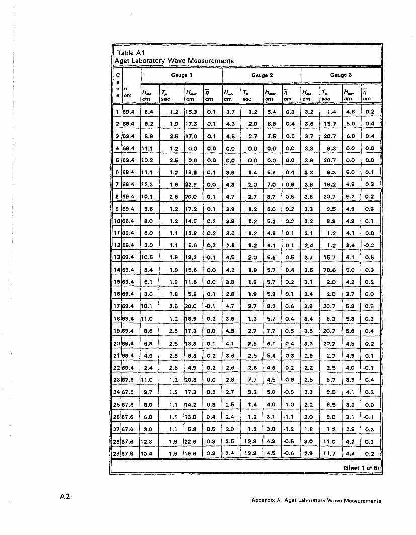
Table A1 Agat laboratory Wave Measurements

c Gauge 1 Gauge 2 Gauge 3

" s h H_ T" H_. - H_ T,. H_. - H_ T,. H_ -e em II fI fI

em sec em em em tlec em em cm sec em em

1 69.4 8.4 1.2 15.3 0.1 3.7 1.2 5.4 0.3 3.2 1.4 4.8 0.2

2. 69.4 9.2 1.9 17.3 0.1 4.3 2.0 5.9 0.4 3.6 15.7 5.0 0.4

3 69.4 8.9 2.5 17.6 0.1 4.5 2.7 7.5 0.5 3.7 20.7 6.0 0.4

4 69.4 11.1 1.2 0.0 0.0 0.0 0.0 0.0 0.0 3.3 9.3 0.0 0.0

5 69.4 10.2 2.5 0.0 0.0 0.0 0.0 0.0 I 0.0 3.9 20.7 0.0 0.0

6 69.4 , 1.1 1.2 18.9 0.1 3.9 1.4 5.9 0.4 3.3 9.3 5.0 0.1

7 69.4 12.3 1.9 22.9 0.0 4.8 2.0 7.0 0.6 3.9 16.2 6.9 0.3

8 69.4 10.1 2.5 20.0 0.1 4.7 2.7 8.7 0.6 3.8 20.7 5.2 0.2

9 89.4 9.6 1.2 17.2 0.1 3.9 1.2 6.0 0.2 3.3 9.5 4.9 0.3

10 69.4 8.0 1.2 14.5 0.2 3.B 1.2 5.2 0.2 3.2 8.9 4.9 0.1

11 69.4 6.0 1.1 12.8 0.2 3.6 1.2 4.9 0.1 3.1 1.2 4.1 0.0

12 69.4 3.0 1.1 6.6 0.3 2.6 1.2 4.1 O. , 2.4 1.2 3.4 .0.2

13 69.4 10.5 1.9 19.3 .0.1 4.5 2.0 5.6 0.5 3.7 15.7 6.1 0.5

14 69.4 8.4 1.9 15.6 0.0 4.2 1.9 6.7 0.4 3.5 78.6 5.0 0.3

15 69.4 6.1 1.9 11.6 0.0 3.8 1.9 5.7 0.2 3.1 2.0 4.2 0.2

16 169.4 3.0 1.8 5.8 0.1 2.8 1.9 5.8 0.1 2.4 2.0 3.7 0.0

17 69.4 10.1 2.5 20.0 -C.l 4.7 2.7 8.2 0.6 3.9 20.7 6.8 0.5

18 69.4 11.0 1.2 18.9 0.2 3.9 1.3 5.7 0.4 3.4 9.3 5.3 0.3

19 69.4 8.6 2.5 17.3 0.0 4.5 2.7 7.7 0.5 3.6 20.7 5.6 0.4

20 69.4 6.8 2.5 13.8 0.1 4.1 2.5 6.1 0.4 3.3 20.7 4.5 0.2

21 69.4 4.9 2.5 9.8 0.2 3.6 2.5 5.4 0.3 2.9 2.7 4.9 0.1

22 69.4 2.4 2.5 4.9 0.2 2.6 2.5 4.6 0.2 2.2 2.5 4.0 -C.l

23 67.6 11.0 1.2 20.8 0.0 2.8 7.7 4.5 .0.9 2.5 9.7 3.9 0.4

24 67.6 9.7 1.2 17.3 0.2 2.7 9.2 5.0 ·0.9 2.3 9.5 4.1 0.3

25 67.6 8.0 1.1 14.2 0.3 2.5 1.4 4.0 -1.0 2.2 9.5 3.3 0.0

r~ 0.4 2.4 1.2 3.1 -1.1 2.0 .

67.6 6.0 1.1 13.0 9.0 3.1 -C.l

27 67.6 3.0 1.1 5.8 0.5 2.0 1.2 3.0 -1.2 1.8 1.2 2.8 -C.3

28 67,6 12.3 1.9 122.6 0.3 3.5 12.8 4.9 -C.5 3.0 11.0 4.2 0.3

29 67.6 10.4 1.9 i'9•6 0.3 3.4 12.S 4.5 .0.6 2.9 11.7 4.4 0.2

A2 Appendix A Agat Laboratory Wave Measurements

I~A1 (Continued)

C Gauge 4 Gauge 5 Gauge 6 a s h H_ T,. - T,. - H_ T,. H_K -

em H_ f} H_ H_ f} f}

e em sec em em em sec em em em sec em em

1 69.4 2.8 1.4 3.8 0.2 2.7 9.3 4.4 0.2 2.6 1.3 3.8 0.2

2 69.4 3.1 78.6 4.6 0.4 3.0 78.6 4.5 0.4 2.9 78.6 4.5 0.4

3 69.4 3.1 13.3 5.3 0.5 3.0 9.2 5.5 0.5 2.9 80.0 4.5 0.5

4 69.4 2.9 9.5 0.0 0.0 2.8 9.5 0.0 0.0 2.7 70.0 0.0 0.0

5 69.4 3.3 13.3 0.0 0.0 3.2 80.0 0.0 0.0 3.1 46.7 0.0 0.0

6 69.4 3.0 9.5 5.4 0.5 2.9 9.5 4.4 0.3 2.7 70.0 4.5 0.5

7 69.4 3.5 78.6 6.0 0.7 3.3 78.6 5.3 0.5 3.2 50.0 5.2 0.8

8 69.4 3.3 13.7 6.0 0.7 3.2 80.0 5.9 0.5 3.1 46.7 4.4 0.8

9 69.4 2.9 1.1 4.1 0.3 2.7 9.5 4.1 0.2 2.6 70.0 4.0 0.3

10 69.4 2.8 1.4 4.1 0.2 2.7 1.4 4.4 0.2 2.6 1.4 4.1 0.2

11 69.4 2.7 1.4 4.0 0.1 2.6 1.4 3.7 0.1 2.5 1.4 3.5 0.1

12 69.4 2.2 1.2 3.1 -a.l 2.1 1.2 3.1 -a.l 2.1 1.4 3.0 -0.1

13 69.4 3.3 78.6 5.2 0.5 3.2 78.6 4.8 0.5 3.0 78.6 4.8 0.6

14 69.4 3.0 78.6 4.9 0.4 3.0 78.6 5.2 0.4 2.9 78.6 3.9 0.5

15 69.4 2.8 78.6 4.4 0.2 2.7 78.6 4.8 0.2 2.6 78.6 4.1 0.3

16 69.4 2.3 1.0 3.4 0.0 2.2 1.9 3.2 0.0 2.2 1.9 3.3 0.1

17 69.4 3.3 13.7 5.6 0.6 3.2 80.0 5.8 0.6 3.1 80.0 4.7 0.7

18 69.4 3.0 9.5 5.0 0.3 2.8 9.5 4.5 0.3 2.7 70.0 4.6 0.3

19 69.4 3.1 13.3 4.7 0.4 3.0 9.2 4.5 0.5 2.9 80.0 4.6 0.5

20 69.4 2.9 13.3 4.7 0.3 2.8 9.0 4.5 0.3 2.7 20.7 4.5 0.4

21 69.4 2.6 13.0 4.0 0.1 2.6 0.9 4.5 0.2 2.5 20.7 4.0 0.2

22 69.4 2.0 1.4 3.2 0.0 2.0 1.4 2.8 0.0 1.9 1.4 3.8 0.1

23 67.6 2.0 9.5 3.1 0.5 1.9 9.7 3.7 0.5 1.7 70.0 2.9 -1.0

24 67.6 1.9 9.2 3.0 0.4 1.8 9.5 3.3 0.4 1.7 70.0 3.2 -1.0

25 67.6 1.8 9.0 3.4 0.3 1.7 9.5 3.0 0.3 1.6 70.0 2.4 -1.0

26 67.6 1.7 9.0 2.8 0.2 1.6 9.0 2.5 0.2 1.5 70.0 2.4 -1.2

27 67.6 1.5 1.0 2.2 -a.l 1.4 1.0 1.9 0.0 1.3 1.3 1.9 -1.4

28 67.6 2.6 91.7 4.1 0.6 2.5 91.7 3.9 0.8 2.3 91.7 3.4 -a.6

29 67.6 2.4 91.7 3.7 0.5 2.4 91.7 3.5 0.7 2.2 91.7 3.5 -a.S

I (Sheet 2 of 5) I

Appendix A Agat Laboratory Wave Measurements A3

I~A1 (Continued)

c Gauge 1 Gauge 2 Gauge 3 a s h - T, H_ - H_ T, H_ -H_ T, H_. f/ H_ f/ f/ e em em see em em em see em em em see em em

30 67.6 8.3 1.9 15.6 0.4 3.1 12.8 4.0 -0.7 2.6 11.7 3.9 0.0

31 67.6 6.0 1.9 11.5 0.5 2.7 1.9 3.8 -0.9 2.2 12.8 3.1 -0.1

32 67.6 3.0 1.9 5.7 0.6 2.0 1.9 3.1 -1.0 1.7 1.9 2.7 -0.4

33 67.6 10.1 2.5 19.9 0.5 3.6 20.7 5.3 -0.5 3.1 20.7 4.2 0.2

34 67.6 8.5 2.5 17.1 0.5 3.4 20.7 5.0 -0.6 2.8 20.7 3.8 0.1

35 67.6 6.8 2.5 13.8 0.6 3.0 2.7 5.3 -0.7 2.5 20.7 3.5 -0.1

36 67.6 4.9 2.5 10.3 0.6 2.6 2.5 4.1 -0.9 2.1 20.7 3.1 -0.2

37 67.6 2.4 2.5 5.1 0.7 1.9 2.5 3.2 -1.0 1.6 2.5 2.4 -0.4

38 65.7 10.8 1.2 18.9 0.1 2.3 9.5 3.4 -2.3 2.0 9.5 3.5 -1.2

39 65.7 9.5 1.2 16.9 0.1 2.1 9.5 4.0 -2.3 1.8 9.5 3.2 -1.3

40 65.7 7.8 1.1 14.1 -0.1 1.9 9.5 2.9 -2.4 1.7 9.5 2.3 -1.4

41 65.7 5.9 1.1 12.8 0.0 1.7 9.0 2.9 -2.5 1.5 9.0 2.1 -1.6

42 65.7 2.9 1.1 5.9 0.1 1.3 1.2 1.8 -2.6 1.1 0.7 2.0 -1.8

43 65.7 11.9 1.9 21.8 -0.1 2.9 16.7 4.0 -2.0 2.6 11.7 3.9 -1.1

44 65.7 10.1 1.9 19.0 0.0 2.8 16.2 3.5 -2.1 2.4 11.7 3.5 -1.2

45 65.7 8.0 1.9 15.0 -0.1 2.5 15.7 3.0 -2.2 2.2 12.8 3.1 -1.2

46 65.7 5.9 1.9 11.1 0.0 2.1 5.1 2.6 -2.3 1.9 12.8 2.5 -1.4

47 65.7 2.9 1.9 5.4 0.1 1.5 1.9 2.1 -2.5 1.3 12.8 1.9 -1.6

48 65.7 9.8 2.5 19.0 -0.2 3.0 20.7 4.1 -2.2 2.6 20.7 4.2 -1.0

49 65.7 8.3 2.5 16.5 -0.1 2.7 20.7 4.1 -2.2 2.3 20.7 3.5 -1.2

50 65.7 11.9 1.9 21.9 -0.1 2.9 16.7 4.2 -2.0 2.5 11.7 3.7 -1.0

51 65.7 10.8 1.2 19.8 0.1 2.2 9.5 3.4 -2.3 1.9 9.5 3.0 -1.3

52 65.7 6.6 2.5 13.4 0.0 2.4 20.7 3.3 -2.2 2.1 20.7 3.3 -1.4

53 65.7 4.8 2.5 9.9 0.1 2.0 2.7 3.0 -2.3 1.8 20.7 2.5 -1.6

54 65.7 2.3 2.5 4.9 0.2 1.4 2.5 2.1 -2.5 1.2 2.7 1.7 -1.8

55 64.5 10.7 1.2 18.8 0.1 1.9 5.9 3.1 -3.5 1.6 6.5 2.4 -1.1

56 64.5 9.4 1.1 16.1 0.2 1.7 9.5 3.0 -3.5 1.5 9.5 2.3 -1.2

57 64.5 7.7 1.1 14.4 0.2 1.5 6.5 2.2 -3.6 1.3 7.1 . 2.1 -1.3

58 64.5 5.9 1.1 13.0 0.1 1.3 8.9 1.9 -3.6 1.1 9.0 1.5 -1.3

59 64.5 2.9 1.1 5.9 0.2 0.8 6.5 1.2 -3.7 0.7 19.3 1.1 -1.6

(Sheet 3 of 5)


ITable A 1 (Continued) I c Gauge 4 Gauge 5 Gauge 6 a s h H_ T,. H_. - H_ T,. H_ H_ T,. H_. -

fJ fJ fJ e em em see em em em see see em em see em em

30 67.6 2.2 91.7 3.2 0.3 2.2 91.7 3.8 0.5 2.0 91.7 3.3 -0.9

31 67.6 1.9 91.7 3.1 0.1 1.9 78.6 3.0 0.4 1.7 78.6 2.7 -1.1

32 67.6 1.5 91.7 2.6 -0.2 1.5 1.0 2.2 0.2 1.3 78.6 2.3 -1.4

33 67.6 2.6 20.7 4.4 0.4 2.4 93.3 4.6 0.8 2.3 80.0 3.8 -0.8

34 67.6 2.3 20.7 3.6 0.3 2.2 93.3 3.7 0.7 2.1 93.3 3.5 -0.9

35 67.6 2.0 20.7 3.4 0.2 2.0 93.3 3.1 0.5 1.9 93.3 3.2 -1.1

36 67.6 1.8 20.7 2.7 0.0 1.7 93.3 3.0 0.4 1.6 93.3 2.7 -1.2

37 67.6 1.4 0.7 2.5 -0.2 1.3 0.8 1.8 0.2 1.2 0.9 2.1 -1.4

38 65.7 1.5 9.5 2.4 -0.2 1.4 9.8 2.4 -0.9 1.2 70.0 2.0 -2.1

39 65.7 1.4 9.5 2.5 -0.3 1.3 10.0 2.2 -1.0 1.2 70.0 2.0 -2.2

40 65.7 1.3 9.5 2.2 -0.4 1.2 9.2 2.3 -1.0 1.1 9.2 1.9 -2.3

41 65.7 1.1 9.5 2.0 -0.5 1.0 70.0 1.7 -1.2 0.9 70.0 1.5 -2.4

42 65.7 0.9 70.0 1.4 -0.7 0.8 70.0 1.2 -1.3 0.6 70.0 1.1 -2.6

43 65.7 2.1 91.7 3.3 -0.1 2.0 91.7 3.4 -0.6 1.8 91.7 2.7 -1.9

44 65.7 1.9 91.7 3.1 -0.2 1.9 91.7 2.8 -0.8 1.7 91.7 2.3 -2.0

45 65.7 1.7 91.7 2.8 -0.3 1.7 91.7 2.7 -0.9 1.5 91.7 2.3 -2.2

46 65.7 1.4 91.7 2.3 -0.5 1.4 91.7 2.7 -1.1 1.2 91.7 2.1 -2.4

47 65.7 1.0 91.7 1.6 -0.7 0.9 91.7 1.5 -1.3 0.8 78.6 1.3 -2.6

48 65.7 2.0 20.7 3.5 0.1 1.9 112.0 3.9 -0.6 1.7 93.3 2.5 -1.9

49 65.7 1.8 20.7 2.5 -0.1 1.7 93.3 3.0 -0.7 1.5 93.3 2.5 -2.0

50 65.7 2.0 91.7 2.9 0.0 2.0 91.7 3.0 -0.6 1.8 91.7 2.7 -1.9

51 65.7 1.5 9.8 2.3 -0.3 1.4 9.8 2.4 -0.9 1.2 70.0 1.8 -2.2

52 65.7 1.6 20.7 2.4 -0.3 1.5 93.3 2.3 -0.9 1.3 93.3 2.4 -2.3

53 65.7 1.2 20.7 2.3 -0.5 1.2 93.3 2.0 -1.1 1.1 93.3 1.8 -2.4

54 65.7 0.9 93.3 1.4 -0.7 0.8 93.3 1.1 -1.3 0.7 93.3 1.0 -2.6

55 64.5 1.2 9.5 1.6 -1.5 1.0 10.6 1.7 -0.8 0.9 70.0 1.2 -3.7

56 64.5 1.1 10.0 1.6 -1.6 0.9 10.4 1.3 -0.8 0.9 70.0 1.2 -3.7

57 64.5 0.9 9.5 1.6 -1.7 0.9 11.4 1.4 -0.9 0.7 19.3 1.1 -3.9

58 64.5 0.8 9.0 1.2 -1.8 0.7 70.0 1.2 -1.0 0.6 70.0 1.0 -3.9

59 64.5 0.5 70.0 0.8 -2.0 0.4 70.0 0.6 -1.1 0.4 70.0 0.6 -4.1

(Sheet 4 of 5)


Table A 1 (Concluded)

c Gauge 1 Gauge 2 Gauge 3 a s h - - H_ T, H_ -H_ T, H_. 11 H_ T, H_ 11 11 e em em sec em em em sec em em em em em em

60 64.5 11.8 1.9 21.1 0.0 2.5 11.0 3.7 -3.1 2.1 16.7 2.9 -0.8

61 64.5 10.0 1.9 18.7 0.1 2.3 11.7 3.2 -3.2 2.0 16.7 2.7 -0.9

62 64.5 8.0 1.9 14.8 0.2 2.1 11.7 2.6 -3.3 1.7 12.8 2.1 -1.1

63 64.5 5.8 1.9 11.0 0.0 1.7 12.8 2.2 -3.4 1.4 15.7 2.1 -1.2

64 64.5 2.8 1.9 5.3 0.1 1.0 12.8 1.3 -3.7 0.9 7.4 1.4 -1.5

65 64.5 9.7 2.5 18.8 0.0 2.6 20.7 4.1 -3.1 2.3 20.7 3.4 -0.9

66 64.5 8.2 2.5 16.2 0.0 2.3 20.7 3.5 -3.2 2.0 20.7 3.0 -1.1

67 64.5 6.5 2.5 13.0 0.1 2.0 20.7 2.8 -3.3 1.7 20.7 2.5 -1.2

68 64.5 4.7 2.5 9.6 0.1 1.6 20.7 2.0 -3.5 1.4 20.7 2.0 -1.4

69 64.5 2.3 2.5 4.8 0.2 1.0 2.7 1.3 -3.7 0.8 23.3 1.2 -1.6

C Gauge 4 Gauge 5 Gauge 6 8

• h H_ T, H_. - H_ T, H_ - H_ T, H_. -11 11 11

a em em sac em em em sec em em em sec em em

60 64.5 1.7 91.7 2.4 -1.3 1.6 91.7 2.2 -0.5 1.4 91.7 1.9 -3.5

61 64.5 1.6 91.7 2.2 -1.5 1.4 91.7 2.0 -0.6 1.3 91.7 1.5 -3.6

62 64.5 1.4 91.7 2.2 -1.6 1.3 91.7 2.1 -0.7 1.2 91.7 1.7 -3.8

63 64.5 1.1 91.7 1.7 -1.8 1.0 91.7 1.8 -0.9 0.9 91.7 1.5 -3.9

64 64.5 0.7 91.7 1.1 -2.1 0.5 91.7 1.0 -1.1 0.5 91.7 0.8 -4.2

65 64.5 1.7 ~ 12.0 2.2 -1.3 1.6 112.0 2.5 -0.4 1.5 80.0 2.0 -3.5

66 64.5 1.5 ~ 12.0 2.3 -1.5 1.4 112.0 2.1 -0.5 1.3 80.0 2.0 -3.6

67 64.5 1.3 ~12.0 2.1 -1.6 1.1 93.3 1.7 -0.7 1.1 93.3 1.7 -3.8

68 64.5 1.0 ~ 12.0 1.5 ·1.8 0.9 93.3 1.7 -0.9 0.8 93.3 1.2 -4.0

69 64.5 0.6 20.7 1.0 ·2.1 0.5 20.7 0.8 -1.1 0.5 93.3 0.8 -4.2

(Sheet 5 of 5)


Appendix B Notation

a Empirical variable in breaker height index (Equation 6)

b Empirical variable in breaker height index (Equation 7)

C Wave speed

Cf Bottom friction coefficient

Cg Wave group speed

Cg,s Wave group speed associated with the stable wave height

d Mean water depth

db Mean breaker depth

E Wave energy

E Cg,s Stable energy flux associated with the stable wave height

EFRF Spectral energy for FRF spectrum

f Frequency

t, Peak wave frequency

g Gravitational acceleration

h Still-water depth

hb Still-water breaker depth

H Wave height

Hb Breaking wave height

Appendix B Notation B1

82

HIIf{Z%

H"",

H_.I>

H,.,...

H,.,....I>

HIIalM

Ho

H1I3

HIIlo

k

L

T

J;,

x

Maximum wave height

Zero-moment wave height

Breaking zero-moment wave height

Root-mean-square wave height

Breaking root-mean-square wave height

Stable wave height

Deepwater wave height

Significant wave height

Average of the highest 1/10 wave heights

Wave number

Wavelength

Deepwater wavelength

Empirical wave decay exponent (Equations 15 and 16)

Wave period

Peak wave period

Cross-shore coordinate

Equilibrium range constant (=0.0029) (Equation 21)

Beach slope in radians

Spectral wave energy parameter for FRF spectrum

Spectral peakedness factor

Breaker depth index

Empirical coefficient defining stable wave height-to-depth ratio

Energy dissipation

Mean water level

Wave direction relative to shore normal

Appendix B Notation

K Empirical decay coefficient (Equation 18)

~ Surf similarity parameter

7r Constant 3.14159

p Density of water

q Spectral width parameter

w Radian wave frequency

Ob Breaker height index

83 Appendix B Notation

REPORT DOCUMENTATION PAGE Form Approved

OMB No. 0704-0188

Public reporting burden for this collection of InformatIOn IS estimated to average 1 hour per response, Including the time for reviewing InStructions, searching eXisting data sources, athenng and maintaining the data needed. and completl.ng and reviewing the collection of information. Send comments re~arding thiS burden estimate or any other aspect of thiS

~ollectlOn of information, Including suggestions tor reducing thiS bur~en. to Washington Headquarters ServICes. Directorate or Informatton OperatIOns and Reports, 1215 Jefferson DaVIS Highway, SUite 1204, Arlington, VA 22202-4302, and to the Office of Management and Budget, Paperwork Reduction Project (0704·0188), Washington, DC 20503.

1. AGENCY USE ONLY (Leave blank) 12. REPORT DATE 13. REPORT TYPE AND DATES COVERED July 1993 Final report

4. TITLE AND SUBTITLE 5. FUNDING NUMBERS Nearshore Wave Breaking and Decay

6. AUTHOR(S)

Jane M. Smith

7. PERFORMING ORGANIZATION NAME(S) AND ADDRESS(ES) 8. PERFORMING ORGANIZATION REPORT NUMBER

U.S. Anny Engineer Waterways Experiment Station Technical Report Coastal Engineering Research Center

3909 Halls Ferry Road, Vicksburg, MS 39180-6199 CERC-93-11

9. SPONSORING/MONITORING AGENCY NAME(S) AND ADDRESS(ES) 10. SPONSORING / MONITORING

U,S. Anny Corps of Engineers AGENCY REPORT NUMBER

Washington, DC 20314-1000

11. SUPPLEMENTARY NOTES

Available from National Technical Infonnation Service, 5285 Port Royal Road, Springfield, VA 22161.

12a. DISTRIBUTION / AVAILABILITY STATEMENT 12b. DISTRIBUTION CODE

Approved for public release; distribution is unlimited.

13. ABSTRACT (Maximum 200 words)

This report summarizes the nearshore wave breaking and decay research perfonned under the Nearshore Waves and Currents Work Unit The topics covered in the report include incipient wave breaker indices, surf zone wave decay expressions, spectral shapes in the surf zone, wave breaking on reefs, and decay of multiple wave trains

14. SUBJECT TERMS

See reverse

17. SECURITY CLASSIFICATION 18. SECURITY CLASSIFICATION OF REPORT OF THIS PAGE

UNCLASSIFIED UNCLASSIFIED NSN 7540-01-280-5500

19. SECURITY CLASSIFICATION OF ABSTRACT

15. NUMBER OF PAGES

53 16. PRICE CODE

20. LIMIT A TION OF ABSTRACT

Standard Form 298 (Rev 2-89) Pre,Crlbed by ANSI Std l39-18 298·102

14. (Concluded).

Breaker index Laboratory measure

ments Multiple wave trains

Wave breaking Wave decay Waves on reefs Wave spectra

tr cerc-93-11, nearshore wave breaking and decay

Documents