arX

iv:0

908.

3347

v1 [

mat

h.C

T]

23 A

ug 2

009

A survey of graphical languages for monoidalcategories

Peter Selinger

Dalhousie University

Abstract

This article is intended as a reference guide to various notions of monoidal cat-egories and their associated string diagrams. It is hoped that this will be useful notjust to mathematicians, but also to physicists, computer scientists, and others whouse diagrammatic reasoning. We have opted for a somewhat informal treatment oftopological notions, and have omitted most proofs. Nevertheless, the expositionis sufficiently detailed to make it clear what is presently known, and to serve asa starting place for more in-depth study. Where possible, weprovide pointers tomore rigorous treatments in the literature. Where we include results that have onlybeen proved in special cases, we indicate this in the form of caveats.

Contents

1 Introduction 2

2 Categories 5

3 Monoidal categories 83.1 (Planar) monoidal categories . . . . . . . . . . . . . . . . . . . . . .93.2 Spacial monoidal categories . . . . . . . . . . . . . . . . . . . . . . 143.3 Braided monoidal categories . . . . . . . . . . . . . . . . . . . . . . 143.4 Balanced monoidal categories . . . . . . . . . . . . . . . . . . . . . 163.5 Symmetric monoidal categories . . . . . . . . . . . . . . . . . . . . 17

4 Autonomous categories 184.1 (Planar) autonomous categories . . . . . . . . . . . . . . . . . . . .. 184.2 (Planar) pivotal categories . . . . . . . . . . . . . . . . . . . . . . .224.3 Spherical pivotal categories . . . . . . . . . . . . . . . . . . . . . .. 254.4 Spacial pivotal categories . . . . . . . . . . . . . . . . . . . . . . . .254.5 Braided autonomous categories . . . . . . . . . . . . . . . . . . . . .264.6 Braided pivotal categories . . . . . . . . . . . . . . . . . . . . . . . .274.7 Tortile categories . . . . . . . . . . . . . . . . . . . . . . . . . . . . 294.8 Compact closed categories . . . . . . . . . . . . . . . . . . . . . . . 30

1

5 Traced categories 325.1 Right traced categories . . . . . . . . . . . . . . . . . . . . . . . . . 335.2 Planar traced categories . . . . . . . . . . . . . . . . . . . . . . . . . 345.3 Spherical traced categories . . . . . . . . . . . . . . . . . . . . . . .355.4 Spacial traced categories . . . . . . . . . . . . . . . . . . . . . . . . 365.5 Braided traced categories . . . . . . . . . . . . . . . . . . . . . . . . 365.6 Balanced traced categories . . . . . . . . . . . . . . . . . . . . . . . 395.7 Symmetric traced categories . . . . . . . . . . . . . . . . . . . . . . 40

6 Products, coproducts, and biproducts 416.1 Products . . . . . . . . . . . . . . . . . . . . . . . . . . . . . . . . . 416.2 Coproducts . . . . . . . . . . . . . . . . . . . . . . . . . . . . . . . 436.3 Biproducts . . . . . . . . . . . . . . . . . . . . . . . . . . . . . . . . 446.4 Traced product, coproduct, and biproduct categories . .. . . . . . . . 456.5 Uniformity and regular trees . . . . . . . . . . . . . . . . . . . . . . 476.6 Cartesian center . . . . . . . . . . . . . . . . . . . . . . . . . . . . . 48

7 Dagger categories 487.1 Dagger monoidal categories . . . . . . . . . . . . . . . . . . . . . . 507.2 Other progressive dagger monoidal notions . . . . . . . . . . .. . . 507.3 Dagger pivotal categories . . . . . . . . . . . . . . . . . . . . . . . . 517.4 Other dagger pivotal notions . . . . . . . . . . . . . . . . . . . . . . 547.5 Dagger traced categories . . . . . . . . . . . . . . . . . . . . . . . . 557.6 Dagger biproducts . . . . . . . . . . . . . . . . . . . . . . . . . . . . 56

8 Bicategories 57

9 Beyond a single tensor product 58

10 Summary 59

1 Introduction

There are many kinds of monoidal categories with additionalstructure — braided,rigid, pivotal, balanced, tortile, ribbon, autonomous, sovereign, spherical, traced, com-pact closed, *-autonomous, to name a few. Many of them have anassociated graphicallanguage of “string diagrams”. The proliferation of different notions is often confusingto non-experts, and occasionally to experts as well. To add to the confusion, one con-cept often appears in the literature under multiple names (for example, “rigid” is thesame as “autonomous”, “sovereign” is the same as “pivotal”,and “ribbon” is the sameas “tortile”).

In this survey, I attempt to give a systematic overview of themain notions and theirassociated graphical languages. My initial intention was to summarize, without proof,only the main definitions and coherence results that appear in the literature. However,it quickly became apparent that, in the interest of being systematic, I had to include

2

some additional notions. This led to the sections on spacialcategories, and planar andbraided traced categories.

Historically, the terminology was often fixed for special cases before more generalcases were considered. As a result, some concepts have a common name (such as“compact closed category”) where another name would have been more systematic(e.g. “symmetric autonomous category”). I have resisted the temptation to make majorchanges to the established terminology. However, I proposesome minor tweaks thatwill hopefully not be disruptive. For example, I prefer “traced category”, which canbe combined with various qualifying adjectives, to the longer and less flexible “tracedmonoidal category”.

Many of the coherence results are widely known, or at least presumed to be true, butsome of them are not explicitly found in the literature. For those that can be attributed,I have attempted to do so, sometimes with a caveat if only special cases have beenproved in the literature. For some easy results, I have provided proof sketches. Someunproven results have been included as conjectures.

While the results surveyed here are mathematically rigorous, I have shied awayfrom giving the full technical details of the definitions of the graphical languages andtheir respective notions of equivalence of diagrams. Instead, I present the graphical lan-guages somewhat informally, but in a way that will be sufficient for most applications.Where appropriate, full mathematical details can be found in the references.

Readers who want a quick overview of the different notions are encouraged to firstconsult the summary chart at the end of this article.

An updated version of this article will be maintained on the ArXiv, so I encouragereaders to contact me with corrections, literature references, and updates.

Graphical languages: an evolution of notation. The use of graphical notations foroperator diagrams in physics goes back to Penrose [30]. Initially, such notations ap-plied to multiplications and tensor products of linear operators, but it became graduallyunderstood that they are applicable in more general situations.

To see how graphical languages arise from matrix multiplication, consider the fol-lowing example. LetM : A → B, N : B ⊗ C → D, andP : D → E be linear mapsbetween finite dimensional vector spacesA, B, C, D, E. These maps can be combinedin an obvious way to obtain a linear mapF : A ⊗ C → E. In functional notation, themapF can be written

F = P ◦ N ◦ (M ⊗ idC). (1.1)

The same can be expressed as a summation over matrix indices,relative to some chosenbasis of each space. In mathematical notation, supposeM = (mj,i), N = (nl,jk),P = (pm,l), andF = (fm,ik), wherei, j, k, l, m range over basis vectors of therespective spaces. Then

fm,ik =∑

j

∑

l

pm,lnl,jkmj,i. (1.2)

In physics, it is more common to write column indices as superscripts and row indicesas subscripts. Moreover, one can drop the summation symbolsby using Einstein’s

3

summation convention.F ik

m = P lmN

jkl M i

j . (1.3)

In (1.2) and (1.3), the order of the factors in the multiplication is not relevant, as all theinformation is contained in the indices. Also note that, while the notation mentions thechosen bases, the result is of course basis independent. This is because indices occurin pairs of opposite variance (if on the same side of the equation) or equal variance (ifon opposite sides of the equation). It was Penrose [30] who first pointed out that thenotation is valid in many situations where the indices are purely formal symbols, andthe maps may not even be between vector spaces.

Since the only non-trivial information in (1.3) is in the pairing of indices, it isnatural to represent these pairings graphically by drawinga line between paired indices.Penrose [30] proposed to represent the mapsM, N, P as boxes, each superscript as anincoming wire, and each subscript as an outgoing wire. Wirescorresponding to thesame index are connected. Thus, we obtain the graphical notation:

k

Fm

i =

k

Nl

Pm

iM

j (1.4)

Finally, since the indices no longer serve any purpose, one may omit them from the no-tation. Instead, it is more useful to label each wire with thename of the correspondingspace.

C

FE

A =

C

ND

PE

AM

B(1.5)

In the notation of monoidal categories, (1.5) can be expressed as a commutative dia-gram

A ⊗ CF

M⊗idC

E

B ⊗ CN

D,

P

(1.6)

or simply:F = P ◦ N ◦ (M ⊗ idC). (1.7)

Thus, we have completed a full circle and arrived back at the notation (1.1) that westarted with.

Organization of the paper. In each of the remaining sections of this paper, we willconsider a particular class of categories and its associated graphical language.

Acknowledgments. I would like to thank Gheorghe Stefanescu and Ross Street fortheir help in locating hard-to-obtain references, and for providing some backgroundinformation. Thanks to Fabio Gadducci, Chris Heunen, and Micah McCurdy for usefulcomments on an earlier draft.

4

2 Categories

We only give the most basic definitions of categories, functors, and natural transforma-tions. For a gentler introduction, with more details and examples, see e.g. Mac Lane[29].

Definition. A categoryC consists of:

• a class|C| of objects, denotedA, B, C, . . . ;

• for each pair of objectsA, B, a set homC(A, B) of morphisms, which are de-notedf : A → B;

• identity morphismsidA : A → A and the operation ofcomposition: if f : A →B andg : B → C, then

g ◦ f : A → C,

subject to the three equations

idB ◦ f = f, f ◦ idA = f, (h ◦ g) ◦ f = h ◦ (g ◦ f)

for all f : A → B, g : B → C, andh : C → D.

The terms “map” or “arrow” are often used interchangeably with “morphism”.

Examples. Some examples of categories are: the categorySetof sets (with functionsas the morphisms); the categoryRel of sets (with relations as the morphisms); thecategoryVect of vector spaces (with linear maps); the categoryHilb of Hilbert spaces(with bounded linear maps); the categoryUHilb of Hilbert spaces (with unitary maps);the categoryTop of topological spaces (with continuous maps); the categoryCob ofn-dimensional oriented manifolds (with oriented cobordisms). Note that in each case,we need to specify not only the objects, but also the morphisms (and technically thecomposition and identities, although they are often clear from the context).

Categories also arise in other sciences, for example in logic (where the objects arepropositions and the morphisms are proofs), and in computing (where the objects aredata types and the morphisms are programs).

Many concepts associated with sets and functions, such asinverse, monomorphism(injective map),idempotent, cartesian product, etc., are definable in an arbitrary cate-gory.

Graphical language. In the graphical language of categories, objects are representedaswires(also callededges) and morphisms are represented asboxes(also callednodes).An identity morphisms is represented as a continuing wire, and composition is repre-sented by connecting the outgoing wire of one diagram to the incoming wire of another.This is shown in Table 1.

5

Object AA

Morphism f : A → BA

fB

Identity idA : A → AA

Composition t ◦ sA

sB

tC

Table 1: The graphical language of categories

Coherence. Note that the three defining axioms of categories (e.g., idB ◦ f = f )are automatically satisfied “up isomorphism” in the graphical language. This propertyis known assoundness. A converse of this statement is also true: every equation thatholds in the graphical language is a consequence of the axioms. This property is calledcompleteness. We refer to a soundness and completeness theorem as acoherence the-orem.

Theorem 2.1(Coherence for categories). A well-formed equation between two mor-phism terms in the language of categories follows from the axioms of categories if andonly if it holds in the graphical language up to isomorphism of diagrams.

Hopefully it is obvious what is meant byisomorphism of diagrams: two diagramsare isomorphic if the boxes and wires of the first are in bijective correspondence withthe boxes and wires of the second, preserving the connections between boxes and wires.

Admittedly, the above coherence theorem for categories is atriviality, and is notusually stated in this way. However, we have included it for sake of uniformity, andfor comparison with the less trivial coherence theorems formonoidal categories in thefollowing sections. The proof is straightforward, since bythe associativity and unitaxioms, each morphism term is uniquely equivalent to a term of the form((fn ◦ . . .) ◦f2) ◦ f1 for n ≥ 0, with corresponding diagram

f1 f2 · · · fn.

Remark2.2. We have equipped wires with a left-to-right arrow, and boxeswith a mark-ing in the upper left corner. These markings are of no use at the moment, but willbecome important as we extend the language in the following sections.

Technicalities

Signatures, variables, terms, and equations. So far, we have not been very preciseabout what the wires and boxes of a diagram are labeled with. We have also glossedover what was meant by “a well-formed equation between morphism terms in the lan-guage of categories”. We now briefly explain these notions, without giving all the

6

formal details. For a more precise mathematical treatment,see e.g. Joyal and Street[22].

The wires of a diagram are labeled withobject variables, and the boxes are la-beled with morphism variables. To understand what this means, consider the fa-miliar language of arithmetic expressions. This language deals with terms, such as(x + y + 2)(x + 3), which are built up fromvariables, such asx andy, constants,such as2 and3, by means ofoperations, such as addition and multiplication. Variablescan be viewed in three different ways: first, they can be viewed assymbolsthat canbe compared (e.g. the variablex occurs twice in the given term, and is different fromthe variabley). They can also be viewed as placeholders for arbitrarynumbers, forexamplex = 5 andy = 15. Herex andy are allowed to represent different numbersor the same number; however, the two occurrences ofx must denote the same number.Finally, variables can be viewed as placeholders for arbitrary terms, such asx = a + b

andy = z2.The formal language of category theory is similar, except that we require two sets

of variables: object variables (for labeling wires) and morphism variables (for label-ing boxes). We must also equip each morphism variable with a specified domain andcodomain. The following definition makes this more precise.

Definition. A simple (categorical) signatureΣ consists of a setΣ0 of object variables,a setΣ1 of morphism variables, and a pair of functions dom, cod : Σ1 → Σ0. Ob-ject variables are usually writtenA, B, C, . . ., morphism variables are usually writtenf, g, h, . . ., and we writef : A → B if dom(f) = A and cod(f) = B.

Given a simple signature, we can then buildmorphism terms, such asf ◦ (g ◦ idA),which are built from morphism variables (such asf andg) and morphism constants(such as idA), via operations (i.e., composition). Each term is recursively equipped witha domain and a codomain, and we must require compositions to respect the domain andcodomain information. A term that obeys these rules is called well-formed. Finally,an equation between terms is called awell-formed equationif the left-hand side andright-hand side are well-formed terms that moreover have equal domains and equalcodomains.

The graphical language is also relative to a given signature. The wires and boxes arelabeled, respectively, with object variables and morphismvariables from the signature,and the labeling must respect the domain and codomain information. This means thatthe wire entering (respectively, exiting) a box labeledf must be labeled by the domain(respectively, codomain) off .

The above remark about the different roles of variables in arithmetic also holds forthe diagrammatic language of categories. On the one hand, the labels can be viewedas formal symbols. This is the view used in the coherence theorem, where the formallabels are part of the definition of equivalence (in this case, isomorphism) of diagrams.

The labels can also be viewed as placeholders for specific objects and morphismsin an actual category. Such an assignment of objects and morphisms is called aninter-pretationof the given signature. More precisely, an interpretationi of a signatureΣ ina categoryC consists of a functioni0 : Σ0 → |C|, and for anyf ∈ Σ1 a morphismi1(f) : i0(domf) → i0(codf). By a slight abuse of notation, we writei : Σ → C forsuch an interpretation.

7

Finally, a morphism variable can be viewed as a placeholder for an arbitrary (pos-sibly composite) diagram. We occasionally use this latter view in schematic drawings,such as the schematic representation oft ◦ s in Table 1. We then label a box with amorphism term, rather than a formal variable, and understand the box as a short-handnotation for a possibly composite diagram corresponding tothat term.

Functors and natural transformations.

Definition. Let C andD be categories. AfunctorF : C → D consists of a func-tion F : |C| → |D|, and for each pair of objectsA, B ∈ |C|, a functionF :homC(A, B) → homD(FA, FB), satisfyingF (g ◦ f) = F (g) ◦ F (f) andF (idA) =idFA.

Definition. Let C andD be categories, and letF, G : C → D be functors. Anaturaltransformationτ : F → G consists of a family of morphismsτA : FA → GA, one foreach objectA ∈ |C|, such that the following diagram commutes for allf : A → B:

FAτA

Ff

GA

Gf

FBτB

GB.

Coherence and free categories. Most coherence theorems are proved by character-izing thefreecategories of a certain kind.

Definition. We say that a categoryC is freeover a signatureΣ if it is equipped with aninterpretationi : Σ → C, such that for any categoryD and interpretationj : Σ → D,there exists a unique functorF : C → D such thatj = F ◦ i.

Theorem 2.3.The graphical language of categories over a signatureΣ, with identitiesand composition as defined in Table 1, and up to isomorphism ofdiagrams, forms thefree category overΣ.

Theorem 2.1 is indeed a consequence of this theorem: by definition of freeness,an equation holds in all categories if and only if it holds in the free category. By thecharacterization of the free category, an equation holds inthe free category if and onlyif it holds in the graphical language.

3 Monoidal categories

In this section, we consider various notions of monoidal categories. We sometimesrefer to these notions as “progressive”, which means they have graphical languageswhere all arrows point left-to-right. This serves to distinguish them from “autonomous”notions, which will be discussed in Section 4, and “traced” notions, which will bediscussed in Section 5.

8

3.1 (Planar) monoidal categories

A monoidal category(also sometimes calledtensor category) is a category with anassociative unital tensor product. More specifically:

Definition ([29, 23]). A monoidal categoryis a category with the following additionalstructure:

• a new operationA ⊗ B on objects and a new object constantI;

• a new operation on morphisms: iff : A → C andg : B → D, then

f ⊗ g : A ⊗ B → C ⊗ D;

• and isomorphisms

αA,B,C : (A ⊗ B) ⊗ C∼=−→ A ⊗ (B ⊗ C),

λA : I ⊗ A∼=−→ A,

ρA : A ⊗ I∼=−→ A,

subject to a number of equations:

• ⊗ is a bifunctor, which means idA ⊗ idB = idA⊗B and(k ⊗ h) ◦ (g ⊗ f) =(k ◦ g) ⊗ (h ◦ f);

• α, λ, andρ are natural transformations, i.e.,(f⊗(g⊗h))◦αA,B,C = αA′,B′,C′ ◦((f ⊗ g) ⊗ h), f ◦ λA = λA′ ◦ (idI ⊗ f), andf ◦ ρA = ρA′ ◦ (f ⊗ idI);

• plus the following two coherence axioms, called the “pentagon axiom” and the“triangle axiom”:

(A ⊗ (B ⊗ C)) ⊗ D

αA,B⊗C,D

A ⊗ ((B ⊗ C) ⊗ D)A⊗αB,C,D

((A ⊗ B) ⊗ C) ⊗ D

αA,B,C⊗D

αA⊗B,C,D

A ⊗ (B ⊗ (C ⊗ D))

(A ⊗ B) ⊗ (C ⊗ D)αA,B,C⊗D

(A ⊗ I) ⊗ B

ρA⊗idB

αA,I,B

A ⊗ (I ⊗ B)

idA⊗λB

A ⊗ B

When we specifically want to emphasize that a monoidal category is not assumedto be braided, symmetric, etc., we sometimes also refer to itas aplanar monoidalcategory.

9

Tensor product S ⊗ TT

S

Unit object I (empty)

Morphism f : A1 ⊗ . . . ⊗An →B1 ⊗ . . . ⊗Bm

An Bm

A1

... f B1

...

Tensor product s ⊗ t

Ct

D

As

B

Table 2: The graphical language of monoidal categories

Examples. Examples of monoidal categories include: the categorySet (of sets andfunctions), together with the cartesian product×; the categorySet together with thedisjoint union operation+; the categoryRel with either× or +; the categoryVect (ofvectors spaces and linear functions) with either⊕ or ⊗; the categoryHilb of Hilbertspaces with either⊕ or ⊗; the categoriesTop andCob with disjoint union+. Notethat in each case, we need to specify a category and a tensor product (in general thereare multiple choices). Technically, we should also specifyassociativity maps etc., butthey are usually clear from the context.

Graphical language. We extend the graphical language of categories as follows. Atensor product of objects is represented by writing the corresponding wires in parallel.The unit object is represented by zero wires. A morphism variablef : A1⊗. . .⊗An →B1⊗ . . .⊗Bm is represented as a box withn input wires andm output wires. A tensorproduct of morphisms is represented by stacking the corresponding diagrams. This isshown in Table 2.

Note that it is our convention to write tensor products in thebottom-to-top order.Similar conventions apply to objects as to morphisms: thus,a single wire is labeledby anobject variablesuch asA, while a more general object such asA ⊗ B or I isrepresented by zero or more wires. For more details, see “Monoidal signatures” below.

Coherence. It is easy to check that the graphical language for monoidal categoriesis sound, up to deformation of diagrams in the plane. As an example, consider thefollowing law, which is a consequence of bifunctoriality:

(idC ⊗ g) ◦ (f ⊗ idB) = (f ⊗ idD) ◦ (idA ⊗ g).

10

Translated into the graphical language, this becomes

B g D

Af

C=

B g D

Af

C,

which obviously holds up to deformation of diagrams. We havethe following coher-ence theorem:

Theorem 3.1(Coherence for planar monoidal categories [21, Thm. 1.5], [22, Thm. 1.2]).A well-formed equation between morphism terms in the language of monoidal cate-gories follows from the axioms of monoidal categories if andonly if it holds, up toplanar isotopy, in the graphical language.

Here, by “planar isotopy”, we mean that two diagrams, drawn in a rectangle in theplane with incoming and outgoing wires attached to the boundaries of the rectangle,are equivalent if it is possible to transform one to the otherby continuously movingaround boxes in the rectangle, without allowing boxes or wires to cross each other orto be detached from the boundary of the rectangle during the moving. To make thesenotions mathematically precise, it is usually easier to represent morphism as points,rather than boxes. For precise definitions and a proof of the coherence theorem, seeJoyal and Street [21, 22].

Caveat 3.2. Technically, Joyal and Street’s proof in [21, 22] only applies to planarisotopies where each intermediate diagram during the deformation remains progres-sive, i.e., with all arrows oriented left-to-right. Joyal and Street call such an isotopy“recumbent”. We conjecture that the result remains true if one allows arbitrary planardeformations. Similar caveats also apply to the coherence theorems for braided andbalanced monoidal categories below.

The following is an example of two diagrams that are not isomorphic in the planarembedded sense:

B

f h g

A

6=

B

fA

g

h

(3.1)

wheref : I → A⊗B, g : A⊗B → I, andh : I → I. And indeed, the correspondingequationg ◦ ((ρA ◦ (idA⊗h)◦ρ−1

A )⊗ idB)◦f = g ◦ ((λA ◦ (h⊗ idA)◦λ−1A )⊗ idB)◦f

does not followfrom the axioms of monoidal categories. This is an easy consequenceof soundness.

Note that because of the coherence theorem, it is not actually necessary to memo-rize the axioms of monoidal categories: indeed, one could use the coherence theoremas thedefinitionof monoidal category! For practical purposes, reasoning inthe graph-ical language is almost always easier than reasoning from the axioms. On the otherhand, the graphical definition is not very useful when one hasto check whether a givencategory is monoidal; in this case, checking finitely many axioms is easier.

11

Relationship to traditional coherence theorems. Many category theorists are fa-miliar with coherence theorems of the form “all diagrams of acertain type commute”.Mac Lane’s traditional coherence theorem for monoidal categories [28] is of this form.It states that all diagrams built from onlyα, λ, ρ, id, ◦, and⊗ commute.

The coherence results in this paper are of a more general form(cf. Kelly [26,p. 107]). Here, the object is to characterizeall formal equations that follow from a givenset of axioms. We note that the traditional coherence theorem is an easy consequence ofthe general coherence result of Theorem 3.1: namely, if a given well-formed equationis built only fromα, λ, ρ, id, ◦, and⊗, then both the left-hand side and right-hand sidedenote identity diagrams in the graphical language. Therefore, by Theorem 3.1, theequation follows from the axioms of monoidal categories. Analogous remarks hold forall the coherence theorems of this article.

Technicalities

Monoidal signatures. To be precise about the labels on diagrams of monoidal cate-gories, and about the meaning of “well-formed equation” in the coherence theorem, weintroduce the concept of a monoidal signature. This generalizes the simple signaturesintroduced in Section 2. Monoidal signatures were introduced under the nametensorschemesby Joyal and Street [21, 22]. We give a non-strict version of the definition.

Definition ([22, Def. 1.4], [21, Def. 1.6]). Given a setΣ0 of object variables, letMon(Σ0) denote the free(⊗, I)-algebra generated byΣ0, i.e., the set ofobject termsbuilt from object variables andI via the operation⊗. For example, ifA, B ∈ Σ0, thenthe term(A ⊗ B) ⊗ (I ⊗ A) is an element of Mon(Σ0).

A monoidal signatureconsists of a setΣ0 of object variables, a setΣ1 of morphismvariables, and a pair of functions dom, cod : Σ1 → Mon(Σ0).

The concept of well-formed morphism terms and equations (inthe language ofmonoidal categories) is defined relative to a given monoidalsignature. In the graphicallanguage, wires and boxes are labeled by object variables and morphism variables asbefore. An object term expands to zero or more parallel wires, by the rules of Table 2.As before, the labellings must respect the domain and codomain information, whichnow involves possibly multiple wires connected to a box. Just as we sometimes labela box by a morphism term in schematic drawings to denote a possibly composite dia-gram, we sometimes label a wire by an object term, such asS andT in Table 2. In thiscase, it is a short-hand notation for zero or more parallel wires.

Given a monoidal signatureΣ and a monoidal categoryC, an interpretationi :Σ → C consists of an object functioni0 : Σ0 → |C|, which then extends in a uniqueway to i0 : Mon(Σ0) → |C| such thati0(A⊗B) = i0(A)⊗ i0(B) andi0(I) = I, andfor anyf ∈ Σ1 a morphismi1(f) : i0(domf) → i0(codf).

The remaining graphical languages in this Section 3 are all given relative to amonoidal signature.

Monoidal functors and natural transformations.

12

Definition. A strong monoidal functor(also sometimes called atensor functor) be-tween monoidal categoriesC andD is a functorF : C → D, together with naturalisomorphismsφ2 : FA⊗FB → F (A⊗B) andφ0 : I → FI, such that the followingdiagrams commute:

(FA ⊗ FB) ⊗ FCφ2⊗id

α

F (A ⊗ B) ⊗ FCφ2

F ((A ⊗ B) ⊗ C)

F (α)

FA ⊗ (FB ⊗ FC)id⊗φ2

FA ⊗ F (B ⊗ C)φ2

F (A ⊗ (B ⊗ C))

FA ⊗ Iρ

id⊗φ0

FA

F (ρ)

FA ⊗ FIφ2

F (A ⊗ I)

I ⊗ FAλ

φ0⊗id

FA

F (λ)

FI ⊗ FAφ2

F (I ⊗ A)

Definition. Let C andD be monoidal categories, and letF, G : C → D be strongmonoidal functors. A natural transformationτ : F → G is calledmonoidal(or atensortransformation) if the following two diagrams commute for allA, B:

FA ⊗ FBφ2

τA⊗τB

F (A ⊗ B)

τA⊗B

GA ⊗ GBφ2

G(A ⊗ B)

Coherence and free monoidal categories.Similarly to what we stated for cate-gories, the coherence theorem for monoidal categories is a consequence of a character-ization of the free monoidal category. However, due to the extra coherence conditionsin the definition of a strong monoidal functor, the definitionof freeness is slightly morecomplicated.

Definition. A monoidal categoryC is a free monoidal categoryover a monoidal sig-natureΣ if it is equipped with an interpretationi : Σ → C such that for any monoidalcategoryD and interpretationj : Σ → D, there exists a strong monoidal functorF : C → D such thatj = F ◦ i, andF is unique up to a unique monoidal naturalisomorphism.

As before, the coherence theorem can be re-formulated as a freeness theorem.

Theorem 3.3. The graphical language of monoidal categories over a monoidal signa-tureΣ, with identities, composition, and tensor as defined in Tables 1 and 2, and up toplanar isotopy of diagrams, forms a free monoidal category overΣ.

Most of the coherence theorems (and conjectures) of this article can be similarlyformulated in terms of freeness. An exception to this are thetraced categories withoutbraidings in Sections 5.1–5.4 and 7.5, as explained in Remark 5.4. From now on, wewill only mention freeness when it is not entirely automatic, such as in Section 4.1.

13

3.2 Spacial monoidal categories

Definition. A monoidal category isspacialif it satisfies the additional axiom

ρA ◦ (idA ⊗ h) ◦ ρ−1A = λA ◦ (h ⊗ idA) ◦ λ−1

A , (3.2)

for all h : I → I.

In the graphical language, this means that

h

A

=

A

h,

so in particular, it implies that the two terms in (3.1) are equal. The author does notknow whether the concept of a spacial monoidal category appears in the literature, orif it does, under what name.

Graphical language. The graphical language for spacial monoidal categories is thesame as that for monoidal categories, except that planarityis dropped from the notionof diagram equivalence, i.e., diagrams are considered up toisomorphism. Obviouslythe axioms are sound; we conjecture that they are also complete.

Conjecture 3.4(Coherence for spacial monoidal categories). A well-formed equationbetween morphism terms in the language of spacial monoidal categories follows fromthe axioms of spacial monoidal categories if and only if it holds, up to isomorphism ofdiagrams, in the graphical language.

Note that, in the case of planar diagrams, the notion of isomorphism of diagramscoincides with ambient isotopy in 3 dimensions. This explains the term “spacial”.

3.3 Braided monoidal categories

Definition ([23]). A braiding on a monoidal category is a natural family of isomor-phismscA,B : A ⊗ B → B ⊗ A, satisfying the following two “hexagon axioms”:

(B ⊗ A) ⊗ CαB,A,C

B ⊗ (A ⊗ C)idB⊗cA,C

(A ⊗ B) ⊗ C

cA,B⊗idC

αA,B,C

B ⊗ (C ⊗ A).

A ⊗ (B ⊗ C)cA,B⊗C

(B ⊗ C) ⊗ A

αB,C,A

14

(B ⊗ A) ⊗ CαB,A,C

B ⊗ (A ⊗ C)idB⊗c

−1

C,A

(A ⊗ B) ⊗ C

c−1

B,A⊗idC

αA,B,C

B ⊗ (C ⊗ A).

A ⊗ (B ⊗ C)c−1

B⊗C,A

(B ⊗ C) ⊗ A

αB,C,A

Note that every braided monoidal category is spacial; this follows from the natural-ity (in I) of cA,I : A ⊗ I → I ⊗ A.

A braided monoidal functor between braided monoidal categories is a monoidalfunctor that is compatible with the braiding in the following sense:

FA ⊗ FBφ2

cF A,F B

F (A ⊗ B)

FcA,B

FB ⊗ FAφ2

F (B ⊗ A).

Graphical language. One extends the graphical language of monoidal categorieswith thebraiding:

Braiding cA,B

B A

A B

In general, ifA andB are composite object terms, the braidingcA,B is representedas the appropriate number of wires crossing each other.

Note that the braiding satisfiescA,B◦c−1A,B = idA⊗B, but notcA,B◦cB,A = idA⊗B.

Graphically:

B A B

A B A

= idA⊗B,

B A B

A B A

6= idA⊗B.

Example3.5. The hexagon axiom translates into the following in the graphical lan-guage:

(idB ⊗ cA,C) ◦ αB,A,C ◦ (cA,B ⊗ idC) = αB,C,A ◦ (cB,C⊗A) ◦ αA,B,C

15

C C A

B A C

A B B

=

C A

B C

A B

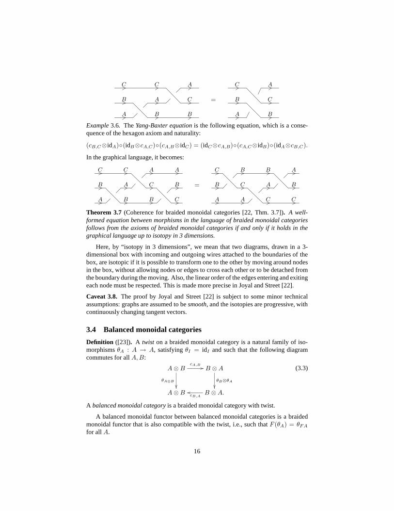
Example3.6. TheYang-Baxter equationis the following equation, which is a conse-quence of the hexagon axiom and naturality:

(cB,C⊗idA)◦(idB⊗cA,C)◦(cA,B⊗idC) = (idC⊗cA,B)◦(cA,C⊗idB)◦(idA⊗cB,C).

In the graphical language, it becomes:

C C A A

B A C B

A B B C

=

C B B A

B C A B

A A C C

Theorem 3.7 (Coherence for braided monoidal categories [22, Thm. 3.7]). A well-formed equation between morphisms in the language of braided monoidal categoriesfollows from the axioms of braided monoidal categories if and only if it holds in thegraphical language up to isotopy in 3 dimensions.

Here, by “isotopy in 3 dimensions”, we mean that two diagrams, drawn in a 3-dimensional box with incoming and outgoing wires attached to the boundaries of thebox, are isotopic if it is possible to transform one to the other by moving around nodesin the box, without allowing nodes or edges to cross each other or to be detached fromthe boundary during the moving. Also, the linear order of theedges entering and exitingeach node must be respected. This is made more precise in Joyal and Street [22].

Caveat 3.8. The proof by Joyal and Street [22] is subject to some minor technicalassumptions: graphs are assumed to besmooth, and the isotopies are progressive, withcontinuously changing tangent vectors.

3.4 Balanced monoidal categories

Definition ([23]). A twist on a braided monoidal category is a natural family of iso-morphismsθA : A → A, satisfyingθI = idI and such that the following diagramcommutes for allA, B:

A ⊗ B

θA⊗B

cA,B

B ⊗ A

θB⊗θA

A ⊗ B B ⊗ A.cB,A

(3.3)

A balanced monoidal categoryis a braided monoidal category with twist.

A balanced monoidal functor between balanced monoidal categories is a braidedmonoidal functor that is also compatible with the twist, i.e., such thatF (θA) = θFA

for all A.

16

Graphical language. The graphical language of balanced monoidal categories issimilar to that of braided monoidal categories, except thatmorphisms are representedby flat ribbons, rather than 1-dimensional wires. A ribbon can be thought of as a pair ofparallel wires that are infinitesimally close to each other,or as a wire that is equippedwith a framing[22]. For example, the braiding looks like this:

cA,B = .

The twist mapθA is represented as a 360-degree twist in a ribbon, or in several rib-bons together, ifA is a composite object term. This is easiest seen in the followingillustration.

θA = , θA⊗B = .

The meaning of (3.3) should then be obvious.

Theorem 3.9(Coherence for balanced monoidal categories [22, Thm. 4.5]). A well-formed equation between morphisms in the language of balanced monoidal categoriesfollows from the axioms of balanced monoidal categories if and only if it holds in thegraphical language up to framed isotopy in 3 dimensions.

3.5 Symmetric monoidal categories

Definition. A symmetric monoidal categoryis a braided monoidal category where thebraiding is self-inverse, i.e.:

cA,B = c−1B,A

In this case, the braiding is called asymmetry.

Remark3.10. Because of equation (3.3), a symmetric monoidal category can be equiv-alently defined as a balanced monoidal category in whichθA = idA for all A.

Remark3.11. The previous remark notwithstanding, there exist symmetric monoidalcategories that possess a non-trivial twist (in addition tothe trivial twist θA = idA).Thus, in a balanced monoidal category, the symmetry condition cA,B = c−1

B,A doesnot in general implyθA = idA. In other words, a balanced monoidal category that issymmetric as a braided monoidal category is not necessarilysymmetric as a balancedmonoidal category. An example is the category of finite dimensional vector spaces andlinear bijections, withθA(x) = nx, wheren = dim(A).

Examples. On the monoidal category(Set,×) of sets with cartesian product, a sym-metry is given byc(x, y) = (y, x). On the category(Vect,⊗) of vector spaces withtensor product, a symmetry is given byc(x ⊗ y) = y ⊗ x.

17

Graphical language. The symmetry is graphically represented by a crossing:

Symmetry cA,B

B A

A B

Theorem 3.12(Coherence for symmetric monoidal categories [22, Thm. 2.3]). A well-formed equation between morphisms in the language of symmetric monoidal categoriesfollows from the axioms of symmetric monoidal categories ifand only if it holds, up toisomorphism of diagrams, in the graphical language.

Note that the graphical language for symmetric monoidal categories is up to iso-morphism of diagrams, without any reference to 2- or 3-dimensional structure. How-ever, isomorphism of diagrams is equivalent to ambient isotopy in 4 dimensions, so wecan still regard it as a geometric notion.

4 Autonomous categories

Autonomous categories are monoidal categories in which theobjects haveduals. Interms of graphical language, this means that some wires are allowed to run from rightto left.

4.1 (Planar) autonomous categories

Definition ([23]). In a (without loss of generality strict) monoidal category,anexactpairing between two objectsA andB is given by a pair of morphismsη : I → B ⊗ A

andǫ : A ⊗ B → I, such that the following two adjunction triangles commute:

AidA⊗η

idA

A ⊗ B ⊗ A

ǫ⊗idA

A,

Bη⊗idB

idB

B ⊗ A ⊗ B

idB⊗ǫ

B.

(4.1)

In such an exact pairing,B is called theright dualof A andA is called theleft dualofB.

Remark4.1. The mapsη andǫ determine each other uniquely, and they are respectivelycalled theunit and thecounit of the adjunction. Moreover, the triple(B, η, ǫ), if itexists, is uniquely determined byA up to isomorphism. The existence of duals istherefore a property of a monoidal category, rather than an additional structure on it.Moreover, every strong monoidal functor automatically preserves existing duals.

Definition ([20, 21, 23]). A monoidal category isright autonomousif every objectAhas a right dual, which we then denoteA∗. It is left autonomousif every objectA hasa left dual, which we then denote∗A. Finally, the category isautonomousif it is bothright and left autonomous.

18

Remark4.2 (Terminology). A [right, left, –] autonomous category is also called [right,left, –] rigid, see e.g. [32, p. 78]. Also, the term “autonomous” is sometimes used in theweaker sense of “monoidal closed”. Although this latter usage is no longer common, itstill lives on in the terminology “*-autonomous category” (Barr [4], see also Section 9).

If we wish to emphasize that an autonomous category is not necessarily symmetricor braided, we sometimes call it aplanar autonomous category.

Graphical language. If A is an object variable, the objectsA∗ and∗A are both rep-resented in the same way: by a wire labeledA running from right to left. The unit andcounit are represented as half turns:

Dual A∗, ∗AA

Unit ηA : I → A∗ ⊗ AA

Aη′

A : I → A ⊗ ∗AA

A

Counit ǫA : A ⊗ A∗ → IA

Aǫ′A : ∗A ⊗ A → I

A

A

More generally, ifA is a composite object represented by a number of wires, thenA∗ and∗A are represented by the same set of wires running backward (rotated by 180degrees), and the units and counits are represented as multiple wires turning.

Example4.3. The two diagrams in (4.1), whereB = A∗, translate into the graphicallanguage as follows:

A

A

A

=A

,

A

A

A

=A

.

Example4.4. For any morphismf : A → B, it is possible to define morphismsf∗ : B∗ → A∗ and∗f : ∗B → ∗A, called theadjoint matesof f , as follows:

f∗ =

B

Af

B

A

∗f =

A

Af

B

B

With these definitions,(−)∗ and∗(−) become contravariant functors.

Theorem 4.5(Coherence for planar autonomous categories [21, Thm. 2.7]). A well-formed equation between morphisms in the language of autonomous categories followsfrom the axioms of autonomous categories if and only if it holds in the graphical lan-guage up to planar isotopy.

19

Here, the notion of planar isotopy is the same as before, except that the wires areof course no longer restricted to being oriented left-to-right during the deformation.However, the ability to turn wires upside down does not extend to boxes: the notionof isotopy for this theorem does not include the ability to rotate boxes. See Joyal andStreet [21] for a more precise statement.

Caveat 4.6.The proof by Joyal and Street [21] assumes that the diagrams are piecewiselinear.

Note that the same theorem applies to left autonomous, rightautonomous, or au-tonomous categories. Indeed, each individual term in the language of autonomouscategories involves only finitely many duals, and thus may betranslated into a term of(say) left autonomous categories by replacing each object variableA by A∗∗∗...∗, for asufficiently large, even number of∗’s. The resulting term maps to the same diagram.

The same coherence theorem also holds for categories that are only right (or left)autonomous. This is a consequence of the following proposition.

Proposition 4.7. Each right (or left) autonomous category can be fully embedded inan autonomous category.

Proof. LetC be a right autonomous category, and consider the strong monoidal functorF : C → C given byF (A) = A∗∗. This functor is full and faithful, and every objectin the image ofF has a left dual. Now letC be the colimit (in the large category ofright autonomous categories and strong monoidal functors)of the sequence

CF−→ C

F−→ C

F−→ . . .

ThenC is autonomous, andC is fully and faithfully embedded inC. The proof forleft autonomous categories is analogous. 2

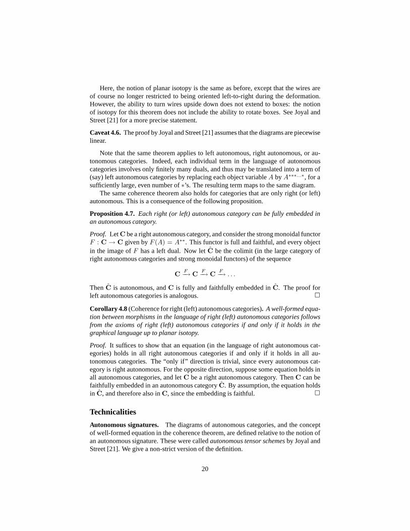
Corollary 4.8 (Coherence for right (left) autonomous categories). A well-formed equa-tion between morphisms in the language of right (left) autonomous categories followsfrom the axioms of right (left) autonomous categories if andonly if it holds in thegraphical language up to planar isotopy.

Proof. It suffices to show that an equation (in the language of right autonomous cat-egories) holds in all right autonomous categories if and only if it holds in all au-tonomous categories. The “only if” direction is trivial, since every autonomous cat-egory is right autonomous. For the opposite direction, suppose some equation holds inall autonomous categories, and letC be a right autonomous category. ThenC can befaithfully embedded in an autonomous categoryC. By assumption, the equation holdsin C, and therefore also inC, since the embedding is faithful. 2

Technicalities

Autonomous signatures. The diagrams of autonomous categories, and the conceptof well-formed equation in the coherence theorem, are defined relative to the notion ofan autonomous signature. These were calledautonomous tensor schemesby Joyal andStreet [21]. We give a non-strict version of the definition.

20

Definition. [21, Def. 2.5] Given a setΣ0 of object variables, let Aut(Σ0) denote thefree(⊗, I, ∗(−), (−)∗)-algebra generated byΣ0, i.e., the set ofobject termsbuilt fromobject variables andI via the operations⊗, ∗(−), and(−)∗). For example, ifA, B ∈Σ0, then the termB∗ ⊗ (∗∗I ⊗ A)∗ is an element of Aut(Σ0).

An autonomous signatureconsists of a setΣ0 of object variables, a setΣ1 of mor-phism variables, and a pair of functions dom, cod : Σ1 → Aut(Σ0).

The concept of aright autonomous signatureand left autonomous signaturearedefined analogously. The remaining graphical languages in this Section 4 are all givenrelative to an autonomous signature.

Functors and natural transformations of autonomous categories. Any strong monoidalfunctor preserves exact pairings: ifη : I → B ⊗ A andǫ : A⊗B → I define an exactpairing, then so do

F η : Iφ0

−→ FIFη−−→ F (B ⊗ A)

(φ2)−1

−−−−→ FB ⊗ FA

and

F ǫ : FA ⊗ FBφ2

−→ F (A ⊗ B)Fǫ−−→ FI

(φ0)−1

−−−−→ I.

In particular, ifC andD are autonomous categories andF : C → D is a monoidalfunctor, by uniqueness of duals, there will be a unique induced natural isomorphismF (A∗) ∼= (FA)∗ such that

I

ηF A

F ηA

F (A∗) ⊗ FA

∼=⊗id

(FA)∗ ⊗ FA

and

FA ⊗ F (A∗)

id⊗∼=

F ǫAI,

FA ⊗ (FA)∗

ǫF A

and similarly forF (∗A) ∼= ∗(FA).For natural transformations, we have the following lemma:

Lemma 4.9 (Saavedra Rivano [32, Prop. 5.2.3], see also [23, Prop. 7.1]). Supposeτ : F → G is a monoidal natural transformation between strong monoidal functorsF, G : C → D. If A has a right dualA∗ in C, thenτA∗ and(τA)∗ are mutually inversein D (up to the above canonical isomorphism), or more precisely:

F (A∗)τA∗

∼=

G(A∗)

∼=

(FA)∗ (GA)∗(τA)∗

In particular, if C is autonomous, then any such monoidal natural transformation isinvertible.

21

Coherence and free autonomous categories.The graphical language, as we havedefined it above for autonomous categories, is sufficient forthe purposes of Theo-rem 4.5. However, it does not characterize the free autonomous category over an au-tonomous signature as stated. For example, consider a signature with a single mor-phism variablef : A → A. The problem is that there are clearly some diagrams, suchas

Af

A (4.2)

which are not translations of any well-formed term of autonomous categories. Indeed,for this diagram to correspond to a well-formed term, we would have to have e.g.f :A∗∗ → A or f : A → ∗∗A.

Joyal and Street [21] characterize the free autonomous category by equipping eachedge with a winding number. Effectively, the horizontal segments of edges are labeledwith pairs(A, n), whereA is an object variables andn is an integer winding number.Left-to-right segments have even winding numbers, right-to-left segments have oddwinding numbers, and winding numbers increase by one on counterclockwise turns,and decrease by one on clockwise turns. The winding numbers on the input and outputof each box, and on the global inputs and outputs, are restricted to be consistent withthe domain and codomain information, where e.g.A∗∗ corresponds to(A, 2), and∗∗∗B

to (B,−3). See [21] for precise details. Here is an example of a well-formed diagramof typeI → B∗∗ ⊗ A, whereg : I → A ⊗ B:

( ,1)B

( ,0)B

A( ,0)

( ,2) B

g

Theorem 4.10. The graphical language (with winding numbers) of autonomous cate-gories over an autonomous signatureΣ, up to planar isotopy of diagrams, forms a freeautonomous category overΣ.

We remark that if a diagram of planar autonomous categories can be labeled withwinding numbers, then this labeling is necessarily unique.In particular, for the pur-poses of Theorem 4.5, there is no harm in dropping the windingnumbers, because byhypothesis, the theorem only considers diagrams that are the translation of well-formedterms, whose winding numbers can therefore uniquely reconstructed.

4.2 (Planar) pivotal categories

A pivotal category is an autonomous category with a suitableisomorphismA ∼= A∗∗.

Definition ([15, 16, 19]). A pivotal categoryis a right autonomous category equippedwith a monoidal natural isomorphismiA : A → A∗∗.

22

Note that any pivotal category is immediately left autonomous, therefore autonomous.The requirement thatiA is amonoidalnatural transformation here means thatiI is thecanonical isomorphismI ∼= I∗∗, and that the following diagram commutes, where thehorizontal arrow is the canonical isomorphism derived fromthe autonomous structure:

A ⊗ B

iA⊗iB iA⊗B

A∗∗ ⊗ B∗∗∼=

(A ⊗ B)∗∗.

(4.3)

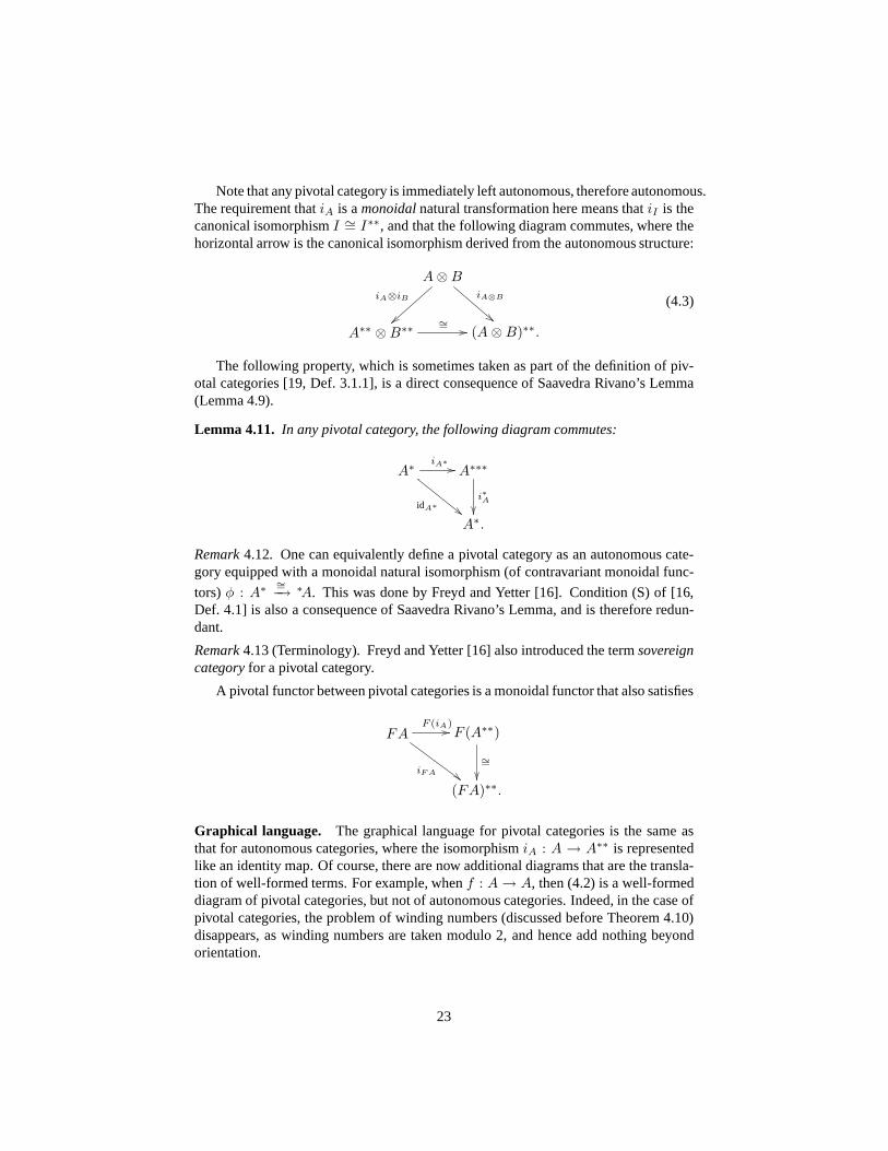
The following property, which is sometimes taken as part of the definition of piv-otal categories [19, Def. 3.1.1], is a direct consequence ofSaavedra Rivano’s Lemma(Lemma 4.9).

Lemma 4.11. In any pivotal category, the following diagram commutes:

A∗iA∗

idA∗

A∗∗∗

i∗A

A∗.

Remark4.12. One can equivalently define a pivotal category as an autonomous cate-gory equipped with a monoidal natural isomorphism (of contravariant monoidal func-

tors)φ : A∗∼=−→ ∗A. This was done by Freyd and Yetter [16]. Condition (S) of [16,

Def. 4.1] is also a consequence of Saavedra Rivano’s Lemma, and is therefore redun-dant.

Remark4.13 (Terminology). Freyd and Yetter [16] also introduced the termsovereigncategoryfor a pivotal category.

A pivotal functor between pivotal categories is a monoidal functor that also satisfies

FAF (iA)

iF A

F (A∗∗)

∼=

(FA)∗∗.

Graphical language. The graphical language for pivotal categories is the same asthat for autonomous categories, where the isomorphismiA : A → A∗∗ is representedlike an identity map. Of course, there are now additional diagrams that are the transla-tion of well-formed terms. For example, whenf : A → A, then (4.2) is a well-formeddiagram of pivotal categories, but not of autonomous categories. Indeed, in the case ofpivotal categories, the problem of winding numbers (discussed before Theorem 4.10)disappears, as winding numbers are taken modulo 2, and henceadd nothing beyondorientation.

23

Theorem 4.14(Coherence for pivotal categories). A well-formed equation betweenmorphisms in the language of pivotal categories follows from the axioms of pivotalcategories if and only if it holds in the graphical language up to planar isotopy, includ-ing rotation of boxes.

Caveat 4.15. Only special cases of this theorem have been proved in the literature.Freyd and Yetter [16, Thm. 4.4] considered the case of the free pivotal category gener-ated by a category. In our terminology, this means that they only considered diagramsfor pivotal categories oversimple signatures, rather than overautonomous signatures.In other words, they only considered boxes of the form

Af

B,

with exactly one input and one output. Joyal and Street’s draft report [19] claims thegeneral result but contains no proof.

The notion of planar isotopy for pivotal categories includes the ability to rotateboxes in the plane of the diagram. For example, the followingtwo diagrams are isotopicin this sense:

f = f (4.4)

This also explains why we have marked a corner of each box. With the ability to rotateboxes, we need to keep track of their “natural” orientation,so that the diagrams from(4.4) can also be represented like this:

f

More generally, the adjoint mate off : A → B can be represented by a rotated box:

f∗ =

B

Af

B

A

=B

fA (4.5)

Also note that isf is a composite diagram, then the whole diagram may be rotatedtoobtainf∗.

24

4.3 Spherical pivotal categories

Definition (Barrett and Westbury [5]). A pivotal category issphericalif for all objectsA and morphismsf : A → A,

Af

A =A

fA

(4.6)

The intuition behind the “spherical” axioms is that diagrams should be embeddedin a 2-sphere, rather than the plane. It is then obvious that the left-hand side of (4.6)can be continuously transformed into the right-hand side, namely by moving the loopacross the back of the 2-sphere.

Failure of coherence. The spherical axiom is not sound for the graphical languageof diagrams embedded in the 2-sphere. The problem is that thenotion of “diagramembedded in the 2-sphere” is not compatible with composition or tensor. The followingis a consequence of the spherical axiom, but does not hold up to isotopy in the 2-sphere.

g

Af

A

=

g

Af

A =

g

Af

A

Note that this counterexample is similar to the spacial axiom (3.2), but does not quiteimply it. If one adds the spacial axiom, as we are about to do, then any notion ofisotopy is lost and equivalence of diagrams collapses to isomorphism.

4.4 Spacial pivotal categories

Definition. A pivotal category isspacialif it satisfies the spacial axiom (3.2) and thespherical axiom (4.6).

Graphical language and coherence. The graphical language for spacial pivotal cat-egories is the same as that for planar pivotal categories, except that equivalence of dia-grams is now taken up to isomorphism. Clearly, the axioms aresound for the graphicallanguage. We conjecture that they are also complete.

Conjecture 4.16(Coherence for spacial pivotal categories). A well-formed equationbetween morphisms in the language of spacial pivotal categories follows from the ax-ioms of spacial pivotal categories if and only if it holds in the graphical language upto isomorphism.

25

4.5 Braided autonomous categories

An braided autonomous category is an autonomous category that is also braided (as amonoidal category). The notion of braided autonomous categories is not extremely nat-ural, as the graphical language is only sound for a restricted form of isotopy calledreg-ular isotopy. Nevertheless, it is useful to collect some facts about braided autonomouscategories.

Lemma 4.17([23, Prop. 7.2]). A braided monoidal category is autonomous if and onlyif it is right autonomous.

Proof. If η : I → B ⊗ A andǫ : A ⊗ B → I form an exact pairing, then so doc−1A,B ◦ η : I → A ⊗ B andǫ ◦ cB,A : B ⊗ A → I. Therefore any right dual ofA is

also a left dual ofA. 2

In any braided autonomous categoryC, we can define a natural isomorphismbA :A∗∗ → A. This follows from the proof of Lemma 4.17, using the fact that bothA andA∗∗ are right duals ofA∗. More concretely,bA and its inverse are defined by:

bA = A∗∗ ηA⊗id−−−−→ A∗ ⊗ A ⊗ A∗∗

id⊗cA,A∗∗−−−−−−→ A∗ ⊗ A∗∗ ⊗ A

ǫA∗⊗id−−−−→ A,

b−1A = A

id⊗ηA∗−−−−→ A ⊗ A∗∗ ⊗ A∗

c−1

A∗∗,A⊗id

−−−−−−→ A∗∗ ⊗ A ⊗ A∗ id⊗ǫA−−−−→ A∗∗.

Here we have written, without loss of generality, as ifC were strict monoidal. Graphi-cally, bA and its inverse look like this:

bA =

A∗∗ A

A∗

b−1A =

A∗

A A∗∗

We must note that althoughbA is a natural isomorphism, it is not canonical. In general,there exist infinitely many natural isomorphismsA ∼= A∗∗. Also, b is not amonoidalnatural transformation, and therefore does not define a pivotal structure onC. A gen-eral braided autonomous category is not pivotal.

Graphical language and coherence. The graphical language braided autonomouscategories is obtained simply by adding braids to the graphical language of autonomouscategories. However, the correct notion of equivalence of diagrams is neither planarisotopy (like for autonomous categories), nor 3-dimensional isotopy (like for braidedmonoidal categories), but an in-between notion calledregular isotopy[25].

It is well-known that 3-dimensional isotopy of links and tangles is equivalent toplanar isotopy of their (non-degenerate) projections ontoa 2-dimensional plane, plusthe threeReidemeister moves[31] shown as (R1)–(R3) in Figure 3. To extend this todiagrams with nodes, one also has to add the moves (Λ1) and (Λ2).

Regular isotopyis defined to be the equivalence obtained by dropping Reidemeistermove (R1). Note that regular isotopy is an equivalence on 2-dimensional representationof 3-dimensional diagrams (and not of 3-dimensional diagrams themselves).

26

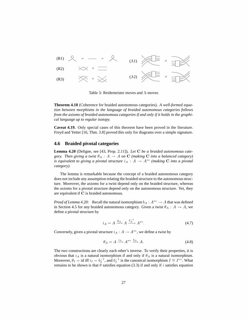
(R1) = =

(R2) =

(R3) =

(Λ1) =... ...

... ...

(Λ2) =... ...

... ...

Table 3: Reidemeister moves andΛ-moves

Theorem 4.18(Coherence for braided autonomous categories). A well-formed equa-tion between morphisms in the language of braided autonomous categories followsfrom the axioms of braided autonomous categories if and onlyif it holds in the graphi-cal language up to regular isotopy.

Caveat 4.19. Only special cases of this theorem have been proved in the literature.Freyd and Yetter [16, Thm. 3.8] proved this only for diagramsover a simple signature.

4.6 Braided pivotal categories

Lemma 4.20(Deligne, see [43, Prop. 2.11]). Let C be a braided autonomous cate-gory. Then giving a twistθA : A → A on C (makingC into a balanced category)is equivalent to giving a pivotal structureiA : A → A∗∗ (makingC into a pivotalcategory).

The lemma is remarkable because the concept of a braided autonomous categorydoes not include any assumption relating the braided structure to the autonomous struc-ture. Moreover, the axioms for a twist depend only on the braided structure, whereasthe axioms for a pivotal structure depend only on the autonomous structure. Yet, theyare equivalent ifC is braided autonomous.

Proof of Lemma 4.20:Recall the natural isomorphismbA : A∗∗ → A that was definedin Section 4.5 for any braided autonomous category. Given a twist θA : A → A, wedefine a pivotal structure by

iA = AθA−−→ A

b−1

A−−→ A∗∗. (4.7)

Conversely, given a pivotal structureiA : A → A∗∗, we define a twist by

θA = AiA−→ A∗∗ bA−−→ A. (4.8)

The two constructions are clearly each other’s inverse. To verify their properties, it isobvious thatiA is a natural isomorphism if and only ifθA is a natural isomorphism.Moreover,θI = id iff iI = b−1

I , andb−1I is the canonical isomorphismI ∼= I∗∗. What

remains to be shown is thatθ satisfies equation (3.3) if and only ifi satisfies equation

27

(4.3). However, this is a direct consequence of the following fact aboutb, which iseasily verified:

A∗∗ ⊗ B∗∗

∼=

cA,B

B∗∗ ⊗ A∗∗

bB⊗bA(A ⊗ B)∗∗

bA⊗B

A ⊗ B B ⊗ A.cB,A

2

Corollary 4.21. A braided pivotal category is the same thing as a balanced autonomouscategory. 2

Remark4.22. While Lemma 4.20 establishes a one-to-one correspondence betweentwists and pivotal structures, the correspondence is not canonical. Indeed, instead of(4.7) and (4.8), we could have equally well used

iA = Aθ−1

A−−→ Ab′A−−→ A∗∗ (4.9)

and

θA = Ab′A−−→ A∗∗ i

−1

A−−→ A, (4.10)

whereb′A = A A** .

In fact, there are a countable number of such similar one-to-one correspondences, allinduced by the existence of a monoidal natural transformation b′A

−1 ◦ iA ◦ bA ◦ iA :A → A. They all coincide if and only if the category is tortile, as discussed in the nextsection.

Graphical language and coherence. The graphical language for braided pivotal cat-egories is the same as the graphical language for pivotal categories, with the addition ofbraids. Equivalence of diagrams is up to regular isotopy, just as for braided autonomouscategories (see Section 4.5).

Theorem 4.23(Coherence for braided pivotal categories). A well-formed equation be-tween morphisms in the language of braided pivotal categories follows from the axiomsof braided pivotal categories if and only if it holds in the graphical language up to reg-ular isotopy.

Caveat 4.24. Only special cases of this theorem have been proved in the literature.Freyd and Yetter [16, Thm. 4.4] proved this only for diagramsover a simple signature.

Remark4.25. The equation

=

28

holds up to regular isotopy, as it can be proved using only theReidemeister moves (R2)and (R3). It is therefore valid in braided pivotal categories (or even braided autonomouscategories). On the other hand, the equation

=

holds up to isotopy, but not up to regular isotopy (because regular isotopy preservestotal curvature, as pointed out by Freyd and Yetter [15, p. 169]). It is therefore notvalid in braided pivotal categories. The use of regular isotopy does not seem natural,and this is precisely the reason why Joyal and Street introduced tortile categories, whichwe discuss in the next section.

Remark4.26. A braided pivotal category is not in general spherical (and therefore alsonot spacial). Indeed, instead of the spherical axiom (4.6),only the following holds upto regular isotopy:

f f=

Along with Remark 4.22, this is further evidence that braided pivotal categories (andbraided autonomous categories) are not “natural” notions.

4.7 Tortile categories

Lemma 4.27. Consider a braided pivotal category, which is equivalentlybalancedautonomous via (4.7) and (4.8). For any objectA the following are equivalent:

(a) (ǫA∗ ⊗ idA)◦(idA∗⊗c−1A∗∗,A)◦(ηA⊗ idA∗∗)◦iA◦(ǫA∗⊗ idA)◦(idA∗⊗cA,A∗∗)◦

(ηA ⊗ idA∗∗) ◦ iA = idA, or graphically:

= AA AA

(b) θA∗ = (θA)∗.

Proof. The proof is a straightforward calculation, but it is best explained by the factthat the following hold in the graphical language:

θA = A A (θA)∗ = *A *A θA∗ = *A *A (θA∗)−1 = *A *A .

Therefore, the equation (b) is equivalent to

*A *A *A*A=

,

which is the adjoint mate of (a). 2

29

Remark4.28. The condition in Lemma 4.27(a) holds if and only if the two definitionsof θA from (4.8) and (4.10) coincide.

Definition ([23]). A tortile categoryis a braided pivotal category satisfying the con-dition of Lemma 4.27(a). Equivalently, a tortile category is a balanced autonomouscategory satisfying the condition of Lemma 4.27(b).

Remark4.29 (Terminology). A tortile category is also sometimes called aribbon cat-egory, see e.g. [42].

Graphical language and coherence. The graphical language for tortile categoriesis like the graphical language for braided pivotal categories, except that morphismsare represented by ribbons, rather than wires. These ribbons are just like the ones forbalanced categories from Section 3.4. Units and counits arerepresented in the obviousway, for example

ηA = , ǫA = .

The twist mapθA : A → A can be represented in several equivalent ways:

θA = = = .

Note that these diagrams are equivalent up to framed 3-dimensional isotopy, and definethe same morphism in a tortile category. (On the other hand, in a mere braided piv-otal category, the latter two diagrams are not equal). Also note that the mapbA fromSection 4.5 is also represented in the graphical language as

bA = ,

but this is of typebA : A∗∗ → A, whereasθA : A → A. They differ, of course, onlyby an invisible pivotal mapiA : A → A∗∗.

Theorem 4.30(Coherence for tortile categories). A well-formed equation betweenmorphisms in the language of tortile categories follows from the axioms of tortile cat-egories if and only if it holds in the graphical language up toframed 3-dimensionalisotopy.

Caveat 4.31. Only special cases of this theorem have been proved in the literature.Shum [34, Thm. 6.1] proved it for the case of the free tortile category generated by acategory, i.e., for diagrams over a simple signature only.

4.8 Compact closed categories

A compact closed category is a tortile category that is symmetric (as a balanced monoidalcategory) in the sense of Section 3.5. Equivalently, because of Remark 3.10, a compactclosed category is a tortile category in whichθA = idA for all A.

30

The definition can be simplified. Notice that a right autonomous symmetric monoidalcategory is automatically autonomous (by Lemma 4.17), balanced (withθA = idA) andtherefore pivotal (by Lemma 4.20). Moreover, it is tortile (becauseθA∗ = (θA)∗ =idA∗ ). We can therefore define:

Definition. A compact closed categoryis a right autonomous symmetric monoidalcategory.

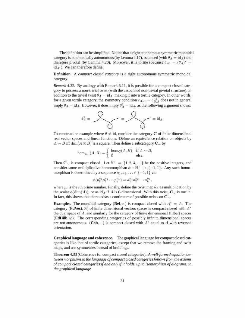
Remark4.32. By analogy with Remark 3.11, it is possible for a compact closed cate-gory to possess a non-trivial twist (with the associated non-trivial pivotal structure), inaddition to the trivial twistθA = idA, making it into a tortile category. In other words,for a given tortile category, the symmetry conditioncA,B = c−1

B,A does not in generalimply θA = idA. However, it does implyθ2

A = idA, as the following argument shows:

θ2A = = = idA.

To construct an example whereθ 6= id, consider the categoryC of finite-dimensionalreal vector spaces and linear functions. Define an equivalence relation on objects byA ∼ B iff dim(A ⊗ B) is a square. Then define a subcategoryC∼ by

homC∼(A, B) =

{

homC(A, B) if A ∼ B,∅ else.

ThenC∼ is compact closed. LetN+ = {1, 2, 3, . . .} be the positive integers, andconsider some multiplicative homomorphismφ : N

+ → {−1, 1}. Any such homo-morphism is determined by a sequencea1, a2, . . . ∈ {−1, 1} via

φ(pn1

1 pn2

2 · · · pnk

k ) = an1

1 an2

2 · · · ank

k ,

wherepi is theith prime number. Finally, define the twist mapθA as multiplication bythe scalarφ(dim(A)), or as idA if A is 0-dimensional. With this twist,C∼ is tortile.In fact, this shows that there exists a continuum of possibletwists onC∼.

Examples. The monoidal category(Rel,×) is compact closed withA∗ = A. Thecategory(FdVect,⊗) of finite dimensional vectors spaces is compact closed withA∗

the dual space ofA, and similarly for the category of finite dimensional Hilbert spaces(FdHilb ,⊗). The corresponding categories of possibly infinite dimensional spacesare not autonomous.(Cob, +) is compact closed withA∗ equal toA with reversedorientation.

Graphical language and coherence. The graphical language for compact closed cat-egories is like that of tortile categories, except that we remove the framing and twistmaps, and use symmetries instead of braidings.

Theorem 4.33(Coherence for compact closed categories). A well-formed equation be-tween morphisms in the language of compact closed categories follows from the axiomsof compact closed categories if and only if it holds, up to isomorphism of diagrams, inthe graphical language.

31

(a)

f

(b)

f

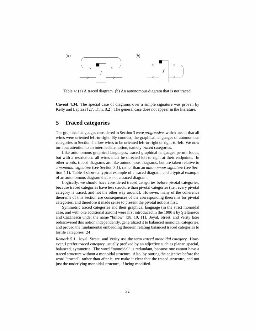
Table 4: (a) A traced diagram. (b) An autonomous diagram thatis not traced.

Caveat 4.34. The special case of diagrams over a simple signature was proven byKelly and Laplaza [27, Thm. 8.2]. The general case does not appear in the literature.

5 Traced categories

The graphical languages considered in Section 3 wereprogressive, which means that allwires were oriented left-to-right. By contrast, the graphical languages of autonomouscategories in Section 4 allow wires to be oriented left-to-right or right-to-left. We nowturn out attention to an intermediate notion, namelytracedcategories.

Like autonomous graphical languages, traced graphical languages permit loops,but with a restriction: all wires must be directed left-to-right at their endpoints. Inother words, traced diagrams are like autonomous diagrams,but are taken relative toa monoidal signature(see Section 3.1), rather than anautonomous signature(see Sec-tion 4.1). Table 4 shows a typical example of a traced diagram, and a typical exampleof an autonomous diagram that is not a traced diagram.

Logically, we should have considered traced categories before pivotal categories,because traced categories have less structure than pivotalcategories (i.e., every pivotalcategory is traced, and not the other way around). However, many of the coherencetheorems of this section are consequences of the corresponding theorems for pivotalcategories, and therefore it made sense to present the pivotal notions first.

Symmetric traced categories and their graphical language (in the strict monoidalcase, and with one additional axiom) were first introduced inthe 1980’s by Stefanescuand Cazanescu under the name “biflow” [38, 10, 11]. Joyal, Street, and Verity laterrediscovered this notion independently, generalized it tobalanced monoidal categories,and proved the fundamental embedding theorem relating balanced traced categories totortile categories [24].

Remark5.1. Joyal, Street, and Verity use the termtraced monoidal category. How-ever, I prefertraced category, usually prefixed by an adjective such as planar, spacial,balanced, symmetric. The word “monoidal” is redundant, because one cannot have atraced structure without a monoidal structure. Also, by putting the adjective before theword “traced”, rather than after it, we make it clear that thetraced structure, and notjust the underlying monoidal structure, if being modified.

32

5.1 Right traced categories

Definition. A right traceon a monoidal category is a family of operations

TrXR : hom(A ⊗ X, B ⊗ X) → hom(A, B),

satisfying the following four axioms. For notational convenience, we assume withoutloss of generality that the monoidal structure is strict.

(a) Tightening (naturality inA, B): TrXR ((g⊗ idX)◦f ◦(h⊗ idX)) = g◦(TrXR f)◦h;

(b) Sliding (dinaturality inX): TrYR (f ◦ (idA ⊗ g)) = TrXR ((idB ⊗ g) ◦ f), wheref : A ⊗ X → B ⊗ Y andg : Y → X ;

(c) Vanishing: TrIR f = f and TrX⊗YR f = TrXR (TrYR (f));

(d) Strength. TrXR (g ⊗ f) = g ⊗ TrXR f .

A (planar) right traced categoryis a monoidal category equipped with a right trace.

These axioms are similar to those of Joyal, Street, and Verity [24], except that wehave omitted the yanking axioms which does not apply in the planar case, and we havereplaced the non-planar “superposing” axiom by the planar “strength” axiom. I do notknow whether this set of planar axioms appears in the literature.

Graphical language and coherence. The right trace of a diagramf : A ⊗ X →B ⊗X is graphically represented by drawing a loop from the outputX to the inputX ,as follows:

TrXR f =X X

Af

B

(5.1)

Note that in the graphical language of right traced categories, parts of wires can beoriented right-to-left, but each wire must be oriented left-to-right near the endpoints.The four axioms of right traced categories are illustrated in the graphical language inTable 5. The axioms of right traced categories are obviouslysound for the graphicallanguage, up to planar isotopy. We conjecture that they are also complete.

Conjecture 5.2 (Coherence for right traced categories). A well-formed equation be-tween morphism terms in the language of right traced categories follows from the ax-ioms of right traced categories if and only if it holds in the graphical language upplanar isotopy.

This is a weak conjecture, in the sense that there is not much empirical evidence tosupport it, nor is there an obvious strategy for a proof. If this conjecture turns out to befalse, the axioms for right traced categories should be amended until it becomes true.

33

Table 5: The axioms of right traced categories

The concept of aleft traceis defined similarly as a family of operations

TrXL : hom(X ⊗ A, X ⊗ B) → hom(A, B),

satisfying symmetric axioms. A left trace is graphically depicted as follows:

TrXL g =

A B

Xg

X (5.2)

We say that a monoidal functorF preserves right tracesif F (TrXR f) = TrFXR ((φ2)−1◦

Ff ◦ φ2), and similarly for left traces.

5.2 Planar traced categories

Definition. A planar traced categoryis a monoidal category equipped with a righttrace and a left trace, such that the two traces satisfy threeadditional axioms:

(a) Interchange: TrXR (TrYL f) = TrYL (TrXR f), for all f : Y ⊗A⊗X → Y ⊗B⊗X ;

(b) Left pivoting: TrBR (idB ⊗ f) = TrAL (f ⊗ idA), for all f : I → A ⊗ B;

(c) Right pivoting: TrBR (idB ⊗ f) = TrAL (f ⊗ idA), for all f : A ⊗ B → I.

Graphical language and coherence. The graphical language of planar traced cate-gories consists of diagrams using the left and right trace together, modulo planar iso-topy. The axioms of interchange, left pivoting, and right pivoting are shown graphicallyin Table 6. Compare also equation (4.4) on page 4.4. The axioms are clearly sound;we conjecture that they are also complete:

34

= = =

(a) interchange (b) left pivoting (c) right pivoting

Table 6: Axioms relating left and right trace

Conjecture 5.3(Coherence for planar traced categories). A well-formed equation be-tween morphism terms in the language of planar traced categories follows from theaxioms of planar traced categories if and only if it holds in the graphical language upplanar isotopy.

As for right traced categories, this conjecture is weak. If it turns out to be false,then one should amend the axioms of planar traced categoriesaccordingly.

Remark5.4. Even if the conjecture is true, the graphical language does not in itselfgive an easy description of the free planar traced category.This is because there arediagrams, such as the following, that “look” planar traced,but are not actually thediagram of any planar traced term (not even up to planar isotopy).

It is not obvious how to characterize the “planar traced” diagrams intrinsically, or howto extend the notion of planar traced categories to encompass all such diagrams.

Remark5.5. An autonomous category is not necessarily traced. However,every pivotalcategory is planar traced with the obvious definitions of left and right trace:

TrXR f = (idB ⊗ ǫX) ◦ ((f ◦ (idA ⊗ i−1X )) ⊗ idX∗) ◦ (idA ⊗ ηX∗),

TrXL f = (ǫX∗ ⊗ idB) ◦ (idX∗ ⊗ ((iX ⊗ idB) ◦ f)) ◦ (ηX ⊗ idA).

In the graphical language, this looks just like the diagrams(5.1) and (5.2). As a con-sequence, each diagram of planar traced categories can be regarded as a diagram ofplanar pivotal categories, but not the other way around.

5.3 Spherical traced categories

The concept of a spherical traced category is analogous to that of spherical pivotalcategories from Section 4.3.

Definition. A planar traced category satisfies thespherical axiomif for all f : A → A,

TrAL f = TrAR f, (5.3)

35

or equivalently, in the graphical language:

Af

A= A

fA

A spherical traced categoryis a planar traced category satisfying the spherical axiom.

Every spherical pivotal category is spherical traced.

Failure of coherence. Just like for spherical pivotal categories, the graphical lan-guage of spherical traced categories is not coherent for anygeometrically useful notionof equivalence of diagrams.

5.4 Spacial traced categories

Definition. A spacial traced categoryis a planar traced category if it satisfies thespacial axiom (3.2) and the spherical axiom (5.3).

Graphical language and coherence. The graphical language for spacial traced cat-egories is the same as that for planar traced categories, except that equivalence of dia-grams is now taken up to isomorphism.

Conjecture 5.6(Coherence for spacial traced categories). A well-formed equation be-tween morphism terms in the language of spacial traced categories follows from theaxioms of spacial traced categories if and only if it holds, up to isomorphism of dia-grams, in the graphical language.

Remark5.7. Every spacial pivotal category is clearly spacial traced. Ido not knowwhether conversely every spacial traced category can be faithfully embedded in a spa-cial pivotal category. If this is true, then Conjecture 5.6 follows from Conjecture 4.16.

5.5 Braided traced categories

Braided traced categories, like braided pivotal categories, are a somewhat unnaturalnotion, because coherence is only satisfied up to regular isotopy. (If one considersfull isotopy, one obtains the more natural notion of balanced traced categories, whichwe will consider in the next section). Nevertheless, we include this section on braidedtraced categories, not least because it is the first traced notion for which we can actuallyprove a coherence theorem (modulo Caveat 4.24).

Definition. A braided traced categoryis a planar traced category with a braiding (as amonoidal category), such that

(TrAL cA,A) ◦ (TrAR c−1A,A) = idA, (5.4)

or graphically:

=

.

36

Lemma 5.8. (a) The axiom (5.4) does not follow from the remaining axioms.

(b) In the presence of the remaining axioms, (5.4) is equivalent to

(TrAL c−1A,A) ◦ (TrAR cA,A) = idA, (5.5)

or graphically:

=.

(c) In the presence of the remaining axioms of braided tracedcategories, the leftand right pivoting axioms are redundant.

Proof. (a) To see this, consider morphism terms in the language of braided tracedcategories with one object generator and no morphism generators. Define thede-greeof a term to the be tensor product of all traced-out objects, i.e., deg(id) = I,deg(f ◦ g) = deg(f) ⊗ deg(g), deg(TrXR f) = X ⊗ deg(f), etc. This is well-definedup to isomorphism. All the axioms of planar traced categories and braided categoriesrespect degree; the only axioms where the left-hand side andright-hand side could po-tentially have different degree are sliding in Table 5 and pivoting in Table 6. However,in the absence of morphism generators, it is easy to show thatall morphism terms areof the formf : A → B whereA ∼= B. Therefore, neither sliding nor pivoting changethe degree (the latter because it is vacuous). Therefore degree is an invariant. On theother hand, (5.4) is not degree-preserving; therefore it cannot follow from the otheraxioms.

(b) The following graphical proof sketch can be turned into an algebraic proof:

= =

=

=

==

= =

(c) Here is a proof sketch for the left pivoting axiom. Notably, the second to last

37

step uses dinaturality (sliding).

= =

= = =

Remark5.9. Each braided traced category possesses a balanced structure (as a braidedmonoidal category) given byθA = TrAL c−1

A,A, with inverseθ−1A = TrAR cA,A (cf. (5.4)).

However, this twist is not canonical; for example, another twist can be defined byθ′A = TrAR cA,A with inverseθ′A

−1 = TrAL c−1A,A (cf. (5.5)). In fact, there are countably

many other possible twists. This is entirely analogous to Remark 4.22. The varioustwists coincide if and only if the yanking equation (5.6) holds, yielding a balancedtraced category as discussed in Section 5.6 below.

We note that every braided pivotal category is braided traced, with the traced struc-ture as given in Remark 5.5. Moreover, there is an embedding theorem giving a partialconverse:

Theorem 5.10(Representation of braided traced categories). Every braided tracedcategoryC can by fully and faithfully embedded into a braided pivotal categoryInt(C),via a braided traced functor.

Proof. The proof exactly mimics the Int-construction of Joyal, Street, and Verity [24],except that we must replace the twist by , and be careful only to use the braidedtraced axioms. We omit the details, which are both lengthy and tedious. 2

Remark5.11. A braided traced category is not necessarily spherical (andtherefore notspacial). This is analogous to Remark 4.26.

Graphical language and coherence. The graphical language for braided traced cat-egories is obtained by adding braids to the graphical language of planar traced cate-gories. Equivalence of diagrams is up toregular isotopy(see Section 4.5).

Theorem 5.12(Coherence for braided traced categories). A well-formed equation be-tween morphisms in the language of braided traced categories follows from the axiomsof braided traced categories if and only if it holds in the graphical language up toregular isotopy.

Proof. Soundness is easy to check by inspection of the axioms. Completeness is a con-sequence of Theorems 4.23 and 5.10. Namely, consider an equation in the languageof braided traced categories that holds in the graphical language up to regular isotopy.The diagrams corresponding to the left-hand side and right-hand side of the equation

38

can also be regarded as diagrams of braided pivotal categories, and since they are reg-ularly isotopic, the equation holds in all braided pivotal categories by Theorem 4.23.Since any braided traced categoryC can be faithfully embedded in a braided pivotalcategory Int(C) by Theorem 5.10, an equation that holds in Int(C) must also hold inC. It follows that the equation in question holds in all braided traced categoriesC, andtherefore, it is a consequence of the axioms. 2

Caveat 5.13.Because of the dependence on Theorem 4.23, Caveat 4.24 also applieshere.

5.6 Balanced traced categories

Definition ([24]). A balanced traced categoryis a balanced monoidal category equippedwith a right trace Tr, and satisfying the followingyanking axioms:

TrX(cX,X) = θX and TrX(c−1X,X) = θ−1

X (5.6)

Graphical language and coherence. The graphical language of balanced traced cat-egories combines the ribbons and twists of balanced categories with the loops of tracedcategories. The trace is represented as expected:

TrX f = .

Note that there is no need to postulate a left trace, because aleft trace is definable fromthe right trace and braidings as follows:

TrXL f = :=

Remark5.14. The defined left trace automatically satisfies interchange and the pivotingaxioms (Table 6), as well as the spherical axiom (5.3) and thebraided traced axiom(5.4). The spacial axiom (3.2) is satisfied by any braided monoidal category. Therefore,any balanced traced category is spacial traced and braided traced.

The graphical validity of the yanking axiom is easily verified using a shoe string:

= , = .

Every tortile category is balanced traced, with the traced structure as given in Re-mark 5.5. Moreover, there is an embedding theorem:

39

Theorem 5.15(Representation of balanced traced categories [24, Prop. 5.1]). Everybalanced traced category can be fully and faithfully embedded into a tortile category,via a balanced traced functor.

Theorem 5.16(Coherence for balanced traced categories). A well-formed equationbetween morphisms in the language of balanced traced categories follows from theaxioms of balanced traced categories if and only if it holds in the graphical languageup to framed isotopy in 3 dimensions.

Proof. This follows from Theorems 4.30 and 5.15, by the exact same argument thatwas used in the proof of Theorem 5.12. 2

Caveat 5.17.Because of the dependence on Theorem 4.30, Caveat 4.31 also applieshere.

Remark5.18. In any braided monoidal category with a right trace, the twist and its in-verse are definable by equation (5.6). These maps are automatically natural and satisfyθI = idI and (3.3). However, they are not automatically inverse to each other. There-fore, a balanced traced category could be equivalently defined as a braided monoidalcategory with a right trace, satisfying

TrX(c−1X,X) = TrX(cX,X)−1.

5.7 Symmetric traced categories

Definition ([11, 10, 24]). A symmetric traced categoryis a symmetric monoidal cate-gory with a right trace Tr, satisfying thesymmetric yanking axiom:

TrX(cX,X) = idX .

Remark5.19. Because of Remark 3.10, a symmetric traced category can be equiva-lently defined as a balanced traced category in whichθA = idA for all A.

Obviously every compact closed category is symmetric traced with the structurefrom Remark 5.5. Here, too, we have an embedding theorem:

Theorem 5.20(Representation of symmetric traced categories [24]). Every symmetrictraced category can be fully and faithfully embedded into a compact closed category,via a symmetric traced functor.

Example5.21 ([24]). Consider the categoryRel of sets and relations, with biproductsgiven by disjoint unionA + B. Given a relationR : A + X → B + X , define itstrace TrX(R) : A → B by (a, b) ∈ TrX(R) iff there existsn ≥ 0 andx1, . . . , xn ∈ X

such thata R x1 R x2 R . . . R xn R b. This defines a symmetric traced category whichis not compact closed.

40

Graphical language and coherence. The graphical language is like that of planartraced categories, combined with the symmetry. A typical diagram looks like this:

.

The notion of equivalence of diagrams is isomorphism.

Theorem 5.22(Coherence for symmetric traced categories). A well-formed equationbetween morphisms in the language of symmetric traced categories follows from theaxioms of symmetric traced categories if and only if it holdsin the graphical languageup to isomorphism of diagrams.

Proof. A consequence of Theorems 4.33 and 5.20, as in Theorems 5.12 and 5.16.

Caveat 5.23.Because of the dependence on Theorem 4.33, Caveat 4.34 also applieshere.

Remark5.24. Strict symmetric traced categories, with the additional axiom

TrX(idA⊗X) = idA, (5.7)

first appear in the work of Stefanescu under the name “biflow”. A precursor of thedefinition appears in [38], and the axioms were given their modern form by Cazanescuand Stefanescu [10, 11]. The paper [38] also contains a detailed proof sketch of coher-ence, namely, that the graphical language, modulo isomorphism and the equation (5.7),forms the free biflow over a monoidal signature. This proof sketch remains valid withrespect to the modern definition, provided that one assumes coherence for symmetricmonoidal categories.

6 Products, coproducts, and biproducts

In this section, we consider graphical languages for monoidal categories where themonoidal structure is given by a categorical product, coproduct, or biproduct. Themain difference with the graphical languages of “purely” monoidal categories fromSections 3–5 is that equivalence of diagrams must now be defined up to diagrammaticequations.

6.1 Products

Definition. In a category, aproductof objectsA andB is given by an objectA × B,together with morphismsπ1 : A × B → A andπ2 : A × B → B, such that for allobjectsC and pairs of morphismsf : C → A andg : C → B, there exists a uniquemorphismh : C → A ⊗ B such that the following diagram commutes:

Cf g

h

A A ⊗ Bπ1 π2

B.

41

Naturality axioms:∆B ◦ f = (f ⊗ f) ◦ ∆A : A → B ⊗ B

3B ◦ f = 3A : A → I

Commutative comonoid axioms:(idA ⊗ ∆A) ◦ ∆A = (∆A ⊗ idA) ◦ ∆A : A → A ⊗ A ⊗ A

(idA ⊗ 3A) ◦ ∆A = ρ−1A : A → A ⊗ I

(3A ⊗ idA) ◦ ∆A = λ−1A : A → I ⊗ A

cA,A ◦ ∆A = ∆A : A → A ⊗ A

Coherence axioms:∆I = λ−1

I : I → I ⊗ I

(idA ⊗ cB,A ⊗ idB) ◦ ∆A⊗B = ∆A ⊗ ∆B : A ⊗ A → B ⊗ B ⊗ A ⊗ B

3I = idI : I → I

3A⊗B = λI ◦ (3A ⊗ 3B) : A ⊗ B → I

Table 7: The axioms for products

The unique morphismh is often written ash = 〈f, g〉. An objectI is terminal if forall objectsC, there exists a unique morphismh : C → I. A finite product category(orcartesian category) is a category with a chosen terminal object, and a chosen productfor each pair of objects.

Equivalently, a finite product category can be described as asymmetric monoidalcategory, together with natural families ofcopyanderasemaps

∆A : A → A ⊗ A, 3A : A → I

subject to a number of axioms, shown in Table 7.

Graphical language. We extend the graphical language of symmetric monoidal cat-egories by adding the following representations of the copyand erase maps.

Copy ∆A : A → A ⊗ AA

•

A

A

Erase 3A : A → I A•

As usual, ifA is a composite object term, a wire labeledA should be replacedby multiple parallel wires. Table 8 contains graphical representations of some of theaxioms for finite product categories.

42

=

=

=

=

f

f

... ...

... ...

f

f...

...

...

...=

=

Commutative comonoid axioms Naturality

Table 8: Graphical representation of some product axioms

Note that the projectionsπ1 : A × B → A andπ2 : A × B → B, and the pairingh : C → A⊗B of f : C → A andg : C → B, are represented graphically as follows:

g

f2π

π1 ==h

=

Coherence. As the equivalences in Table 8 demonstrate, coherence in thegraphicallanguage of finite product categories does not hold up to isomorphism or isotopy ofdiagrams. Rather, is holds up tomanipulationsof diagrams. So unlike the graphicallanguages considered in Sections 2–5, we now have to consider axioms on diagrams.

Theorem 6.1(Coherence for finite product categories). A well-formed equation be-tween morphism terms in the language of finite product categories follows from theaxioms of finite product categories if and only if it holds in the graphical language, upto isomorphism of diagrams and the diagrammatic manipulations shown in Table 8.

This theorem is a simple consequence of coherence for symmetric monoidal cat-egories (Theorem 3.12), together with the fact that all the axioms of finite productcategories, except those shown in Table 8, hold up to isomorphism of diagrams.

6.2 Coproducts

The definition of coproducts and initial objects is dual to that of products and terminalobjects, i.e., it is obtained by reversing all the arrows in Section 6.1. Explicitly, anobject0 is initial if for all objectsC, there exists a unique morphismh : 0 → C.A coproductof objectsA, B is given by an objectA + B, together with morphismsι1 : A → A+B andι2 : B → A+B, such that for all objectsC and pairs of morphismsf : A → C andg : B → C, there exists a unique morphismh : A + B → C suchthath ◦ ι1 = f andh ◦ ι2 = g. One often writesh = [f, g]. A category with finitecoproducts is also called aco-cartesian category.

43

Dualizing the presentation of Section 6.1, one can equivalently define a finite co-product category as a symmetric monoidal category with natural families ofmergeandinitial maps

∇A : A ⊗ A → A, 2A : I → A,

satisfying the duals of the axioms in Table 7.

Graphical language. The graphical language of finite coproduct categories is ob-tained by dualizing that of finite product categories, with the duals of the axioms fromTable 8.

Merge ∇A : A ⊗ A → A

A

•A

A

Initial 2A : I → A•

A

6.3 Biproducts

Definition. An object is called azero objectif it is initial and terminal. If 0 is azero object, then there is a distinguished mapA → 0 → B between any two objects,denoted0A,B. A biproductof objectsA1 andA2 is given by an objectA1⊕A2, togetherwith morphismsιi : Ai → A1 ⊕ A2 andπi : A1 ⊕ A2 → Ai, for i = 1, 2, such thatA ⊕ B is a product withπ1, π2, a coproduct withι1, ι2 and such thatπi ◦ ιj = δij .Hereδii = idAi

andδij = 0Aj ,Aiwheni 6= j. We say thatC is abiproduct category

if it has a chosen zero object0 and a chosen biproduct for any pair of objects.

Remark6.2. The axiomπi ◦ ιj = δij is equivalent to the assertion that the symmetricmonoidal structure defined by⊕ “as a product” coincides with the symmetric monoidalstructure defined by⊕ “as a coproduct”. Therefore, a biproduct category is symmetricmonoidal in a canonical way.

Equivalently, a biproduct category can be defined as a symmetric monoidal cate-gory, together with natural families of morphisms

∆A : A → A ⊗ A, 3A : A → I, ∇A : A ⊗ A → A, 2A : I → A,

satisfying the axioms in Table 7, as well as their duals.

Graphical language. The graphical language of biproducts is obtained by combiningthe graphical languages for products and coproducts. In this case, one has the equalitiesin Table 9, which are consequences of the naturality axioms in Table 8. Note that theaxiomπi ◦ ιj = δij holds automatically in the graphical language.

Theorem 6.3(Coherence for biproduct categories). A well-formed equation betweenmorphism terms in the language of biproduct categories follows from the axioms ofbiproduct categories if and only if it holds in the graphicallanguage, up to isomorphismof diagrams, the diagrammatic manipulations shown in Table8, and their duals.

44

=

= =

= (empty)

Table 9: Some biproduct laws

This theorem is a simple consequence of coherence for symmetric monoidal cate-gories, together with the fact that the axioms in Table 8 (andtheir duals) are exactly thegraphical representations of the axioms in Table 7 (and their duals) that do not alreadyhold up to graphical isomorphism.

6.4 Traced product, coproduct, and biproduct categories

It potentially makes sense to revisit each of the notions of Sections 3–5 and considerthe case where the monoidal structure is given by a product, coproduct, or biproduct.Since products, coproducts, and biproducts are automatically symmetric, we do notneed to consider the weaker notions (such as balanced, braided, etc).

Moreover, we do not need to consider any autonomous cases, because an au-tonomous category where the tensor is given by a product (or coproduct) is trivial.Indeed, for any objectsA, B, the morphismsf : A → B are in one-to-one correspon-dence with morphismA ⊗ B∗ → I. SinceI is terminal, there is exactly one suchmorphism, and therefore there is a unique morphism between any two objects. Such acategory is equivalent to the one-object one-morphism category.

Therefore, the only new notion from Sections 3–5 that admitsnon-trivial examplesin the context of products, coproducts, or biproducts is that of a symmetric tracedcategory.

Definition. A traced product [coproduct, biproduct] categoryis a symmetric tracedcategory where the tensor is given by a categorical product [coproduct, biproduct].

Example6.4 ([24]). The symmetric traced category(Rel, +) from Example 5.21 is atraced biproduct category.

Example6.5. Consider the categorySet⊥ whose objects are sets, and whose mor-phisms are partial functions, regarded as a subcategory ofRel from Example 6.4. Inthis category, the empty set0 is a zero object, and the disjoint union operationA + B

defines a coproduct (but not a product). Trace is given as in Example 6.4. With thesedefinitions,Set⊥ is a traced coproduct category.

Graphical language. As expected, the graphical language of traced product [coprod-uct, biproduct] categories is given by adding a trace (as in Section 5) to the graphicallanguage of finite product [finite coproduct, biproduct] categories.

45

Theorem 6.6(Coherence for traced product [coproduct, biproduct] categories). A well-formed equation between morphism terms in the language of traced product [coprod-uct, biproduct] categories follows from the respective axioms if and only if it holds inthe graphical language, up to isomorphism of diagrams, and the diagrammatic manip-ulations shown in Table 8 and/or their duals (as appropriate).

Remark6.7. In computer science, traces arise naturally in the context of data flow(as fixed points), and in the context ofcontrol flow(as iteration). The two situationscorrespond to traced product categories and traced coproduct categories, respectively.The duality between data flow and control flow was first described by Bainbridge [3].The following are typical examples of a data flow diagram (on the left) and a controlflow diagram (on the right). The data flow diagram represents the fixed point expressiony = (3 + x)(x + y), parametric on an inputx. The control flow diagram represents ageneric “while loop”. Note that data flow diagrams have a notion of “copying” data,whereas control flow diagrams have a dual notion of “merging”control paths.

xy

3

bodycondition

Proposition 6.8 (Cazanescu and Stefanescu [10, 11]). In a category with finite co-products, giving a trace is equivalent to giving aniteration operator. Here, an iterationoperator is a family of operations

iterX : hom(X, A + X) → hom(X, A),

natural inA and dinatural inX , satisfying

1. Iteration: iter(f) = [idA, iter(f)] ◦ f , for all f : X → A + X ;

2. Diagonal property:iter(iter(f)) = iter((idA + [idX , idX ]) ◦ f), for all f : X →A + X + X .

Dually, on a finite product category, giving a trace is equivalent to afixed point opera-tor fixX : hom(A × X, X) → hom(A, X).

This makes precise the intuitive idea that in the presence ofcoproducts, the whileloop in Remark 6.7 is sufficient for constructing arbitrary traces.

Remark6.9. In the presence of the other axioms, the diagonal property isequivalent tothe so-called Bekic Lemma:

iter[f, g] = [idA, iter([idA+X , iter(g)] ◦ f)] ◦ [in2, iter(g)],

for all f : X → A + X + Y andg : Y → A + X + Y [36, Prop. B.1].

Remark6.10. Iteration operators in the sense of Proposition 6.8 were first defined,using different but equivalent axioms, by Cazanescu and Ungureanu [12, 9], under thename “algebraic theory with iterate”.

46

Proposition 6.11([11]). In a category with finite biproducts, giving a trace is equiva-lent to giving arepetition operation, i.e., a family of operators

∗ : hom(A, A) → hom(A, A)

satisfying

1. f∗ = id + ff∗,

2. (f + g)∗ = (f∗g)∗f∗.

3. (fg)∗f = f(gf)∗ (dinaturality).

Here,f + g denotes the morphism∇A ◦ (f ⊕ g) ◦ ∆A : A → A, for f, g : A → A.

6.5 Uniformity and regular trees

Definition. Suppose we are given a traced category with a distinguished subclass ofmorphisms called thestrict morphisms. Then the trace is calleduniform if for allf : A ⊗ X → B ⊗ X , g : A ⊗ Y → B ⊗ Y , and stricth : X → Y , the followingimplication holds:

(idB ⊗ h) ◦ f = g ◦ (idA ⊗ h) ⇒ TrX(f) = TrY (g).

Equivalently, in pictures:

=fh h g ⇒ =f g .

wheneverh is strict. Note that uniformity is not an equational property.

Proposition 6.12([11]). A traced coproduct category is uniformly traced if and onlyif for all f : X → A + X , g : Y → A + Y , and stricth : X → Y ,

(idA + h) ◦ f = g ◦ h ⇒ iterX(f) = iterY (g) ◦ h.

Moreover, a traced biproduct category is uniformly traced if and only if for all f :X → X , g : Y → Y , and stricth : X → Y ,

h ◦ f = g ◦ h ⇒ h ◦ f∗ = g∗ ◦ h.

In the particular case where the class of strict morphisms istaken to be the small-est co-cartesian subcategory containing all objects, Stefanescu [36, 35] proved that thefree uniformly traced coproduct category over a monoidal signature is given by thegraphical language of traced coproduct categories, moduloa suitable notion of simula-tion equivalence on diagrams. This simulation equivalenceis easiest to describe in thecase where all morphism variables are of input arity 1. In this case, two diagrams aresimulation equivalent if and only if they have the same infinite tree unwinding. Thereis also an analogous result for biproducts. We refer the reader to [36, 37, 40] for fulldetails.

47

The following is an example of an equation that holds up to infinite tree unwinding,but fails in general traced coproduct categories:

f ff= (6.1)

Esik’s “iteration theories” [14] are a direct equational axiomatization of such infinitetree unwindings. They include an iteration operator as in Proposition 6.8, but with aninfinite family of additional properties, such as (6.1).

6.6 Cartesian center

Sometimes it is useful to consider notions that are weaker than product categories, yetstill have copy and erase maps∆A : A → A ⊗ A and3A : A → I. For example, itis common to drop the naturality axioms, while retaining thecommutative comonoidand coherence axioms (see Tables 7 and 8). An equivalent way to describe such acategory is as a symmetric monoidal category with (faithful) cartesian center[18], i.e.,a symmetric monoidal category with a symmetric monoidal subcategory that containsall the objects and is cartesian. Similar ideas have occurred, with varying degrees ofexplicitness, in the literature on flowcharts, see e.g. [12,7, 39].

Similarly, if one omits naturality from the axioms for coproducts, one obtains cat-egories with a co-cartesian center. A weakened version of biproducts is obtained bycombining the axioms of cartesian center and co-cartesian center. In this case, onerequires the operations∆, 3, ∇, 2 to be natural with respect to one another, yieldingthe properties from Table 9. More generally, one may requireany subset of the oper-ations∆, 3, ∇, 2 to exist, and a further subset to be natural transformations. As thereader may imagine, this leads to a nearly endless number of categorical notions andcorresponding graphical languages; see e.g. [39, 40].

7 Dagger categories

The concept of a dagger category (also calledinvolutive categoryor *-categoryin theliterature) is motivated by the category of Hilbert spaces,where each morphismf :A → B has anadjointf † : B → A.

Definition. A dagger categoryis a categoryC together with an involutive, identity-on-objects, contravariant functor† : C → C.

Concretely, this means that to every morphismf : A → B, one associates amorphismf † : B → A, called theadjoint of f , such that for allf : A → B andg : B → C:

id†A = idA : A → A,

(g ◦ f)† = f † ◦ g† : C → A,

f †† = f : A → B,

48

Example7.1. The categoryHilb of Hilbert spaces and bounded linear maps is a daggercategory, wheref † : B → A is given by the usual adjointness property of linearalgebra, i.e.,〈f †x | y〉 = 〈x | fy〉 for all x ∈ B andy ∈ A.

Definition. (Unitary map, self-adjoint map) In a dagger category, a morphismf :A → B is calledunitary if it is an isomorphism andf−1 = f †. A morphismf : A →A is calledself-adjointor hermitianif f = f †.

A dagger functorbetween dagger categories is a functor that satisfiesF (f †) =(Ff)† for all f .

Graphical language. The graphical language of dagger categories extends that ofcategories. The adjoint of a morphism variablef : A → B is represented diagrammat-ically as follows:

f : A → BA

fB

f † : B → AB

fA

More generally, the adjoint of any diagram is its mirror image. Note that the mirrorimage of a box is visually distinguishable because we have marked the upper left cornerof each box representing a morphism variable. Also note that, while we have taken themirror image of each box, we have reversed the location, but not the direction, of thewires. Contrast this with (4.5).

Theorem 7.2(Coherence for dagger categories). A well-formed equation between twomorphism terms in the language of dagger categories followsfrom the axioms of dag-ger categories if and only if it holds in the graphical language up to isomorphism ofdiagrams.

Proof. This is a consequence of coherence for categories, from Theorem 2.1. As usual,soundness is easy to check. For completeness, notice that any morphism termt ofdagger categories can be transformed, via the axioms(g ◦ f)† = f † ◦ g†, id† = id, andf †† = f , into an equivalent termt′ with the property that† is only applied to morphismvariables int′. Such a term can be regarded as a term in the language of categories,over the extended set of morphism variables{f, f †, . . .}. Now if t ands are two termsthat have isomorphic diagrams, then by soundness,t′ ands′ have isomorphic diagrams.By Theorem 2.1,t′ ands′ are provably equal from the axioms of categories. Thereforet ands are provably equal from the axioms of dagger categories. 2

We now consider “dagger notions” for the various monoidal categories from Sec-tions 3–5.

49

7.1 Dagger monoidal categories

Definition. A dagger monoidal categoryis a monoidal category that is a dagger cat-egory, such that the dagger structure is compatible with themonoidal structure in thefollowing sense:

(a) (f ⊗ g)† = f † ⊗ g†, for all f, g;

(b) the canonical isomorphisms of the monoidal structure,αA,B,C : (A⊗B)⊗C →A ⊗ (B ⊗ C), λA : I ⊗ A → A, andρA : A ⊗ I → A, are unitary.

Graphical language. The graphical language of dagger monoidal categories is likethe graphical language of monoidal categories, with the adjoint of a diagram given byits mirror image. For example,

A

g

E

B D

g

F

C G

†

=

E A

F D f B

G g C

Theorem 7.3(Coherence for planar dagger monoidal categories). A well-formed equa-tion between morphism terms in the language of dagger monoidal categories followsfrom the axioms of dagger monoidal categories if and only if it holds, up to planarisotopy, in the graphical language.

Proof. This is a consequence of coherence for planar monoidal categories, from The-orem 3.1. The proof is analogous to that of Theorem 7.2. Note that the axioms ofdagger monoidal categories are precisely what is needed to ensure that all occurrencesof † can be removed from a morphism term, except where applied directly to a mor-phism variable. 2

7.2 Other progressive dagger monoidal notions

We can now “daggerize” the other progressive monoidal notions from Section 3:

Definition. • A dagger monoidal category isspacialif it is spacial as a monoidalcategory.

• A dagger braided monoidal categoryis a dagger monoidal category with a uni-tary braidingcA,B : A ⊗ B → B ⊗ A.

• A dagger balanced monoidal categoryis a dagger braided monoidal categorywith a unitary twistθA : A → A.

• A dagger symmetric monoidal category[33] is a dagger braided monoidal cate-gory such that the unitary braiding is a symmetry.

50

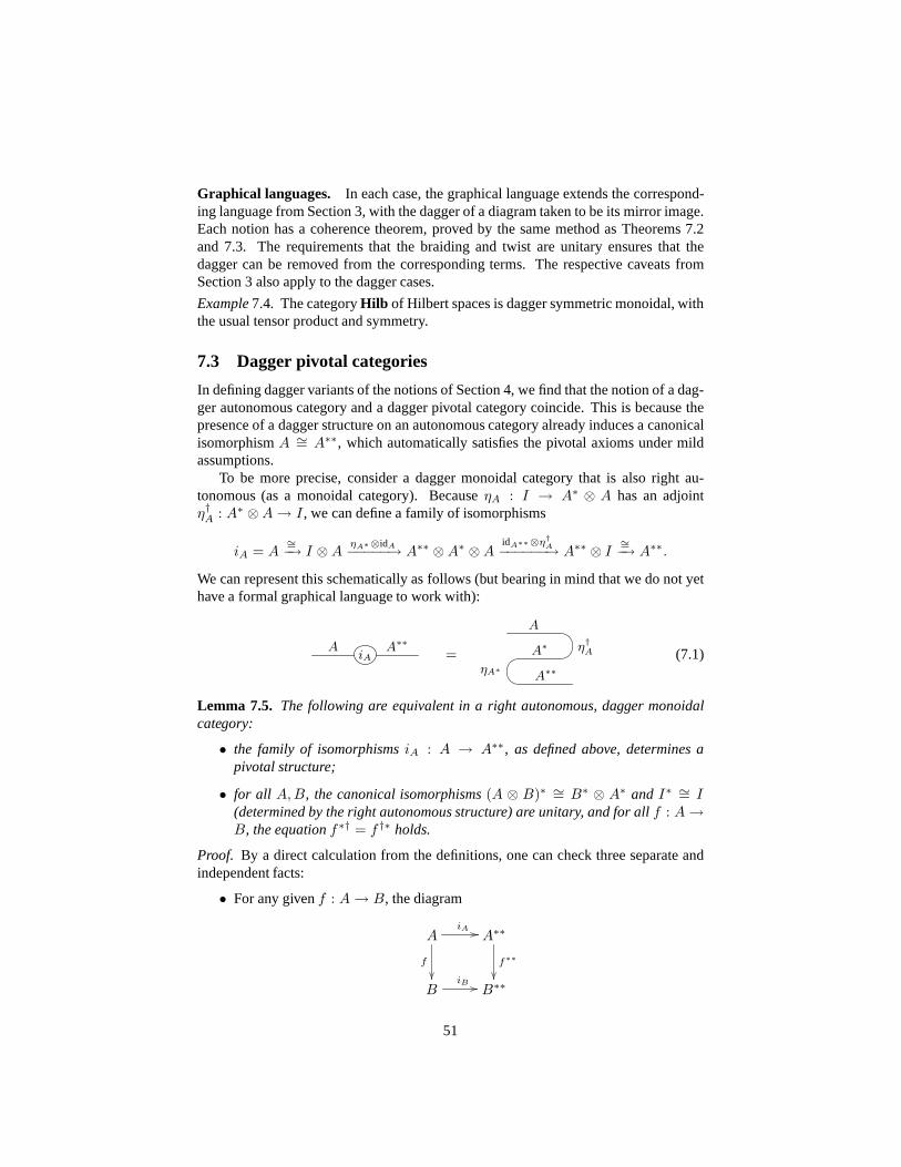
Graphical languages. In each case, the graphical language extends the correspond-ing language from Section 3, with the dagger of a diagram taken to be its mirror image.Each notion has a coherence theorem, proved by the same method as Theorems 7.2and 7.3. The requirements that the braiding and twist are unitary ensures that thedagger can be removed from the corresponding terms. The respective caveats fromSection 3 also apply to the dagger cases.

Example7.4. The categoryHilb of Hilbert spaces is dagger symmetric monoidal, withthe usual tensor product and symmetry.

7.3 Dagger pivotal categories

In defining dagger variants of the notions of Section 4, we findthat the notion of a dag-ger autonomous category and a dagger pivotal category coincide. This is because thepresence of a dagger structure on an autonomous category already induces a canonicalisomorphismA ∼= A∗∗, which automatically satisfies the pivotal axioms under mildassumptions.

To be more precise, consider a dagger monoidal category thatis also right au-tonomous (as a monoidal category). BecauseηA : I → A∗ ⊗ A has an adjointη†A : A∗ ⊗ A → I, we can define a family of isomorphisms

iA = A∼=−→ I ⊗ A

ηA∗⊗idA−−−−−→ A∗∗ ⊗ A∗ ⊗ A

idA∗∗⊗η†A−−−−−−→ A∗∗ ⊗ I

∼=−→ A∗∗.

We can represent this schematically as follows (but bearingin mind that we do not yethave a formal graphical language to work with):

AiA

A∗∗

=

A

η†AA∗

ηA∗A∗∗

(7.1)

Lemma 7.5. The following are equivalent in a right autonomous, dagger monoidalcategory:

• the family of isomorphismsiA : A → A∗∗, as defined above, determines apivotal structure;

• for all A, B, the canonical isomorphisms(A ⊗ B)∗ ∼= B∗ ⊗ A∗ and I∗ ∼= I

(determined by the right autonomous structure) are unitary, and for allf : A →B, the equationf∗† = f †∗ holds.

Proof. By a direct calculation from the definitions, one can check three separate andindependent facts:

• For any givenf : A → B, the diagram

AiA

f

A∗∗

f∗∗

BiB

B∗∗

51

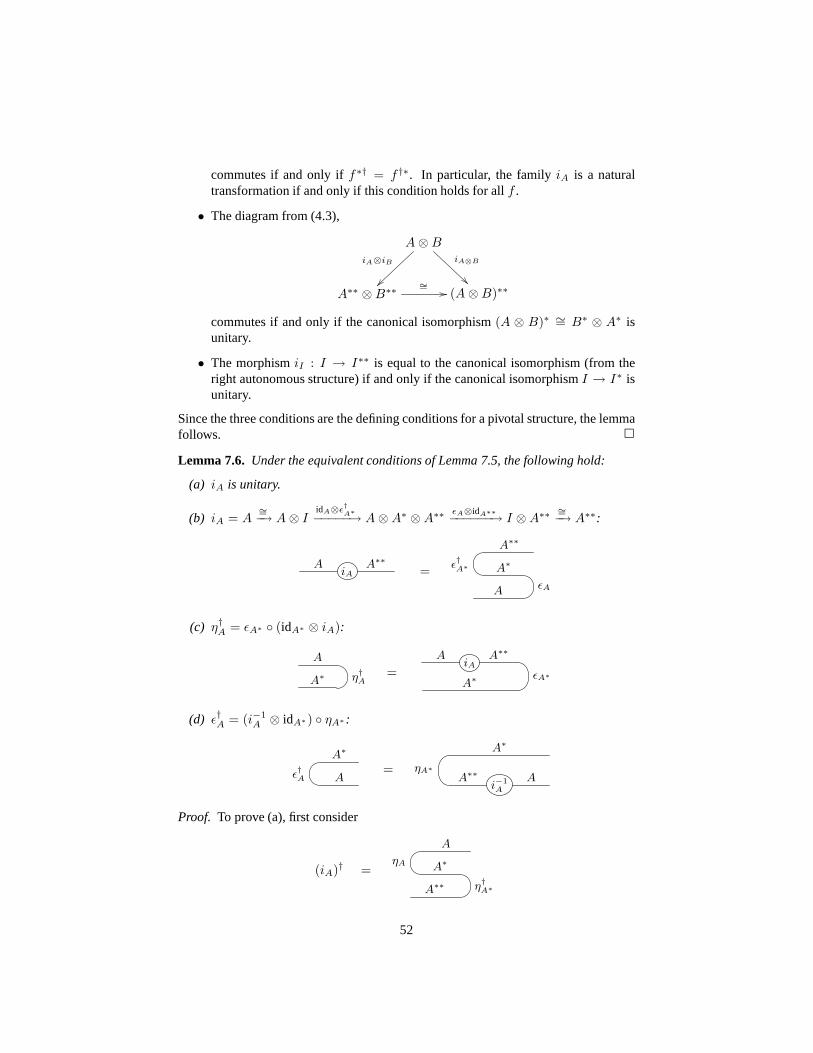
commutes if and only iff∗† = f †∗. In particular, the familyiA is a naturaltransformation if and only if this condition holds for allf .

• The diagram from (4.3),

A ⊗ B

iA⊗iB iA⊗B

A∗∗ ⊗ B∗∗∼=

(A ⊗ B)∗∗

commutes if and only if the canonical isomorphism(A ⊗ B)∗ ∼= B∗ ⊗ A∗ isunitary.

• The morphismiI : I → I∗∗ is equal to the canonical isomorphism (from theright autonomous structure) if and only if the canonical isomorphismI → I∗ isunitary.

Since the three conditions are the defining conditions for a pivotal structure, the lemmafollows. 2

Lemma 7.6. Under the equivalent conditions of Lemma 7.5, the followinghold:

(a) iA is unitary.

(b) iA = A∼=−→ A ⊗ I

idA⊗ǫ†A∗

−−−−−→ A ⊗ A∗ ⊗ A∗∗ ǫA⊗idA∗∗−−−−−−→ I ⊗ A∗∗

∼=−→ A∗∗:

AiA

A∗∗

=ǫ†A∗

A∗∗

A∗

AǫA

(c) η†A = ǫA∗ ◦ (idA∗ ⊗ iA):

A

η†AA∗ =

AiA

A∗∗

ǫA∗A∗

(d) ǫ†A = (i−1

A ⊗ idA∗) ◦ ηA∗ :

ǫ†A

A∗

A= ηA∗

A∗

A∗∗

i−1

A

A

Proof. To prove (a), first consider

(iA)† =ηA

A

A∗

A∗∗ η†A∗

52

By definition of adjoint mates, we have

(iA)†∗ =

A∗

η†A∗A∗∗

ηA∗∗A∗∗∗

But this is just the definition ofiA∗ , therefore(iA)†∗ = iA∗ . By definition,iA is unitaryiff (iA)† = i−1

A , iff (iA)†∗ = (i−1A )∗, iff iA∗ = (i−1

A )∗ = (i∗A)−1. Sincei is a monoidalnatural transformation, this holds by Saavedra Rivano’s Lemma (Lemma 4.9).

To prove (b), note that the right-hand side is the inverse of(iA)†. Therefore, (b) isequivalent to (a).

Finally, equations (c) and (d) are restatements of the definition of iA from (7.1).2

Remark7.7. The equivalence between (a) and (b) in Lemma 7.6 holds only ifiA isdefined as in (7.1). It does not hold for an arbitrary pivotal structure on a right au-tonomous dagger monoidal category.

Armed with these results, we finally state the two equivalentdefinitions of a daggerpivotal category:

Definition. A dagger pivotal categoryis defined in one of the following equivalentways:

1. as a dagger monoidal, right autonomous category such thatthe natural isomor-phisms(A⊗B)∗ ∼= B∗ ⊗A∗ andI∗ ∼= I (from the right autonomous structure)are unitary, and such thatf∗† = f †∗ holds for all morphismsf ; or

2. as a pivotal, dagger monoidal category satisfying the condition in Lemma 7.6(c)(or equivalently, (d)).

The first form of this definition is much easier to check in practice. The secondform is more suitable for the proof of the coherence theorem below.

Remark7.8. In a dagger pivotal category, the operation(−)∗ arises from an adjunction(in the categorical sense) ofobjects, with associated unit, counit, and adjoint mates.On the other hand, the operation(−)† arises from an adjunction (in the linear algebrasense) ofmorphisms. The two concepts should not be confused with each other.

Graphical language. The graphical language of dagger pivotal categories is likethatof pivotal categories, where the adjoint of a diagram is given, as usual, by its mirrorimage. For example:

A

g CB

B

†

=g

A

CB

B

53

Note that in the graphical language, adjoint matesf∗ : B∗ → A∗ are represented byrotation and adjointsf † : B → A by mirror image. Therefore, each morphism variablef : A → B induces four kinds of boxes:

f =A

fB

f † =B

fA

f∗† =A

fB

f∗ =B

fA

Also note that, unlike the informal notation used above, thegraphical languagedoes not explicitly display the isomorphismiA : A → A∗∗, and it does not explicitlydistinguishηA : I → A∗ ⊗ A from ǫ

†A∗ : I → A∗ ⊗ A∗∗. This is justified by the

following coherence theorem.

Theorem 7.9(Coherence for dagger pivotal categories). A well-formed equation be-tween morphisms in the language of dagger pivotal categories follows from the axiomsof dagger pivotal categories if and only if it holds in the graphical language up toplanar isotopy, including rotation of boxes (by multiples of 180 degrees).

Proof. This follows from coherence of pivotal categories (Theorem4.14), by the sameargument used in the proof of Theorem 7.3. The equations fromLemma 7.6(c) and(d), and the fact thatiA is unitary, can be used to replaceη

†A, ǫ

†A, andi

†A by equivalent

terms not containing†. 2

7.4 Other dagger pivotal notions

It is possible to define dagger variants of the remaining pivotal notions from Section 4:

Definition. A dagger pivotal category isspherical(respectivelyspacial) if it is spher-ical (respectively spacial) as a pivotal category.

Definition. A dagger braided pivotal categoryis a dagger pivotal category with aunitary braidingcA,B : A ⊗ B → B ⊗ A.

Remark7.10. Like any braided pivotal category, a dagger braided pivotalcategory isbalanced by Lemma 4.20. However, in general the resulting twist θA : A → A is notunitary. In fact,θA is unitary in this situation if and only ifθA∗ = (θA)∗, i.e., if andonly if the category is tortile.

Definition. A dagger tortile categoryis defined in one of the following equivalentways:

1. as a dagger braided pivotal category in which the canonical twist θA, defined asin Lemma 4.20, is unitary;

2. as a tortile, dagger monoidal category such that the braiding is unitary, and suchthatǫA andηA satisfy the (equivalent) conditions of Lemma 7.6(c) and (d); or

54

3. as a dagger balanced monoidal category that is right autonomous and satisfies

θA =

A A

ηA A∗ η†A

(7.2)

The first form of this definition emphasizes the relationshipto dagger pivotal cate-gories. The second form is easiest to check if a category is already known to be tortile.Finally, the third form takesǫA, ηA, cA,B andθA as primitive operations and does notmention the pivotal structureiA at all. The pivotal structure, in this case, is definablefrom (4.7) or (7.1), with the condition (7.2) ensuring that the two definitions coincide.

Definition ([1, 33]). A dagger compact closed categoryis a dagger tortile categorysuch thatθA = idA for all A. Equivalently, it is a dagger symmetric monoidal categorythat is right autonomous and satisfies

ηA

A

A∗ = ǫ†A

A∗ A

A A∗ (7.3)

The equivalence of the two definition is immediate from the third form of the defini-tion of dagger tortile categories. Note that (7.2) is equivalent to (7.3) in the symmetriccase. Further, these conditions are equivalent to the condition in Lemma 7.6(d).

Example7.11. The categoryFdHilb of finite dimensional Hilbert spaces is daggercompact closed, withA∗ the usual dual space of linear functions fromA to I, and withf † the usual linear algebra adjoint.

Graphical languages. Each of the notions defined in this section (except the spher-ical notion) has a graphical language, extending the corresponding graphical languagefrom Section 4, with the dagger of a diagram taken to be its mirror image. Each no-tion has a coherence theorem, proved by the same method as Theorems 7.2 and 7.3.As expected, equivalence of diagrams is up to isomorphism (for spacial dagger piv-otal categories); up to regular isotopy (for dagger braidedpivotal categories); up toframed 3-dimensional isotopy (for dagger tortile categories); and up to isomorphism(for dagger compact closed categories).

7.5 Dagger traced categories

There is no difficulty in defining dagger variants of each of the traced notions of Sec-tion 5. A (left or right) trace on a dagger monoidal category is called adagger traceifit satisfies

(Tr f)† = Tr(f †) (7.4)

For example: adagger right traced categoryis a right traced dagger monoidal categorysatisfying (7.4). A balanced traced category isdagger balanced tracedif it is daggerbalanced and satisfies (7.4). And similarly for the other notions. The representationtheorems of Section 5 extend to these dagger variants:

55

Theorem 7.12(Representation of dagger braided/balanced/symmetric traced categories).Every dagger braided [balanced, symmetric] traced category can be fully and faithfullyembedded in a dagger braided pivotal [dagger tortile, dagger compact closed] cate-gory, via a dagger braided [balanced, symmetric] traced functor. 2

The proof, in each case, is by Joyal, Street, and Verity’s Int-construction [24], whichrespects the dagger structure.

Graphical languages. The graphical language of each class of traced categories ex-tends to the corresponding dagger traced categories, in a way suggested by equation(7.4). As usual, the dagger of a diagram is its mirror image, thus for example

X X

Af

B

†

=X X

Bf

A

The coherence theorems of Section 5 extend to this setting.

7.6 Dagger biproducts

In a dagger category, ifA⊕B is a categorical product (with projectionsπ1 : A⊕B → A

andπ2 : A ⊕ B → B), then it is automatically a coproduct (with injectionsπ†1 : A →

A ⊕ B andπ†2 : B → A ⊕ B). It therefore makes sense to define a notion ofdagger

biproduct.

Definition. A dagger biproduct categoryis a biproduct category carrying a daggerstructure, such thatπ†

i = ιi : Ai → A1 ⊕ A2 for i = 1, 2.

As in Section 6.3, we can equivalently define a dagger biproduct category as adagger symmetric monoidal category, together with naturalfamilies of morphisms

∆A : A → A ⊗ A, 3A : A → I, ∇A : A ⊗ A → A, 2A : I → A,

such that∆†A = ∇A and3

†A = 2A, satisfying the axioms in Table 7.

Graphical language. The graphical language of dagger biproduct categories is likethat of biproduct categories, where the dagger of a diagram is taken to be its mirrorimage. For example,

f g

†

= g f

56

Theorem 7.13(Coherence for dagger biproduct categories). A well-formed equationbetween morphism terms in the language of dagger biproduct categories follows fromthe axioms of dagger biproduct categories if and only if it holds in the graphical lan-guage, up to isomorphism of diagrams, the diagrammatic manipulations shown in Ta-ble 8, and their duals.

Proof. By reduction to biproduct categories, as in the proofs of Theorems 7.2 and 7.3.The axiomsƠ

A = ∇A and3†A = 2A allow † to be removed from anywhere but a

morphism variable. 2

Finally, there is an obvious notion ofdagger traced biproduct category(which isreally a dagger traced dagger biproduct category), with graphical language derivedfrom traced biproduct categories.

8 Bicategories

A bicategory [6] is a generalization of a monoidal category.In addition to objectsA, B, . . . and morphismsf, g, . . ., one now also considers0-cellsα, β, . . ., which wecan visualize ascolors. For example, consider the following diagram. It is a standarddiagram for monoidal categories, except that the areas between the wires have beencolored.

blue

red

green

yellow

f

g

A

F

E

green

D

B

C

As usual, we have objectsA, B, C, D, E, F and morphismsf : A → C ⊗ D andg : B ⊗ C → F ⊗ E. But now there are also 0-cells called green, red, yellow, andblue. In such diagrams, each object has asource, which is the 0-cell just above it, anda target, which is the 0-cell just below it. For example, we haveA : green→ yellow,B : yellow → blue, and so on. It is now clear that, to be consistently colored, suchdiagrams have to satisfy some coloring constraints. The constraints are:

• The tensorB ⊗ A of two objects may only be formed if the target ofA is equalto the source ofB. In symbols, for any 0-cellsα, β, γ, if A : α → β andB : β → γ, thenB ⊗ A : α → γ.

• If f : A → B is a morphism, thenA andB must have a common source and acommon target. In symbols, iff : A → B andA : α → β, thenB : α → β.

• One also requires a unit objectIα : α → α for every colorα.

As an illustration of the second property, considerf : A → C ⊗ D in the aboveexample, whereA : green→ yellow andC ⊗ D : green→ yellow. Subject to theabove coloring constraints, a bicategory is then required to satisfy exactly the same

57

axioms as a monoidal category. Notice, for example, that iff : A → B andg :B → C andf, g are well-colored, then so isg ◦ f : A → C. Also, the identity maps

idA : A → A, the associativity mapαA,B,C : (A⊗B)⊗C∼=−→ A⊗ (B ⊗C), and the

other structural maps are well-colored. In particular, a monoidal category is the samething as a one-object bicategory.

To give a detailed account of bicategories and their graphical languages is beyondthe scope of this paper. We have already discussed over 30 different flavors of monoidalcategories, and the reader can well imagine how many possible variations of bicate-gories there are, with 2-, 3-, and 4-dimensional graphical languages, once one consid-ers bicategorical versions of braids, twists, adjoints, and traces. There are even morevariations if one considers tricategories and beyond. We refer the reader to [6] for thedefinition and basic properties of bicategories, and to [41], [2, Sec. 7] for a taste oftheir graphical languages.

9 Beyond a single tensor product

All the categorical notions that we have considered in this paper have just a singletensor product, which we represented as juxtaposition in the graphical languages. Fornotions of categories with more than one tensor product, thegraphical languages getmuch more complicated. The details are beyond the scope of this paper, so we justoutline the basics and give some references.

Examples of categories with more than one tensor are linearly distributive cate-gories [13] and *-autonomous categories [4]. Both of these notions are models of mul-tiplicative linear logic [17]. These categories have two tensors, often called “tensor”and “par”, and written

A ⊗ B and A#B.

The two tensors are related by some morphisms, such asA⊗(B#C) → (A⊗B)#C,while other similar morphisms, such as(A⊗B)#C → A⊗ (B#C), are not present.

To make a graphical language for more than one tensor product, one must label thewires by morphism terms, rather than morphism variables. One must also introducespecial tensor and par nodes as shown here:

B

⊗A⊗B

A

A⊗B⊗

B

A

B # A#B

A

A#B # B

A

,

along with similar nodes for the units. Equivalence of diagrams must be taken upto axiomatic manipulations, such as the following, which iscalledcut eliminationinlogic:

B

⊗A⊗B

⊗

B

AA

=B

A

.

Finally, one must state acorrectness criterion, to explain why certain diagrams, suchas the left one following, are well-formed, while others, such as the right one, are not

58

well-formed.

A⊗B⊗

B

A

⊗A⊗B A#B # B

A

⊗A⊗B

The resulting theory is called the theory ofproof nets, and was first given by Girardfor unit-free multiplicative linear logic [17]. It was later extended to include the tensorunits by Blute et al. [8].

10 Summary

Table 10 summarizes the graphical languages from Sections 2–6. The name of eachclass of categories is shown along with a typical diagram or equation. The arrowsindicate forgetful functors. We have omitted spherical categories, because they do notpossess a graphical language modulo a natural notion of isotopy.

The letterd indicates the dimension of the diagrams, and the letteri indicates thedimension of the ambient space for isotopy. Ifi > d, then isotopy coincides withisomorphism of diagrams. Special cases are “3f” for framed diagrams and framed iso-topy in 3 dimensions; “2+” for two-dimensional diagram withcrossings (i.e., isotopy istaken on 2-dimensional projections, rather than on 3-dimensional diagrams); “reg” forregular isotopy; and “rot” to indicate that isotopy includes rotation of boxes. Finally,“eqn” indicates that equivalence of diagrams is taken modulo equational axioms.

The letterc indicates the status of a coherence theorem. This is usuallya referenceto a proof of the theorem, or “conj” if the result is conjectured. A checkmark “√” indi-cates a result that is folklore or whose proof is trivial. “int” indicates that the coherencetheorem follows from a version of Joyal, Street, and Verity’s Int-construction, and thecorresponding coherence theorem for pivotal categories. An asterisk “∗” indicates thatthe result has only been proved for simple signatures.

Dagger variants can be defined of all of the notions shown in Table 10, except theplanar autonomous and braided autonomous notions. Finally, bicategories require theirown (presumably much larger) table and are not included here.

59

Progressive Traced Autonomous

Category

d:1 i:1 c:√

Right traced

d:2 i:2 c:conj

Planar autonomous(rigid)

d:2 i:2 c:[21]

Planar monoidal

d:2 i:2 c:[21, 22]

Planar traced

d:2 i:2 c:conj

Planar pivotal(sovereign)

d:2 i:2.rot c:[16]∗

Spacial monoidal

=

d:2 i:3 c:conj

Spacial traced

=

d:2 i:3 c:conj

Spacial pivotal

=

d:2 i:3 c:conj

Braided autonomous

d:2+ i:reg c:[16]∗

Braided monoidal

d:3 i:3 c:[22]

Braided traced

d:2+ i:reg.rot c:int∗

Braided pivotal(balanced autonomous)

d:2+ i:reg.rotc:[16]∗

Balanced monoidal

d:3f i:3f c:[22]

Balanced traced

=

=

d:3f i:3f c:int∗

Tortile (ribbon)

d:3f i:3f c:[34]∗

Symmetric monoidal

d:3 i:4 c:[22]

Symmetric traced

d:3 i:4 c:int∗

Compact closed

d:3 i:4 c:[27]∗

Product

=

d:3 i:eqn c:√

Traced product

d:3 i:eqn c:√

Coproduct

=

d:3 i:eqn c:√

Traced coproduct

d:3 i:eqn c:√

Biproduct

=

d:3 i:eqn c:√

Traced biproduct

d:3 i:eqn c:√

Table 10: Summary of monoidal notions and their graphical languages

60

References

[1] S. Abramsky and B. Coecke. A categorical semantics of quantum protocols. InProceedings of the 19th Annual IEEE Symposium on Logic in Computer Science,LICS 2004, pages 415–425. IEEE Computer Society Press, 2004.

[2] J. C. Baez and J. Dolan. Higher-dimensional algebra and topological quantumfield theory.Journal of Mathematical Physics, 36(11):6073–6105, 1995.

[3] E. S. Bainbridge. Feedback and generalized logic.Information and Control,31:75–96, 1976.

[4] M. Barr. *-Autonomous Categories. Lectures Notes in Mathematics 752.Springer, 1979.

[5] J. W. Barrett and B. W. Westbury. Spherical categories.Advances in Mathematics,143:357–375, 1999.

[6] J. Benabou. Introduction to bicategories, part I. InReports of the Midwest Cate-gory Seminar, Lecture Notes in Mathematics 47, pages 1–77. Springer, 1967.

[7] S. L. Bloom and Z.Esik. Axiomatizing schemes and their behaviors.Journal ofComputer and System Sciences, 31:375–393, 1985.

[8] R. F. Blute, J. R. B. Cockett, R. A. G. Seely, and T. H. Trimble. Natural deductionand coherence for weakly distributive categories.Journal of Pure and AppliedAlgebra, 113(3):229–296, 1996.

[9] V.-E. Cazanescu. On context-free trees.Theoretical Comput. Sci., 41:33–50,1985.

[10] V.-E. Cazanescu and G. Stefanescu. Towards a new algebraic foundation offlowchart scheme theory.Fundamenta Informaticae, 13:171–210, 1990. Alsoappeared as: INCREST Preprint Series in Mathematics 43, Bucharest, 1987.

[11] V.-E. Cazanescu and G. Stefanescu. Feedback, iteration and repetition. InG. Paun, editor,Mathematical aspects of natural and formal languages, pages43–62. World Scientific, Singapore, 1995. Also appeared as:INCREST PreprintSeries in Mathematics 42, Bucharest, 1988.

[12] V.-E. Cazanescu and C. Ungureanu. Again on advice on structuring compilers andproving them correct. Preprint Series in Mathematics 75, INCREST, Bucharest,1982.

[13] J. R. B. Cockett and R. A. G. Seely. Weakly distributive categories.Pure andApplied Algebra, 114(2):133–173, 1997.

[14] Z. Esik. Identities in iterative and rational algebraic theories. ComputationalLinguistics and Computer Languages, XIV:183–207, 1980.

61

[15] P. J. Freyd and D. N. Yetter. Braided compact closed categories with applicationsto low dimensional topology.Advances in Mathematics, 77:156–182, 1989.

[16] P. J. Freyd and D. N. Yetter. Coherence theorems via knottheory.Journal of Pureand Applied Algebra, 78:49–76, 1992.

[17] J.-Y. Girard. Linear logic.Theoretical Comput. Sci., 50:1–102, 1987.

[18] M. Hasegawa.Models of Sharing Graphs: A Categorical Semantics of let andletrec. PhD thesis, Department of Computer Science, University ofEdinburgh,July 1997.

[19] A. Joyal and R. Street. The geometry of tensor calculus II. Unpublished draft,available from Ross Street’s website.

[20] A. Joyal and R. Street. Braided monoidal categories. Mathematics Report860081, Macquarie University, Nov. 1986.

[21] A. Joyal and R. Street. Planar diagrams and tensor algebra. Unpublishedmanuscript, available from Ross Street’s website, Sept. 1988.

[22] A. Joyal and R. Street. The geometry of tensor calculus I. Advances in Mathe-matics, 88(1):55–112, 1991.

[23] A. Joyal and R. Street. Braided tensor categories.Advances in Mathematics,102:20–78, 1993.

[24] A. Joyal, R. Street, and D. Verity. Traced monoidal categories. MathematicalProceedings of the Cambridge Philosophical Society, 119:447–468, 1996.

[25] L. H. Kauffman. An invariant of regular isotopy.Transactions of the AmericanMathematical Society, 318(2):417–471, 1990.

[26] G. M. Kelly. An abstract approach to coherence. In S. MacLane, editor,Coher-ence in Categories, Lecture Notes in Mathematics 281, pages 106–147. Springer,1972.

[27] G. M. Kelly and M. L. Laplaza. Coherence for compact closed categories.Journalof Pure and Applied Algebra, 19:193–213, 1980.

[28] S. Mac Lane. Natural associativity and commutativity.Rice University Studies,49:28–46, 1963.

[29] S. Mac Lane. Categories for the Working Mathematician. Graduate Texts inMathematics 5. Springer, 1971.

[30] R. Penrose. Applications of negative dimensional tensors. In D. J. A. Welsh, edi-tor, Combinatorial Mathematics and its Applications, pages 221–244. AcademicPress, New York, 1971.

[31] K. Reidemeister.Knotentheorie. Springer, Berlin, 1932; Chelsea, New York,1948. English translation:Knot Theory, BCS Associates, 1983.

62

[32] N. Saavedra Rivano.Categories Tanakiennes. Lecture Notes in Mathematics 265.Springer, 1972.

[33] P. Selinger. Dagger compact closed categories and completely positive maps. InProceedings of the 3rd International Workshop on Quantum Programming Lan-guages, Electronic Notes in Theoretical Computer Science 170, pages 139–163.Elsevier Science, 2007.

[34] M. C. Shum. Tortile tensor categories.Journal of Pure and Applied Algebra,93:57–110, 1994.

[35] G. Stefanescu. An algebraic theory of flowchart schemes. InProceedings ofthe 11th Colloquium on Trees in Algebra and Programming, CAAP’86, LectureNotes in Computer Science 214, pages 60–73. Springer, 1986.

[36] G. Stefanescu. On flowchart theories, part I. the deterministic case.Journal ofComputer and System Sciences, 35(2):163–191, 1987.

[37] G. Stefanescu. On flowchart theories: Part II. the nondeterministic case.tcs,52:307–340, 1987.

[38] G. Stefanescu. Feedback theories (a calculus for isomorphism classes of flowchartschemes).Revue Roumaine de Mathematiques Pures et Appliquees, 35:73–79,1990. Also appeared as: INCREST Preprint Series in Mathematics 24, Bucharest,1986.

[39] G. Stefanescu. Algebra of flownomials. Technical Report TUM-I9437, Technis-che Univeritat Munchen, 1994.

[40] G. Stefanescu.Network Algebra. Springer, 2000.

[41] R. Street. Low-dimensional topology and higher-ordercategories. InProceedingsof the International Category Theory Conference (CT’95), 1995. Available fromhttp://www.mta.ca/∼cat-dist/ct95.html.

[42] V. G. Turaev.Quantum Invariants of Knots and 3-Manifolds. Studies in Mathe-matics 18. Walter De Gruyter & Co., Berlin, 1994.

[43] D. N. Yetter. Framed tangles and a theorem of Deligne on braided deformationsof tannakian categories. In M. Gerstenhaber and J. D. Stasheff, editors,Defor-mation Theory and Quantum Groups with Applications to Mathematical Physics,Contemporary Mathematics 134, pages 325–349. Americal Mathematical Soci-ety, 1992.

63