causal hazard ratio estimation by instrumental variables ... · pdf filecausal hazard ratio...

Causal Hazard Ratio Estimation By Instrumental Variables or

Principal Stratification

Todd MacKenzie, PhD

Collaborators

• A. James O’Malley

• Tor Tosteson

• Therese Stukel

2

Overview

1. Instrumental variable (I.V.)

2. I.V.s for Hazard Ratio Estimation

3. Principal stratification (P.S.)

4. P.S. for Hazard Ratio Estimation

3

Observational Studies and Confounding

• Confounding is always a threat to observational studies

• Therefore we prefer when possible to conduct

4

Randomized Studies

• Randomized studies yield fair comparisons

• However – Require greater resources

– Tend to be conducted in artificial settings

• Therefore, observational studies deserve more consideration

5

Current Arsenal of Statistical Methods for Overcoming Confounding

1. Adjustment (regression) models

2. Propensity score matching or stratification

3. Inverse propensity weighted – marginal structural models

Bias is removed only to the extent that confounders are included in the model

6

Confounding that cannot be removed

• Goes by different names

– Omitted covariates

– Unmeasured confounders

– Residual confounding

7

Instrumental Variables

• Estimation by I.V can yield unbiased estimates without observing all confounders

8

Instrumental Variables for the Linear Model

• Idea is accessible to any student of an introductory mathematical statistics class

9

Instrumental Variables for the Linear Model

1. Y = a + bX + ε such that Cov(I.V., ε)=0

2. Cov(Y,W) = Cov(a+bX+ε, I.V.) = bCov(X, I.V.)

3. Therefore b = Cov(Y, I.V.) / Cov(X, I.V.)

10

Assumptions

1. Nonzero association of X and the I.V. – Usual rule of thumb: F-test of I.V. and X exceeds 10

11

Assumptions

2. The effect of the I.V. on the Y is strictly through the effect of the I.V on X:

a. There is no direct effect of the I.V. on Y

b. There is no intermediate variable for the effect of the I.V on Y except X: Exclusion Criteria or Absence of Indirect Effect

c. There are no variables that effect both I.V. and Y: No I.V.-Outcome Confounders or Randomization

12

IV X Y

13

IV X Y

There are no paths between IV and Y except through X

14

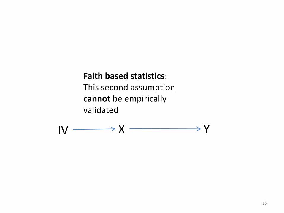
IV X Y

Faith based statistics: This second assumption cannot be empirically validated

15

Other Assumptions Not Necessarily Worth Mentioning

• SUTVA: Stable Unit Treatment Value Assumption – My treatment does not effect your outcome

• Monotonicity

16

Do instrumental variables exist?

• Yes, “man-made” instruments exist:

Randomized Studies – Randomization is an instrument for the effect of

treatment on an endpoint

– The arm a subject is randomized to should have no effect on the endpoint through its effects on the treatment received

17

Do instrumental variables exist in the “real” world?

• Happenstance

• Be on the lookout for natural experiments

• Commonly employed instrumental variables: – Geographic variables (regional rates, distances)

– Care provider propensity to prescribe a treatment

– Calendar time • Before after a health policy change

– See “regression discontinuity”

18

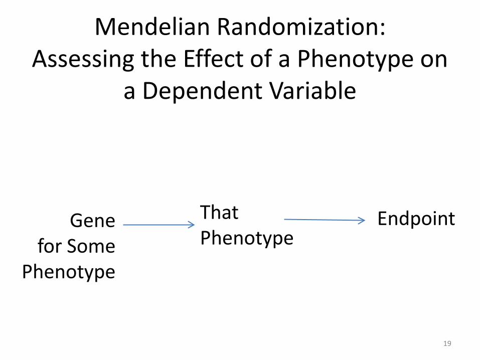
Gene for Some

Phenotype

That Phenotype

Endpoint

Mendelian Randomization: Assessing the Effect of a Phenotype on

a Dependent Variable

19

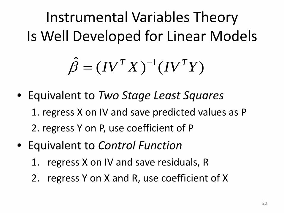
Instrumental Variables Theory Is Well Developed for Linear Models

• Equivalent to Two Stage Least Squares 1. regress X on IV and save predicted values as P

2. regress Y on P, use coefficient of P

• Equivalent to Control Function 1. regress X on IV and save residuals, R

2. regress Y on X and R, use coefficient of X

)()(ˆ 1 YIVXIV TT −=β

20

Our Aim

• To develop an estimator of the hazard ratio using an instrumental variable

21

Challenges

• Non-linear parameterization (e.g., Cox model)

• Right censoring

22

Prior Work in the Literature

• Some in econometrics literature

• Stukel et al (2007) JAMA

23

Original Motivation

Stukel et al “Analysis of Observational Studies in the Presence of Treatment Selection Bias: Effects of Invasive Cardiac Management on AMI Survival Using Propensity Score and Instrumental Variable Methods” JAMA (2007)

24

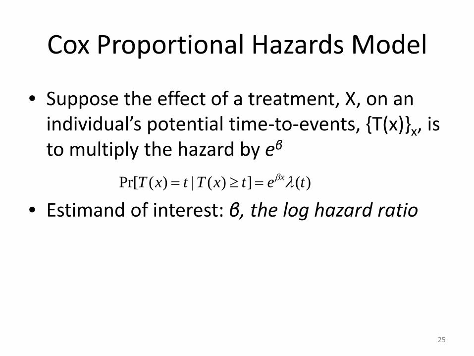
Cox Proportional Hazards Model

• Suppose the effect of a treatment, X, on an individual’s potential time-to-events, {T(x)}x, is to multiply the hazard by eβ

• Estimand of interest: β, the log hazard ratio

)(])(|)(Pr[ tetxTtxT xλβ=≥=

25

Non-Collapsibility of Cox’s Model

• Like most non-linear models (e.g. logistic regression) Cox’s model is not collapsible

• That is, if the conditional distribution of time-to-event T given Z1 and Z2 is a Cox model then the marginal conditional distribution of T given Z1 (obtained by integrating over Z2) is not a Cox model unless Z1 is independent of T

26

A model that collapses to Cox

• The model

for the joint effect of X and Z (e.g., an omitted covariate) , collapses to (integrates out to)

under certain conditions

)(])(|)(Pr[ tetxTtxT xλβ=≥=

ztezZtxTtxT x θλβ +==≥= )(],)(|)(Pr[

27

Incorporating the I.V.

Assuming that the I.V. is independent of the omitted covariate, Z, an argument using risk sets or martingales, e.g.,

can be made that results in the estimating equation on the next slide

0)}]()({..[ ≈−• tetdNVIE xλβ

28

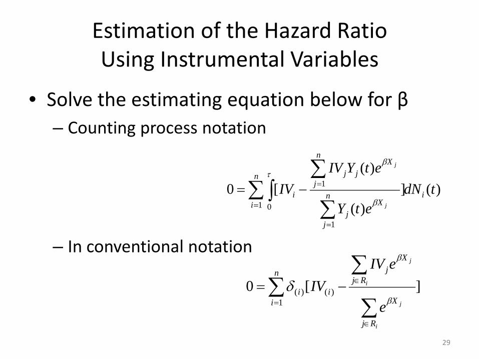
Estimation of the Hazard Ratio Using Instrumental Variables

• Solve the estimating equation below for β – Counting process notation

– In conventional notation

)(])(

)([0

1 0

1

1 tdNetY

etYIVIV i

n

in

j

Xj

n

j

Xjj

ij

j

∑∫∑

∑=

=

=−=τ

β

β

][01

)()(∑∑

∑=

∈

∈−=n

i

Rj

X

Rj

Xj

ii

i

j

i

j

e

eIVIV

β

β

δ

29

Simulations

• Conducted simulations to evaluate bias

• For the unmeasured confounder two models were assume 1. Additive effect of the confounder on the hazard

2. Multiplicative effect (Cox) of the confounder on the hazard

30

Simulation Results for Multiplicative Omitted Covariate

31

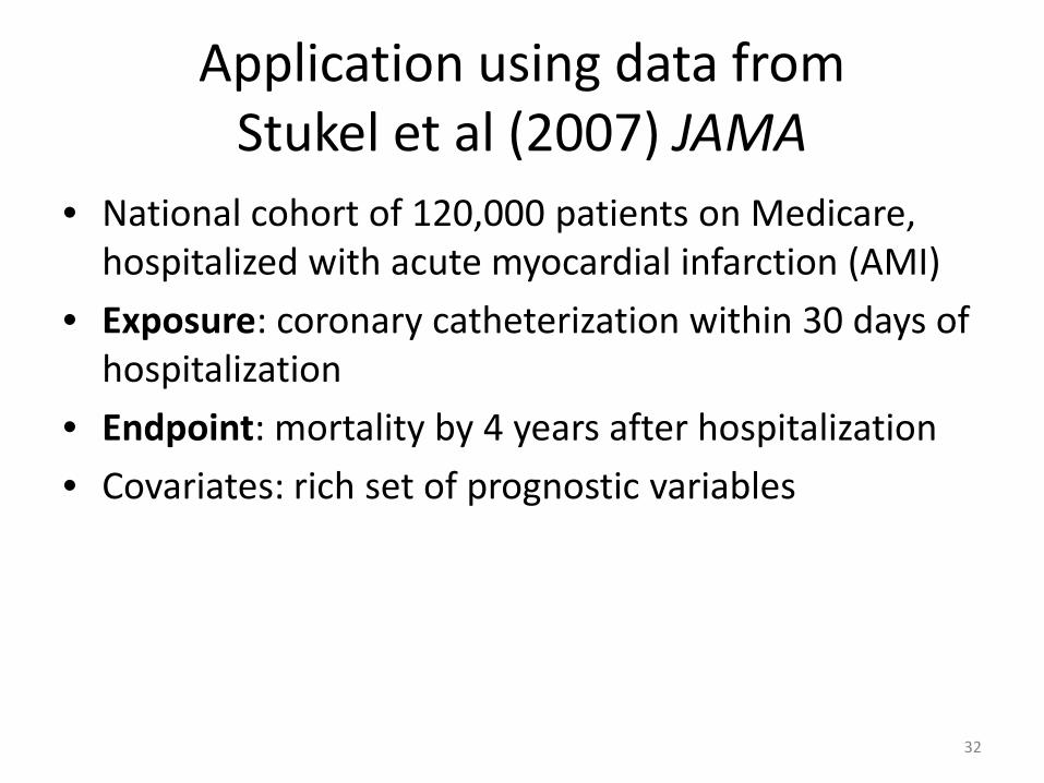
Application using data from Stukel et al (2007) JAMA

• National cohort of 120,000 patients on Medicare, hospitalized with acute myocardial infarction (AMI)

• Exposure: coronary catheterization within 30 days of hospitalization

• Endpoint: mortality by 4 years after hospitalization

• Covariates: rich set of prognostic variables

32

Aim of Stukel’s study

• Estimate the effect of coronary catheterization on survival using three different approaches – Regression (Cox’s model)

– Propensity Scores (with and without matching)

– Instrumental variables

• Compare the estimates to those obtained in randomized studies

33

Instrumental Variables in Stukel et al (2007)

• Instrument: regional cardiac catheterization rate – proportion of eligible patients receiving cardiac catheterization

within 30 days of admission in each area – 566 areas – Assumption: the effect of this proportion on survival is strictly

through its association with an individual’s propensity to have a card. cath.

• Methods for linear instrument variable models applied to survival – Used endpoint of survival at 1 year (4 years) – Excludes subjects who were censored before that time – Converted coefficient from linear model into hazard ratio

34

Example: Effect of coronary catheterization on survival

Approach Hazard Ratio (95%CI) Cox adjusted 0.51 0.50 0.52 Cox adjusted excluding .rst 31 days 0.55 0.54 0.56 Prop Score matched within .05 0.54 0.52 0.56 Stukel L.M. Instrumental Variable at 1 Yr 0.86 0.78 0.94 Stukel L.M. Instrumental Variable at 4 Yrs 0.84 0.79 0.90 Instrumental Variable Estimator (Overall) 0.70 0.60 0.82 Based on First Year 0.72 0.56 0.84

• Whereas randomized studies yielded estimates of 0.80 to 0.92

35

Related Work

• Accelerated Failure Time model

• Additive Hazards Model (Jason Fine)

• Mitra & Small, Chan & Small

• Tchetgen Tchetgen

36

Principal Stratification

Randomized Trial

• Goal: Estimate treatment effect – e.g., drug vs placebo

38

Compliance

• Not all participants comply

39

Common Estimators from a Randomized Trial

• Intention-to-treat

• As treated

• Per protocol

40

Intention-to-treat

• Analyze as randomized

• Unbiased estimate of treatment assignment

• It does not estimate the effect of treatment, were a subject to comply

41

As Treated

• Selection bias is introduced – Treatment is selected as opposed to randomized

42

Per Protocol

• Excludes subjects who did not comply

• What is it estimating ?

43

How to Estimate the effect of treatment?

• What is the effect of treatment, if someone complies with treatment

• Principal Stratification is a framework for defining a meaningful estimand

• To start with, consider the relationship of the exposure a subject receives to the arm of the study they are randomized to

44

Mappings from Support of the Binary Assignment to the Support of the Binary Expsosure ?

• There are 4 mappings from the two possible values of the assignment, R, to the two possible values of the exposure, X

Mapping R to X Principal Strata Name

Identity 0 to 0, 1 to 1 Compliers

Contant Zero

0 to 0, 1 to 0 Never Takers

Constant Unity

0 to 1, 1 to 1 Always Takers

Reverse 0 to 1, 1 to 0 Defiers

45

The Principal Strata

• Latent – Not directly observable

• Names are suggestive but should not be taken at face value

46

No Defiers

• It appears reasonable to assume that there is no defiers (or at least they are very rare)

• Furthermore this assumption facilitates identification of some of the latent strata

• This assumption is called Monotonicity

47

Identification of Strata from the Observations

Assignment Exposure Principal Strata

0 0 Complier (Co) or Never Taker (NT)

0 1 Always Taker (AT)

1 0 Never Taker (NT)

1 1 Complier (Co) or Always Taker (AT)

48

Complier Average Causal Effect for Continuous Endpoints

50

Extending Principal Stratification to Non-Linear Parameter Estimation

• The following slides show a way of arriving at estimates of the distributions of an endpoint in treated compliers and in untreated compliers

• These respective distributions can then be used to estimate parameters that characterize these distributions

51

Arithmetic Shows The Potential Outcomes in the Compliers Can be Identified Using the

Observable Distributions

Potential Outcomes in the Compliers

Mixture of Weights

Y(0)|PS=Co Y(X)|R=0,X=0 and Y(X)|PS=NT (1+pNT/pC0 , -pNT/pCo)

Y(1)|PS=Co Y(X)|R=1,X=1 and Y(X)|PS=AT (1+pCo/pAT , -pAT/pCo)

53

Operationalizing: Weights

• To estimate the distribution, or parameters related to the distribution of the potential outcomes on the compliers, use the observeable samples but weight them in proportion to the weights on the previous slide

• Note: Some of the weights are negative ! – Negative weights not readily implemented with

some software (e.g. R)

54

Principal Stratification Weights for Hazard Ratio Estimation

• To estimate the hazard ratio of Cox’s model we apply weights to the observed follow-up and censoring indicators to create samples from treated and untreated individuals from the complier strata

55

Results of Simulations

56

Summary

• It is possible to estimate the causal hazard ratio with little or no bias in the setting of all-or-nothing compliance

• I.T.T., Per Protocol and As Treated Estimators are Biased

57

Future Steps

• Instrumental Variables – Time-varying exposure – e.g. compliance that

varies with time

– Weak instruments

• Principal Stratification – Smooth weights to remove negative values

– Generalization of three principal strata (NT, Co, AT) to a latent variable that is continuous variable indicating propensity for obtaining treatment

58

Causal Inference Syntax

• Exposure X: 1=treatment, 0=no treatment

• Potential outcomes – Y(0) is outcome if there is no treatment

– Y(1) is outcome if there is treatment

• We observe only one of the potential outcomes, Y(X) – The others are counterfactuals

61

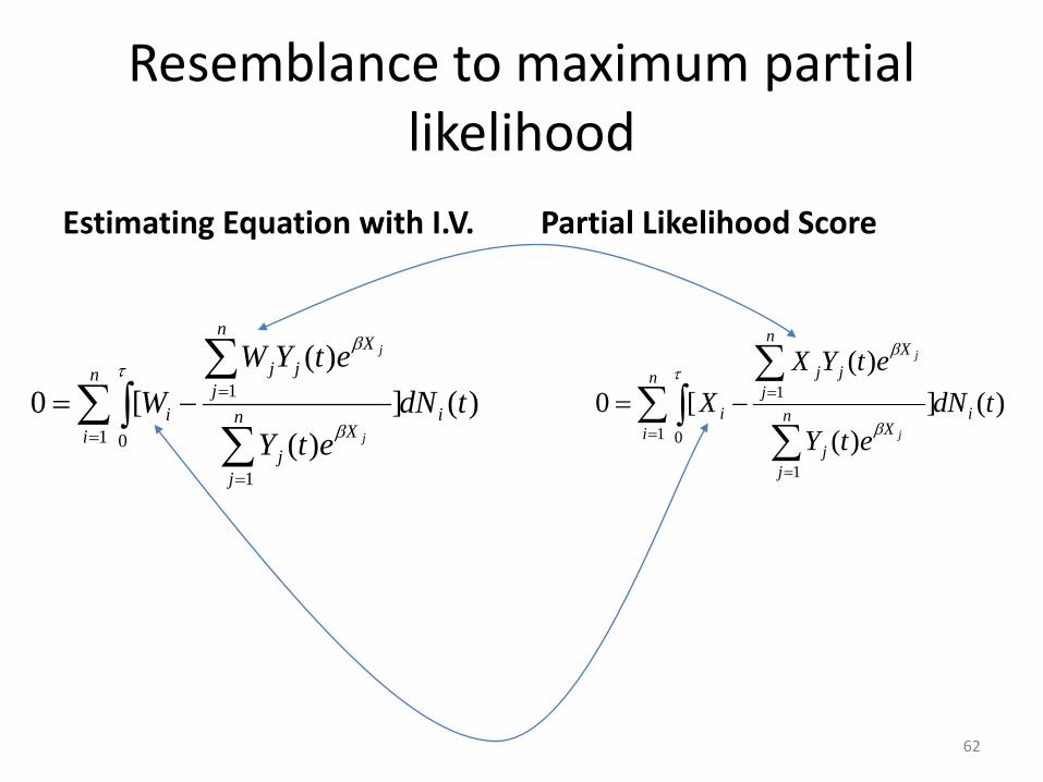
Resemblance to maximum partial likelihood

Estimating Equation with I.V.

)(])(

)([0

1 0

1

1 tdNetY

etYWW i

n

in

j

Xj

n

j

Xjj

ij

j

∑∫∑

∑=

=

=−=τ

β

β

Partial Likelihood Score

)(])(

)([0

1 0

1

1 tdNetY

etYXX i

n

in

j

Xj

n

j

Xjj

ij

j

∑∫∑

∑=

=

=−=τ

β

β

62

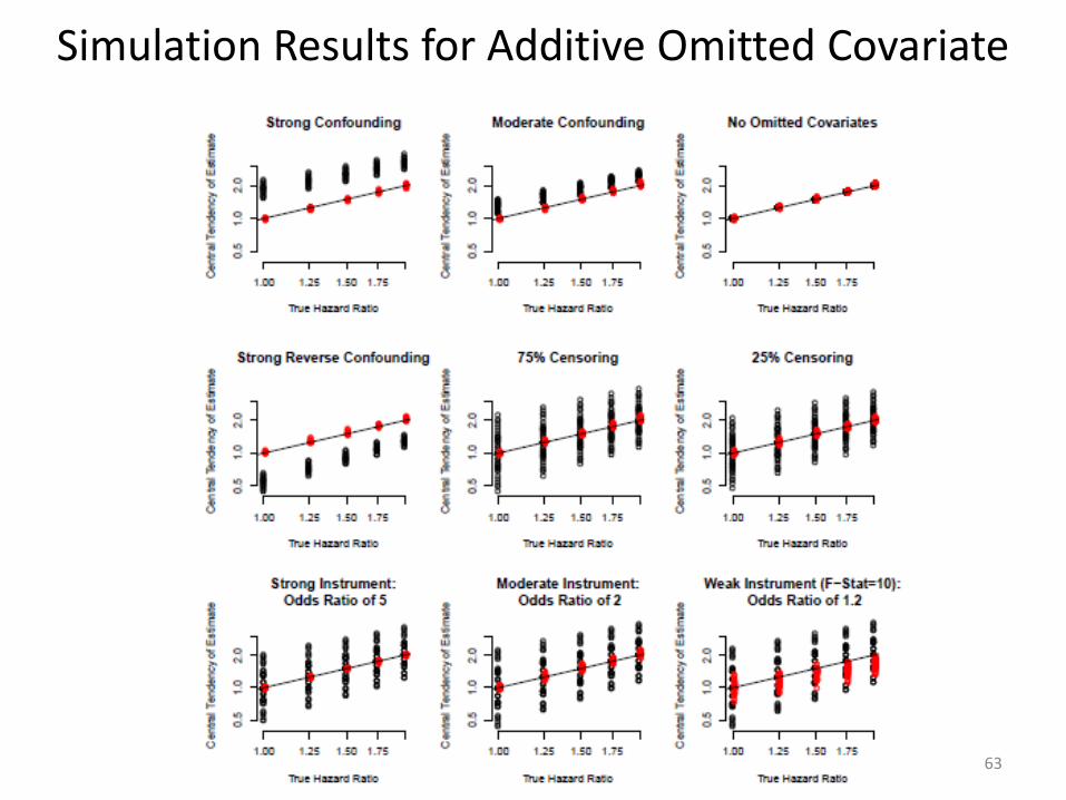
Simulation Results for Additive Omitted Covariate

63

Principal Stratification: When treatment is not accessible to controls • Two classes

• “One sided compliance”

1. Compliers: do as assigned

2. Never takers: will not do treatment regardless of assignment

64

causal hazard ratio estimation by instrumental variables ... · pdf filecausal hazard ratio...

Documents