ccs optima+ stil – ccs optima – operation and maintenance manual ccs-102-p1 rev. s page 6 out of...
TRANSCRIPT

STIL SAS 595, rue Pierre Berthier – Domaine de Saint Hilaire – 13855 Aix-en-Provence cedex 3, France
Tel: +33 (0)4 42 39 66 51 – Fax : +33 (0)4 42 24 38 05 Email : [email protected] – Web site : www.stilsa.com
CCS OPTIMA+
Operating and maintenance manual

STIL – CCS Optima – Operation and maintenance manual CCS-102-P1 Rev. S
Page 2 out of 85
SUMMARY
PART I: INTRODUCTION
1 PRESENTATION OF THE THE CCS OPTIMA AND THE CCS OPTIMA+ ...................................... 6
1.1 CONTROLLER ........................................................................................................................................... 6 1.1.1 Description ...................................................................................................................................... 6 1.1.2 LED indicators ................................................................................................................................ 7
1.2 OPTICAL PEN AND FIBER OPTICS ............................................................................................................... 7 1.3 THE LIGHT SOURCE .................................................................................................................................. 8 1.4 OPTIONAL ACCESSORIES .......................................................................................................................... 8
1.4.1 Metrology standards ....................................................................................................................... 8
2 SAFETY ......................................................................................................................................................... 9
2.1 ELECTRICAL HAZARDS ............................................................................................................................. 9 2.2 OPTICAL HAZARDS ................................................................................................................................... 9 2.3 GENERAL RECOMMENDATIONS ................................................................................................................ 9 2.4 COMPLIANCE WITH THE EC REGULATION 89/336/EEC « ELECTROMAGNETIC COMPATIBILITY »............ 9 2.5 COMPLIANCE WITH THE ROHS REGULATION ........................................................................................... 9
3 INSTALLATION AND STARTUP ........................................................................................................... 10
3.1 ELECTRICAL CONNECTIONS ................................................................................................................... 10 3.1.1 Power ............................................................................................................................................ 10 3.1.2 RS232 – RS422 connector ............................................................................................................. 10 3.1.3 USB connector .............................................................................................................................. 11 3.1.4 Analog outputs .............................................................................................................................. 11 3.1.5 Synchronization signals................................................................................................................. 11 3.1.6 Encoder connector ........................................................................................................................ 11
3.2 FIBER OPTICS CONNECTIONS .................................................................................................................. 11 3.3 INSTALLING THE USB DRIVER, THE DLL AND THE “CCS MANAGER” SOFTWARE ................................. 12
3.3.1 Installing the USB driver: ............................................................................................................. 12 3.3.2 Installing the software ................................................................................................................... 14
3.4 SENSOR STARTUP ................................................................................................................................... 14
4 BASIC CHARACTERISTICS ................................................................................................................... 15
4.1 CHROMATIC CONFOCAL IMAGING (CCI) ............................................................................................... 15 4.2 APPLICATIONS ....................................................................................................................................... 16 4.3 MEASURING MODES ............................................................................................................................... 16
4.3.1 “Distance” measuring mode ......................................................................................................... 17 4.3.2 “Thickness” measuring mode ....................................................................................................... 17
4.4 MEASURED DATA ................................................................................................................................... 17 4.4.1 The distance data .......................................................................................................................... 17 4.4.2 The Intensity data .......................................................................................................................... 18 4.4.3 Altitude images and Intensity images ............................................................................................ 19
4.5 EXTERNAL SCANNING ............................................................................................................................ 19
5 COMMUNICATION WITH THE CCS OPTIMA .................................................................................. 21

STIL – CCS Optima – Operation and maintenance manual CCS-102-P1 Rev. S
Page 3 out of 85
6 GETTING STARTED (TUTORIAL 1) .................................................................................................... 22
6.1 CONNECTING TO THE CCS OPTIMA ........................................................................................................ 22 6.2 CONFIGURING THE SENSOR .................................................................................................................... 23 6.3 SAVING THE CONFIGURATION ................................................................................................................ 24 6.4 SELECTING THE OUTPUT DATA ............................................................................................................... 25 6.5 VIEWING AND SAVING THE MEASURED DATA ......................................................................................... 26 6.6 ACQUIRING THE DARK SIGNAL .............................................................................................................. 28
6.6.1 Related topics ................................................................................................................................ 28 6.7 ADJUSTING THE LED BRIGHTNESS ......................................................................................................... 29
6.7.1 Minimal brightness level ............................................................................................................... 29 6.8 PLACING THE SAMPLE WITHIN THE MEASUREMENT RANGE OF THE OPTICAL PEN ................................... 29 6.9 ADJUSTING THE SAMPLING RATE ........................................................................................................... 30
7 GOING FURTHER (TUTORIAL 2) ......................................................................................................... 32
7.1 SYNCHRONIZING THE SENSOR WITH OTHER DEVICES ............................................................................. 32 7.1.1 The “Start” trigger mode .............................................................................................................. 32 7.1.2 Training ......................................................................................................................................... 33
7.2 LEARNING MORE ABOUT THE “CCS MANAGER” SOFTWARE .................................................................. 34 7.2.1 Help utility ..................................................................................................................................... 34 7.2.2 Command Terminal ....................................................................................................................... 34 7.2.3 Tools Menu .................................................................................................................................... 35 7.2.4 Preferences Menu .......................................................................................................................... 35
7.3 COMMUNICATING WITH THE CCS OPTIMA BY THE SERIAL LINK ............................................................ 36 7.4 MEASURING THICKNESS ......................................................................................................................... 37
7.4.1 Thickness calibration (refractive index file generation) ............................................................... 37 7.4.2 Minimum measurable thickness .................................................................................................... 37 7.4.3 Maximal measurable thickness ..................................................................................................... 37 7.4.4 Smoothing ...................................................................................................................................... 38 7.4.5 Single surface in “Thickness” mode ............................................................................................. 38 7.4.6 Measuring the Thickness of opaque samples ................................................................................ 38 7.4.7 Training ......................................................................................................................................... 38
PART II: BASIC FEATURES
8 MAIN FUNCTIONS OF THE CCS OPTIMA ......................................................................................... 40
8.1 OPTICAL PEN SELECTION ........................................................................................................................ 40 8.1.1 Optical pen selection ..................................................................................................................... 40 8.1.2 Full scale value of the optical pen currently selected ................................................................... 40 8.1.3 List of optical pens ........................................................................................................................ 40
8.2 DARK SIGNAL......................................................................................................................................... 40 8.2.1 Acquiring and saving the Dark signal ........................................................................................... 41 8.2.2 Getting the minimal rate authorized after Dark acquisition ......................................................... 41 8.2.3 “Fast” Dark .................................................................................................................................. 41
8.3 SAMPLING RATE ..................................................................................................................................... 42 8.3.1 Selecting a preset sampling rate ................................................................................................... 42 8.3.2 “Free” sampling rate .................................................................................................................... 42 8.3.3 Exposure time ................................................................................................................................ 43
8.4 MEASURING MODES ............................................................................................................................... 44 8.5 REFRACTIVE INDEX ................................................................................................................................ 44
8.5.1 Setting a constant refractive index ................................................................................................ 44 8.5.2 Selecting a Refractive index file .................................................................................................... 44
8.6 ADJUSTMENT OF THE LED BRIGHTNESS ................................................................................................ 45 8.7 AVERAGING ........................................................................................................................................... 45 8.8 HOLDING THE LAST VALID VALUE .......................................................................................................... 46 8.9 DEFINING THE ORIGIN OF THE ENCODER MEASURING RANGE ................................................................. 46 8.10 GETTING THE SERIAL NUMBER AND THE FIRMWARE VERSION ................................................................ 46
STIL – CCS Optima – Operation and maintenance manual CCS-102-P1 Rev. S
Page 4 out of 85
8.11 SAVING THE CURRENT CONFIGURATION ................................................................................................. 46 8.12 RESETTING THE SENSOR ......................................................................................................................... 47
9 DIGITAL OUTPUTS ................................................................................................................................. 48
9.1 SELECTION OF THE DATA TO BE TRANSMITTED ...................................................................................... 48 9.1.1 Available data ............................................................................................................................... 48 9.1.2 Data Selection ............................................................................................................................... 48
9.2 SPECIFIC FEATURES OF THE RS232 / RS422 LINK .................................................................................. 49 9.2.1 Configuring of the COM port of the host computer ...................................................................... 49 9.2.2 Limitation of the amount of data transmissible simultaneously .................................................... 50
9.3 SPECIFIC FEATURES OF THE USB LINK ................................................................................................... 51 9.3.1 USB driver ..................................................................................................................................... 51 9.3.2 Using the USB link ........................................................................................................................ 51
10 ANALOG OUTPUTS ............................................................................................................................. 52
10.1 CONFIGURING THE ANALOG OUTPUTS .................................................................................................... 52 10.2 SETTING THE ZERO VALUES ................................................................................................................... 53
11 AUTO-ADAPTIVE MODES ................................................................................................................. 54
11.1 “AUTO-ADAPTIVE LED” MODE .............................................................................................................. 54 11.2 “DOUBLE FREQUENCY” MODE ............................................................................................................... 54
11.2.1 Activation ...................................................................................................................................... 55 11.2.2 Frequencies ................................................................................................................................... 55 11.2.3 Intensity ......................................................................................................................................... 55 11.2.4 Selected frequency bit.................................................................................................................... 56 11.2.5 Compatibility with other commands/modes .................................................................................. 56 11.2.6 Intensity LED indicator in “Double Frequency” mode ................................................................ 57 11.2.7 Synchronization in “double frequency” mode .............................................................................. 57
12 SYNCHRONIZATION ........................................................................................................................... 58
12.1 “SYNC OUT” SIGNALS ............................................................................................................................. 58 12.1.1 Sampling of syncout pulses: .......................................................................................................... 58
12.2 “SYNC IN” SIGNALS ................................................................................................................................ 59 12.3 TRIGGER MODES .................................................................................................................................... 59 12.4 TRIGGER CONFIGURATION ..................................................................................................................... 60
12.4.1 “Start” (“TRG”) trigger ............................................................................................................... 60 12.4.2 “Start/stop on state” (“TRN”) trigger .......................................................................................... 60 12.4.3 “Start/stop on edge” (“TRS”) trigger ........................................................................................... 61 12.4.4 “Burst” (“TRE”) trigger .............................................................................................................. 61 12.4.5 Selecting the active edge/active state ............................................................................................ 61 12.4.6 Software trigger ............................................................................................................................ 61 12.4.7 “Stop” trigger mode ..................................................................................................................... 62 The “STP” command is a comfortable means to start and stop measuring using software command. ........ 62
12.5 IDENTIFICATION OF THE FIRST POINT MEASURED AFTER TRIGGER .......................................................... 62 12.6 MAXIMUM RATE OF “SYNC IN” PULSES .................................................................................................. 62
13 ADVANCED TOPICS ............................................................................................................................ 64
13.1 DETECTION THRESHOLD ........................................................................................................................ 64 13.2 SMOOTHING ........................................................................................................................................... 64 13.3 “FIRST PEAK” MODE ............................................................................................................................... 65 13.4 “ALTITUDE” MODE ................................................................................................................................. 65 13.5 HANDLING OF UNMEASURED PEAK IN THICKNESS MODE ....................................................................... 66 13.6 WATCHDOG ........................................................................................................................................... 66
STIL – CCS Optima – Operation and maintenance manual CCS-102-P1 Rev. S
Page 5 out of 85
13.7 “COUNTER”, “STATE” AND “AUTO-ADAPTIVE MODE” DATA.................................................................. 66 13.7.1 The “Counter” data ...................................................................................................................... 66 13.7.2 The “State” data .......................................................................................................................... 67 13.7.3 The “Auto-adaptive mode” data ................................................................................................... 67
PART II: ADVANCED FEATURES
14 LOW-LEVEL COMMANDS ................................................................................................................. 68
14.1 COMMAND LANGUAGE .......................................................................................................................... 68 14.1.1 Command syntax ........................................................................................................................... 68 14.1.2 Sensor response ............................................................................................................................. 68
14.2 COMMAND LIST FOR THE CCS OPTIMA ................................................................................................. 69
15 DATA FORMAT AND DATA ENCODING ........................................................................................ 72
15.1 DATA TRANSMISSION FORMATS ............................................................................................................. 72 15.1.1 Ascii Format .................................................................................................................................. 72 15.1.2 Binary format ................................................................................................................................ 73
15.2 DECODING THE DATA ............................................................................................................................. 73 15.2.1 Data decoding for the Distance measuring mode ......................................................................... 73 15.2.2 Data decoding for the Thickness measuring mode ........................................................................ 74
16 MAINTENANCE .................................................................................................................................... 75
16.1 HANDLING THE FIBER OPTICS ................................................................................................................. 75 16.2 HIGH DARK SIGNALS ............................................................................................................................. 75 16.3 DIAGNOSTICS FILE ................................................................................................................................. 78 16.4 FIRMWARE UPDATE ................................................................................................................................ 79 16.5 TECHNICAL SUPPORT ............................................................................................................................. 79
17 APPENDIX: CHRONOGRAMS ........................................................................................................... 80

STIL – CCS Optima – Operation and maintenance manual CCS-102-P1 Rev. S
Page 6 out of 85
PART I. INTRODUCTION
1 Presentation of the the CCS Optima and the CCS Optima+
The CCS Optima sensor consists of an optoelectronic unit (controller) and one or more interchangeable chromatic objectives (“optical pens”). The optical pen is connected to the controller by a fiber optics cable. The CCs Optima+ is a new version of the CCS Optima which has a higher measuring rate (up to 10 KHz) and a more powerful light source. All other features are common. A CD comprising the drivers, the “CCS Manager” program and this User Manual is delivered with each sensor.
1.1 Controller
The CCS Optima controller controls signal acquisition, computes the distance data, and provide data transmission functions via the RS232 link or the USB 2.0 link and via the 0-10V analog outputs.
1.1.1 Description
The front panel of the controller features:
On/Off switch,
Fiber optic socket for connecting the optical pen,
Fiber optic socket for connecting an optional external light source,
RS232 – RS422 connector
USB 2.0 connector
Interface connector for analog outputs and synchronization signals
Encoder connector
Power connector
3 LED indicators
A “Dark” button for launching “dark” signal acquisition
A “Set Zero” button for resetting the analog outputs zero level.
Interface Connector
RS232 RS422 connector
USB connector
Power connector
Encoder connector
External Source fiber socket
Optical Pen fiber socket
LED indicators
On/Off switch
Dark button Set Zero
button

STIL – CCS Optima – Operation and maintenance manual CCS-102-P1 Rev. S
Page 7 out of 85
The rear panel of the controller features a Din Rail Mounting adaptor.
1.1.2 LED indicators
“Error” LED indicator: Orange on Data-overflow error Off no error “Intensity” LED Indicator:
Off if no signal is detected Red in case of signal saturation Green if signal intensity is comfortable (> 5% of the maximum level), Orange if signal intensity is low ( < 5% of the maximum level)
“Measure” LED Indicator: Off if no object is detected in the measuring range.
Green at the center of the measuring range (between 15% and 85% of full scale) Orange near the limit of measuring range (between 0% and 15% of full scale
or between 85% and 100% of full scale)
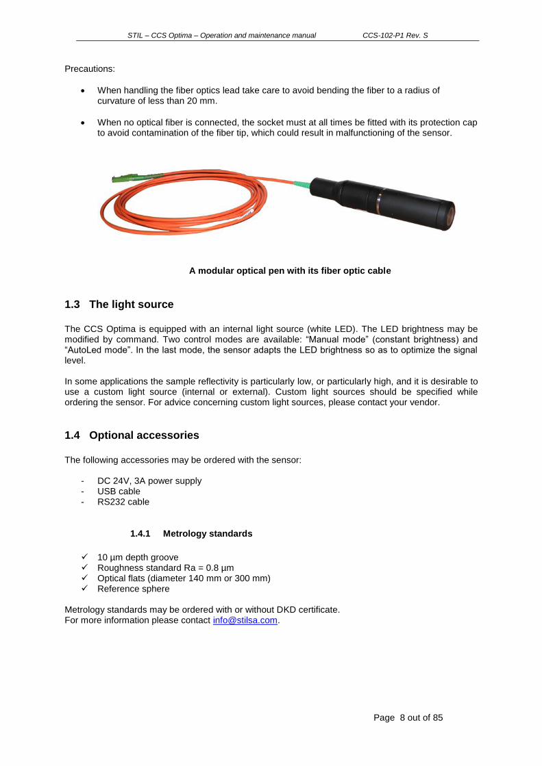
1.2 Optical pen and fiber optics
Optical pens are interchangeable: the same controller can store up to 20 different calibration tables corresponding to different optical pens. The optical pen is totally passive, since it incorporates no heat sources nor moving parts, thus avoiding any thermal expansion which could affect the accuracy of the sensor measuring process. The fiber optics cable which connects the optical pen to the controller may be ordered with a length up to 10 m. When handling the fiber optics lead take care to avoid bending the fiber to a radius of curvature of less than 20 mm.
STIL – CCS Optima – Operation and maintenance manual CCS-102-P1 Rev. S
Page 8 out of 85
Precautions:
When handling the fiber optics lead take care to avoid bending the fiber to a radius of curvature of less than 20 mm.
When no optical fiber is connected, the socket must at all times be fitted with its protection cap to avoid contamination of the fiber tip, which could result in malfunctioning of the sensor.
1.3 The light source
The CCS Optima is equipped with an internal light source (white LED). The LED brightness may be modified by command. Two control modes are available: “Manual mode” (constant brightness) and “AutoLed mode”. In the last mode, the sensor adapts the LED brightness so as to optimize the signal level. In some applications the sample reflectivity is particularly low, or particularly high, and it is desirable to use a custom light source (internal or external). Custom light sources should be specified while ordering the sensor. For advice concerning custom light sources, please contact your vendor.
1.4 Optional accessories
The following accessories may be ordered with the sensor:
- DC 24V, 3A power supply - USB cable - RS232 cable
1.4.1 Metrology standards
10 µm depth groove Roughness standard Ra = 0.8 µm Optical flats (diameter 140 mm or 300 mm) Reference sphere
Metrology standards may be ordered with or without DKD certificate. For more information please contact [email protected].
A modular optical pen with its fiber optic cable

STIL – CCS Optima – Operation and maintenance manual CCS-102-P1 Rev. S
Page 9 out of 85
2 Safety
The CCS Optima is an optoelectronic instrument. It is safe in normal operating conditions.
2.1 Electrical hazards
The CCS Optima controller box should be opened by qualified technicians only. Electrical hazards might exist, especially during an inappropriate intervention on the instrument. Unplug the instrument from the power outlet before changing accessories, maintenance, cleaning, or changing the lamp.
2.2 Optical hazards
The optical pen emits a beam of visible light with wavelengths ranging from 400 to 750 nm. The flux contained in this beam is smaller than the MPE (Maximum Permissible Exposure). However it is recommended to avoid looking directly into the optical pen.
2.3 General recommendations
Do not use the instrument if it has been dropped and shows signs of damage or functions improperly, or if the fan does not operate properly. In this case do not open the instrument and contact our helpline: [email protected] Repairs should only be carried out by qualified technicians using original replacement parts. In case of inappropriate use or failure to comply with the instructions, the manufacturer disclaims all liability and the guarantee will not apply.
2.4 Compliance with the EC regulation 89/336/EEC « Electromagnetic Compatibility »
The CCS Optima sensor complies with the generic or specific requirements of the following harmonized standards EN 50 081-1 Spurious emission EN 61000-6-2 Resistance to disturbance
2.5 Compliance with the RoHS Regulation
The CCS Optima is RoHS compliant.

STIL – CCS Optima – Operation and maintenance manual CCS-102-P1 Rev. S
Page 10 out of 85
3 Installation and startup
3.1 Electrical Connections
The following paragraphs explain how to:
Connect the sensor to a power supply
Connect the sensor to a host computer using either the RS232/RS422 port or the USB 2.0 port (the two ports may be connected simultaneously),
Connect the analog outputs,
Connect the synchronization signals,
Connect encoders for synchronous reading of position and sensor data
3.1.1 Power
Connect the power connector on the controller front panel to a to a DC 24V, 3A power supply. (Note: the black connector on the power socket may be screwed off the front panel and connected permanently to the power supply bare cables. Alternatively, a power supply may be ordered from the vendor).
3.1.2 RS232 – RS422 connector
The same connector is used for the RS232 link or RS422. The configuration is done through the interface connector, and more precisely with the last 2 pins (designated, respectively, “5V” and RS422). For RS232 interface these 2 pins should be left floating. For RS422 interface the 2 pins should be connected (RS422 pin connected to 5V pin). The RS232 RS422 connector is a RJ11 type connector. The pin out is described below: Front view:
RS232 pinout:
Pin Pin name Description for the CCS Optima
3 RX Receiver (Input)
4 Gnd
5 TX Transceiver (output)
RS422 pinout :
Pin Pin name Description for the CCS Optima
2 RX- Receiver - (Differential Input)
3 RX+ Receiver + (Differential Input)
4 Gnd
5 TX+ Transceiver + (Differential Output)
6 TX- Transceiver - (Differential Output)
STIL – CCS Optima – Operation and maintenance manual CCS-102-P1 Rev. S
Page 11 out of 85
3.1.3 USB connector
The USB 2.0 connector is a standard B-type connector. An USB 2.0 ( High-speed) compliant cable is required. (Note: A USB cable may be ordered from the vendor).
3.1.4 Analog outputs
The two 0V-10V Analog outputs are connected to pins 5 and 7 of the Interface connector, as indicated on the front panel. The “Set zero” button may be used to set the analog output zero level.
3.1.5 Synchronization signals
The Interface connector on the front panel of CCS Optima includes 3 pins dedicated to synchronization signals (TTL 0-5V): Pin n° 1: Sync in Pin n° 2: Ground Pin n° 3: Sync out
3.1.6 Encoder connector
The Encoder connector is a 20 points MDR connector (Manufacturer: 3M ; Reference 10220-6212PL). Pin out : 1 : Gnd 2 : a+ (axis 1) 3 : b+ (axis 1) 4 : a+ (axis 2)
5 : b+ (axis 2) 6 : a+ (axis 3) 7 : b+ (axis 3) 20 : 5 Vdc
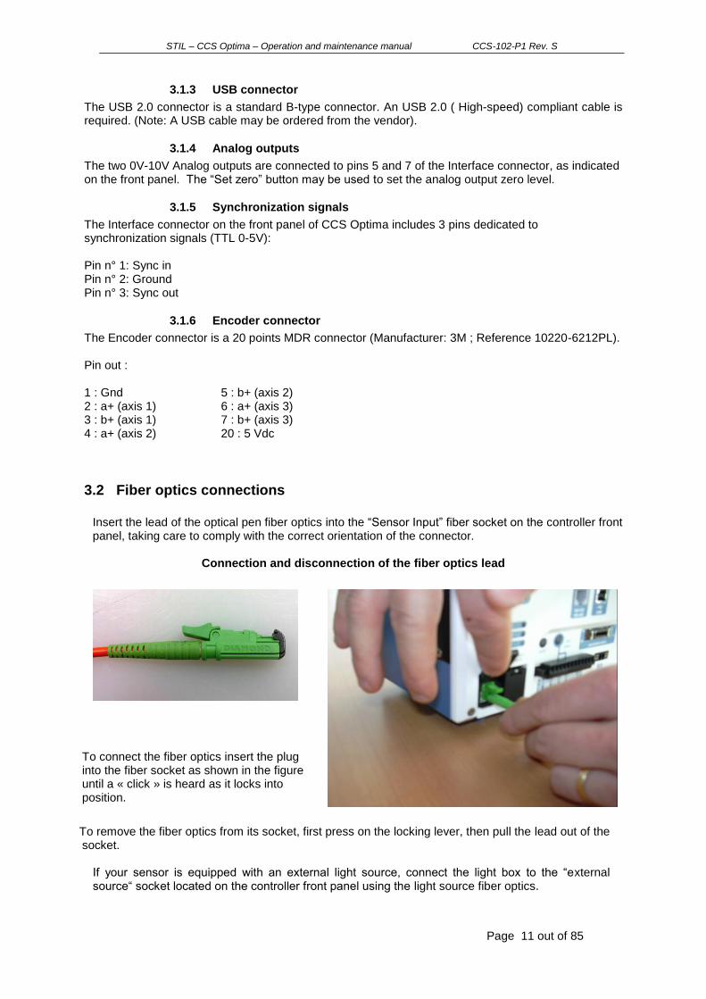
3.2 Fiber optics connections
Insert the lead of the optical pen fiber optics into the “Sensor Input” fiber socket on the controller front panel, taking care to comply with the correct orientation of the connector.
Connection and disconnection of the fiber optics lead
To connect the fiber optics insert the plug into the fiber socket as shown in the figure until a « click » is heard as it locks into position.
To remove the fiber optics from its socket, first press on the locking lever, then pull the lead out of the socket.
If your sensor is equipped with an external light source, connect the light box to the “external source“ socket located on the controller front panel using the light source fiber optics.

STIL – CCS Optima – Operation and maintenance manual CCS-102-P1 Rev. S
Page 12 out of 85
3.3 Installing the USB driver, the DLL and the “CCS Manager” software
3.3.1 Installing the USB driver:
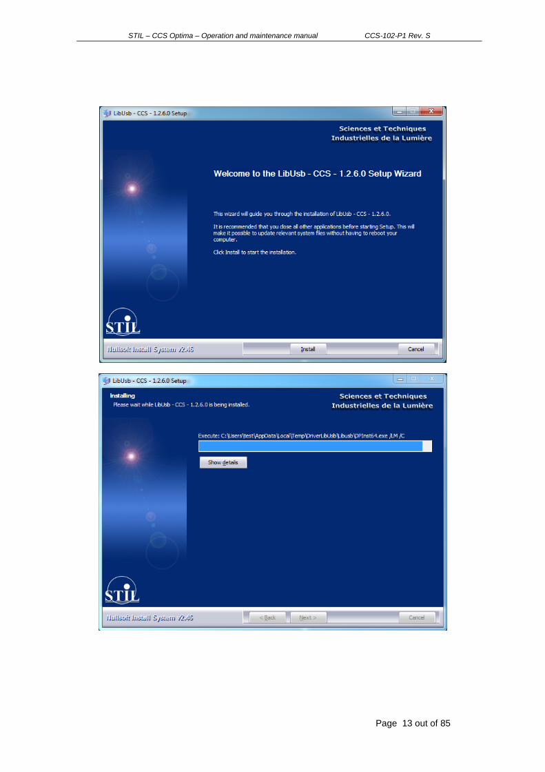
If you wish to communicate with the sensor using the USB port, you should install the dedicated USB driver on the host computer. The driver may be installed from the CD delivered with the sensor. Connect your sensor to the USB 2.0 port and switch it off. Insert the CD, and start the driver installation. Do not restart the sensor until prompted to do so by the installation program.
Use a host computer equipped with XP operating system with SP2, or Windows 7.
Insert the “CCS Manager” Utility CD into the CDROM drive. The Autorun screen appears:
Click on “USB drivers for CCS”
Select the language and continue as shown in the following screens:
STIL – CCS Optima – Operation and maintenance manual CCS-102-P1 Rev. S
Page 13 out of 85

STIL – CCS Optima – Operation and maintenance manual CCS-102-P1 Rev. S
Page 14 out of 85
After the driver‟s installation from the CD, the Windows “Add new Hardware wizard” starts. Select in the first window “Not this time” and in the following one “install automatically”. If the Windows wizard starts before or during STIL driver installation, leave it beside and come back to it when STIL driver installation is done.
3.3.2 Installing the software
From the Autorun screen, install the “CCS Manager” program. This program is used in the tutorial and the training sections.
If you intend to develop your own program for controlling the sensor, install the DLL SDK and/or the DOT NET Framework.
3.4 Sensor Startup
Startup procedure lasts about 10 seconds. The LED indicators on the sensor front panel go on and off, and the startup message indicating the firmware version is sent on the digital output channels, e.g.:
High Speed VART – COM Initiate< CCS V 1.2.56 CCS © 2006 FPGA : 010175 Booting sequence
At the end of the startup, the sensor starts measuring.

STIL – CCS Optima – Operation and maintenance manual CCS-102-P1 Rev. S
Page 15 out of 85
4 Basic Characteristics
The CCS OPTIMA is a high-resolution distance point-sensor. It is based on Chromatic Confocal Imaging (CSI). This chapter gives some basic notions concerning the technology, the applications and the measuring modes of the sensor.
4.1 Chromatic Confocal Imaging (CCI)
Chromatic Confocal Imaging is based on 2 principles:
Confocal imaging
Chromatic coding of the optical axis. The Confocal setup is an optical setup in which an optical system generates the image S‟ of a point source S on the surface of the object. The backscattered light is collected by the same optical system, which images the light spot on a pinhole S”. The pinhole is placed in front of a photodetector It filters the light rays that can reach the photodetector and for this reason it is also called “spatial filter”. Confocal setups are characterized by an exceptional Signal-to-Noise ratio. In the case of CCI the optical system is the chromatic optical pen and the photodetector is a spectrometer. Chromatic coding of the optical axis means that the optical system has axial chromatism: each wavelength is focalized at a different point along this axis. Suppose now that a sample is present
inside the chromatically-coded range so that the wavelength 0 is focalized on its surface. When the reflected (or backscattered) beam reaches the plane of the pinhole, the rays at wavelength are focalized on the pinhole so they can pass through the pinhole and reach the sensitive area of the spectrometer. Other wavelengths are imaged as large spots so they are blocked by the pinhole. The
spectrometer “decodes” the sample position by identifying the wavelength 0.
The spectrometer signal corresponds to the spectral repartition of the collected light. It presents a spectral peak. When the object moves inside the measuring range, the spectral peak on the spectrometer shifts.

STIL – CCS Optima – Operation and maintenance manual CCS-102-P1 Rev. S
Page 16 out of 85
4.2 Applications
Chromatic confocal sensors are used both in industrial environments for in-line inspection during production process, and in laboratory environments as high precision instruments. Their principal applications are:
Microtopography (measuring the shape of the sample),
Dimensional control (testing whether the size of certain features of manufactured products complies with specifications),
Quality control: (identification and characterization of defects on manufactured products),
Roughness measurement (measuring the statistical characteristics of the sample surface)
Tribology (characterization of mechanical or chemical erosion)
Thickness measurement. Chromatic confocal sensors are fully compatible with the ISO 25178 standard concerning the measurement and analysis of 3D a real surface texture. Moreover, Part 601 of this standard, dedicated to non-contact surface measurement, cites CCI as the first reference technology. Chromatic confocal sensors can measure samples made of practically any type of material (glass, ceramic, plastic, semiconductor, metal, fabric, paper, leather…). They can measure polished surfaces (mirrors, lenses, wafers) as well as rough ones.
The optical characteristics of the optical pen, and in particular the spot size, the axial resolution and the maximal slope angle, should be suited to the size and slope of the features present on the sample to be measured.
Metallic objects should be measured with the CL1 or the CL2 optical pens, in particular when measuring roughness or in applications requiring high resolution. When measuring metallic objects with optical pens whose spot size is larger, performances may fall short of specifications. The amount of degradation depends on microstructure of the metallic surface.
4.3 Measuring modes
Chromatic confocal sensors have two measuring modes : “Distance” and “Thickness”.
The principal measuring mode of the CCS OPTIMA is the “Distance” mode. The sensor is calibrated and tested in this mode. A calibration certificate attesting test results is delivered with the sensor.
The relation between the position of the spectral peak (“barycenter” in pixels) and the axial position of the object (“distance” in µm) is called “calibration lookup table” (LUT). The calibration LUT, characterizing a specific spectrometer and a specific optical pen, is measured by the fabricant and loaded into the controller
STIL – CCS Optima – Operation and maintenance manual CCS-102-P1 Rev. S
Page 17 out of 85
4.3.1 “Distance” measuring mode
In this mode the sensor measures the shape of a surface. This surface may be the outer surface of the sample or an inner interface. When measuring altitude profiles on an opaque sample (metal, paper, ceramics…), the use of the “Distance mode” is straightforward. When measuring thin transparent samples or coated samples it may happen that the sensor “sees” two signals at the same time: the coating surface reflects one signal and the substrate reflects a second one. By default the sensor selects the strongest signal and ignores all other detected signals, regardless of the relative positions of the spectral peaks. In some applications this behavior is not optimal: in the above example, the substrate reflectivity is often stronger than that of the coating, while one may wish to measure the coating surface. The “First peak” mode, described in the “Advanced Topics” chapter, gives a solution to such applications. (cf. §13.3 ) Like all photodetectors, the spectrometer signal comprises a certain amount of noise. In order to prevent false detections, peaks that are too week are filtered out using the “detection threshold” setting. The detection threshold is the minimal peak height, bellow which spectral peaks are considered as noise (cf. §13.1 )
4.3.2 “Thickness” measuring mode
The “Thickness” mode is an additional measuring mode dedicated to measuring the thickness of transparent samples. In this mode the sensor measures simultaneously the positions of the two faces of the transparent sample, and computes the thickness as the difference between these two positions. Measuring thickness is more difficult than measuring distance and is less precise. It is also subject to some limitations. In order to obtain metrological performances in this mode, a special procedure called “thickness calibration” should be carried out. Thickness calibration is performed by the user. This process requires a thickness standard. The “Thickness” measuring mode is described in §7.4
4.4 Measured data
At each point of the sample the sensor measures simultaneously several data. In the “Distance“ measuring mode the measured data are: the distance of the measured sample point the intensity of the retro-diffused light beam. In the thickness measuring mode the measured data are: the distance and intensity of the first sample face, the distance an intensity of he second sample face, the thickness. In addition to measured data the sensor may deliver some additional data (counter, state…). The sensor may be configured to transmit some or all of these data. (cf. §13.7)
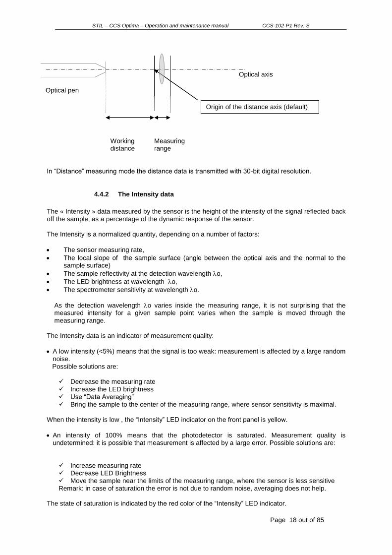
4.4.1 The distance data
The distance is null outside the measuring range. There is no way to tell if the sample is “too close” or “too far”: in both cases the measured distance is null. By default, the origin of the Distance axis is at the end of the Working Distance. Thus, the measured distance is larger for a sample point located on a “valley” than for a sample point located on a “hill”. The sense of the distance axis may be reversed using the RVS command, in which case the measured distance is larger for the “hill” and smaller for the “valley” (cf. §13.4). According to the distance sense, the distance data is referred to as “depth” or “altitude”.
STIL – CCS Optima – Operation and maintenance manual CCS-102-P1 Rev. S
Page 18 out of 85
In “Distance” measuring mode the distance data is transmitted with 30-bit digital resolution.
4.4.2 The Intensity data
The « Intensity » data measured by the sensor is the height of the intensity of the signal reflected back off the sample, as a percentage of the dynamic response of the sensor. The Intensity is a normalized quantity, depending on a number of factors:
The sensor measuring rate,
The local slope of the sample surface (angle between the optical axis and the normal to the sample surface)
The sample reflectivity at the detection wavelength o,
The LED brightness at wavelength o,
The spectrometer sensitivity at wavelength o.
As the detection wavelength o varies inside the measuring range, it is not surprising that the measured intensity for a given sample point varies when the sample is moved through the measuring range.
The Intensity data is an indicator of measurement quality:
A low intensity (<5%) means that the signal is too weak: measurement is affected by a large random noise.
Possible solutions are:
Decrease the measuring rate Increase the LED brightness Use “Data Averaging” Bring the sample to the center of the measuring range, where sensor sensitivity is maximal.
When the intensity is low , the “Intensity” LED indicator on the front panel is yellow.
An intensity of 100% means that the photodetector is saturated. Measurement quality is undetermined: it is possible that measurement is affected by a large error. Possible solutions are:
Increase measuring rate Decrease LED Brightness Move the sample near the limits of the measuring range, where the sensor is less sensitive Remark: in case of saturation the error is not due to random noise, averaging does not help.
The state of saturation is indicated by the red color of the “Intensity” LED indicator.
Optical axis
Optical pen
Working distance
Measuring range
Origin of the distance axis (default)

STIL – CCS Optima – Operation and maintenance manual CCS-102-P1 Rev. S
Page 19 out of 85
An intensity higher than 5% and lower than 100% indicates that measurement quality is correct. By adjusting the rate and the LED brightness as described in the tutorial it is possible to optimize the signal-to-noise ratio (SNR): so long as no saturation occurs, the SNR is roughly proportional to the square of the Intensity. A particular situation is the value of 99.0%. It indicates that the preprocessed signal is very high while the photodetector is not saturated. This situation corresponds to excellent measuring conditions.
When the intensity is correct, the “Intensity” LED indicator on the front panel is green.
4.4.3 Altitude images and Intensity images
In many applications it is desirable to obtain, in addition to the 3D measurement, a 2D image of the sample which resembles a microscope image. This can be done by scanning the sample and displaying the Intensity data. In fact the Intensity data gives exactly the same information as one pixel of a camera; by scanning one reconstructs the entire “image”. “Distance” images and “Intensity” images provide complementary information on the sample: the “Distance” image gives information on the altitude of each sample point, while the “Intensity” image gives information on the reflectivity of each sample point. “Distance” images are often displayed in false color or as 3D images, while “Intensity” images are usually displayed in grey-level or as “rendred” images simulating shadow effects. As an example, consider the following pairs of “Distance” and “Intensity” images.
“Distance” image (false color) and “Intensity” image (rendered image) of a microlens All measured data are available simultaneously, so the “distance” and “intensity” images may be obtained in a single scan.
4.5 External scanning
An important characteristics of the CCS OPTIMA sensor, is the fact that it is a “point” sensor; in other words, at any given instant the sensor measures a single point located on its optical axis. In order to obtain a profile or measure an entire surface, it is necessary to scan the sample along one or two axes with the aid of some external scanning device. Generally the scanning device is motorized; in some cases it comprises an encoder for determining the precise position of the sample at any given instant.

STIL – CCS Optima – Operation and maintenance manual CCS-102-P1 Rev. S
Page 20 out of 85
For some applications the synchronization between the sensor and the external scanning device is an important issue. The CCS OPTIMA may be synchronized both as a “slave” and as a “master”. This issue is described in chapter 12.
STIL – CCS Optima – Operation and maintenance manual CCS-102-P1 Rev. S
Page 21 out of 85
5 Communication with the CCS Optima
There are 3 options for communicating with the CCS Optima sensor:
“CCS Manager”
a) The “CCS Manager” software may be used to configure the sensor very easily and to view, save and print the measured data. It features a “Command Terminal” for sending commands to the sensor, and allows uploading new firmware versions. The application comprises special procedures for in-situ calibration and for generating refractive index files. In case you have a problem with the sensor, this software can generate with a single mouse click a diagnostics data file with all sensor parameters. Please join the diagnostics file to any technical question addressed to your vendor.
DLLs The « CHR DLL» may be used to interface the sensor with a general-purpose user program. The DLL is intended for user programs in C or C++ language. Its operating manual includes a large number of code samples. The “STIL Sensor DLL” is intended for all .NET compatible languages (Labview, VB, C# C++/CLI, etc.).
Low-level communication using the digital I/O: The RS232/RS422 serial link and the USB link enable sensor configuration using a specific control language, and acquisition of the measured data. As an example, the Windows™ « Hyper Terminal »™ utility can be used for sending commands via the RS232 link and for receiving the measurements back from the sensor. The Command Terminal of the “CCS Manager” software can be used with either RS232 or USB.
The serial link allows baud rates up to 460800. For this link there exist some limitations on the amount of data transmissible simultaneously (cf. §9.2). USB allows unlimited data transmission at all rates.
Recommendation: All software applications use the same COM port or USB port to communicate with the sensor. Remember to always free the port by quitting one application before attempting to connect it to another application.
Important: For communication using the USB port, a dedicated USB driver should be installed on the host device (cf. §3.3)
The “CCS Manager” software and the DLL SDK are free software packages supplied with the sensor. They are common to all STIL point sensors (CCS Optima, STIL Initial, STIL-DUO…). They may be installed from the CD delivered with the sensor. Requirements: Windows XP SP3 or Windows Seven, 32 bits or 64 bits.

STIL – CCS Optima – Operation and maintenance manual CCS-102-P1 Rev. S
Page 22 out of 85
6 Getting started (Tutorial 1)
This chapter is a tutorial intended for new users to familiarize themselves with the main characteristics of the CCS Optima sensor. For simplification purposes, this tutorial only introduces one measuring mode (« Distance » mode) and one communication option (the «CCS Manager» software and the USB digital output). We recommend that new users follow this tutorial even if they wish subsequently to use a different measuring mode or another communication option.
6.1 Connecting to the CCS Optima
Connect the sensor to a power supply as described in §3.1.1. Connect it to a free USB 2.0 port of your computer as described in §3.1.3. Make sure the dedicated USB driver and the CCS Manager software have been previously installed on the computer (cf. §3.3)
Switch the sensor on and start the “CCS Manager” program. This program has 4 access levels.
The “Operator” level requires no password. This levels allows configuring the sensor, launching a measurement, viewing and saving the data as time-profiles.
The “User” level requires a password – please contact your vendor to receive it. The “User” level allows, in addition to the above operations, viewing the photodetector signal. The 2 other levels are reserved. For this tutorial you can enter either in the “Operator” level or in the “User” level.
The “Connection wizard” window opens.
The program will scan all available USB ports on the host computer until it finds the sensor and will start the connection process, including download of the entire sensor configuration. Note: If you wish to connect to the serial link, click on “Parameters” and check the “Serial link” option, and then click on “Connect”. The program saves the last connection parameters.

STIL – CCS Optima – Operation and maintenance manual CCS-102-P1 Rev. S
Page 23 out of 85
The “CCS Manager” Main Window appears: It comprises a menu and 2 data frames on the top, a status bar at the bottom, page-selection buttons and a “Dark” button on the left, a central zone for displaying the current page, and two data bar graphs.
Note: the “Signal” page-selection button does not appear in the “Operator” level.
6.2 Configuring the sensor
Click on the « Configuration » button on the left side of the Main Window to develop the arborescence of configuration pages (1 “Basic” page, 5 “Advanced” pages and 1 “Expert” page)
Select the “Basic” configuration page.
Page- selection Buttons
Menu
Data 1 Frame Data 2 Frame
Data 2 Bar-graph
Data 1 Bargraph
Data 1 Selection
Data 2 Selection
Current Page (here « Measurement » Page)
Dark Button
Status Bar
STIL – CCS Optima – Operation and maintenance manual CCS-102-P1 Rev. S
Page 24 out of 85
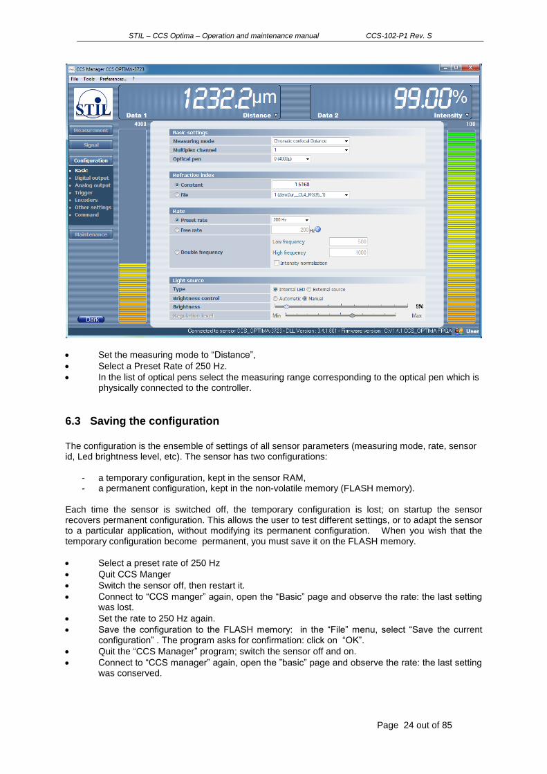
Set the measuring mode to “Distance”,
Select a Preset Rate of 250 Hz.
In the list of optical pens select the measuring range corresponding to the optical pen which is physically connected to the controller.
6.3 Saving the configuration
The configuration is the ensemble of settings of all sensor parameters (measuring mode, rate, sensor id, Led brightness level, etc). The sensor has two configurations:
- a temporary configuration, kept in the sensor RAM, - a permanent configuration, kept in the non-volatile memory (FLASH memory).
Each time the sensor is switched off, the temporary configuration is lost; on startup the sensor recovers permanent configuration. This allows the user to test different settings, or to adapt the sensor to a particular application, without modifying its permanent configuration. When you wish that the temporary configuration become permanent, you must save it on the FLASH memory.
Select a preset rate of 250 Hz
Quit CCS Manger
Switch the sensor off, then restart it.
Connect to “CCS manger” again, open the “Basic” page and observe the rate: the last setting was lost.
Set the rate to 250 Hz again.
Save the configuration to the FLASH memory: in the “File” menu, select “Save the current configuration” . The program asks for confirmation: click on “OK”.
Quit the “CCS Manager” program; switch the sensor off and on.
Connect to “CCS manager” again, open the ”basic” page and observe the rate: the last setting was conserved.

STIL – CCS Optima – Operation and maintenance manual CCS-102-P1 Rev. S
Page 25 out of 85
6.4 Selecting the output data
The CCS transmits several data items for each measured point. Before launching a measurement, you should check that the data item/s you wish to measure are directed to the right output port (the USB port or the Serial port), and that the other data items are not transmitted. On the left side of the Main Window, select the “Digital Output” page.
First, observe the list of available data items in the “Distance” measuring mode. In this mode you can measure the Distance and the Intensity of the reflected signal. The other data items in the list will be described later so for the moment we shall content ourselves with a brief presentation:
The “Distance LSB” data comprises additional 15-bit resolution to the “Distance” data. This topic is described in §9.1.2. For the moment, each time you select the “Distance” data, select this data as well.
The “Barycenter” data is the position (pixel number) of the spectral peak on the photodetector.
The “Counter” data is a 15-bit cyclic counter incremented at each measured point: this data is supplied as a tool for software developers. This data is particularly useful in the case of “trigger modes”.
The “Adaptive mode” data and the “State” data are described in the “Advanced Topics” chapter. Next, set the measuring mode to “Thickness”. In this mode you measure the two faces of a transparent sample, so you have 2 Distances, 2 Intensities and 2 Barycenters
Recommendation: When you find the optimal settings which suit your application, save the configuration on the sensor FLASH Memory so that the sensor always starts with this “nominal” configuration.

STIL – CCS Optima – Operation and maintenance manual CCS-102-P1 Rev. S
Page 26 out of 85
In the screen copy above, The thickness and the intensities are directed to the RS232, while the 2 distances are directed to USB. In this way one can connect the sensor to 2 applications simultaneously (e.g. HyperTerminal on the serial port and CCS manager on the USB port). Note: Encoder data may be transmitted simultaneously with other data regardless of measuring mode. Transmission is enables and disabled from the “Encoder” page. To finish, return to the “Distance” measuring mode which is the principal measuring mode of the sensor. Set the “Distance”, “Intensity” and “Counter” data to “USB”, and the other data to “Not Transmitted”. On the left side of the Main Window, select the “Measurement” page.
6.5 Viewing and saving the measured data
Each “Data frame” allows choosing one data among the data transmitted to the connected port. If you have selected “Distance”, “Intensity” and “Counter” data, you may display one of these data as Data1, and another one as Data2. To do so, click on the small farrow on the right-bottom corner of the Data frame (just below the unit) to see the list of available data, and select the desired data. If you do not see the desired data in the list return to the “Digital output” page and direct it to the connected port. Select data1 as “Distance” ; In the “Data 2” frame Select “Intensity”. Note that each of data1 and data2 is displayed in 3 ways:
- Digitally, in the “Data frame” - As a bar-graph (to the left and to the right of the graphic window, respectively)
Graphically, in the graphic window of the Measurement page. The buttons at the top of the “Measurement” give access to the following functions:
- Start and stop the measurement - Print, Save and Clear the graphics window - Find the curve at high zoom values - See the statistics of the last measurement - Modify the number of displayed points

STIL – CCS Optima – Operation and maintenance manual CCS-102-P1 Rev. S
Page 27 out of 85
Data 1 scale
Time (horizontal axis) slide
Data 1 slide
Data 1 zoom
Data 2 slide
Data 2 scale
Data 2 curve
Time (horizontal axis) zoom Data 1 display toggle
Number of displayed points (horiz. Axis)
Data 2 zoom
« Clear graphics » button
« Recenter graphics » button
« Start/Stop » button
« Print graph» button
« Save graph » button

STIL – CCS Optima – Operation and maintenance manual CCS-102-P1 Rev. S
Page 28 out of 85
To save the measured data, use the “save graph” icon. Data may be saved either as a screen-copy (bitmap) or as digital data (text file).
6.6 Acquiring the Dark signal
The dark signal of the sensor is generated by undesirable back-reflections on the optical surfaces inside the sensor. This signal must be measured and saved to the non-volatile memory so that it can be subtracted from the measured signal. The level of the Dark signal depends on the sampling rate and on the LED brightness. A dark signal acquisition is performed during adjustment by the manufacturer, but must be repeated at regular intervals.
Recommendation: The dark signal acquisition procedure should preferably be performed at least a quarter of an hour after switching on the sensor, in order to ensure that sensor has reached thermal equilibrium.
Dark signal measurement may be launched either by pressing the “Dark” button on the sensor front panel, or by clicking on the “Dark” button on the “CCS Manager” software, or, more generally, by sending the “$DRK” command to the sensor. This operation may take a few dozens of seconds, as the sensor measures and saves the “Dark” signal at all pre-set frequencies successively. In order to perform a dark signal acquisition, it is essential to have no object within the measurement field, or even better, to blank off the light beam by applying a piece of paper over the tip of the optical pen. Press the “Dark” button on the front panel of the sensor. The “Intensity” and “Measure” Led indicators on the front panel blink on and off in green alternatively, to indicate that the operation is in progress. Keep the optical pen tip blanked off. When measurement is done, the 3 LED indicators blink on and off simultaneously, and their color indicates the result of the operation:
Green if the level of the acquired dark signal is satisfactory at all rates Orange if the dark signal level is too high at low rates, but it is still possible to measure at
higher rates Red if the dark signal level is too high at all rates.
The piece of paper can now be removed and the sensor can be used in the normal way.
6.6.1 Related topics
“Fast” Dark cf § 8.2
Note that each data has its own scale, zoom factor and slide. To access the zoom, click on the point at the upper end of the scale. You may also zoom with the mouse button.

STIL – CCS Optima – Operation and maintenance manual CCS-102-P1 Rev. S
Page 29 out of 85
High Dark signal If on completion of the dark acquisition sequence the color of the blinking LED Indicators is orange or red, this means that the acquired dark signal is too high. In this case it is not possible to configure the sensor to the lowest measuring rate (or rates). If the problem persists, see instructions in the “Maintenance” chapter (cf. §16.2).
6.7 Adjusting the LED brightness
Internal LEDS brightness may be controlled by command. There are two modes for doing this: “Manual” and “Automatic”. This section describes the Manual mode. The “Automatic” LED mode is described in the “Advanced Topics” chapter. The LED emission is modulated at a high rate (100 kHz). The effective brightness is determined by the cycle ratio (percentage of the exposure time for which the LED is on).
Set the level control to “Manual” and move the Brightness slide to the right until the brightness level is 100%.
Place a piece of white paper in front of the optical pen and observe the spot of light emitted by the sensor. Move the paper forward and backward to find the focus plane where the spot brightness is maximal.
Move the brightness slide to the left to get a brightness level of 0%. The light spot disappears.
Try intermediate values
To finish, set the LED to maximal brightness again.
6.7.1 Minimal brightness level
For each frequency there exists a minimal brightness level below which the LED cannot go:
Measuring Rate Minimal brightness level
Maximal brightness level
Up to 2000 Hz 10% 100%
2000 Hz – 10000 Hz 20% 100%
The operator sets the LED to level X The sensor behavior:
X = 0% The LED goes off
X ≤ Minimal level The LED is practically set to the minimal level
X > Minimal level The LED is set to level X
6.8 Placing the sample within the measurement range of the optical pen
Mount the optical pen on a suitable support (for example, a « V » shape block). Position the sample to be measured in front of the pen, and move it forward or backward until the optical pen working distance is reached. For pens with a millimetric measurement range, the positioning of the sample within the measurement range of the optical pen is easy to achieve, simply observe on the sample surface or on a piece of white paper the luminous spot emitted by the optical pen: as the measuring range is approached, the spot becomes smaller and smaller and its intensity increases.
STIL – CCS Optima – Operation and maintenance manual CCS-102-P1 Rev. S
Page 30 out of 85
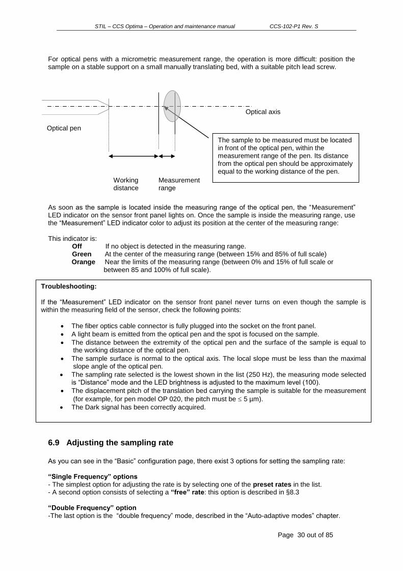
For optical pens with a micrometric measurement range, the operation is more difficult: position the sample on a stable support on a small manually translating bed, with a suitable pitch lead screw. As soon as the sample is located inside the measuring range of the optical pen, the “Measurement” LED indicator on the sensor front panel lights on. Once the sample is inside the measuring range, use the “Measurement” LED indicator color to adjust its position at the center of the measuring range: This indicator is: Off If no object is detected in the measuring range.
Green At the center of the measuring range (between 15% and 85% of full scale) Orange Near the limits of the measuring range (between 0% and 15% of full scale or between 85 and 100% of full scale).
6.9 Adjusting the sampling rate
As you can see in the “Basic” configuration page, there exist 3 options for setting the sampling rate: “Single Frequency” options - The simplest option for adjusting the rate is by selecting one of the preset rates in the list. - A second option consists of selecting a “free” rate: this option is described in §8.3 “Double Frequency” option -The last option is the “double frequency” mode, described in the “Auto-adaptive modes” chapter.
The sample to be measured must be located in front of the optical pen, within the measurement range of the pen. Its distance from the optical pen should be approximately equal to the working distance of the pen.
Optical axis
Optical pen
Working distance
Measurement range
Troubleshooting: If the “Measurement” LED indicator on the sensor front panel never turns on even though the sample is within the measuring field of the sensor, check the following points:
The fiber optics cable connector is fully plugged into the socket on the front panel.
A light beam is emitted from the optical pen and the spot is focused on the sample.
The distance between the extremity of the optical pen and the surface of the sample is equal to the working distance of the optical pen.
The sample surface is normal to the optical axis. The local slope must be less than the maximal slope angle of the optical pen.
The sampling rate selected is the lowest shown in the list (250 Hz), the measuring mode selected is “Distance” mode and the LED brightness is adjusted to the maximum level (100).
The displacement pitch of the translation bed carrying the sample is suitable for the measurement
(for example, for pen model OP 020, the pitch must be 5 µm).
The Dark signal has been correctly acquired.
STIL – CCS Optima – Operation and maintenance manual CCS-102-P1 Rev. S
Page 31 out of 85
In this tutorial we shall use preset rates only. When the sample is within the central part of measurement range of the optical pen, select the optimal preset rate in the list: the signal should be strong but not saturated. You can know if the signal is too strong or too weak by watching the “Intensity” LED indicator. This indicator is:
Off if no signal is detected Red in case of signal saturation Green if signal intensity is comfortable (> 5% of the maximum level), Orange if signal intensity is low (< 5% of the maximum level)
If the indicator is red, you should increase the sampling rate or decrease the LED brightness; if it is orange you should lower the sampling rate or increase the LED brightness. The first Tutorial is over. We recommend the user to get some practice with the features dealt with in this tutorial before starting the second tutorial.
Recommendation: Always set the Rate and the LED Brightness so that the “Intensity” LED Indicator is green. When the signal is low (yellow “Intensity” LED Indicator) or saturated (red “Intensity” LED Indicator) the sensor still measures, but measurement quality may be deteriorated.
STIL – CCS Optima – Operation and maintenance manual CCS-102-P1 Rev. S
Page 32 out of 85
7 Going further (Tutorial 2)
This chapter is a tutorial intended for users having acquired some initial experience with the CCS Optima sensor in the « Distance » measuring mode and using the « CCS Manager » application. This tutorial covers the following topics:
Synchronizing the sensor with external devices: - Synchronizing the sensor with digital encoders - Synchronization signals and « Trigger » modes
More about the “CCS Manger” program - Help Utility - Communication with the sensor via the “CCS Manager” Command Terminal - The “Tools” menu
Communication with the sensor via RS232 serial link using the Windows « Hyper Terminal »™ utility.
The “Thickness” measuring mode
7.1 Synchronizing the sensor with other devices
It is often necessary to synchronize the sensor with an external device, such as an encoder, a motion controller or a photocell indicating the approach of an object traveling on a conveyor belt.
When the external device to be synchronized with the sensor is a digital encoder, this task is particularly easy, as it is performed automatically by the CCS Optima (cf. §12)
For other types of devices (analog encoders, motion controllers) synchronization may be achieved using synchronization signals and Trigger modes. The CCS Optima may be synchronized with an external device as “master” (using the “Sync out” TTL signals), as a “slave” (using the “Sync in” TTL signals), or in a mixed mode (using both types of signals). “Trigger modes” specify the way the sensor should respond to rising or falling edges of the “Sync in” signals. The common feature to all trigger modes is that the sensor stops measuring and stands by for an “active” edge on “Sync in” connector. Trigger modes may be enabled and disabled from the “Trigger” page of the “CCS manager” program, by the DLL or by low-level commands. By default, all trigger modes are disabled, and the sensor transmits data without interruption immediately after startup. When no trigger mode is enabled, rising and falling edges of the “Sync in” signal are simply ignored.
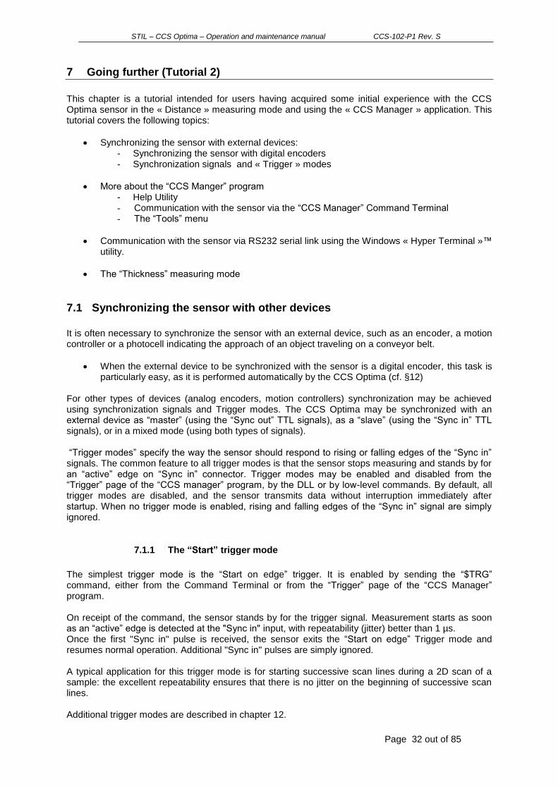
7.1.1 The “Start” trigger mode
The simplest trigger mode is the “Start on edge” trigger. It is enabled by sending the “$TRG” command, either from the Command Terminal or from the “Trigger” page of the “CCS Manager” program. On receipt of the command, the sensor stands by for the trigger signal. Measurement starts as soon as an “active” edge is detected at the "Sync in" input, with repeatability (jitter) better than 1 µs. Once the first "Sync in" pulse is received, the sensor exits the “Start on edge” Trigger mode and resumes normal operation. Additional "Sync in" pulses are simply ignored. A typical application for this trigger mode is for starting successive scan lines during a 2D scan of a sample: the excellent repeatability ensures that there is no jitter on the beginning of successive scan lines. Additional trigger modes are described in chapter 12.

STIL – CCS Optima – Operation and maintenance manual CCS-102-P1 Rev. S
Page 33 out of 85
7.1.2 Training
Connect an optical pen to the sensor; configure the sensor to the right optical pen and to « Distance» measuring mode as described in the first tutorial. Launch a « Dark » signal measurement.
Place a sample in the measurement range of the pen and adjust the sampling rate and/or the LED intensity.
Connect the « Sync in » pins on the Interface connector to an adjustable external signal (for example, a TTL 0-5V pulse generator) as described in §3.1. Check that the signal is on 0V.
Select the “Trigger” page of the “CCS Manager” software. Select the “Start” trigger type and rising edge as the “active” edge. Click on the “Enable the selected mode” button to enable the mode.
Select the “Measurement” page. Set Data 1 to “Distance” and the number of points to 100, and click several times on the “Start” button.. If previous steps have been carried out correctly, nothing happens: no data is displayed in the Graphic window as the sensor is in standby for a “Sync in” signal.
Send a TTL pulse to the “Sync In” input in order to trigger the measurement: data transmission starts immediately.
Check that the measurement is not stopped: the “Start/stop” button should look as following:

STIL – CCS Optima – Operation and maintenance manual CCS-102-P1 Rev. S
Page 34 out of 85
7.2 Learning more about the “CCS Manager” software
7.2.1 Help utility
To learn more about “CCS Manager” features, click on the “?” icon in the Menu, and open the “Help” utility. In particular, we recommend reading the sections concerning the ““Maintenance”, the Configuration “Other Settings” page and the “Analog Data” page, which are not described in this tutorial.
7.2.2 Command Terminal
Open the “Expert” Configuration page.
Type $AVR25 (6 characters:$ sign, 3 upper case letters, and 2 digits) in the “Command” line, and click on the “Send” button. This command sets the temporal averaging to 25. As a result, for each 25 successive points the sensor sends a single value. As a result data transmission is 25 times slower and the signal to noise ratio is improved by a factor of 5 (5 = square root of 25).
Watch the sensor reply in the “Sensor response” line.
Type $MOD0 ($ sign, 3 upper case letters and 1 digit), and click on the “Send” button. This command selects the “Distance” measuring mode. Watch the sensor reply in the “Sensor response” line.
Type $BAU115200 , and click on the “Send” button. This command sets the baud rate to 115200. Watch the sensor reply in the “Sensor response” line.
Type $ASC, and click on the “Send” button. This command configures the sensor in « ASCII » mode.
STIL – CCS Optima – Operation and maintenance manual CCS-102-P1 Rev. S
Page 35 out of 85
The Terminal allows communicating with the sensor using the specific CCS command language. Commands are described in detail later on in this manual. For the moment, note that commands begin by a $ sign, comprise 3 upper case letters, and end with the numerical value of the parameter. The sensor echoes the command and then sends “ready”. Note the button “Reload sensor parameters” bellow the command terminal. This button uploads the configuration again, so that the “CCS Manager” program will refresh its parameter list in order to take the modifications following the commands into account. This button has no effect on the sensor, it effects only the “CCS Manger” user interface.
7.2.3 Tools Menu
7.2.4 Preferences Menu
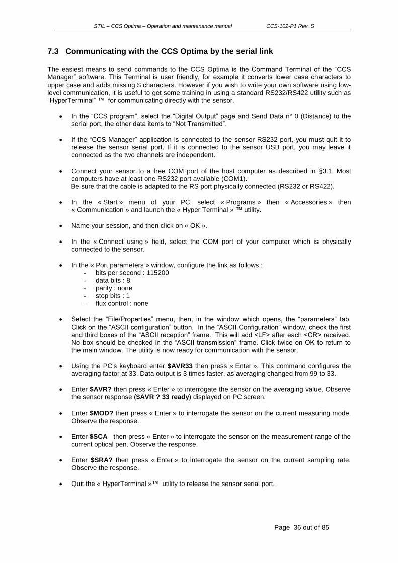
The “Preferences” menu gives access to the following parameters: - Language - Auto connect on startup - Invert distance - Convert to inches - Choose a Zero - Add an Offset - Check for update
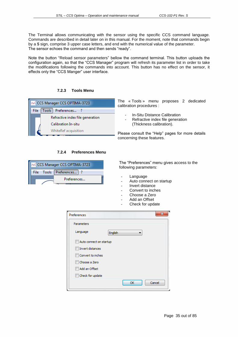
The « Tools » menu proposes 2 dedicated calibration procedures :
- In-Situ Distance Calibration - Refractive index file generation
(Thickness calibration). Please consult the “Help” pages for more details concerning these features.
STIL – CCS Optima – Operation and maintenance manual CCS-102-P1 Rev. S
Page 36 out of 85
7.3 Communicating with the CCS Optima by the serial link
The easiest means to send commands to the CCS Optima is the Command Terminal of the “CCS Manager” software. This Terminal is user friendly, for example it converts lower case characters to upper case and adds missing $ characters. However if you wish to write your own software using low-level communication, it is useful to get some training in using a standard RS232/RS422 utility such as “HyperTerminal” ™ for communicating directly with the sensor.
In the “CCS program”, select the “Digital Output” page and Send Data n° 0 (Distance) to the serial port, the other data items to “Not Transmitted”.
If the “CCS Manager” application is connected to the sensor RS232 port, you must quit it to release the sensor serial port. If it is connected to the sensor USB port, you may leave it connected as the two channels are independent.
Connect your sensor to a free COM port of the host computer as described in §3.1. Most computers have at least one RS232 port available (COM1). Be sure that the cable is adapted to the RS port physically connected (RS232 or RS422).
In the « Start » menu of your PC, select « Programs » then « Accessories » then « Communication » and launch the « Hyper Terminal » ™ utility.
Name your session, and then click on « OK ».
In the « Connect using » field, select the COM port of your computer which is physically connected to the sensor.
In the « Port parameters » window, configure the link as follows : - bits per second : 115200 - data bits : 8 - parity : none - stop bits : 1 - flux control : none
Select the “File/Properties” menu, then, in the window which opens, the “parameters” tab. Click on the “ASCII configuration” button. In the “ASCII Configuration” window, check the first and third boxes of the “ASCII reception” frame. This will add <LF> after each <CR> received. No box should be checked in the “ASCII transmission” frame. Click twice on OK to return to the main window. The utility is now ready for communication with the sensor.
Using the PC's keyboard enter $AVR33 then press « Enter ». This command configures the averaging factor at 33. Data output is 3 times faster, as averaging changed from 99 to 33.
Enter $AVR? then press « Enter » to interrogate the sensor on the averaging value. Observe the sensor response ($AVR ? 33 ready) displayed on PC screen.
Enter $MOD? then press « Enter » to interrogate the sensor on the current measuring mode. Observe the response.
Enter $SCA then press « Enter » to interrogate the sensor on the measurement range of the current optical pen. Observe the response.
Enter $SRA? then press « Enter » to interrogate the sensor on the current sampling rate. Observe the response.
Quit the « HyperTerminal »™ utility to release the sensor serial port.

STIL – CCS Optima – Operation and maintenance manual CCS-102-P1 Rev. S
Page 37 out of 85
7.4 Measuring thickness
This mode is useful for measuring the thickness of singal-layer transparent samples. The sensor searches for two spectral peaks, generated, respectively, by light reflections (or backscattering) on the two faces of the transparent sample. If two peaks are detected as expected, the sensor calculates the distance and the intensity of face 1 (front face, i.e. the nearest face), the distance and intensity of face 2 (rear face), and the thickness. All these data are available simultaneously. The signification of the distance data and the intensity data is the same as in CCI/Distance mode. The data “Distance2” and “Thickness” depend on the “refractive index” parameter. For these data to true, the sensor should be configured to the correct refractive index. In particular, in CCI mode, the measured thickness is proportional to the “refractive index” parameter. Remark: due to the refractive index, the measured Thickness and Distance 2 may be larger than the measuring range.
7.4.1 Thickness calibration (refractive index file generation)
In order to get metrological accuracy in CCI/Thickness mode, it is necessary to carry out a procedure called “thickness calibration” using a standard (artifact) with a known thickness. The procedure consists of moving the sample throughout the measuring range and computing a correction coefficient at each position. This procedure generates a “refractive index” file which specifies an effective refractive index value for each position in the measuring range. The file is specific to a given sample type (e.g. a 3 mm BK7 glass) and a given sensor. The “CCS manager” software comprises a utility for generating refractive index files (accessible from the “Tools” menu). Please refer to the “Help” utility of this software for a detailed description of this procedure. The sensor can hold up to 8 refractive index files in its non-volatile memory. Existing files may be selected in the “Basic” configuration file of “CCS manager” or by command. For applications which do not require metrological accuracy, thickness may be measured with no calibration, by specifying an average refractive index for the visual band. The accuracy obtained without calibration is of the order or 1%- 2%.
7.4.2 Minimum measurable thickness
The thickness of the sample to be measured must be greater than or equal to the “Min Measureable Thickness” of the optical pen. The « Min Measurable Thickness » limit is specified in the in the e-catalog that you may find in our website www.stilsa.com. If the sample thickness is smaller than this limit, the two spectral peaks are so close that the sensor is unable to resolve them, so it considers them as a single peak. The min measurable thickness is proportional to the refractive index of the measured material. The values in the e-catalog are for samples with a refractive index of 1.5. When measuring the thickness of an air-gap (refractive index=1.0) the specified value should be divided by 1.5.
7.4.3 Maximal measurable thickness
Important: To obtain a valid measurement in « Thickness » mode, the sensor should be configured to the correct refractive index.
=
LCD DISPLAY
+
KEYPAD
wn.

STIL – CCS Optima – Operation and maintenance manual CCS-102-P1 Rev. S
Page 38 out of 85
The thickness of the sample to be measured must be smaller than or equal to the “Max Measureable Thickness” of the optical pen. The « Max Measurable Thickness » limit is specified in the in the e-catalog that you may find in our website www.stilsa.com. If the sample thickness is larger than this limit, the two spectral peaks are so far that at least one of them is outside the measuring range of the optical pen. The max measurable thickness is proportional to the refractive index of the measured material. The values in the e-catalog are for samples with a refractive index of 1.5. When measuring the thickness of an air-gap (refractive index=1.0) the specified value should be divided by 1.5.
7.4.4 Smoothing
In most situations the measurement signal to noise ratio (SNR) is improved by applying a smoothing filter on the measured spectrum. However, for measuring a sample whose thickness is close to the min measurable thickness, better results are obtained by de-activating the default smoothing. (cf. §13.2)
7.4.5 Single surface in “Thickness” mode
It may happen that a single surface is detected while the sensor is configured to “Thickness” mode. This may occur if one or the other of the sample faces is outside the measuring range, if one of the signals is too weak, or if the thickness is smaller than the “Minimal measurable thickness” of the optical pen. In the latter case the sensor fails to resolve the two surfaces and considers them as a single one. The “Unmeasured peak handling” (cf. $12.5) command determines the behavior of the sensor in such a case. The default behavior is: the data relative to face 2 is set equal to the data of face 1, and the thickness is set to zero.
7.4.6 Measuring the Thickness of opaque samples
The “Thickness” mode can only be used for transparent thickness whose thickness is compatible with the min and max measurable thickness of the optical pen. For measuring the thickness of opaque samples, the most frequently used method consists of using two sensors looking at each other and located on both sides of the sample with collinear optical axes. Both sensors are configured to “Distance” mode. The Thickness of the sample is given by: Thickness = K – (D1 + D2) Where D1 and D2 are the distances measured by the two sensors and the constant K is determined using a standard with known thickness.
7.4.7 Training
In the “Basic” page, set the measuring mode to Thickness. Set the “refractive index” parameter value to the average refractive index of the sample in the visible range. (If you do not know the precise value, leave it at its default value). In the “Digital output” page, select Data n° 0 (Thickness). Set the other data to “Not Transmitted”
Recommendation: In « Thickness » mode, place the sample in the center of the measuring range to avoid having either one of the faces close to the limits of the range.

STIL – CCS Optima – Operation and maintenance manual CCS-102-P1 Rev. S
Page 39 out of 85
Place a thickness sample in the measurement range of the optical pen, such as a glass slide, a piece of cellophane, a transparent plastic film or any other flat transparent sample. If it is a sheet or a film, ensure it is pulled tight. Also check that the axis of the optical pen is normal to the surface of the sample. The sample thickness must be compatible with the thickness measuring range of the optical pen.
In the “Measurement” page set the number of points to 3000, and click on “Start”.
Move the optical pen slowly backward and forward to bring the two faces of the sample inside the measuring range. As soon as the sample is inside the measuring range, non-zero thickness values appear in the Graphic window.
Note that of the “Measure” LED-indicator depends only on the presence and position of the first peak, it does not tell if a second peak has been detected.
Note that the displayed thickness values are proportional to the refractive index value.
The second Tutorial is over, you are ready now to start your own application.
Troubleshooting: If you succeed to obtain a measurement in “Distance” measuring mode, but in “Thickness” measuring mode the measured thickness is zero, check the following points:
The thickness of the sample must be compatible with the measurement range limits
The sample must be sufficiently transparent.
The sample must be pulled tight.
The optical axis must be normal to the surface of the sample.
The sampling rate selected must be the lowest in the list
The two faces of the sample must be inside the measuring range

STIL – CCS Optima – Operation and maintenance manual CCS-102-P1 Rev. S
Page 40 out of 85
PART II: BASIC FEATURES
8 Main functions of the CCS Optima
8.1 Optical pen selection
The CCS Optima sensor may accept up to 20 calibration tables corresponding to 20 different optical pens. The optical pen can be selected in the “Basic” configuration page of CCS Manager, or by sending the „Select confocal sensor‟ command.
8.1.1 Optical pen selection The „Select confocal sensor‟ command is used to specify or to request the index of the calibration table corresponding to optical pen connected to the CCS.
Select confocal sensor
Function Set/request the index of the calibration table
Command $SENn or $SEN ?
Parameter/Value returned n = index of the table (2 digit integer between 0 and 19)
Example $SEN04
8.1.2 Full scale value of the optical pen currently selected This command is used to get the measurement range of the currently selected optical pen.
Scale
Function Request the measurement range of the current optical pen
Command $SCA
Value returned measurement range in microns
8.1.3 List of optical pens This command is used to get the list of calibration tables and the measuring ranges of the corresponding optical pens.
List
Function Request the list of measuring ranges of the 20 calibration ranges
Command $LUL
Value returned List of 20 measuring ranges, in microns
8.2 Dark signal
The Function of the « Dark » signal is explained in the « Getting started » chapter. Dark acquisition may be launched using the “Dark” button on the sensor front panel, from the “CCS Manger” Main Window, or by sending a „Dark‟ command.
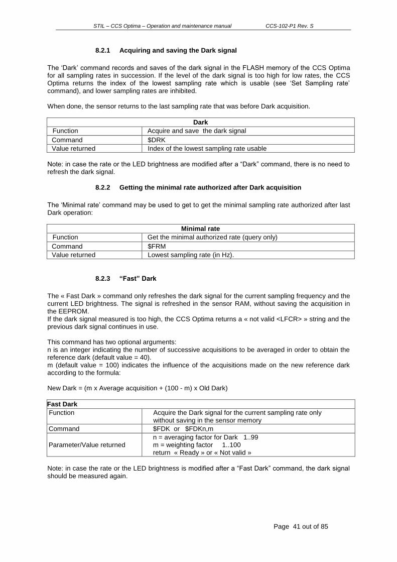
STIL – CCS Optima – Operation and maintenance manual CCS-102-P1 Rev. S
Page 41 out of 85
8.2.1 Acquiring and saving the Dark signal
The „Dark‟ command records and saves of the dark signal in the FLASH memory of the CCS Optima for all sampling rates in succession. If the level of the dark signal is too high for low rates, the CCS Optima returns the index of the lowest sampling rate which is usable (see „Set Sampling rate‟ command), and lower sampling rates are inhibited. When done, the sensor returns to the last sampling rate that was before Dark acquisition.
Dark
Function Acquire and save the dark signal
Command $DRK
Value returned Index of the lowest sampling rate usable
Note: in case the rate or the LED brightness are modified after a “Dark” command, there is no need to refresh the dark signal.
8.2.2 Getting the minimal rate authorized after Dark acquisition
The „Minimal rate‟ command may be used to get to get the minimal sampling rate authorized after last Dark operation:
Minimal rate
Function Get the minimal authorized rate (query only)
Command $FRM
Value returned Lowest sampling rate (in Hz).
8.2.3 “Fast” Dark
The « Fast Dark » command only refreshes the dark signal for the current sampling frequency and the current LED brightness. The signal is refreshed in the sensor RAM, without saving the acquisition in the EEPROM. If the dark signal measured is too high, the CCS Optima returns a « not valid <LFCR> » string and the previous dark signal continues in use. This command has two optional arguments: n is an integer indicating the number of successive acquisitions to be averaged in order to obtain the reference dark (default value = 40). m (default value = 100) indicates the influence of the acquisitions made on the new reference dark according to the formula: New Dark = (m x Average acquisition + (100 - m) x Old Dark)
Fast Dark
Function Acquire the Dark signal for the current sampling rate only without saving in the sensor memory
Command $FDK or $FDKn,m
Parameter/Value returned n = averaging factor for Dark 1..99 m = weighting factor 1..100 return « Ready » or « Not valid »
Note: in case the rate or the LED brightness is modified after a “Fast Dark” command, the dark signal should be measured again.

STIL – CCS Optima – Operation and maintenance manual CCS-102-P1 Rev. S
Page 42 out of 85
8.3 Sampling rate
In the “Single Frequency” mode the sampling rate of the sensor may be managed by 2 methods:
Selection of a preset sampling rate from a list (“Preset Rate”)
Definition of a specific sampling rate (“Free rate” or “Exposure Time”)
The first method, which is simple and easy to use, is recommended for most applications. In this method, the sampling rate is defined by its index. The second method provides greater flexibility in the choice of sampling rate: The “free” sampling rate can be specified in Hz, or the exposure time (inverse of the free rate) can be specified in µs. This paragraph describes the different methods, followed by some examples. The “Double Frequency” mode is described in the “Auto-adaptive Modes” chapter.
8.3.1 Selecting a preset sampling rate
The CCS Optima provides the following preset sampling rates
Index Sampling rate (HZ) Exposure time (µs)
00 free rate Free exposure time
01 250 4000
02 500 2000
03 1000 1000
04 2000 500
05 5000 200
06 10000 10
A preset rate may be selected from the “Basic” configuration page of “CCS Manager”, or by sending the „Preset Rate‟ command.
Preset Rate
Function Set/request the index of a preset sampling rate
Command $SRAn or $SRA?
Parameter/Value returned n = sampling rate index (2 digit integer 0 - 5) Note: limited by the min authorized rate
Note: the command $SRA0 selects the free rate. The value attributed to the free rate may be set by the “Free rate” command or by the “Exposure time“ command described below.
8.3.2 “Free” sampling rate
A free rate may be selected from the “Basic” configuration page of “CCS Manager”, or by sending the „Free Rate‟ command. The „Free Rate‟ command is used to set the sensor sampling rate to a free value between 250 Hz and 10000 Hz, or to request the value of the free rate. The index of the free rate in the list of preset rates is 0 (see table above). The last value set to the free rate either by the “Free Rate” command or by the “Exposure time” command may be later activated by sending “$SRA0”.
Note: The Processor may modify slightly the specified value of free rate in order to comply with its internal constraints (the exposure time in µs should be integer), and returns the real value immediately after the echo (see example bellow).

STIL – CCS Optima – Operation and maintenance manual CCS-102-P1 Rev. S
Page 43 out of 85
Free rate
Function Set/request the value in Hz of the free rate.
Command $FRQn or $FRQ?
Parameter n = value of the free sampling rate, in Hz, limited by the min authorized rate
Value returned 5 digit integer between 250 and 10000
Example Command: $FRQ1995 Response: $FRQ1995 1996 Note: 1996 Hz corresponds to an integer exposure time (501 µs).
8.3.3 Exposure time
The „Exposure time‟ command is used to set/request the free exposure time in µs. The free sampling rate is set to 1 000 000/exposure time.
Exposure time
Function Set/request the exposure time
Command $TEXn or $TEX?
Parameter n = value of the free exposure time, in µs (5 digit integer between 00010 and 04000), limited by the min authorized rate.
Examples In the following dialog the operator alternates “Preset rate”, “Free Rate” and “Exposure Time” commands, and interrogates the sensor to view the results of each command. Read this dialog carefully and make sure you understand the response of the sensor in each case.
Command Comment Response from the sensor
$SRA03 Sets the preset sampling rate index to 3 (1000 Hz)
$SRA 03<CR> ready
$SRA? Interrogates the sensor for the index of the current preset sampling rate
$SRA?03 ready
$FRQ? Interrogates the sensor for the rate in Hz $FRQ?01000 ready
$TEX? Interrogates the sensor for the exposure time in µs 1000 = 1 000 000/ 1000
$TEX?01000 ready
$TEX00530 Sets exposure time to 530 µs (and sets the sampling rate index to 0)
$TEX00530<CR>00530 ready
$FRQ? Interrogates the sensor for the rate in Hz 1886 = 1 000 000/ 530
$FRQ? 1886
$SRA? Interrogates the sensor for the index of the current preset sampling rate
SRA? 00 ready
$FRQ1995 Sets the free rate to 1995 Hz The sensor selects a close value (1996)
$FRQ1995 <CR> 1996
$TEX? Interrogates the sensor for the exposure time in µs 501 = 1 000 000/ 1996
$TEX?00501
$TEX00120 Attempts to set exposure time to a non-authorized value
$TEX120 not valid ready
$ SRA01 Sets the preset sampling rate index to 1 (250 Hz) This ends the “free rate” mode
$SRA01 <CR> ready
$FRQ? Interrogates the sensor for the rate in Hz
FRQ?00250 ready
$SRA00 Sets the preset sampling rate index to 0 (“free rate”)
$SRA00 <CR> ready
$FRQ? Interrogates the sensor for the rate in Hz 1996 is the last value attributed to the free rate
$FRQ? 1996

STIL – CCS Optima – Operation and maintenance manual CCS-102-P1 Rev. S
Page 44 out of 85
8.4 Measuring modes
The different measuring modes are described in the „Going further „chapter.
Index 0 1
Measuring mode Distance Thickness
The measuring mode can be selected from the “Basic” configuration page of “CCS manger” or by sending the „Mode‟ command.
Measuring Mode
Function Set/request the current measuring mode
Command $MODn or $MOD?
Value returned n = Id of the measuring mode (0-1)
8.5 Refractive index
The sample refractive index is necessary in the “Thickness” measuring mode. Refractive index can be set from the “Basic” configuration page of “CCS manger” or by sending the „Refractive Index‟ command.
8.5.1 Setting a constant refractive index
8.5.2 Selecting a Refractive index file
Refractive index file are used to describe the variation of refractive index within the measuring range (cf. “Advanced Topics”). The “Refractive index file” command is used to load a previously saved refractive index file.
Note the material name “CONSTIND” attributed in case the file id is 0.
Refractive Index
Function Set/request the sample refractive index
Command $SRIx or $SRI?
Value returned x = sample refractive index (up to 5 decimal digits) 1.0 <= x < 10.0
Example $SRI1.512, $SRI1.6478
Refractive index file
Function Set/request the sample refractive index
Command $INFn
Parameter n = 0 : constant refractive index (determined by last SRI command) n=1..8 : id of an existing refractive index file
Values returned s: file name x1,x2,x3: the minimal, the maximal and the average refractive index values in the file
Example
Command: $INF3 or $INF? Response: $INF3,”BK7”, 1.50900, 1.52531, 1.51330 -------------------------------------------------------------------------------------- Command: $INF0 Response: $INF0,”CONSTIND”,1.5200,1.5200,1.5200
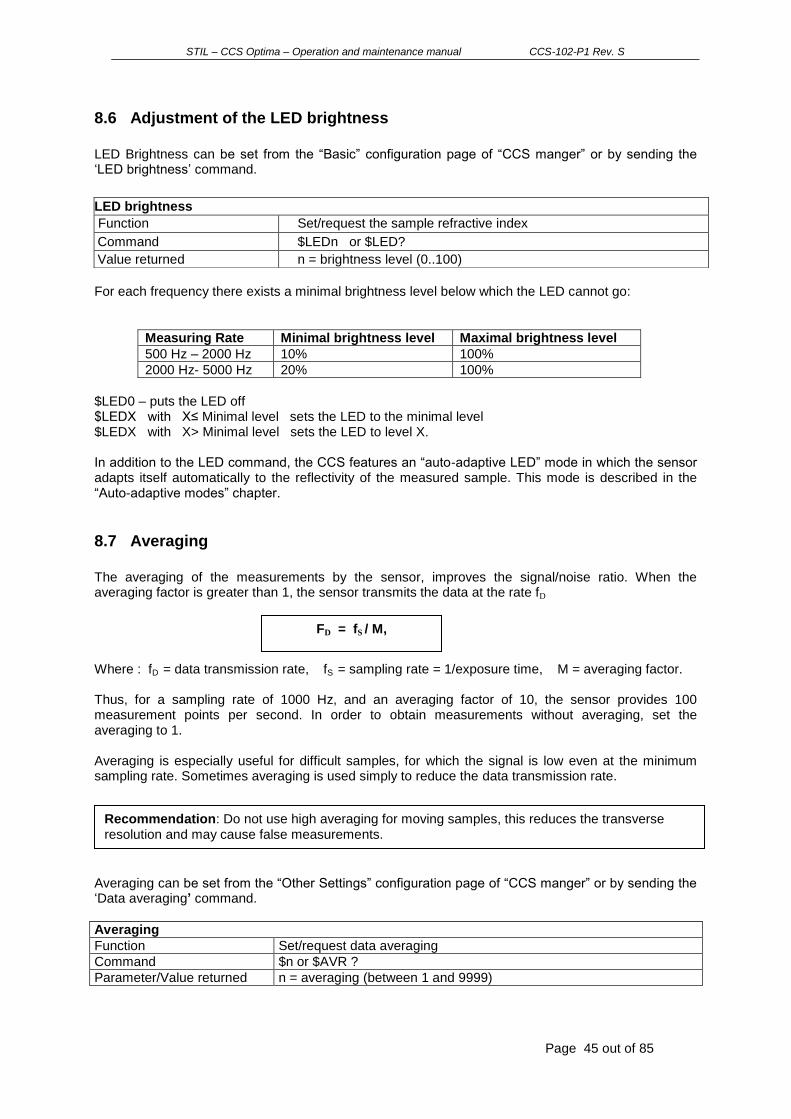
STIL – CCS Optima – Operation and maintenance manual CCS-102-P1 Rev. S
Page 45 out of 85
8.6 Adjustment of the LED brightness
LED Brightness can be set from the “Basic” configuration page of “CCS manger” or by sending the „LED brightness‟ command.
For each frequency there exists a minimal brightness level below which the LED cannot go:
Measuring Rate Minimal brightness level Maximal brightness level
500 Hz – 2000 Hz 10% 100%
2000 Hz- 5000 Hz 20% 100%
$LED0 – puts the LED off $LEDX with X≤ Minimal level sets the LED to the minimal level $LEDX with X> Minimal level sets the LED to level X. In addition to the LED command, the CCS features an “auto-adaptive LED” mode in which the sensor adapts itself automatically to the reflectivity of the measured sample. This mode is described in the “Auto-adaptive modes” chapter.
8.7 Averaging
The averaging of the measurements by the sensor, improves the signal/noise ratio. When the averaging factor is greater than 1, the sensor transmits the data at the rate fD Where : fD = data transmission rate, fS = sampling rate = 1/exposure time, M = averaging factor. Thus, for a sampling rate of 1000 Hz, and an averaging factor of 10, the sensor provides 100 measurement points per second. In order to obtain measurements without averaging, set the averaging to 1. Averaging is especially useful for difficult samples, for which the signal is low even at the minimum sampling rate. Sometimes averaging is used simply to reduce the data transmission rate.
Averaging can be set from the “Other Settings” configuration page of “CCS manger” or by sending the „Data averaging’ command.
Averaging
Function Set/request data averaging
Command $n or $AVR ?
Parameter/Value returned n = averaging (between 1 and 9999)
LED brightness
Function Set/request the sample refractive index
Command $LEDn or $LED?
Value returned n = brightness level (0..100)
FD = fS / M,
Recommendation: Do not use high averaging for moving samples, this reduces the transverse resolution and may cause false measurements.
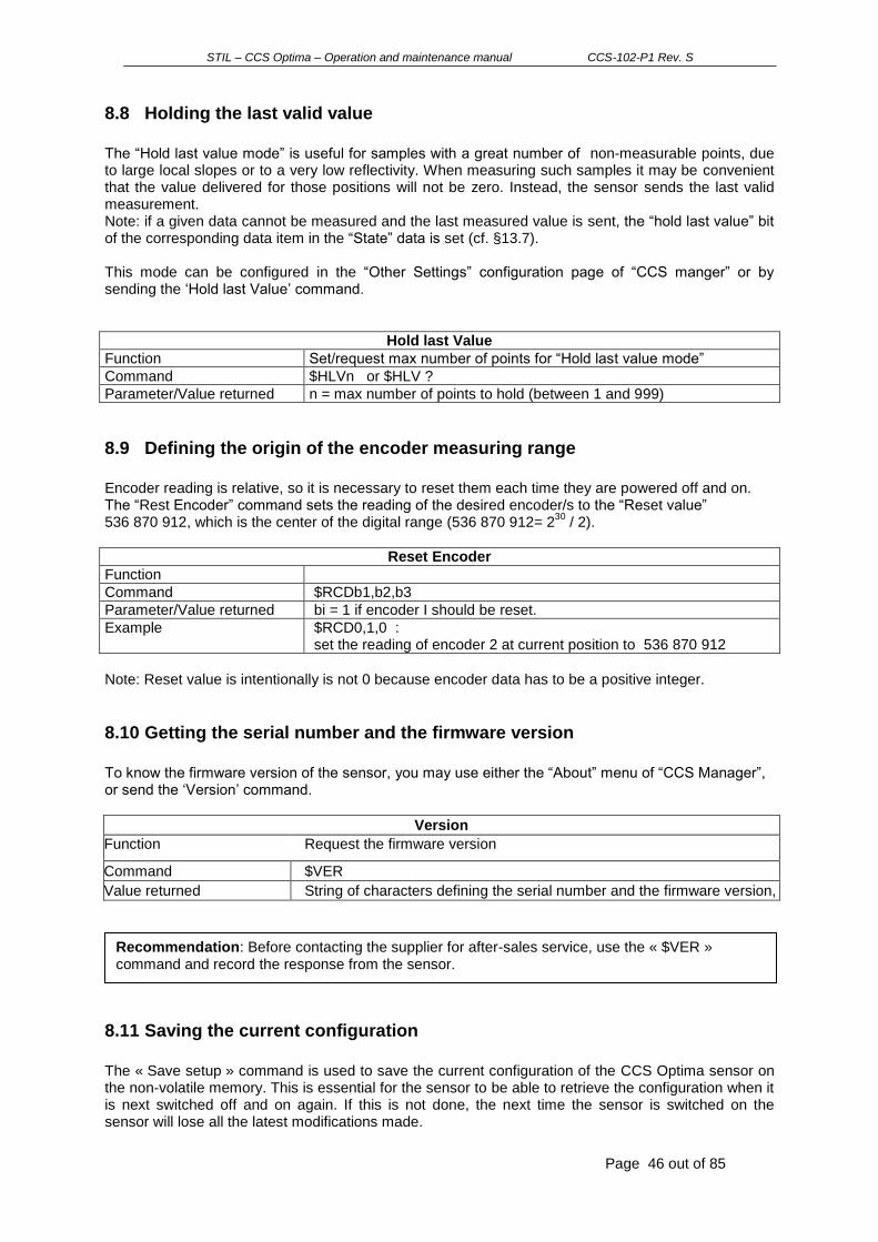
STIL – CCS Optima – Operation and maintenance manual CCS-102-P1 Rev. S
Page 46 out of 85
8.8 Holding the last valid value
The “Hold last value mode” is useful for samples with a great number of non-measurable points, due to large local slopes or to a very low reflectivity. When measuring such samples it may be convenient that the value delivered for those positions will not be zero. Instead, the sensor sends the last valid measurement. Note: if a given data cannot be measured and the last measured value is sent, the “hold last value” bit of the corresponding data item in the “State” data is set (cf. §13.7). This mode can be configured in the “Other Settings” configuration page of “CCS manger” or by sending the „Hold last Value‟ command.
Hold last Value
Function Set/request max number of points for “Hold last value mode”
Command $HLVn or $HLV ?
Parameter/Value returned n = max number of points to hold (between 1 and 999)
8.9 Defining the origin of the encoder measuring range
Encoder reading is relative, so it is necessary to reset them each time they are powered off and on. The “Rest Encoder” command sets the reading of the desired encoder/s to the “Reset value” 536 870 912, which is the center of the digital range (536 870 912= 2
30 / 2).
Reset Encoder
Function
Command $RCDb1,b2,b3
Parameter/Value returned bi = 1 if encoder I should be reset.
Example $RCD0,1,0 : set the reading of encoder 2 at current position to 536 870 912
Note: Reset value is intentionally is not 0 because encoder data has to be a positive integer.
8.10 Getting the serial number and the firmware version
To know the firmware version of the sensor, you may use either the “About” menu of “CCS Manager”, or send the „Version‟ command.
Version
Function Request the firmware version
Command $VER
Value returned String of characters defining the serial number and the firmware version,
8.11 Saving the current configuration
The « Save setup » command is used to save the current configuration of the CCS Optima sensor on the non-volatile memory. This is essential for the sensor to be able to retrieve the configuration when it is next switched off and on again. If this is not done, the next time the sensor is switched on the sensor will lose all the latest modifications made.
Recommendation: Before contacting the supplier for after-sales service, use the « $VER » command and record the response from the sensor.
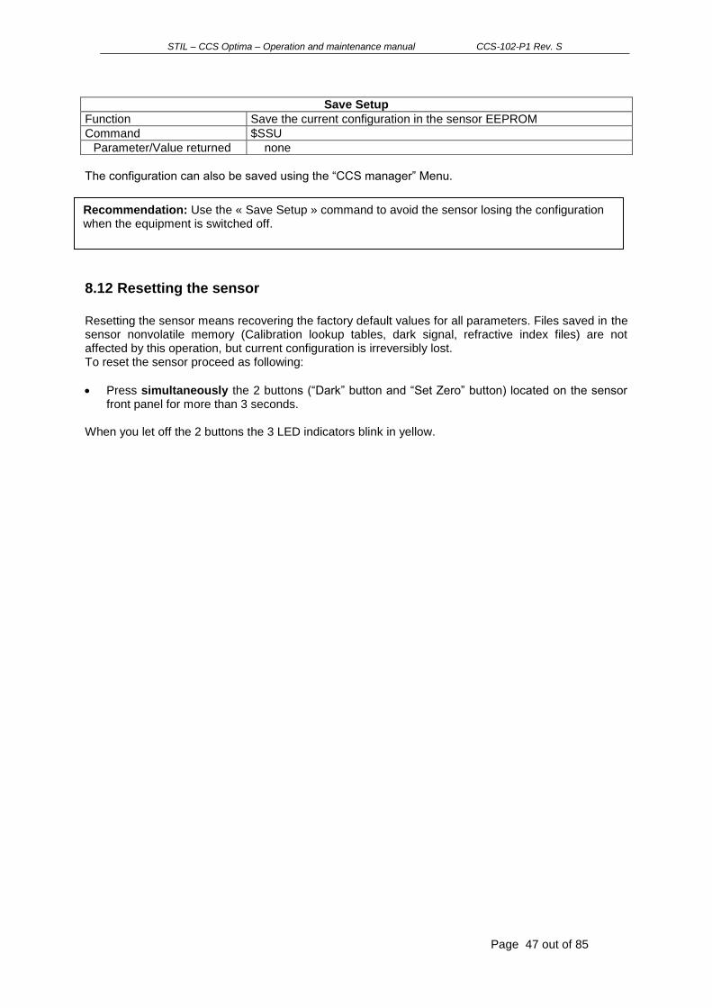
STIL – CCS Optima – Operation and maintenance manual CCS-102-P1 Rev. S
Page 47 out of 85
The configuration can also be saved using the “CCS manager” Menu.
8.12 Resetting the sensor
Resetting the sensor means recovering the factory default values for all parameters. Files saved in the sensor nonvolatile memory (Calibration lookup tables, dark signal, refractive index files) are not affected by this operation, but current configuration is irreversibly lost. To reset the sensor proceed as following:
Press simultaneously the 2 buttons (“Dark” button and “Set Zero” button) located on the sensor front panel for more than 3 seconds.
When you let off the 2 buttons the 3 LED indicators blink in yellow.
Save Setup
Function Save the current configuration in the sensor EEPROM
Command $SSU
Parameter/Value returned none
Recommendation: Use the « Save Setup » command to avoid the sensor losing the configuration when the equipment is switched off.
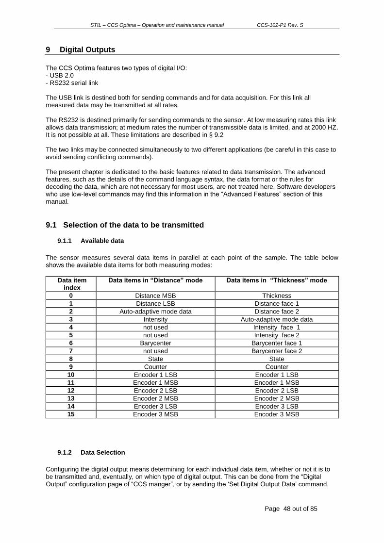
STIL – CCS Optima – Operation and maintenance manual CCS-102-P1 Rev. S
Page 48 out of 85
9 Digital Outputs
The CCS Optima features two types of digital I/O: - USB 2.0 - RS232 serial link The USB link is destined both for sending commands and for data acquisition. For this link all measured data may be transmitted at all rates. The RS232 is destined primarily for sending commands to the sensor. At low measuring rates this link allows data transmission; at medium rates the number of transmissible data is limited, and at 2000 HZ. It is not possible at all. These limitations are described in § 9.2 The two links may be connected simultaneously to two different applications (be careful in this case to avoid sending conflicting commands). The present chapter is dedicated to the basic features related to data transmission. The advanced features, such as the details of the command language syntax, the data format or the rules for decoding the data, which are not necessary for most users, are not treated here. Software developers who use low-level commands may find this information in the “Advanced Features” section of this manual.
9.1 Selection of the data to be transmitted
9.1.1 Available data
The sensor measures several data items in parallel at each point of the sample. The table below shows the available data items for both measuring modes:
Data item index
Data items in “Distance” mode Data items in “Thickness” mode
0 Distance MSB Thickness
1 Distance LSB Distance face 1
2 Auto-adaptive mode data Distance face 2
3 Intensity Auto-adaptive mode data
4 not used Intensity face 1
5 not used Intensity face 2
6 Barycenter Barycenter face 1
7 not used Barycenter face 2
8 State State
9 Counter Counter
10 Encoder 1 LSB Encoder 1 LSB
11 Encoder 1 MSB Encoder 1 MSB
12 Encoder 2 LSB Encoder 2 LSB
13 Encoder 2 MSB Encoder 2 MSB
14 Encoder 3 LSB Encoder 3 LSB
15 Encoder 3 MSB Encoder 3 MSB
9.1.2 Data Selection
Configuring the digital output means determining for each individual data item, whether or not it is to be transmitted and, eventually, on which type of digital output. This can be done from the “Digital Output” configuration page of “CCS manger”, or by sending the „Set Digital Output Data‟ command.

STIL – CCS Optima – Operation and maintenance manual CCS-102-P1 Rev. S
Page 49 out of 85
Set Digital Output Data
Function Set/request which data is to be transmitted via the serial link.
Command $SOD n0,n1,n2,n3,n4,n5,n6,n7,n8,n9,n10,n11,n12,n13,n14,n15 or $SOD ?
Parameter/Value returned
Ni = 0 (data not transmitted), or 1 (data transmitted on RS serial link), or 9 (data transmitted on USB) i = 0..15 (index of the data item)
It is possible to specify the ports of the first data only. In this case the last data remain unchanged e.g. “ $SOD9,0,0,9” specifies the digital ports of the first 4 data and leaves the others unchanged.
Trouble shooting:
$SOD1 is not equivalent to $SOD1,0,0,0,0,0,0,0,0,0,0,0,0,0,0,0 Example: If you send $SOD9,0,0,9 followed by $SOD1 and then send the query $SOD? The sensor responds $SOD1,0,0,9,0,0,0,0,0,0,0,0,0,0,0,0
Examples:
In « Distance» measuring mode, for the sensor to transmit the values of the Distance and Intensity at each measurement via the RS link, the following command must be sent : $SOD1,1,0,1
In « Distance» measuring mode, for the sensor to transmit the value of the Distance only via the USB link, the following command must be sent : $SOD 9,9
In “Thickness” measuring mode, for the sensor to transmit the Thickness on USB and the Counter on RS232, the following command must be sent : SOD9,0,0,0,0,0,0,0,0,1
9.2 Specific features of the RS232 / RS422 link
The RS232 /RS422 connector at the CCS Optima controller front panel should be connected to a free COM Port on the host computer or on the device used for communicating with the sensor, using a direct (non-crossed) serial link wire as described in §3.1. No specific driver is required. The baud rate of the sensor RS link should be matched to that of the host computer.
9.2.1 Configuring of the COM port of the host computer
The host computer COM port should be configured as follows:
Data bits : 8
Warning: For the RS link the transmission capacity depends on the sampling rate and the data format (see further in this chapter). Before sending the $SOD command, check that the number of data items selected is compatible with these parameters in order to avoid data overflow. There is no limitation on the number of transmitted data items for the USB link.
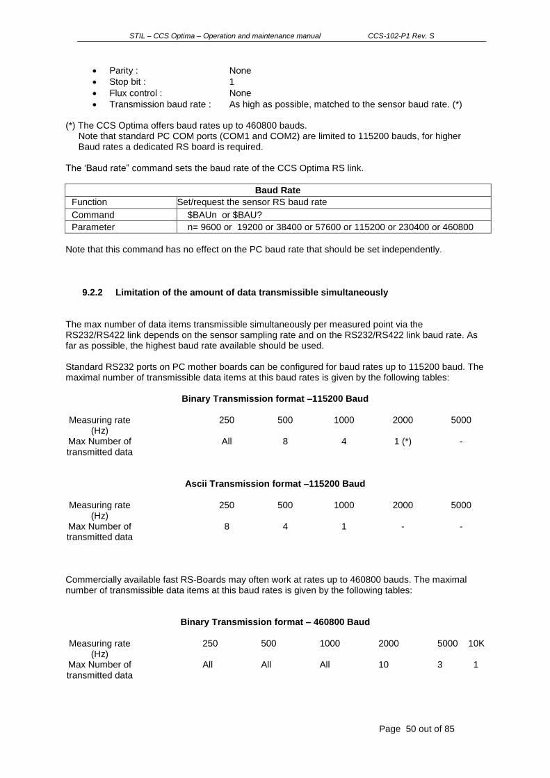
STIL – CCS Optima – Operation and maintenance manual CCS-102-P1 Rev. S
Page 50 out of 85
Parity : None
Stop bit : 1
Flux control : None
Transmission baud rate : As high as possible, matched to the sensor baud rate. (*) (*) The CCS Optima offers baud rates up to 460800 bauds. Note that standard PC COM ports (COM1 and COM2) are limited to 115200 bauds, for higher Baud rates a dedicated RS board is required. The „Baud rate” command sets the baud rate of the CCS Optima RS link.
Baud Rate
Function Set/request the sensor RS baud rate
Command $BAUn or $BAU?
Parameter n= 9600 or 19200 or 38400 or 57600 or 115200 or 230400 or 460800
Note that this command has no effect on the PC baud rate that should be set independently.
9.2.2 Limitation of the amount of data transmissible simultaneously
The max number of data items transmissible simultaneously per measured point via the RS232/RS422 link depends on the sensor sampling rate and on the RS232/RS422 link baud rate. As far as possible, the highest baud rate available should be used. Standard RS232 ports on PC mother boards can be configured for baud rates up to 115200 baud. The maximal number of transmissible data items at this baud rates is given by the following tables:
Binary Transmission format –115200 Baud Measuring rate
(Hz) 250 500 1000 2000 5000
Max Number of transmitted data
All 8 4 1 (*) -
Ascii Transmission format –115200 Baud Measuring rate
(Hz) 250 500 1000 2000 5000
Max Number of transmitted data
8 4 1 - -
Commercially available fast RS-Boards may often work at rates up to 460800 bauds. The maximal number of transmissible data items at this baud rates is given by the following tables:
Binary Transmission format – 460800 Baud Measuring rate
(Hz) 250 500 1000 2000 5000 10K
Max Number of transmitted data
All All All 10 3 1
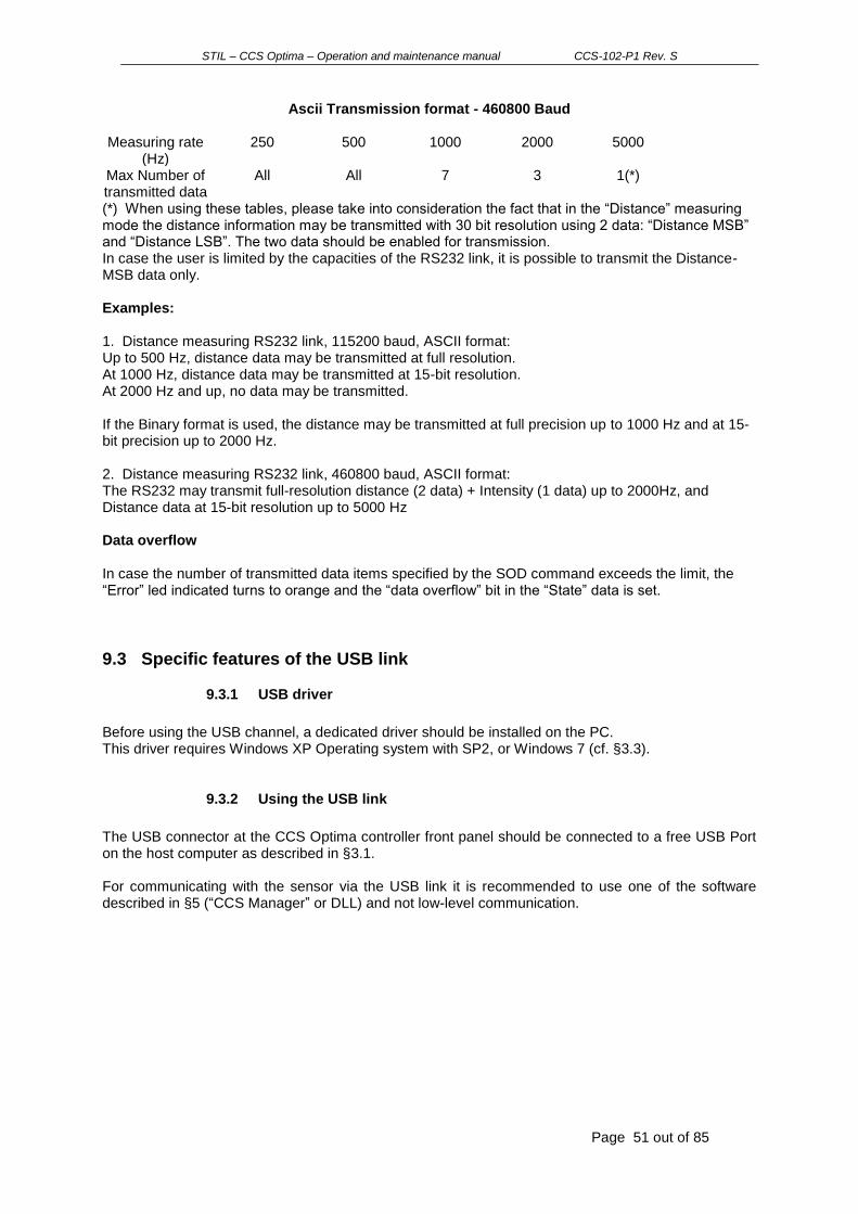
STIL – CCS Optima – Operation and maintenance manual CCS-102-P1 Rev. S
Page 51 out of 85
Ascii Transmission format - 460800 Baud Measuring rate
(Hz) 250 500 1000 2000 5000
Max Number of transmitted data
All All 7 3 1(*)
(*) When using these tables, please take into consideration the fact that in the “Distance” measuring mode the distance information may be transmitted with 30 bit resolution using 2 data: “Distance MSB” and “Distance LSB”. The two data should be enabled for transmission. In case the user is limited by the capacities of the RS232 link, it is possible to transmit the Distance-MSB data only. Examples: 1. Distance measuring RS232 link, 115200 baud, ASCII format: Up to 500 Hz, distance data may be transmitted at full resolution. At 1000 Hz, distance data may be transmitted at 15-bit resolution. At 2000 Hz and up, no data may be transmitted. If the Binary format is used, the distance may be transmitted at full precision up to 1000 Hz and at 15-bit precision up to 2000 Hz. 2. Distance measuring RS232 link, 460800 baud, ASCII format: The RS232 may transmit full-resolution distance (2 data) + Intensity (1 data) up to 2000Hz, and Distance data at 15-bit resolution up to 5000 Hz Data overflow In case the number of transmitted data items specified by the SOD command exceeds the limit, the “Error” led indicated turns to orange and the “data overflow” bit in the “State” data is set.
9.3 Specific features of the USB link
9.3.1 USB driver
Before using the USB channel, a dedicated driver should be installed on the PC. This driver requires Windows XP Operating system with SP2, or Windows 7 (cf. §3.3).
9.3.2 Using the USB link
The USB connector at the CCS Optima controller front panel should be connected to a free USB Port on the host computer as described in §3.1. For communicating with the sensor via the USB link it is recommended to use one of the software described in §5 (“CCS Manager” or DLL) and not low-level communication.
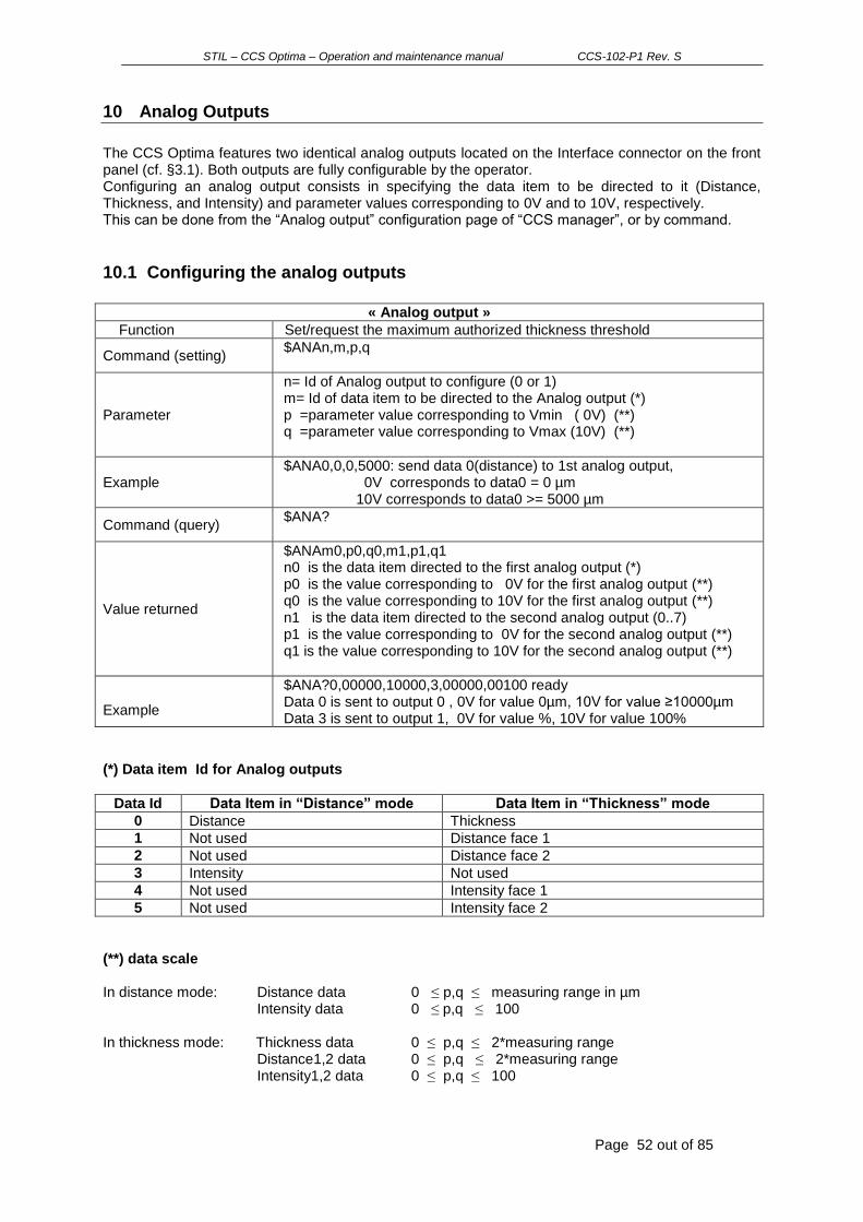
STIL – CCS Optima – Operation and maintenance manual CCS-102-P1 Rev. S
Page 52 out of 85
10 Analog Outputs
The CCS Optima features two identical analog outputs located on the Interface connector on the front panel (cf. §3.1). Both outputs are fully configurable by the operator. Configuring an analog output consists in specifying the data item to be directed to it (Distance, Thickness, and Intensity) and parameter values corresponding to 0V and to 10V, respectively. This can be done from the “Analog output” configuration page of “CCS manager”, or by command.
10.1 Configuring the analog outputs
« Analog output »
Function Set/request the maximum authorized thickness threshold
Command (setting) $ANAn,m,p,q
Parameter
n= Id of Analog output to configure (0 or 1) m= Id of data item to be directed to the Analog output (*) p =parameter value corresponding to Vmin ( 0V) (**) q =parameter value corresponding to Vmax (10V) (**)
Example $ANA0,0,0,5000: send data 0(distance) to 1st analog output, 0V corresponds to data0 = 0 µm 10V corresponds to data0 >= 5000 µm
Command (query) $ANA?
Value returned
$ANAm0,p0,q0,m1,p1,q1 n0 is the data item directed to the first analog output (*) p0 is the value corresponding to 0V for the first analog output (**) q0 is the value corresponding to 10V for the first analog output (**) n1 is the data item directed to the second analog output (0..7) p1 is the value corresponding to 0V for the second analog output (**) q1 is the value corresponding to 10V for the second analog output (**)
Example
$ANA?0,00000,10000,3,00000,00100 ready Data 0 is sent to output 0 , 0V for value 0µm, 10V for value ≥10000µm Data 3 is sent to output 1, 0V for value %, 10V for value 100%
(*) Data item Id for Analog outputs
Data Id Data Item in “Distance” mode Data Item in “Thickness” mode
0 Distance Thickness
1 Not used Distance face 1
2 Not used Distance face 2
3 Intensity Not used
4 Not used Intensity face 1
5 Not used Intensity face 2
(**) data scale In distance mode: Distance data 0 ≤ p,q ≤ measuring range in µm Intensity data 0 ≤ p,q ≤ 100 In thickness mode: Thickness data 0 ≤ p,q ≤ 2*measuring range Distance1,2 data 0 ≤ p,q ≤ 2*measuring range Intensity1,2 data 0 ≤ p,q ≤ 100

STIL – CCS Optima – Operation and maintenance manual CCS-102-P1 Rev. S
Page 53 out of 85
Notes: (1) The parameter p (0V value) may be smaller or larger than the parameter q (10V).
If p<q the output voltage increases when data increases, if p>q it is inversed. (2) A small constant offset (<0.2V) may be observed (“ADC offset”). To correct for this offset,
measure the actual voltage when the data value is 0, and subtract this value from all subsequent measures. The offset is the same for the 2 analog outputs and independent of the selected data.
10.2 Setting the zero values
A simplified method for configuring the Analog outputs is available using the “Set Zero” button on the front panel and/or the SOF command. This method may be used to set the 0V-level of both analog outputs to the current value of the data directed to them.
« Set Analog output Zero »
Function Set/reset the analog output 0V value
Command (setting) SOFn
Parameter
b=0/1 0: set 0V values to current values (equivalent to “Set Zero” button) 1: reset 0V values to 0 (cancels “Set Zero” button operation)
Example SOF1 (reset 0V values)
Command (query) Not available
Note: - The “Set Zero” button has no effect on the 10V values. - This button does not affect the “ADC offset”.
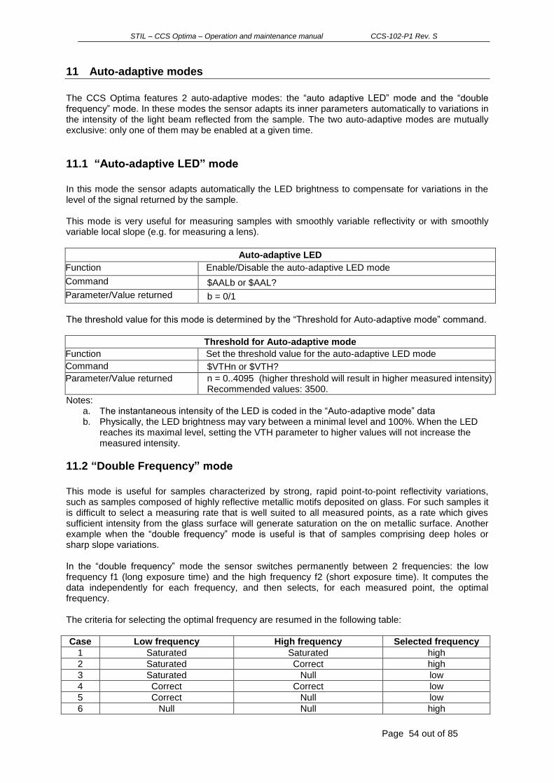
STIL – CCS Optima – Operation and maintenance manual CCS-102-P1 Rev. S
Page 54 out of 85
11 Auto-adaptive modes
The CCS Optima features 2 auto-adaptive modes: the “auto adaptive LED” mode and the “double frequency” mode. In these modes the sensor adapts its inner parameters automatically to variations in the intensity of the light beam reflected from the sample. The two auto-adaptive modes are mutually exclusive: only one of them may be enabled at a given time.
11.1 “Auto-adaptive LED” mode
In this mode the sensor adapts automatically the LED brightness to compensate for variations in the level of the signal returned by the sample. This mode is very useful for measuring samples with smoothly variable reflectivity or with smoothly variable local slope (e.g. for measuring a lens).
Auto-adaptive LED
Function Enable/Disable the auto-adaptive LED mode
Command $AALb or $AAL?
Parameter/Value returned b = 0/1
The threshold value for this mode is determined by the “Threshold for Auto-adaptive mode” command.
Threshold for Auto-adaptive mode
Function Set the threshold value for the auto-adaptive LED mode
Command $VTHn or $VTH?
Parameter/Value returned n = 0..4095 (higher threshold will result in higher measured intensity) Recommended values: 3500.
Notes: a. The instantaneous intensity of the LED is coded in the “Auto-adaptive mode” data b. Physically, the LED brightness may vary between a minimal level and 100%. When the LED
reaches its maximal level, setting the VTH parameter to higher values will not increase the measured intensity.
11.2 “Double Frequency” mode
This mode is useful for samples characterized by strong, rapid point-to-point reflectivity variations, such as samples composed of highly reflective metallic motifs deposited on glass. For such samples it is difficult to select a measuring rate that is well suited to all measured points, as a rate which gives sufficient intensity from the glass surface will generate saturation on the on metallic surface. Another example when the “double frequency” mode is useful is that of samples comprising deep holes or sharp slope variations. In the “double frequency” mode the sensor switches permanently between 2 frequencies: the low frequency f1 (long exposure time) and the high frequency f2 (short exposure time). It computes the data independently for each frequency, and then selects, for each measured point, the optimal frequency. The criteria for selecting the optimal frequency are resumed in the following table:
Case Low frequency High frequency Selected frequency
1 Saturated Saturated high
2 Saturated Correct high
3 Saturated Null low
4 Correct Correct low
5 Correct Null low
6 Null Null high

STIL – CCS Optima – Operation and maintenance manual CCS-102-P1 Rev. S
Page 55 out of 85
Each couple of acquisitions (one with long exposure and the other with short exposure) is called “a cycle”. The sensor delivers one “synchro out” signal per cycle. Measured data is transmitted once per cycle on the digital outputs and updated once per cycle on the analog outputs. The cycle rate fc is given by the relation:
1/fc = 1/f1 + 1/f2
11.2.1 Activation The “double frequency” mode can be activated from the “Basic” configuration page of “CCS manager” Or by the DFA command
“Double Frequency” Activation
Function Enable/Disable the double frequency mode
Command $DFAb or $DFA?
Parameter/Value returned b = 0/1 (1 to enable)
This command is not authorized when the “auto-adaptive LED” or the “auto-adaptive dark” modes are active (the query form “DFA?” Is authorized).
11.2.2 Frequencies The DFF command sets (or requests) the 2 frequencies for the mode
“Double Frequency” frequencies
Function Set/Request the 2 frequencies for the “double frequency” mode
Command $DFFf1,f2 or $DFF?
Parameter/Value returned f1 = low frequency, f2= high frequency in Hz conditions: frm ≤ f1 < f2 ≤ 10000 Hz,
where frm is the min authorized rate of the sensor
11.2.3 Intensity
The intensity measured by the sensor depends, on one hand, on the characteristics of the sample (reflectivity, slope) and on the other, on the exposure time. In standard operation mode (“single frequency”) the exposure time is constant so that observed intensity variations are directly related to the intensity of reflected from the sample. In the “double frequency” mode both factors vary at the same time so that the interpretation of the Intensity data may be difficult. For this reason a new parameter, the “normalized intensity” is computed. This is an intensity computed for a fixed frequency (the high frequency), so that it is directly related to the sample characteristics. Let : - ILF be the intensity measured for the low frequency - IHF be the intensity measured for the high frequency The following table shows the difference between the “raw” (standard) intensity and the “normalized” intensity.

STIL – CCS Optima – Operation and maintenance manual CCS-102-P1 Rev. S
Page 56 out of 85
Available intensities in « Double Frequency » mode
Selected Frequency
« Raw » Intensity « Normalized » Intensity
Low (f1) ILF ILF *f1/f2
High (f2) IHF IHF
By default, the transmitted Intensity data is the “Normalized” one. This option may be modified from the “Basic” configuration page of “CCS Manager”, or using the “DFI” command.
“Double Frequency” Intensity
Function Select the type of transmitted Intensity
Command $DFIb or $DFA?
Parameter/Value returned b = 0 for “Normalized” intensity, 1 for “Raw” Intensity
11.2.4 Selected frequency bit The selected frequency for a given cycle is indicated in bit 8 of the “State” data (cf. §13.7.2). 0 indicates that the high frequency was selected, 1 that that low frequency was selected.
11.2.5 Compatibility with other commands/modes The mode is compatible with most other commands and modes, and in particular: triggering, averaging and manual setting of the LED brightness. It is not compatible with: auto-adaptive LED mode, auto-adaptive dark mode, fast dark.
Command Response when the sensor is in “double frequency” mode
AAL, FDK Not authorized
DRK Authorized
TRG, TRE, TRN, TRS, TRF Authorized
AVR, HLV Authorized
LED Authorized
FRQ, TEX, SRA Authorized (the rate/exposure time is memorized. It is applied when the sensor quits the double frequency mode)
Note for users familiar with previous versions of the CCS Sensor firmware: The “selected frequency” bit replaces the “trigger flip flop” bit of previous versions.
STIL – CCS Optima – Operation and maintenance manual CCS-102-P1 Rev. S
Page 57 out of 85
11.2.6 Intensity LED indicator in “Double Frequency” mode In the “Double Frequency” mode the “Intensity” LED indicator on the front panel is correlated to the High Frequency:
- If it is red the signal is saturated at both frequency: you must lower the LED intensity or increase f2.
- If it is green, measurement is OK - If it is yellow, it should be ignored.
11.2.7 Synchronization in “double frequency” mode This paragraph is relevant for applications where the sensor is synchronized with external devices as a “master”, using the “Sync out” TTL signals, and the sensor is configured to double-frequency mode. In single-frequency mode these signals are emitted at the middle of the exposure cycle. As an example, with no averaging the exposure cycle is simple the exposure of a single frame, so that the “sync out” pulses are emitted in the middle of the exposure time of each individual frame. With averaging of 4, the acquisition cycle consists of the exposure of 4 frames, and the “sync out” pulses are emitted just between the end of exposure of the second frame and the beginning of the exposure of the third frame of the cycle. If the sample is moving, the instant these signals are emitted corresponds to the average position of the sample during the exposure. In double-frequency mode there are two exposures, one of which is used and the other one abandoned. During the exposure the sensor does not “know” yet which exposure will be selected: the decision is taken only after both images have been read and processed. For this reason the “sync out” pulses are always sent at the middle of the “short” exposure (high rate). If the short exposure is selected, there is no need for correction. If the long exposure is selected, the
“sync out” is shifted by t relative to the exact instant where they should have been emitted. Suppose now that these pulses are used to latch (read) the position of an encoder and that the sample moves
at a velocity V. The temporal shift generates a position shift x between the position latched from the encoder and the “real” position at the middle of the “long” exposure:
t = - 0.5 * fc
x =V * t Where fc is the cycle frequency given by the relation: 1/fc = 1/f1 + 1/f2 In some applications it is desirable to compensate for this shift. As an example consider the application where the depth, width and slope of a scratch on the surface of a flat surface should be measured. Double frequency may be required for this application as the intensity from the slope and/or from the bottom of the scratch is very low, while the intensity from the flat surface is very high. The depth is derived from the difference of the distance values measured on the surface and on the bottom – this data is exact, there is no need for any correction. However the width and the slope involve both sensor data and position data, so that correction should be applied to the position data by post-processing. The “selected frequency” bit in the “State” data may be used for this purpose: { 0 if “selected frequency bit”=0 Correction = {
{ V *t if “selected frequency bit”=1. If the sample is scanned back and forth please note that the sample velocity V is a signed quantity.

STIL – CCS Optima – Operation and maintenance manual CCS-102-P1 Rev. S
Page 58 out of 85
12 Synchronization
It is often necessary to synchronize the sensor with an external device, such as an encoder, a motion controller or a photocell indicating the approach of an object traveling on a conveyor belt. When the external device to be synchronized with the sensor is a digital encoder, this task is particularly easy, as it is performed automatically by the CCS Optima. All you need to do is
Connect the encoders to the “Encoder connector” on the front panel as described in §3.1.6,
Reset each encoder by positioning it at the origin point of the motion range and sending the “Reset Encoder” (“$RCD”) command,
Configure the sensor to transmit encoder data as well as data measured by the CCS Optima This may be done either from the “Encoder” page of “CCS Manager” or using the “$SOD” command (cf. §9.1)
For other types of devices (analog encoders, motion controllers) synchronization may be achieved using synchronization signals and Trigger modes. The CCS Optima may be synchronized with an external device as “master” (using the “Sync out” TTL signals), as a “slave” (using the “Sync in” TTL signals), or in a mixed mode (using both types of signals). “Trigger modes” specify the way the sensor should respond to rising or falling edges of the “Sync in” signals. The common feature to all trigger modes is that the sensor stops measuring and stands by for an “active” edge on “Sync in” connector. Trigger modes may be enabled and disabled from the “Trigger” page of the “CCS manager” program, by the DLL or by low-level commands. By default, all trigger modes are disabled, and the sensor transmits data without interruption immediately after startup. When no trigger mode is enabled, rising and falling edges of the “Sync in” signal are simply ignored.
12.1 “Sync out” signals
Synchronizing the sensor as a “master” means that the “Sync out” TTL signals emitted by the sensor are used to trig (latch) the external device. The sensor emits one “Sync out” pulse for each measured point at the middle of the Cycle Exposure Time (CET).
CET = EET * AVR Where EET = Elementary Exposure Time = 1/measuring rate, AVR = averaging factor. Example: for a measuring rate of 100 Hz, the Elementary Exposure Time is 10 ms. By default, the sensor measures with no averaging (AVR=1), so that the Cycle Exposure Time equals the Elementary Exposure Time. If the sensor is configured to an averaging factor of 5, the CET equals 50 ms, as 5 frames are acquired and averaged for each measured point. In the case of double-frequency rate, please refer to §11.3.7 The duration of the “Sync out” pulse (high state) is 10 µs, irrespective of the CET. “Sync out” pulses are emitted automatically, with no need for any special configuration. When the sensor is in stand-by for a trigger, no “sync out” pulses are emitted.
12.1.1 Sampling of syncout pulses:
In some application one wishes to reduce the rate of syncout pulses while keeping the data rate. This may happen when there is a limitation on the rate of latching an encoder or a motion controller. The TRO command allows modifying this parameter

STIL – CCS Optima – Operation and maintenance manual CCS-102-P1 Rev. S
Page 59 out of 85
Sampling trigger-out pulses
Function Reduces sync out pulse rate (1 per n measurements)
Command $TROn or $TRO ?
Parameter/Value returned Fixes or inquires for the sync-out sampling (default = 1).
12.2 “Sync in” signals
Synchronizing the sensor as a “slave” means that the sensor stands by for a trigger signal from the external device. So long as no trigger signal arrives, the sensor is “silent”: it does not transmit any data and does not emit any “Sync out” pulse. As soon as it detects a trigger signal on the “Sync in” connector, the sensor starts measuring and emitting “Sync out” pulses. The “Sync in” signals are 0V-5V TTL signals generated by external devices and intercepted by the sensor. The “active” edge of the « Sync in » signal is the edge which triggers measurement. The active edge (rising edge or falling edge) may be selected by command. The duration of the « Sync in » pulses should be at least 1.2 µs.
12.3 Trigger modes
The simplest trigger mode is the “Start on edge” trigger. It is enabled by sending the “$TRG” command, either from the Command Terminal or from the “Trigger” page of the “CCS Manager” program. On receipt of the command, the sensor stands by for the trigger signal. Measurement starts as soon as an “active” edge is detected at the "Sync in" input, with repeatability (jitter) better than 1 µs. Once the first "Sync in" pulse is received, the sensor exits the “Start on edge” Trigger mode and resumes normal operation. Additional "Sync in" pulses are simply ignored. Besides the “Start” trigger mode described above, the sensor offers 4 additional trigger modes:
In the “Start/Stop on State” trigger mode, data transmission starts and stops according to the state of the "Sync in" signal. As an example, data transmission starts when the "Sync in" signal is high (5V) and stops when it is low (0V).
The “Start/Stop on Edge” trigger mode is similar to the “Start/Stop on State”, with one difference: data transmission starts and stops by successive "Sync in" pulses and not by changes in signal state.
In the “Burst” trigger mode, the sensor “latches” (transmits) the data of a preset number of points each time it receives a "Sync in" pulse.
In the “Stop” trigger mode the sensor is disabled. Soft and hard triggers are ignored. Unlike the “Start” trigger mode which is disabled automatically by the first “Sync in” pulse received, the “Start/Stop on State”, “Start/Stop on edge” and “Burst” trigger modes should be explicitly disabled by commands. As long as these trigger modes are enabled, successive “Sync in” pulses keep triggering measurements. When all trigger modes are disabled, the sensor resumes normal operation and

STIL – CCS Optima – Operation and maintenance manual CCS-102-P1 Rev. S
Page 60 out of 85
additional “Sync in” pulses are ignored. The table next page resumes sensor behavior in the different trigger modes
Notes:
The emission of “Sync out” signals stops and restarts together with data transmission.
Each time the sensor starts measuring after a stand-by period, the counter is reset.
12.4 Trigger configuration
12.4.1 “Start” (“TRG”) trigger
The « Start Trigger » command puts the sensor on standby for a trigger signal. As soon as an active edge is detected at the "Sync in" input, the sensor starts measuring. Additional “Sync in” signals are ignored.
“Start” trigger
Function Enable “Start” trigger mode.
Command $TRG
Parameter/Value returned None
To disable this mode without a hardware trigger, send a “$STR” (software trigger) command, and the sensor starts measuring again.
12.4.2 “Start/stop on state” (“TRN”) trigger
Data is transmitted when the “Sync in” signal is at the active state. The Active state (high or low) is determined by the “TRF” command.
“Start/stop on state” trigger
Function Enable/Disable the “Start/Stop on State” trigger
Command $TRNb
Parameter/Value returned b=1/0
The software trigger does not work in this mode.
Active trigger mode Response to active “Sync in” edges
Response to inactive “Sync in” signal edges
“Start” 1st active edge starts measurement
Next ones are ignored
Ignored
“Start/Stop on State” Start measurement Stop measurement
“Start/Stop on Edge” 1st active edge starts measurement,
2nd
active edge stops measurement,
3rd
active edge starts measurement, And so forth.
ignored
“Burst” Measure a pre-fixed number of points (N) Ignored
“Stop” Ignored Ignored
None Ignored Ignored
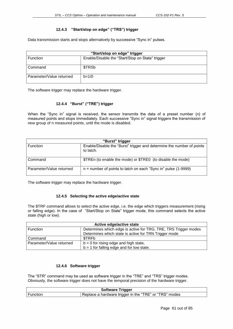
STIL – CCS Optima – Operation and maintenance manual CCS-102-P1 Rev. S
Page 61 out of 85
12.4.3 “Start/stop on edge” (“TRS”) trigger
Data transmission starts and stops alternatively by successive “Sync in” pulses.
“Start/stop on edge” trigger
Function Enable/Disable the “Start/Stop on State” trigger
Command $TRSb
Parameter/Value returned b=1/0
The software trigger may replace the hardware trigger.
12.4.4 “Burst” (“TRE”) trigger
When the “Sync in” signal is received, the sensor transmits the data of a preset number (n) of measured points and stops immediately. Each successive “Sync in” signal triggers the transmission of new group of n measured points, until the mode is disabled.
“Burst” trigger
Function Enable/Disable the “Burst” trigger and determine the number of points to latch.
Command $TREn (to enable the mode) or $TRE0 (to disable the mode)
Parameter/Value returned n = number of points to latch on each “Sync in” pulse (1-9999)
The software trigger may replace the hardware trigger.
12.4.5 Selecting the active edge/active state
The $TRF command allows to select the active edge, i.e. the edge which triggers measurement (rising or falling edge). In the case of “Start/Stop on State” trigger mode, this command selects the active state (high or low).
Active edge/active state
Function Determines which edge is active for TRG, TRE, TRS Trigger modes Determines which state is active for TRN Trigger mode
Command $TRFb
Parameter/Value returned b = 0 for rising edge and high state, b = 1 for falling edge and for low state.
12.4.6 Software trigger
The “STR” command may be used as software trigger in the “TRE” and “TRS” trigger modes. Obviously, the software trigger does not have the temporal precision of the hardware trigger.
Software Trigger
Function Replace a hardware trigger in the “TRE” or “TRS” modes

STIL – CCS Optima – Operation and maintenance manual CCS-102-P1 Rev. S
Page 62 out of 85
Command $STR
Parameter/Value returned None
Trouble shooting:
(1) The Command Terminal of the “CCS Manager” command does not handle the “STR” command correctly.
(2) In RS232 communication, the $ sign acts as a software trigger in “TRG” mode. You may use
Other trigger modes if you wish to send commands by RS232 while the sensor is in standny for trigger.
(3) The software trigger is not available in the “TRN” mode since it simulates a pulse, not a state.
If you wish to use software trigger, use the “TRS” mode instead.
12.4.7 “Stop” trigger mode
The “STP” command is a comfortable means to start and stop measuring using software command.
This mode resembles to TRS mode, however when standing by for “STP0” command the sensor will not react to hardware trigger.
“Stop” trigger mode
Function Start/stop measuring by command
Command $STP1 : the sensor stops measuring $STP0: the sensor resumes measuring
12.5 Identification of the first point measured after trigger
When operating in triggered mode the sensor starts and stops measuring according to the state of the “Sync out” signal. This signal is usually generated by an external device, it arrives to the sensor and not to the user program running on the PC. Except in the case of the “burst” trigger, the user program does not “know” how many points are measured during each time the trigger is “open”. As an example consider a case of a sensor located above a conveyor belt. The sensor is configured to the “Start/Stop on state” mode and the “Sync in” signal, generated by an optical sensor, is high whenever a product is present inside the sensor‟s field of view. The user program has to process the data profiles and identify the products which do not comply with certain specifications. This program uses one or more large buffers for accumulating the sensor data. The first difficulty that this program has to face is the identification of the limits of each profile, in other words, the identification of the data corresponding to the first point measured after the “sync in” signal goes from low to high. The solution to this problem resides in the “Counter” data: the counter is reset each time the sensor starts measuring after standby, for all trigger modes. By configuring the sensor to transmit this data together with the “Distance” and the “Intensity” data the user program can easily detect the limits of each profile.
12.6 Maximum rate of “Sync in” pulses
The maximum rate of the “Sync in” pulses is limited by the cycle time required for the exposure, signal reading, data computation and data transmission.
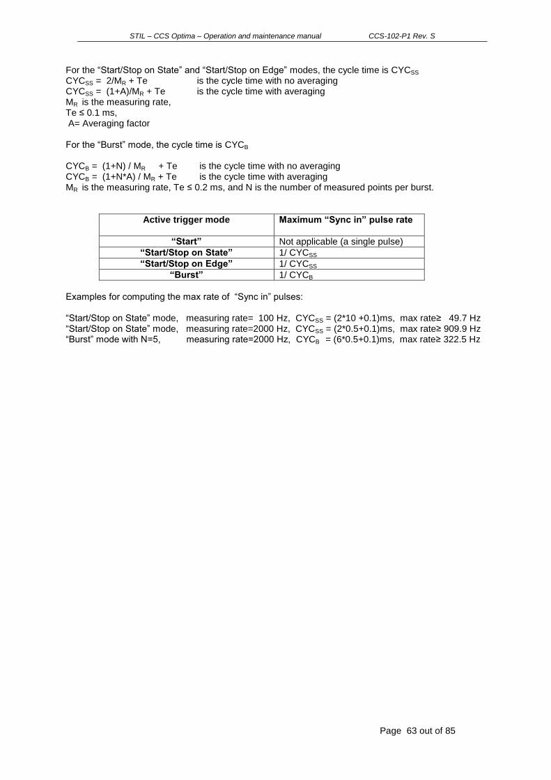
STIL – CCS Optima – Operation and maintenance manual CCS-102-P1 Rev. S
Page 63 out of 85
For the “Start/Stop on State” and “Start/Stop on Edge” modes, the cycle time is CYCSS CYCSS = 2/MR + Te is the cycle time with no averaging CYCSS = (1+A)/MR + Te is the cycle time with averaging MR is the measuring rate, Te ≤ 0.1 ms, A= Averaging factor For the “Burst” mode, the cycle time is CYCB CYCB = (1+N) / MR + Te is the cycle time with no averaging CYCB = (1+N*A) / MR + Te is the cycle time with averaging MR is the measuring rate, Te ≤ 0.2 ms, and N is the number of measured points per burst.
Active trigger mode Maximum “Sync in” pulse rate
“Start” Not applicable (a single pulse)
“Start/Stop on State” 1/ CYCSS
“Start/Stop on Edge” 1/ CYCSS
“Burst” 1/ CYCB
Examples for computing the max rate of “Sync in” pulses: “Start/Stop on State” mode, measuring rate= 100 Hz, CYCSS = (2*10 +0.1)ms, max rate≥ 49.7 Hz “Start/Stop on State” mode, measuring rate=2000 Hz, CYCSS = (2*0.5+0.1)ms, max rate≥ 909.9 Hz “Burst” mode with N=5, measuring rate=2000 Hz, CYCB = (6*0.5+0.1)ms, max rate≥ 322.5 Hz
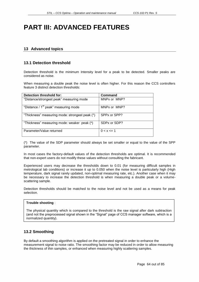
STIL – CCS Optima – Operation and maintenance manual CCS-102-P1 Rev. S
Page 64 out of 85
PART III: ADVANCED FEATURES 13 Advanced topics
13.1 Detection threshold
Detection threshold is the minimum Intensity level for a peak to be detected. Smaller peaks are considered as noise. When measuring a double peak the noise level is often higher. For this reason the CCS controllers feature 3 distinct detection thresholds:
Detection threshold for: Command
“Distance/strongest peak” measuring mode MNPx or MNP?
“Distance / 1st peak” measuring mode
MNPx or MNP?
“Thickness” measuring mode: strongest peak (*) SPPx or SPP?
“Thickness” measuring mode: weaker peak (*) SDPx or SDP?
Parameter/Value returned 0 < x <= 1
(*) The value of the SDP parameter should always be set smaller or equal to the value of the SPP parameter. In most cases the factory-default values of the detection thresholds are optimal. It is recommended that non-expert users do not modify these values without consulting the fabricant.
Experienced users may decrease the thresholds down to 0.01 (for measuring difficult samples in metrological lab conditions) or increase it up to 0.050 when the noise level is particularly high (High temperature, dark signal rarely updated, non-optimal measuring rate, etc.). Another case when it may be necessary to increase the detection threshold is when measuring a double peak or a volume-scattering sample.
Detection thresholds should be matched to the noise level and not be used as a means for peak selection.
13.2 Smoothing
By default a smoothing algorithm is applied on the pretreated signal in order to enhance the measurement signal to noise ratio. The smoothing factor may be reduced in order to allow measuring the thickness of thin samples, or enhanced when measuring highly scattering samples.
Trouble shooting : The physical quantity which is compared to the threshold is the raw signal after dark subtraction (and not the preprocessed signal shown in the “Signal” page of CCS manager software, which is a normalized quantity).

STIL – CCS Optima – Operation and maintenance manual CCS-102-P1 Rev. S
Page 65 out of 85
Smoothing (CCI)
Function Set/Get the smoothing factor
Command $SLIn or $SLI?
Parameter/Value returned n=0/1/2/4 default value=2.
13.3 “First peak” mode
“First peak” mode is a feature of the “Distance” measuring mode that is useful for samples comprising one or more transparent layers, e.g. samples whose surface is partially covered with a transparent coating. In this case the sensor “sees” 2 peaks, one from the outer coating surface and one from the substrate. For such samples the reflection of the surface beneath the coating may be stronger than that from the outer coating surface. In order that the sensor detect the first peak (instead of the strongest peak, which it does by default), the “First peak” mode should be enabled. In this mode the sensor selects the first peak that is higher than the detection threshold.
“First peak” mode
Function Enable/Disable the “First peak” mode
Command $MSPb or $MSP?
Parameter/Value returned b = 0 (Strongest peak) or 1 (First Peak).
Notes:
(1) In the “Thickness” measuring mode this command has no effect. (2) The detection threshold in this mode is determined by the MNP command. (3) This mode is very sensitive to noise. In case of false detection of noise peak:
- update the dark signal measurement and increase the threshold.
13.4 “Altitude” mode
“Altitude” mode is a feature of the “Distance” measuring mode. When this mode is enabled, the Distance scale is reversed (Altitude instead of Distance): In Distance mode, Altitude is computed as:
Altitude=Measuring range –Distance
In Thickness mode, the effective measuring range is n*measuring range in air (n is the refractive index), so that Distance2 may be greater than the measuring range. To avoid negative values, the Altitudes are computed as: Altitude1= 2*Measuring Range – Distance1 Altitude1= 2*Measuring Range – Distance2 Note that this means that the Altitude origin is not the same for Distance mode and for Thickness mode.
“Altitude” mode
Function Enable/Disable the “Altitude” mode
Command $RVSb or $RVS?
Parameter/Value returned b = 0 (Distance) or 1 (Altitude).

STIL – CCS Optima – Operation and maintenance manual CCS-102-P1 Rev. S
Page 66 out of 85
13.5 Handling of unmeasured peak in Thickness mode
It may happen a single peak is detected while the sensor is configured to “Thickness” mode; this may occur if one of the other of the sample faces is outside the measuring range, or if one of the signals is too weak. The “Unmeasured peak handling” command determines the behavior of the sensor in such a case: Option 1 (default) - set Distance1, Intensity1 and Barycenter1 to measured values of the single peak - set Distance2, Intensity2 and Barycenter2 equal to Distance1, Intensity1 and Barycenter1, respectively - set the thickness to 0 Option 2: - set Distance1, Intensity1 and Barycenter1 to measured values of the single peak - set Distance2, Intensity2 and Barycenter2 to 0 - set the thickness to 0
“Unmeasured peak handling” in Thickness mode
Function Determine the values of Distance2, Intensity2 and Barycenter2 data in case a single peak is detected while the sensor is in “Thickness” mode
Command $RSPb or $RSP?
Parameter/Value returned b = 0 (Option 2 above) or 1 (option 1 above).
13.6 Watchdog
The sensor features software “Watchdog”, i.e. a permanent test that validates that the sensor operates normally. In case it does not, the Watchdog resets the sensor after 40 seconds. This feature is useful for the case the sensor is blocked due to an incomplete command or another reason, in particular for sensors that are not easily accessible. It may be disabled and enabled with the “Watch dog” command.
Watchdog activation
Function Enable/Disable the watchdog
Command $WDEb or $WDE?
Parameter/Value returned b = 0 /1
13.7 “Counter”, “State” and “Auto-adaptive mode” data
Besides measured data (Distance, Intensity, Barycenter) the sensor also delivers 3 data for controlling the sensor state and for facilitating its integration. These data may be sent on the digital output at the same time as measured data, using the SOD command or any of the software described in §5.
13.7.1 The “Counter” data
The “Counter” data is an aid for software developers who wish to check that there is no data loss in their acquisition software.

STIL – CCS Optima – Operation and maintenance manual CCS-102-P1 Rev. S
Page 67 out of 85
The 15-bit counter is reset each time a Trigger signal is received when the sensor is one of the trigger modes: TRE, TRN, TRS or TRG.
13.7.2 The “State” data
The “State” data is an aggregate of various flags.
bit flag bit flag
0 HLV Barycentre face 2 8 Selected frequency (DF mode) (*)
1 HLV Barycentre face 1 9 reserved
2 HLV Distance face 2 10 Data overflow for RS transmission
3 HLV Distance face 1 11
4 HLV Thickness 12
5 HLV intensity face 2 13
6 HLV Intensity face 1 14
7 Saturation flag 15
The HLV bits are set if the corresponding data is not measured but “held” at last valid value in “Hold last value” mode. Saturation flag indicates signal saturation. It is set at the same time the “Intensity” LED indicator color turns to red. The “selected frequency” flag is significant on double-frequency mode only. 0 indicates that the high frequency was selected, 1 that the low frequency was selected. (*) Note: This bit replaces the “Trigger Flip-flop” bit of previous versions. (The “Trigger Flip Flop” bit was redundant with the “Counter” data). The “data overflow” flag indicates that the number of transmitted data directed to the RS232/RS422 port exceeds the max number of transmissible data (cf. § 9.2). Note that this bit is set at the same time as the “Error” LED-indicator turns Orange.
13.7.3 The “Auto-adaptive mode” data
In the “Auto-adaptive LED” mode, this data contains the instantaneous LED brightness coded over 8 bits (0..255). This may be useful for analyzing the relative intensity of the signal returned from the sample, as in this mode the “Intensity” data is practically constant. Relative Intensity = measured Intensity / n. n = Auto adaptive mode data value

STIL – CCS Optima – Operation and maintenance manual CCS-102-P1 Rev. S
Page 68 out of 85
14 Low-level Commands
If you use « CCS Manager » or the DLL for configuring the sensor, you may skip this chapter.
14.1 Command Language
Command language is the same for the two digital I/O channels. The command language syntax is almost identical for all STIL point sensor controllers (CHR150, CCS Optima, STIL-Initial, STIL-Duo). The basic commands are common to all controllers; however, each controller has some specific commands.
14.1.1 Command syntax
(*) Actually if the sensor receives the exact number of digits it waits for, the termination sequence is not required. Example: no sequence is required after $AVR0001. However, if you send $AVR1 the sensor will stand by for the next digits and will not respond, unless a termination sequence is received. In order to avoid confusion, we recomand sending the termination sequence after each commands comprising parameters. (**) For common Terminal applications such as windows
TM HyperTerminal
TM the order of the two
characters has no importance.
14.1.2 Sensor response When powered on, the sensor transmits data according to the last saved configuration. On receipt of character $, the sensor stops sending data and waits for the remaining command characters. Each received character (including $) is echoed back. After processing the command, the sensor responds with one of the following strings, and switches back to normal operation.
Every command transmitted to the sensor must start by a $ character.
Every command must end with a termination sequence (*)
For CCS, STIL-Duo and STIL-Initial the termination sequence is <LFCR> (line feed, carriage return). For CHR150, the termination sequence is <CRLF> (carriage return, line feed).(**)
Command name consists of 3 higher case letters.
When a command has one or more parameters, the parameters come immediately after the command name.
There should be no comma between the name of the command and the first parameter.
When a command includes several parameters, the parameters are separated by commas.
For query the parameter is replaced by “?”
Note: in USB communication, the entire command should be sent as a single packet.
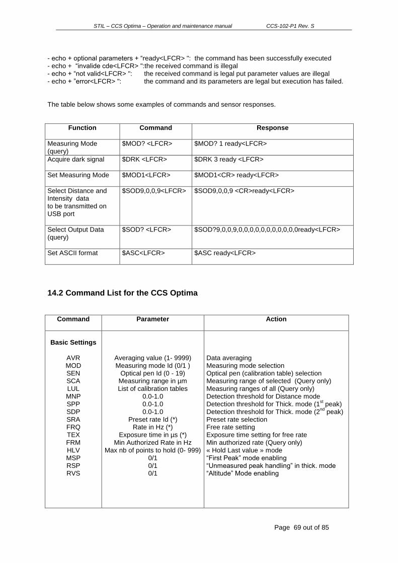
STIL – CCS Optima – Operation and maintenance manual CCS-102-P1 Rev. S
Page 69 out of 85
- echo + optional parameters + “ready<LFCR> ": the command has been successfully executed - echo + “invalide cde<LFCR> ":the received command is illegal - echo + “not valid<LFCR> ": the received command is legal put parameter values are illegal - echo + ”error<LFCR> ": the command and its parameters are legal but execution has failed. The table below shows some examples of commands and sensor responses.
Function Command Response
Measuring Mode (query)
$MOD? <LFCR> $MOD? 1 ready<LFCR>
Acquire dark signal $DRK <LFCR> $DRK 3 ready <LFCR>
Set Measuring Mode
$MOD1<LFCR> $MOD1<CR> ready<LFCR>
Select Distance and Intensity data to be transmitted on USB port
$SOD9,0,0,9<LFCR> $SOD9,0,0,9 <CR>ready<LFCR>
Select Output Data (query)
$SOD? <LFCR> $SOD?9,0,0,9,0,0,0,0,0,0,0,0,0,0,0ready<LFCR>
Set ASCII format
$ASC<LFCR> $ASC ready<LFCR>
14.2 Command List for the CCS Optima
Command
Parameter Action
Basic Settings
AVR MOD SEN SCA LUL MNP SPP SDP SRA FRQ TEX FRM HLV MSP RSP RVS
Averaging value (1- 9999) Measuring mode Id (0/1 )
Optical pen Id (0 - 19) Measuring range in µm List of calibration tables
0.0-1.0 0.0-1.0 0.0-1.0
Preset rate Id (*) Rate in Hz (*)
Exposure time in µs (*) Min Authorized Rate in Hz
Max nb of points to hold (0- 999) 0/1 0/1 0/1
Data averaging Measuring mode selection Optical pen (calibration table) selection Measuring range of selected (Query only) Measuring ranges of all (Query only) Detection threshold for Distance mode Detection threshold for Thick. mode (1
st peak)
Detection threshold for Thick. mode (2nd
peak) Preset rate selection Free rate setting Exposure time setting for free rate Min authorized rate (Query only) « Hold Last value » mode “First Peak” mode enabling “Unmeasured peak handling” in thick. mode “Altitude” Mode enabling
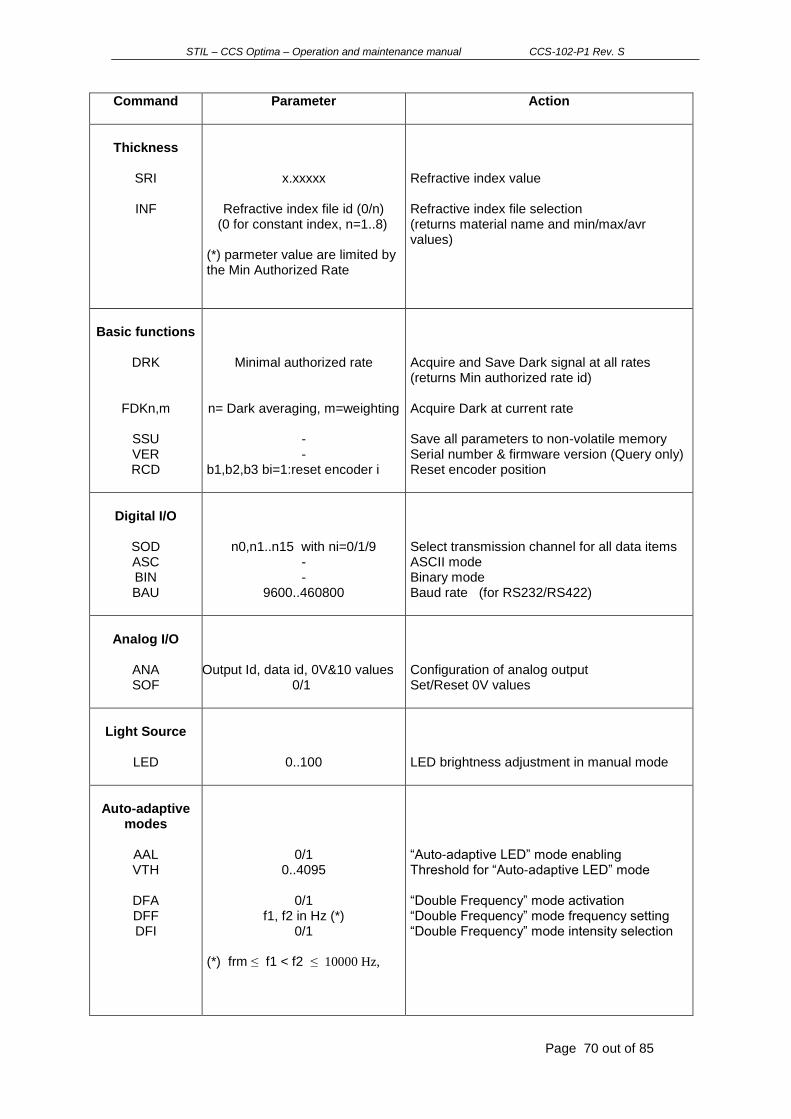
STIL – CCS Optima – Operation and maintenance manual CCS-102-P1 Rev. S
Page 70 out of 85
Command
Parameter Action
Thickness
SRI
INF
x.xxxxx
Refractive index file id (0/n) (0 for constant index, n=1..8)
(*) parmeter value are limited by the Min Authorized Rate
Refractive index value Refractive index file selection (returns material name and min/max/avr values)
Basic functions
DRK
FDKn,m
SSU VER RCD
Minimal authorized rate
n= Dark averaging, m=weighting - -
b1,b2,b3 bi=1:reset encoder i
Acquire and Save Dark signal at all rates (returns Min authorized rate id) Acquire Dark at current rate Save all parameters to non-volatile memory Serial number & firmware version (Query only) Reset encoder position
Digital I/O
SOD ASC BIN BAU
n0,n1..n15 with ni=0/1/9 - -
9600..460800
Select transmission channel for all data items ASCII mode Binary mode Baud rate (for RS232/RS422)
Analog I/O
ANA SOF
Output Id, data id, 0V&10 values
0/1
Configuration of analog output Set/Reset 0V values
Light Source
LED
0..100
LED brightness adjustment in manual mode
Auto-adaptive
modes
AAL VTH
DFA DFF DFI
0/1 0..4095
0/1
f1, f2 in Hz (*) 0/1
(*) frm ≤ f1 < f2 ≤ 10000 Hz,
“Auto-adaptive LED” mode enabling Threshold for “Auto-adaptive LED” mode “Double Frequency” mode activation “Double Frequency” mode frequency setting “Double Frequency” mode intensity selection

STIL – CCS Optima – Operation and maintenance manual CCS-102-P1 Rev. S
Page 71 out of 85
Trigger
TRG CTN TRE TRS TRN TRF
- -
0/n, n=1..9999 0/1 0/1 0/1
“Start” Trigger mode enabling “Start” Trigger mode disabling “Burst” Trigger mode enabling and setting “Start /stop on edge” Trigger mode enabling “Start/stop on state” Trigger mode enabling Select active edge
Watch dog
WDE
0/1
Watch dog enabling

STIL – CCS Optima – Operation and maintenance manual CCS-102-P1 Rev. S
Page 72 out of 85
15 DATA FORMAT AND DATA ENCODING
If you use « CCS Manager » or the DLL for acquiring the data, you may skip this chapter.
15.1 Data transmission formats
The sensor provides 2 data transmission formats: the ASCII format and the binary format. Data transmission formats are set by commands.
15.1.1 Ascii Format
Ascii
Function Configure the sensor to ASCII transmission format
Command $ASC
Parameter/Value returned None
In ASCII format, 5 characters (digits) are transmitted for each data item. The data from the same point are separated by commas, and the successive points are separated by <LFCR> sequence.
Example
Measuring mode = « Thickness », Data selected = Thickness, Distance face 1, Distance face 2. The successive measurement points are identified as A, B, C etc. The table below shows the first 36 characters transmitted:
ASCII transmission format
X X X X X , X X X X X ,
Thickness – point A DSep Distance face 1 - point A DSep
1 2 3 4 5 6 7 8 9 10 11 12
X X X X X CR LF X X X X X
Distance face 2 – point A PSep Thickness – point B
13 14 15 16 17 18 19 20 21 22 23 24
, X X X X X , X X X X X
DSep Distance face 1 – Point B DSep Distance face 2 – Point B
25 26 27 28 29 30 31 32 33 34 35 36
X = digit (0-9) DSep = Data separator (comma) PSep= Point separator (LFCR) Note that in thickness mode the distance information is provided with 15 bits resolution (one data item).

STIL – CCS Optima – Operation and maintenance manual CCS-102-P1 Rev. S
Page 73 out of 85
15.1.2 Binary format
In Binary format, 2 bytes are transmitted for each data item with no data separator. Successive points are separated by two consecutive bytes OxFF (decimal value = 255).
Binary
Function Configures the sensor to binary transmission format
Command $BIN
Parameter/Value returned None
Example
Measuring mode = « Distance », Selected data = Distance MSB and Distance LSB A,B,C = Successive measurement points. The table below shows the first 12 bytes transmitted:
Binary transmission format
X X X X OxFF OxFF X X X X OxFF OxFF
Dist – MSB Point A
Dist – LSB Point A
PSep Dist – MSB Point B
Dist – LSB Point B
PSep
1 2 3 4 5 6 7 8 9 10 11 12
X= 1 byte of data PSep = Point separator
15.2 Decoding the data
All data are encoded as integer number. The following rules allow converting them to physical quantities.
15.2.1 Data decoding for the Distance measuring mode
The Distance is encoded over 30 bits (2 data items: MSB and LSB, 15 bits each). To obtain The Distance in µm, use the following relation: The measurement range depends on the optical pen. To get the measuring range of the currently connected confocal optical pen, send the “SCA?” command.
In some cases 15-bit resolution is sufficient. In such cases a simplified relation may be used: Intensity is encoded over 12 bits (0-4095). To obtain the Intensity in % of the sensor dynamics, use the following relation:
Intensity [% ]= Transmitted Value x 100% 4095
Distance = (Transmitted value of MSB *215
+ Transmitted value of LSB)* Measurement range / 230
Distance [µm] ~ Transmitted Value of MSB x Measurement range 32767

STIL – CCS Optima – Operation and maintenance manual CCS-102-P1 Rev. S
Page 74 out of 85
The position of the Barycenter (pixel index of the spectral peak on the photodetector signal) is encoded over 15 bits (0-32767). To obtain the position of the barycenter in pixels, use the following relationship:
Encoder data is coded over 30 bits and transmitted in 2 words of 15 bits each. Value = ( ( MSB & Ox7FFF) <<15) | (LSB & Ox7FFF) The “Reset value” (2^30 / 2 = 536 870 912 = Ox2000 0000) is attributed to the position where the “$RCD” command is sent. Encoder value relative to this position = Value – Reset Value Each unit equals 1 encoder micro step. The State data is a word composed of independent bits (cf. § 13.7). The counter and the Auto-adaptive mode data are described in the “Advanced topics” chapter.
15.2.2 Data decoding for the Thickness measuring mode
In Thickness mode Distance1, Distance2 and the Thickness data are encoded over 15 bits (0-32767). As the refractive index of the sample is generally greater than 1.0, the Thickness and Distance2 may be greater than the measuring range in air. For this reason the scale is twice the measuring range in air. Note: To get the measuring range of the currently connected confocal optical pen, send the “SCA?” command. All the other data are encoded in the same way as for the CCI/Distance mode.
Thickness =Transmitted value x Measurement Range x Scale factor 32767
Distance face 1 =Transmitted value x Measurement range x Scale factor 32767
Distance face 2 =Transmitted value x Measurement range x Scale factor 32767
Scale factor =2
Barycenter = (transmitted value Bs) + Bo Bs is Barycenter scale, Bo is Barycenter offset. The default values of these parameters for the CCS Optima are:
Bs=32, Bo= 520

STIL – CCS Optima – Operation and maintenance manual CCS-102-P1 Rev. S
Page 75 out of 85
16 Maintenance
16.1 Handling the fiber optics
When no fiber optics is connected, the fiber socket located on the controller front panel must at all times be fitted with its protection cap to avoid contamination of the fiber tip, which could result in malfunctioning of the sensor. Avoid putting anything on the fiber optics or laying it on the floor (not to stamp it). Avoid wringing or bending it upwards 70 degrees
The best way to avoid contamination of the fiber optics lead is to keep it permanently connected at both ends, or if it is necessary to disconnect it, to immediately fit a protective cap on the socket at the controller front panel.
16.2 High Dark signals
The first symptom indicating the presence of dust or dirt on the fiber optics tips or inside a fiber connector is an increase in the level of the dark signal. In such a case on completion of the dark acquisition sequence the color of the blinking LED Indicators is orange or red. This means that the acquired dark signal is too high at some sampling rates (orange) or at all sampling rates (red). A high dark signal is not necessarily a problem: If you wish to measure at 2 kHz and the sensor cannot be configured to 100 Hz, there is clearly no reason to be alarmed. However if you wish to measure at 200 Hz and the sensor cannot be configured to 100 Hz, it is recommended to proceed as following: Step 1: Check that the dark signal was acquired with no object present within the measuring range. Mask the extremity of the optical pen with a piece of paper, acquire the dark signal again, and watch the color of the blinking LED Indicators at the end of the operation. If the problem persists: Step 2: Check if the problem comes from the controller or from the fiber optics connected to the optical pen. Disconnect the fiber optics from the controller front panel (do not cover the socket with the protecting cap). Acquire the dark signal, and watch the color of the blinking LED Indicators at the end of the operation. If it is orange or red, the problem comes from the fiber optics inside the controller. If it is green, the problem comes from the fiber optics connected to the optical pen. Step 3: If the problem comes from the optical pen, clean the fiber optics tip:
Note: For sensors equipped with a custom light source, the dark signal is often higher as these light sources are more intense. For such sensors the warning message should not be interpreted as an indication of a problem.

STIL – CCS Optima – Operation and maintenance manual CCS-102-P1 Rev. S
Page 76 out of 85
Raise the black protecting cap over the fiber optics plug, and clean the fiber optics tip carefully. Use absorbent cotton, or a paper towel, soaked with alcohol (e.g. Ethanol or Methanol). Perform circular movement so as to push the dust grains away from the fiber tip.
If you have tried cleaning the fiber tip once or twice and the problem persists, it means that the fiber optics is damage. In this case, replace the fiber optics cable by a new one.
Step 4: If the problem comes from the controller clean the fiber coupler inside the controller:
Turn the CCS controller OFF
Remove the 4 screws at the corners:
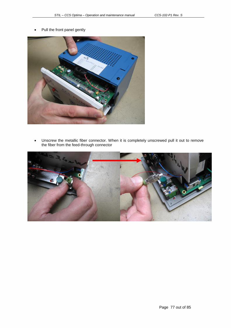
STIL – CCS Optima – Operation and maintenance manual CCS-102-P1 Rev. S
Page 77 out of 85
Pull the front panel gently
Unscrew the metallic fiber connector. When it is completely unscrewed pull it out to remove the fiber from the feed-through connector

STIL – CCS Optima – Operation and maintenance manual CCS-102-P1 Rev. S
Page 78 out of 85
Clean up the optical fiber extremity carefully with alcohol-soaked cotton :
Replace the optical fiber on the feed - through connector.
Insert carefully the front panel into the blue box.
Fasten the 4 screws.
Restart the CCS controller and launch a new a dark measurement.
16.3 Diagnostics File
The “CCS Manger” program can collect automatically the sensor configuration and generate a diagnostics file. Diagnostics file can be generated by a simple mouse click, from the “Maintenance” page of this program and saved to the computer hard disk (if your computer is connected to Internet, you may email the file directly). Whenever you contact your vendor for technical support, do not forget to join this file to your query. Note: it is recommended (but not obligatory) to generate the diagnostic files with a sample located inside the measuring range of the sensor.

STIL – CCS Optima – Operation and maintenance manual CCS-102-P1 Rev. S
Page 79 out of 85
16.4 Firmware update
The “Maintenance” page of “CCS Manager” may be also used to upload a new firmware version into the sensor. Please refer to the “Help” page describing this feature (To access help, click on the “?” mark in the menu).
16.5 Technical support
If after reading the manual you have more questions concerning the optimal way to use the sensor, please contact you vendor for technical support.
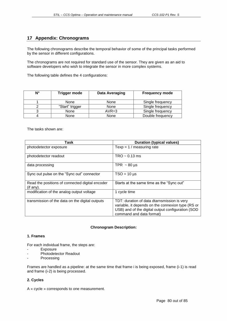
STIL – CCS Optima – Operation and maintenance manual CCS-102-P1 Rev. S
Page 80 out of 85
17 Appendix: Chronograms
The following chronograms describe the temporal behavior of some of the principal tasks performed by the sensor in different configurations. The chronograms are not required for standard use of the sensor. They are given as an aid to software developers who wish to integrate the sensor in more complex systems. The following table defines the 4 configurations:
N° Trigger mode Data Averaging Frequency mode
1 None None Single frequency
2 “Start” trigger None Single frequency
3 None AVR=3 Single frequency
4 None None Double frequency
The tasks shown are:
Task Duration (typical values)
photodetector exposure
Texp = 1 / measuring rate
photodetector readout
TRO ~ 0.13 ms
data processing
TPR ~ 80 µs
Sync out pulse on the “Sync out” connector
TSO = 10 µs
Read the positions of connected digital encoder (if any).
Starts at the same time as the “Sync out”
modification of the analog output voltage
1 cycle time
transmission of the data on the digital outputs
TDT: duration of data dtarnsmission is very variable, it depends on the connexion type (RS or USB) and of the digital output configuration (SOD command and data format)
Chronogram Description: 1. Frames For each individual frame, the steps are: - Exposure - Photodetector Readout - Processing Frames are handled as a pipeline: at the same time that frame i is being exposed, frame (i-1) is read and frame (i-2) is being processed. 2. Cycles A « cycle » corresponds to one measurement.

STIL – CCS Optima – Operation and maintenance manual CCS-102-P1 Rev. S
Page 81 out of 85
With no averaging, the cycle is a single frame (in “Single Frequency” mode) or a couple of frames, one with long exposure and one with short exposure (in “Double Frequency” mode). For averaging factor N the cycle consists of N frames (“Single Frequency” mode) or N couples of long exposure + short exposure (in “Double Frequency” mode). For each cycle, the steps are: Case I: Continuous Acquisition
- All the frames of the cycle are exposed successively - One “Sync Out” pulse is emitted.
In “Single Frequency” mode the pulse is emitted in the middle of the exposure of the cycle In “Double Frequency” mode the pulse is emitted in the middle of the exposure of the N short frames (N≥1)
- At the same time as the “Sync Out” pulse, the sensor reads the position of all connected encoders (if any)
- When the processing of the last frame of the cycle is done, the data (and eventually the encoder position) is transmitted on the digital port and the voltage analogic output are refreshed.
Case II: Triggered acquisition
- The sensor stands by for Incoming Trigger pulse on the “Sync in” connector. During stand by nothing comes out of the sensor, but acquisition goes on internally.
- Upon reception of the trigger, the current exposure is aborted and the exposure of a new frame starts immediately (cf. chronogram 2).
- The same steps as in case I follow.

STIL - CCS Optima – Operation and maintenance manual CCS-102-P1 Rev.O
Page 82 out of 85
Chronogram 1: Continuous Acquisition, No Averaging, Single Frequency

STIL - CCS Optima – Operation and maintenance manual CCS-102-P1 Rev.O
Page 83 out of 85
Chronogram 2 : Start Trigger, Active Edge = Rising, No Averaging, Single Frequency

STIL - CCS Optima – Operation and maintenance manual CCS-102-P1 Rev.O
Page 84 out of 85
Chronogram 3 : Continuous Acquisition, Averaging = 3, Single Frequency
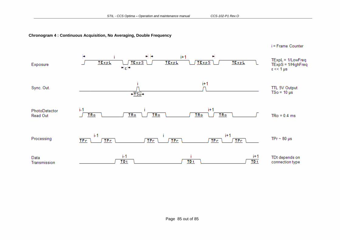
STIL - CCS Optima – Operation and maintenance manual CCS-102-P1 Rev.O
Page 85 out of 85
Chronogram 4 : Continuous Acquisition, No Averaging, Double Frequency