cellular dynamics simulations of bacterial...

Chemical Engineering Science, Vol. 48. No. 4, pp. 687-699, 1993. ooos-2509/93 55.00 + 0.00 Printed in Great Britain. Q 1992 Pngamm Press Ltd

CELLULAR DYNAMICS SIMULATIONS OF BACTERIAL CHEMOTAXIS

PAUL D. FRYMIER, ROSEANNE M. FORD’ and PETER T. CUMMINGS Department of Chemical Engineering, Thornton Hall, University of Virginia, Charlottesville,

VA 22903442, U.S.A.

(First received 20 September 1991; accepted in revised form 2 June 1992)

Abstract-The temporal and spatial evolution of the density of populations of chemotactic bacteria have previously been modeled by phenomenological cell balance equations based on cell motion restricted to one dimension. These one-dimensional balance equations have been used to interpret the results of experiments involving three-dimensional motion of bacterial populations with symmetry in two of the three dimensions. We develop a computer simulation to rigorously model the movement of a large population of individual chemotactic bacteria in three dimensions. Results of the simulation are compared with results using a one-dimensional phenomenological model in order to verify the range of validity of this model under situations involving one-dimensional gradients of chemical attractants.

1. INTRODUCTION

The migration of bacterial populations plays an important role in many ecological processes such as nitrogen fixation, pathogenesis of infection, formation of biofilms and the degradation of chemical wastes in the environment (bioremediation) (Chet and Mitchell, 1976). However, the extent to which migration affects these natural processes is not well understood. One approach toward quantifying this behavior is through the development and application of accurate mathematical models. The transport properties contained within these models are needed for the design of effective processes which would exploit the migration and redistribution of bacterial populations in natural environments. For example, bacterial migration is important for facilitating contact between the bacteria and the contaminant to be degraded for in situ ap- plications of bioremediation.

River0 et al. (1989) have proposed a mathematical model (hereafter referred to as the RTBL model) describing the migration of bacteria in the presence of chemical gradients. Their model includes two transport coefficients: one to characterize random motion in the absence of chemical gradients and another representing the directed motion associated with the presence of a chemical gradient. An experimental apparatus was designed by Ford er al. (1991) to determine values for the transport properties which are utilized in the RTBL model. However, the model was derived for the case of motion in only one dimension, while bacteria within the experimental apparatus ac- tually move in three dimensions. Although the RTBL model was shown to agree well with experiments under conditions of steep one-dimensional chemical gradients, it has been subsequently shown (Ford and Cummings,1992) that the RTBL model cannot be reconciled with a more mathematically rigorous (but more difficult to apply in practice) three-dimensional

‘Author to whom correspondence should be addressed.

cell balance approach except in one limiting case-specifically, the limit of a small one-dimensional attractant gradient implying symmetry in the remaining two dimensions. It is our objective in this paper to study the effect of simplifying assumptions implicit in the RTBL model on solutions obtained under the conditions of steep chemical gradients real- ized in the experiments of Ford et al. This is accomp- lished through the application of a cellular-level simulation technique to problems where we expect the model to perform the least satisfactorily based on the series expansion analysis of Ford and Cummings (1992). Since the transport properties will be used for design of improved processes, it is critical that the models we use to interpret experimental data for de- termining these coefficients be accurate.

With these tools available, those processes which most strongly influence bacterial behavior in natural settings can be identified and appropriate strategies for design and control can be implemented.

In Section 2, we review some of the previous works in the area of bacterial chemotaxis. In Section 3, we describe the methodology of the computer simulation program. The simulation results are compared with RTBL in Section 4 for conditions similar to those in the experimental apparatus developed by Ford et al. (1991) to study the migration of bacterial populations. The comparisons are performed over a range of parameters characterizing the attractant concentration and bacterial sensitivity to the attractant in order to .delineate the regions where the RTBL model is valid. In Section 5 we state our conclusions.

2. BACKGROUND

Peritrichous bacteria such as Escherichia coli and Salmonella typhimurium are able to move in a fluid medium via the coordinated rotation of approxim- ately 6-8 flagella attached to the perimeter of the cell. The movement of these bacteria can be described as alternating between two distinct phases: “running”

687

688 PAUL D. FRYMIER et al.

and “tumbling” (Berg and Brown, 1972; Macnab and Koshland, 1972; Spudich and Koshland, 1975). Dur- ing the running phase, the cell’s flagellar bundle ro- tates counterclockwise in a coordinated fashion and the cell moves in a nearly straight path. The duration of a typical run is of the order of l-10 s. In the tumbling phase, the rotation of the flagella reverses and the bundle uncoils so that no coordinated linear motion occurs and the cell spins in place. The duration of the tumbling phase is of the order of 0.1 s. As a result of tumbling the cell reorients itself according to a turn angle distribution, which has a slight bias in the direction the cell was moving prior to tumbling (Berg and Brown, 1972; Macnab and Koshland, 1973), and then begins a new run. In a uniform environment, the swimming pattern resembles a three- dimensional random walk similar to Brownian motion in molecular diffusion. This motion is described by the term random motility.

In the presence of a concentration gradient of an attractant (food sources such as sugars or amino acids, for example), bacteria are able to bias their random walk by changing their tumbling frequency (Macnab and Koshland, 1972; Spudich and Koshland, 1975). When moving toward an area of increasing (decreasing) attractant concentration, cells decrease (increase) their tumbling frequency, thereby increasing (decreasing) the lengths of their runs in the direction of increasing (decreasing) attractant concentration. In this way, a population of cells moving within an attractant gradient will exhibit a net movement toward the attractant source. This overall directed motion is called chemotaxis. The ability of chemotactic bacteria to direct their motion enables them to move to more favorable environments by swimming toward increasing concentrations of nutri- ents, giving these bacteria a competitive advantage over nonmotile bacteria (Kelly et al., 1988).

A complete mathematical description of the motion of a population of chemotactic bacteria requires a set of cell balance equations along with constitutive relationships which relate the quantities in the cell balance equation to the properties of the cells and their motion. The three-dimensional cell balance equations of Alt (1980) are the most general. Letting a@, & 7, t) be the number density of cells per unit volume at position r moving in direction s with run time t at time t, Alt’s fundamental equation is

au@, fi, 7, t) Wr, .% 7, 0

at =- ds

- 8. VJu(r,t)a(r, L 2, 01 - B(r, 8, z, Mr, 6, z, 4 (1)

for 7 > 0 and

a(r, 8, 0, t) = ss

m P(r, $ ,T, tMr, 8’7 7, t) 0

x k(r, $‘, t; .Q) dB’ ds (2)

for z = 0. Here, B( r, 0, 7, t) is the probability per unit time that a cell moving in direction d at r at time t with run time z (counted from the beginning of the run)

tumbles at r at time t. The probability that a cell chooses the direction gz as its new direction after tumbling is k(r, &, t; ~3,). The subscript r emphasizes that the divergence operator V, is with respect to the spatial coordinate r. The swimming speed of the bacteria is o and is known from experimental observations to be relatively constant over a range of attractant concentrations (Nossal and Chen, 1973; Berg and Brown, 1972). Equation (1) states that the rate of change in the population of cells at r at time t moving in direction B with run time 7 is given by a term which reflects the loss of cells in the population due to changes in the run time, a term that reflects the change in the population due to convection, and a term that reflects the loss to the population due to cells tumbling with probability j?. Equation (2) states that one obtains an initial (z = 0) population of cells moving in direction d by considering cell populations which were moving in another direction 61’ with run time z which tumbled at time t, represented by the product B(r. 13’, t, t)a(r, $‘, 7, t), and multiplying by the probability that the cell moves in the direction L after tumbling, given by k(r, I’, t; a). This product is integ- rated over all directions I’ and all run times 7.

Segel(1977) and River0 et al. (1989) have developed simpler phenomenological models based on individual cell motion in one direction only. The one- dimensional balance equations of Segel are

an+ -= at

- 6 (sn+) + p-n- - p+n+

&- a ~ = &Sn-) + p+n+ -p-n- at

where n+(z, t) is the density of cells at point z at time t moving in the positive z direction and n- (z, t) is the density of cells at point z at time r moving in the negative z direction, s is the one-dimensional, scalar swimming speed of the bacteria, p+ = p+(z, t) is the probability per unit time that a cell moving in the positive z direction tumbles and becomes a cell moving in the negative z direction and p- = p-(z, t) is the probability per unit time that a cell moving in the negative z direction tumbles and becomes a cell moving in the positive z direction.

The RTBL model is based on the cell balance equations of Segel. Under the assumption that the phenomenon of tumbling is a Poisson process (Berg, 1983), the tumbling probability p, is equal to the inverse of the mean run time,

1

P’=<r)L (5)

This assumption is supported by the experimental work of Berg and Brown (1972). River0 et al. write this equation in one dimension as

*_ 1 Pt --

<z*> (6)

where p: = p#* (z, t) is the probability that a cell moving in the + z direction tumbles and <r* > is the mean

Simulations of bacterial chemotaxis 689

run time for cells moving in the + .z directions, re-

spectively. In addition, River0 et al. propose

P * = P?Pr (7)

where pr is the probability that a cell reverses direc-

tion after tumbling. The mean run times (z’ } are then related to the attractant concentration a and its gradient by

where <rz > is the mean run time of cells moving in the & direction, K, is the dissociation constant for the attractant-receptor binding and #’ is the one-dimensional chemotactic sensitivity parameter. In the RTBL model, eqs (6)-(g) form a set of constitutive equations for Segel’s cell balance equations.

As shown in Appendix A, eq. (8) is a mathematical simplification of the expression for bacterial motion in three dimensions given by

In cc> _ id” & (70) r (Kd + a)2

6*Va (9)

where <to> is the mean run time in the absence of an attractant gradient and xaD is the three-dimensional analogue of ~4~. For a discussion of the derivation of eq. (9) above we refer reader to Appendix A. Substi- tuting eq. (5) into eq. (9) and rearranging, we have

3D Kd p, = pt, exp - xO u (K#j + ay

L-Vu >

(10)

where

1 pt0 =-,

<To> (11)

In the one-dimensional RTBL model,

(12)

where

(13)

so the complete RTBL model is the set of equations (3), (4), (6), (7) (12) and (13). For a discussion of the approximate nature of eq. (12), we refer the reader to Appendix A. The RTBL mode1 was applied to the interpretation of experimental data by Ford et al. (1991) for E. coli K 12 responding to fucose. The experiments were carried out in a stopped flow diffusion chamber (SFDC) shown schematically in Fig. 1. For assays of chemotactic bacteria in the SFDC, a suspen- sion of bacteria at concentration b. is pumped at a uniform rate into the upper port of the chamber and a mixture of attractant at concentration a, and bacteria at concentration b. is pumped at a uniform rate into the lower port. Muid exits through ports at the centerline of the chamber and the flow rates are con- trolled by a dual piston syringe pump so that, for times t < 0, the two impinging streams form a step

-9-

stopped-flow diffusion chamber

Fig. 1. Schematic representation (left) of the SFDC used by Ford and co-workers. Impinging flow from the upper and lower ports creates an initial step change in attractant gradient at the center of the chamber and a uniform distribution of bacteria. The approximate dimensions of the chamber are 4 x 2 x 0.2 cm. On the right is an exploded view of the simu-

lation box which is referred to later in the text.

change in the attractant concentration at the center of the chamber. At time t = 0, flow into and out of the SFDC is stopped and the attractant begins to diffuse into the upper-half of the chamber generating a time- dependent gradient. As bacteria sense the gradient, a band of high cell density forms where the gradient is large and moves downward in the chamber to regions of higher attractant concentration. The experimental geometry is one of symmetry in two dimensions (the x and y directions in Fig. 1) with an attractant gradient in the third dimension (the z direction).

Ford and Cummings (1992) studied in detail the relationship between the three-dimensional balance equations of Alt, eqs (1) and (2), and the one-dimensional equations of Segel, eqs (3) and (4), the latter being the basis for the RTBL model. Ford and Cummings showed that the Segel equations could only be derived rigorously from Alt’s equations when the motion of the bacteria is confined to one dimension. They considered three-dimensional systems with an attractant gradient in the z-coordinate direction and symmetry in the other two (x, y) coordinate directions so that

V,U = (0,0, aa/&). (14)

For cases of symmetry (as opposed to confinement to one dimension), Ford and Cummings showed that the Alt equations could not be reduced to the Segel equations except in the limit of small a, where,& is defined by

pt = psev(- 4. (15)

By comparing eq. (15) with eq. (10) and making use of eq. (14), E can be written as

&if Kd Ecos* D (Kd + a)2 az (16)

where 8 is the angle made by the direction vector $ with the z-axis. By perturbatively expanding in E, a reduced form of the Alt equations (obtained by


integrating over T, x and y), Ford and Cummings obtained

-/31n$k+- + /3in;k-+

(17)

-PPin;k_+ + /3in$k+_

(18)

where /I1 is the tumbling probability, k + _ is the probability that a cell moving in the positive z direction becomes a cell moving in the negative z direction after tumbling and k_ + is the probability that a cell moving in the negative z direction becomes a cell moving in the positive z direction. The subscript 0 indicates that these are the leading order terms from series expansions in the parameter E.

Ford and Cummings’ analysis clarifies the relationship between the one-dimensional cell speed s in the Segel equations and the three-dimensional ccl1 speed u that is determined experimentally. From their analysis, it is apparent that the correct speed to use in the one-dimensional equations is the observable three-dimensional cell speed u divided by 2 rather

than fi recommended by Segel (1979) and used in the analysis of Ford et al. (1991) and Ford and Lauffenburger (1991). Ford and Cummings noted that although this correction to the cell speed is small, it would affect the value of the population parameters inferred from experiments. Using eqs (A9) and (A6) from Appendix A and the relationship

0 = 2s

derived by Ford and Cummings, we have

(19)

x;n = VV2Nr = 4x;n (20)

where v is a proportionality constant describing the fractional change in mean run time per unit time rate of change in cell surface receptors that are bound to attractant molecules. We note that using the relationship s = v/d = 0.577~ instead of the correct relationship s = 0.5~ results in s being overestimated by 15.5%. It would, consequently, result in the xl” inferred from experiment being underestimated by 25% according to the relationship in eq. (20).

The studies of Ford et al. (1991) and Ford and Lauffenburger (1991) involved comparison of the experimentally measured bacterial density with the predictions of the RTBL model. For appropriately chosen values of #‘, there is good agreement between RTBL and experiment. Several approximations and/or assumptions are implicit in using the RTBL model: first, use of the approximate one-dimensional balance equations, eqs (3) and (4); second, the diffusion approximation (River0 et al., 1989) which enables the RTBL model equations to be solved numer- ically at the macroscopic level; third, the model for the tumbling probability, eq. (lo), which involves a proposed mechanism for the way in which bacteria sense and respond to their environment; and, fourth, the

simplification of the tumbling probability to the one- dimensional form, eq. (12), as described at the end of Appendix A. Of these four, three are mathematical approximations (first, second, and fourth) and one is a phenomenological assumption. One role for the cellular dynamics simulations is to test the validity of the mathematical approximations and is the focus of this paper. The validity of the phenomenological assumptions can be tested by comparing the simulation results with experiments; however, this is not the sub- ject of this paper.

Since the RTBL model does agree well with experiment, a question then naturally arises. Is the agreement of RTBL with experiment fortuitously caused by cancellation of two or more sources of error intro- duced by the phenomenological assumption for the tumbling probability and the mathematical approximations? The most straightforward way to answer this question is to perform a cellular-level simulation of bacterial motion corresponding to the experimental situation (bacteria moving in three-dimensional space in the presence of a one-dimensional attractant gradient) that eliminates the mathematical approximations by using the general (three-dimensional) tumbling probability model, eq. (10). The degree to which the RTBL model predictions and the simulation agree is then a measure of the validity of the mathematical approximations and, thus, the validity of the RTBL model in describing real three-dimensional systems with attractant gradients in one spatial direction.

Computer simulations of the motion of individual bacteria have been reported by several researchers. Berg (1983, 1988) performed simulations to illustrate the random walks generated by single cells assuming Poisson statistics for the tumbling probability and a simple approximation to the bias in the turn angle distribution. Bornbusch (1984) and Bornbusch and Conner (1986) investigated the effect of limiting the turning field size of a cell on its ability to locate an attractant source. Tankersley and Conner (1990) performed simulations of single-cell migration to illustrate how the differences between various cell types in the mechanisms used to move toward an attractant source resulted in markedly different patterns of migration. In the present work, we develop a computer simulation methodology which rigorously describes the three-dimensional motion of individual chemotactic bacteria for the situation present in the SFDC experiments. Unlike the previous computer simulations just described, we simulate a large population of bacteria (20,000 cells) and incorporate the experimentally measured turn angle distribution into the mechanism for reorienting the cells after tumbling. The results of the simulation are compared with those obtained using the RTBL model which involves the assumptions and approximations detailed above.

3. SIMULATION METHODOLOGY

After setting the appropriate initial conditions, bacterial movement is simulated by performing three calculations for each individual bacterium at each

Simulatiorwof bacterial chemotaxis 691

time step. First, it is determined whether or not the cell tumbles. Second, if the cell tumbles then its new direction is chosen; if it does not tumble, its direction is maintained. Third, the cell’s new position is com- puted based on its direction vector, swimming speed and the time step. The implementation of these three steps and other details of the simulation are described in this section.

The simulation “box” is given an initial uniform random distribution of bacteria. Letting b(r, r) he the bacterial density at position rat time t, then the initial concentration b(r, t = 0) (see Fig 1) is given by

b(r, t = 0) = 60, - h/2 d x d h/2

- w/2 < y & w/2

- lf2 < 2 < l/2. (21)

An initial bacterial concentration of b, = 2 x 10’ cells/cm3 was used in the experiments of Ford et al. (1991); however, for the simulation results presented here, we used an initial concentration of bacteria of b. = 2 x lo6 cells/cm” in order to reduce the calculations necessary at each time step by an order of magnitude. The bacteria are assigned initial direction vectors at random. A step change along the z-axis at time t = 0 in the concentration of an attractant, a, exists such that

a(z, r = 0) = 0, - l/2 $ 2 < 0

a(z, t = 0) = ao, 0 c z Q l/2 (22)

a(z,t)=T[l +erf(&)]

t>o, -1/2<z<l/2. (23)

where a, is the initial attractant concentration intro- duced into one-half of the chamber, D is the diffusion coefficient of the attractant, z is the position along the z-axis and t is time. The solution given above for t > 0 can be found in Crank (1979). For t > 0, the motion of each bacterium is modeled as an independent, three- dimensional, biased random walk.

That the motion of each bacterium can be considered independent of the motion of other bacteria is justified by noting that the ccl1 densities used in the SFDC experiments are low enough that intercellular distances are at least an order of magnitude greater than cellular diameters. However, at much higher cell densities (by an order of magnitude or more), hydrodynamic interactions among swimming bacteria may be significant (Guell et al., 1988). In such cases, the application of this simulation technique would require additional terms in the equations of motion to account for hydrodynamic interactions between the bacteria. The position ri of the bacterium i at time t + At, where At is the time step in the simulation, is given by

r,(t + At) = s(t) + &,At (24)

where u is the three-dimensional swimming speed of the bacterium and Bi is the unit vector in the direction of motion of the bacterium. The simulation box

employs periodic boundary conditions (Allen and Tildesly, 1987). If the cell moves out of the box, it is repositioned so that it reenters at the opposite wall, retaining a constant number of cells in the simulation box. The length of the simulation box in the direction of the attractant gradient (the z direction) is 0.8 cm. This is sufficiently large to ensure that the attractant concentration is uniform at the ends of the box (z = f 0.4 cm), at which points the cell density re- turns to the bulk density b. .

The unit direction vectors for the bacteria evolve in time according to

where

$(r + At) = ~i$(t) + (1 - ni)bl (25)

;li = @[pi(t + At) - ptAtJ. (26)

In this equation, pi is a random number chosen at time t + At from a uniform distribution on [0, 11, p, is the tumbling probability, .$ is chosen randomly from the distribution for the change in direction after tumbling obtained by experimental observations of single cells by Berg and Brown (1972), and 0 is the Heaviside function, defined as

O(x) = 1 0, x-co 1, x2-0.

Details on the method of choosing di are provided in Appendix B. Equation (26) implies that

li = 1 if pi 2 prAt (28)

li = 0 if p1 < ptAt (29)

so that a bacterium has probability ptAt of tumbling and probability (1 - pt At) of continuing its run. Thus, the tumbling probability in a zero gradient is constant and consistent with a Poisson distribution. The time step used in the simulation is At = 0.1 s, the time corresponding to Q, the experimentally observed duration of a tumble. Therefore, the tumbling process is effectively instantaneous in our simulation.

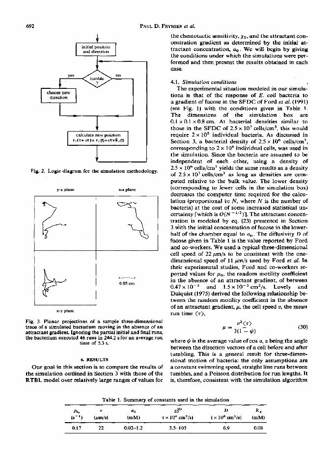
The logic diagram in Fig 2 summarizes the methodology described in this section. The simulation box is first initialized. At the start of the simulation loop, each bacterium decides whether or not to tumble [according to eq. (26)]. Based on whether or not it tumbles, either a new direction is chosen or the bacterium continues its run in the same direction. Finally, the bacterium moves to a new position based on its swimming speed and direction vector using an Euler’s integration of the equation of motion. Figure 3 shows the path of a single cell generated by applying the simulation algorithm in the absence of a chemical gradient over a period of 25OOAt, where At = 0.1 s. The cell swimming speed (22 pm/s) and zero-gradient tumbling probability (0.17 l/s) are the same as for the simulations reported in Section 4. Note that periodic boundary conditions were not implemented in this sample trace.

In the next section, we discuss the results of the simulation.

692 PAUL D. FRYM~ER et al.

choose new direction

I I

Fig. 2. Logic diagram for the simulation methodology.

initial position and direction

I4

y-z plane x-z plane

- 0.05 cm

x-y plane

Fig. 3. Planar projections of a sample three-dimensional trace of a simulated bacterium moving in the absence of an attractant gradient. Ignoring the partial initial and final runs, the bacterium executed 46 runs in 244.2 s for an average run

time of 5.3 s.

4. RESULTS

Our goal in this section is to compare the results of the simulation outlined in Section 3 with those of the RTBL model over relatively large ranges of values for

the chemotactic sensitivity, x0, and the attractant concentration gradient as determined by the initial attractant concentration, a,,. We will begin by giving the conditions under which the simulations were performed and then present the results obtained in each case.

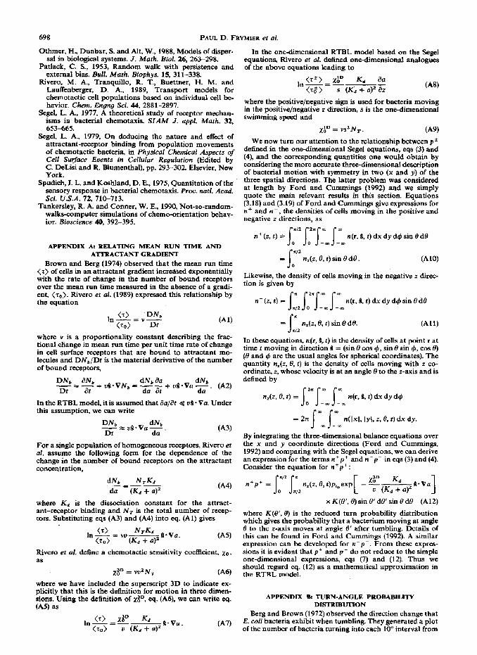
4.1. Simulation conditions The experimental situation modeled in our simula-

tions is that of the response of E. coli bacteria to a gradient of fucose in the SFDC of Ford et al. (1991) (see Fig. 1) with the conditions given in Table 1. The dimensions of the simulation box are 0.1 x 0.1 x 0.8 cm. At bacterial densities similar to those in the SFDC of 2.5 x 10’ cells/cm’, this would require 2 x 10’ individual bacteria. As discussed in Section 3, a bacterial density of 2.5 x lo6 cells/cm3, corresponding to 2 x lo4 individual cells, was used in the simulation. Since the bacteria are assumed to be independent of each other, using a density of 2.5 x lo6 cells/cm3 yields the same results as a density of 2.5 x 10’ cells/cm’ as long as densities are com- puted relative to the bulk value. The lower density (corresponding to fewer cells in the simulation box) decreases the computer time required for the calcu- lation (proportional to N, where N is the number of bacteria) at the cost of some increased statistical un- certainty [which is O(N -“‘)]. The attractant concentration is modeled by eq. (23) presented in Section 3 &th the initial concentration of fucose in the iower- half of the chamber equal to ao. The diffusivity D of fucose given in Table 1 is the value reported by Ford and co-workers. We used a typical three-dimensional cell speed of 22 ,um/s to be consistent with the one- dimensional speed of 11 m/s used by Ford et al. In their experimental studies, Ford and co-workers reported values for p,,. the random motility coefficient in the absence of an attractant gradient, of between 0.47 x 10e5 and 1.5 x 10e5 cm2/s. Lovely and Dalquist (1975) derived the following relationship between the random motility coefficient in the absence of an attractant gradient, p, the cell speed v, the mean run time (z},

02<r> P = 3(1 - +)

(30)

where I(/ is the average value of cos c(, c( being the angle between the direction vectors of a cell before and after tumbling. This is a general result for three-dimensional motion of bacteria: the only assumptions are a constant swimming speed, straight line runs between tumbles, and a Poisson distribution for run lengths. It is, therefore, consistent with the simulation algorithm

PI. (s-‘)

0.17

Table I. Summary of constants used in the simulation

”

(I$

XT D

(ccmls) ( x 104 cm2/s) {x 106 cm’/s)

22 0.02-l .2 3.5-105 6.9

Kd

(mM)

0.08


and with Alt’s general three-dimensional cell balance equations, eqs (1) and (2), under the additional assumption of a constant-cell swimming speed. We used a seventh-order polynomial fit (see Appendix B for further details) to the experimental data of Berg and Brown (1972), and determined that 9 = 0.36. Using this value of + and values of 1.5 x 10e5 cm’/s for p0 and 22 pm/s for V, yields a value for <t> of 6.0 s by eq. (30). For a Poisson process, this corresponds to a tumbling probability of pI, = 0.17 l/s in the absence of a gradient, which is the value that used in our simulations. A time step of At = 0.1 s was used. For this time step, a bacterium in the simulation moving in a isotropic medium will, on an average, tumble every 58 time steps. The values of the parameters used in the simulation are summarized in Table 1.

One test of our simulation methodology is to calcu- late the random motility c from the simulation and check that it matches the value given by eq. (30). We performed a simulation in the absence of an attractant gradient and calculated the mean squared displacement Q(t) of the bacteria defined by

f-l(t) = L N ,il CrAt) - ri(W2 _ (31)

According to the Einstein relation (Allen and Tildesly, 1987),

Q(t) --+ 6pt (32)

so that at long times R should become linear in t with slope 6~. As can be seen in Fig. 4, n(t) is indeed linear in t at large t. The slope implies a value of 1.55 x 10-5cm2/s for p which is within 3% of the correct value. This suggests that the simulation me,thodology is very accurate. Note that at short times, R is quadratic in t. By fitting Q(r) to ut2 for t -z 2 s, we find a = 452 pm2/s2 which is within 7% of u2, consistent with the short-time analysis of the RTBL model as presented by Othmer et aZ. (1988). The crossover from n(t) - t2 to n(t) - t corresponds to the transition to the diffusion regime in which the diffusion approximation, discussed by River0 et al. (1989), is valid. Hence, the fact that n(t) becomes linear in t for t r 10 s suggests that the diffusion approximation is satisfied at relatively short times. The diffusion approximation is utilized in the macroscopic version of the RTBL model solved by Ford et

7

6 2cm cells

5

R (0

(n IO’ cmy

4 I 3

2

1

00 20 4 60 80

time (set)

a$$t&, 0.2 jz%k] [-z] concentration

IO” 1ti3 1O-2

chemotactic sensitivity (cm’/sec)

Fig. 4. Mean-squared displacement fi as a function of t. Fig. 5. Summary plot of cases presented.

al. (1991) and the simulation results suggest that the diffusion approximation should be accurate.

The macroscopic form of the RTBL model which follows from the diffusion approximation (River0 et al., 1989) was implemented in a finite difference program using a predictor-corrector method (Ford, 1989). As discussed in Section 2, the RTBL model is expected to show the most deviation from the simulation for large attractant gradients and large values of the chemotactic sensitivity coefficient, since the three- dimensional equations simplify to an analogue of the one-dimensional phenomenological model only in the limit of small E, eq. (16). The range of values of the parameters x,, and Q,, over which we performed simulations and comparisons with the RTBL model in- clude the lower (0.01 mM) and upper (1 .O mM) ranges of a0 studied experimentally with the SFDC and the lower (3.5 x 10m4 cm*/s) and upper (105 x 10m4 cm2/s) limits on xiD measured experimentally (Ford, 1992; Mercer, 1991). The cases that are considered in this study are summarized in Fig. 5. We did not consider higher values of aO, since for attractant concentrations significantly above 10 times the dissociation constant for the attractant-receptor binding, I&, the receptors available for sensing concentration gradients become saturated (Koshiand, 1980) and the cell no longer responds chemotactically. Simulations were also performed for intermediate values of the parameters n, and x0 to determine if significant differences could be observed between the simulation and the RTBL model. The results yielded similar trends to those presented here.

In view of the Ford and Cummings (1992) analysis, it is interesting to consider the relative values of E [see eq. (16)] implied by the four cases considered. We can write E in the form

E=EOcoSe~

where Ed, which is dimensionless and angle-independent, is given by

E _ E &a0 O - ul (Kd + a)”

(33)


Clearly, because of the gradient term a(a/u,)/a(z/~), which varies from f co at z = 0 and t = 0 to essen- tially zero at z = + 112, the value of E can be very large and will depend on position and time. As the attractant profile relaxes with time, e will become small at all positions. Thus, for given values of xaD and a0 there will be a t-dependent range of z which contracts as t increases and inside of which G will be large. Based on the Ford and Cummings (1992) analysis, this might be the region for which the RTBL model may not be successful since the Alt equations simplify to the Segel equations only under the assumption of small E. The larger Q, is, the greater will be the range of z and t included in this region. By evaluating e0 at z = 0, where a = a0/2 for all t, we can obtain a dimensionless measure of the expected ap- plicability of the RTBL model, larger values of e0 implying a smaller region of z and t over which RTBL might be applicable. For the four cases shown in Fig. 5, cases 14 yield values for s0 of 0.09X,2.9,0.041 and 0.039, respectively. On this basis, we might expect that RTBL would be least applicable to case 2 and most applicable in cases 3 and 4. We should also note that E,, has its maximum value as a function of a,, at

a0 = 2K d = 0.16 which is near the value of 0.2 for cases 1 and 2. In Fig. 6 we show the quantity cl = @OS 0 as a function of z and t for case 1. As is evident from this figure, e1 is significantly larger than zero over significant ranges of z and t. Thus, a priori one would expect that the RTBL model would not be very accurate.

First, we consider values of a, and x0 that are similar to those used in the SFDC experimepts of Ford et al. (1991). In Fig. 7 the RTBL model with s = v/2 and xAD = xsD/4 is compared with

the simulation results for a0 = 0.2 mM and x$” = 3.5 x 1O-4 cm’/s. These relationships, derived by Ford and Cummings (1992), are the proper ones between the three-dimensional and one-dimensional parameters as discussed previously in Section, 2. They are used in the results for all cases presented in this work. The points at which cell densities from the simulation are plotted in the figure are the average of the density in a “sampling bin” 0.01 cm wide centered around the point. Sampling is implemented over 50 time steps (which corresponds to 5 s), so the density reported for a point at a given time is the average density in the sampling bin over the sampling period. The statistical error associated with the simulation causes the curve representing the simulation results to be a little noisy. The RTBL model agrees closely with the simulation in this case. The peak in the cell density profile is the result of a high-density band of cells that forms where the concentration gradient is high. The trough in the density profile is the result of cell de- pletion in the region behind the advancing concentration gradient as cells move with the gradient. These phenomena are also observed in experimental studies (Ford et al., 1991).

For the second case, shown in Fig. 8, we used a value of ~3” = 105 x 10m4 cm2/s, which is 30 times larger than the first case and the same initial attractant concentration a, as the previous case. Note that the scale on the vertical axis has been changed to allow for the higher peak value of the bacterial density at this value of x0. Again, the simulation results agree well with those of the RTBL model.

Next we look at the efiect of the initial concentration, uo. on the simulation and the RTBL model results. In Fig. 9, x0 1s 3D . held fixed at 3.5 x 10V4 cmf/s

0.4 I I I I I I I

0.2 -

fl c 0.5

-0.4 1 I I I I I I I 0 * 100 200 300 400 500 600 700

t (sets)

Fig. 6. Regions in the z-t plane inside which the quantity .s, has ranges 61 ‘z 1, .sl > 0.5 and .s, < 0.5.


2 2

b/b0 1.5 1.5

1 1

0.5 0.5

2.5 t time= 6.0 min I 2.5 t time= 12.0 min

2 2

b/b0 1.5

1

0.5

position (cm) position (cm)

Fig. 7. Comparison of RTBL and simulation results for a0 = 0.2mM and xiD = 3.5 x 10T4 cm’/s at t = 0.5, 3, 6, 12 min. The smoother of the curves represents the results from RTBL.

b/b0

5

4

3

2

1

0 -0.4 -0.2 0 0.2 0.4

4

3

2

1

0 -0.4 -0.2 0 0.2 0.4


Fig. 8. Comparison of RTBL and simulation results for a,, = 0.2 mM and xiD = 105 x 10m4 cm2/s at t = 0.5 and 6 min. Note the change of scale on the vertical axis.

2.5 t

time= 0.5 min time= 6.0 min

b/w lJ-

I Ohk+Yik- 0.4 -0.4 . 4


Fig. 9. Comparison of RTBL and simulation results for cl0 = 1.2 mM and #’ = 3.5 x 10e4 cm% at t = 0.5 and 6 min.


2


Fig. 10. Comparison of RTBL and simulation results for no = 0.02 mM and xi” = 3.5 x 10m4 cm’/s at t = 0.5 and 6 min. Note the change of scale on the vertical axis.

as in the initial case and a0 is increased to 1.2 mM, 6 times the value used in the first case. As in the two previous cases, the agreement between the two solutions is very good.

In case 4, we look at the effect of lowering the value of aO. Figure 10 shows the results obtained using a0 = 0.02 mM, while holding ,#’ fixed. The simulation results shqw a larger maximum value of the bacteria density than does the RTBL model, but tak- ing into account statistical inaccuracies the deviation of the RTBL model from the simulation is quite small.

Our earlier discussion of the expected accuracy of the RTBL model suggested that the RTBL model would agree least with the simulatiou for case 2, agree most for cases 3 and 4, but for all cases show some deviation for a range of z and t depending on the values of u. and x :” However, it is apparent that the , RTBL model agrees very well with the simulation for ail the cases and for most values of z and t. This suggests that the validity of the Segel equations cannot be judged solely on the basis of the magnitude of the perturbation parameter E.

5. CONCLUSION

In Section 4, we considered the effect of the parameters a, and x0 on the simulation and the RTBL model to determine the range of validity of one-dimensional phenomenological models for conditions involving symmetry in two dimensions. We varied the range of x$ from 3.5 x lo-“ to 105 x 10e4 cm’/s. The initial concentration a0 was varied from 0.02 to 1.2 mM. In all cases presented here, the agreement between the three-dimensional simulation and the one-dimensional RTBL model is very good. There are three possible explanations for this good agreement: the first is that the ranges of z and t over which E is large are, in practice, small compared to the full ranges of z and t; the second is that, in the regions where E is large, the motion of the bacteria becomes effectively one-dimensional, so that a one-dimensional model is appropriate; the third is that the coefficients of the higher-order terms in the per-

turbative expansion are small, so that the higher-order terms are negligible even when E is large. It is probable that some combination of these mechanisms is involved. In any event, our comparisons show that the assumption of small c necessary to reduce the more rigorous, three-dimensional equations of Alt to the one-dimensional phenomenological RTBL model does not inhibit its u$e in accurately modeling situations involving two dimensions of symmetry.

It should be emphasized, however, that the very good agreement between the one-dimensional model and the three-dimensional simulation only follows when one uses the relationships between the three- dimensional chemotactic sensitivity and cell swimming speed and their one-dimensional analogues that follow from the Ford and Cummings (1992) analysis. These relationships should be used in all future works when parameters for one-dimensional phenomenological models are obtained by experimental measurement.

Acknowledgements-This research was performed by RMF under the sponsorship of the U.S. Department of Energy, Environmental Restoration and Waste Management Young Faculty Award Program administered by Oak Ridge Asso- ciated Universities. This research was performed by PDF under appointment to the Environmental Restoration and Waste Management Fellowship Program administered by Oak Ridge Associated Universities for the U.S. Department of Energy. We thank the anonymous reviewers for very helpful and detailed suggestions on an earlier version of this uaDer.

C

D h k k+-

NOTATION

attractant concentration, mM bacterial density in experiment and simulation, cells/cm3 coefficient in the polynomial approximating the probability distribution of cos c( diffusion coefficient for attractant, cm*/s simulation box height in x direction, cm probability of turning to a specified direction probability that a bacteria moving in the positive z direction will change to the negative z direction after tumbling


probability that a bacteria moving in the REFERENCES negative z direction will change to the positive z direction after tumbling Allen, M. P. and Tildesly, D. I., 1987, Computer Simulations dissociation constant for attractant-receptor ofliquids. Oxford University Press, New York.

binding, mM Alt, W., 1980, Biased random walk models for chemotaxis

simulation box length in z direction, cm and related diffusion approximations. .I. Math. Biol. 9, 147-177.

coordinate transformation matrix Berg, H. C., 1983, Random Walks in Biology. Princeton one-dimensional bacterial density in Segel’s University Press, Princeton, NJ.

equations, cells/cm’ Berg, H. C., 1988, A physicist looks at bacterial chemotaxis.

number of receptors bound to attractant Cold Springs Harbor Symposia on Quantitatiue Biology

molecules 53, 1-9.

Berg, H. C. and Brown, D. A., 1972, Chemotaxis in number of cell surface receptors Escherichia coli analvsed bv three-dimensional trackinn.

k-+

Kd

1 M n

NT P*

Pr

Pt r

: t v W

x, Y, z

probability that a cell moving in the 4 z Nature 23!3,50&504: - direction tumbles and becomes a cell moving Bombusch, A. H., 1984, Turning field size and its effects

in the i z direction, l/s upon computer simulated klinotactic orientation. J.

probability that a bacterium reverses after Theoret. Biol. 107, 151-163.

Bombusch, A. H. and Conner, W. E., 1986, Effects of self- tumbling reduced probability of tumbling, l/s position vector, cm one-dimensional cell speed, cm/s

steered turn size and turn bias uvon simulated chemo- klinotactic behavior. J. Theoret. Biol. 122, 7-18.

Brown, D. A. and Berg, H. C., 1974, Temporal stimulation of chemotaxis in E. coli. Proc. natl Acad. Sci. U.S.A. 71, 1388-1392.

unit direction vector time. s

Chet, I. and Mitchell, R., 1976, Ecological aspects of microbial chemotactic behavior. Microbial. 30, 221-239.

------I -

three-dimensional cell speed, cm/s simulation box width in y direction, cm coordinate directions

Crank, J., 1979, The Mathematics 01 Di@ion, 2nd Edition. Clarendon Press, Oxford.

Yh.LA theses, Umversity 01 Pennsylvama.

Ford, R. M., 1989, Quantitative studies of bacterial motility

Ford, R. M., 1992, Mathematical modeling and quantitative

and chemotaxis using a stopped-flow diffusion chamber assay and an individual cell-based mathematical model.

characterization of bacterial motility and chemotaxis, in

-_- . __. “_ .

Metabolic and Physiologic Activities 01 Microorganisms (Edited by C. J. Hurst), pp. 177-215. Wilev, New York.

Greek letters

probability of tumbling, l/s angle of rotation of a bacterium’s direction

angle between a bacterium’s direction vector

vector before tumbling about its direction vector after tumbling

before tumbling and its direction vector after

a parameter used in the series expansions of Ford and Cummings (1992)

tumbling

angles of direction of a bacterium Heaviside function integer, either 0 or 1 random motility coefficient, cm’/s proportionality constant describing the fractional change in mean run time per unit time rate of change in cell surface receptors, s random number

__ Ford, R. M.-and Cummings, P. T., 1992, On the relationship

between cell balance equations for chemotactic cell populations. SIAM J. appl. Math. {in press).

Ford, R. M. and Lauffenburner, D.A.. 1991, Measurement of bacterial random motilityand chemotaxis coefficients. II. Application of single cell-based mathematical model. Biotechnol. Bioengng 37, 661672.

Ford, R. M., Quinn, J. A., Phillips, B. R. and Lauffenburger, D. A., 1991, Measurement of bacterial random motility and chemotaxis coefficients. I. Stopped-flow diffusion chamber assay. Biotechnol. Bioengng 37, 647-660.

Gueli, D. C., Brenner, H., Frankel, R. B. and Hartman, H., 1988, Hydrodynamic forces and band formation in swimming magnetotactic bacteria. J. Theoret. Biof. 135, 525-542.

Hammersley, I. M. and Handscomb, D. C., 1964, Monte Carlo Methods. Wiley, New York.

three-dimensional bacterial probability density, cells/cm3 bacteria run time, s tumbling time, s chemotactic sensitivity, cm’/s average value of cos (LX) the mean squared displacement for bacteria at time t divergence operator with respect to r

Kelly, F. X., Daosis. K. and Lauffenburaer. D.. 1988. Effect of bacteriai’ chemoiaxis on dynamics Gf microbial ‘eompeti- tion. Microbial Ecol. 16, 115-131.

Koshland, D. E., 1980, Bacterial Chemotaxis as a Model Behavioral System Raven Press, New York.

Lovely, P. S. and Dalquist. F. W., 1975, Statistical measures of bacterial motility and chemotaxis. J. Theoret. Biol. 50, 477496.

Macnab, R. M. and Koshland, D. E., 1972, The gradient- sensing mechanism in bacterial chemotaxis. Proc. nut1 Acnd. Sci. U.S.A. 69, 2509-2512.

Macnab, R. M. and Koshland, D. E., 1973, Persistence as

Superscripts and subscripts a concept in the motility of chemotactic bacteria. J.

1D one-dimensional Mechanochem. Cell Motility 2. 141-148.

Mercer, J. R., 1991, Quantitative characterization of the 3D three-dimensional effect of growth rate limitation on the chemotactic

+ the positive z-coordinate direction response of E. coli K12 to fucose. Master’s thesis, Uni-

- the negative z-coordinate direction versity of Virginia (unpublished).

0 in the absence of an attractant or an initial Nossal, R. and Chen, S. H., 1973, Effects of chemoattractants

on the motility of Escherichia coli. Nature New Biol. 244, value 253-254.


Othmer, H., Dunbar, S. and Alt. W., 1988. Models of disper- sal in biological systems. J. Math. Biol. 26, 263-298.

Patlack, C. S., I953, Random walk with persistence and external bias. Bull. Math. Biophys. 15, 311-338.

Rivero, M. A., Tranquillo, R. T., Buettner, H. M. and LautTenberger, D. A., 1989, Transport models for chemotactic cell populations based on individual cell be- hwior. Chem. Engng Sci. 44, 2881-2891.

Segel, L. A., 1977, A theoretical study of receptor mechanisms in bacterial chemotaxis. SIAM J. appi. Math. 32, 653-665.

Segel, L. A., 1979. On deducing the nature and effect of attractant-receptor binding from population movements of chemotactic bacteria, in Physical Chemical Aspects of Cell Surface Events in Cellular Regulation (Edited by C. DeLisi and R. Blumenthal), pp. 293302. Elsevier, New York.

Spudich, J. L. and Koshland, D. E., 1975, Quantitation of the sensory response in bacterial chemotaxis. Proc. natl. Acnd. Sci. U.S.A. 72, 71&‘713.

Tankersley, R. A. and Conner, W. E., 1990, Not-so-random- walks-computer simulations of chemo-orientation behavior. Bioscience 40, 392-395.

APPENDIX A: RELATING MEAN RUN TIME AND ATTRACTANT GRADIENT

Brown and Berg (1974) observed that the mean run time (t) of cells in an attractant gradient increased exponentially with the rate of change in the number of bound receptors over the mean run time measured in the absence of a gradient, (rO>. River0 et al. (1989) expressed this relationship by the equation

,n<5)=VDNa <TO> Dt

(AlI

where Y is a proportionality constant describing the fractional change in mean run time per unit time rate of change in cell surface receptors that are bound to attractant molecules and DNJDt is the material derivative of the number of bound receptors,

In the RTBL model, it is assumed that au/at 4 u!J* Va. Under this assumption, we can write

(A31

For a single population of homogeneous receptors, River0 et al. assume the following form for the dependence of the change in the number of bound receptors on the attractant concentration,

(A4)

In the one-dimensional RTBL model based on the Segel equations, River0 et al. defined one-dimensional analogues of the above equations leading to

ln <T*> ~4” K, aa -=A--

<To’> s (Kd + a)’ az (43)

where the positive/negative sign is used for bacteria moving in the positive/negative z direction, s is the one-dimensional swimming speed and

xi” = &NT. (A91

We now turn our attention to the relationship between p* defined in the one-dimensional Segel equations, eqs (3) and (4), and the corresponding quantities one would obtain by considering the more accurate three-dimensional description of bacterial motion with symmetry in two (x and y) of the three spatial directions. The latter problem was considered at length by Ford and Cummings (1992) and we simply quote the main relevant results in this section. Equations (3.18) and (3.19) of Ford and Cummings give expressions for nC and n-, the densities of cells moving in the positive and negative z directions, as

n’(=,r)iSanilSb~~~~S~~~(r,Lf)dxdyddsinede

s

X/Z = n&z. 0, t)sin @de. (AI01

0

Likewise, the density of cells moving in the negative z direction is given by

In these equations, n(r, $ t) is the density of cells at point r at time t moving in direction B = (sin 19 cos 4, sin 0 sin I$, cos 0) (0 and 4 are the usual angles for spherical coordinates). The quantity n.(z, 8, t) is the density of cells moving with z coordinate, z, whose velocity is at an angle @to the z-axis and is defined by

2n m 42, 0, r) =

ss s

a, n(r. % 0 dx dy d4

0 -m mm m m

= 2n I I

n(lxl, lul, z, 0, t) dx dy. -m -m

By integrating the three-dimensional balance equations over the x and y coordinate directions (Ford and Cummings, 1992) and comparing with the Segel equations, we can derive an expression for the terms n+p+ and n-p- in eqs (3) and (4). Consider the equation for n+p+:

n/2 I s s n,k 0, fh, =xp [

SD

n+p+ = X0 Kd - --6*Va

0 n/z ” (Kd + a)* 1 where & is the dissociation constant for the attractant-receptor binding and N, is the total number of recap- tars. Substituting eqs (A3) and (A4) into eq. (Al) gives

In (2) _ yo NAi <To)

-8sVa. Wd + aI* WI

River0 et al. define a chemotactic sensitivity coefficient, x0. as

$n = VI? NT (A6)

where we have included the superscript 3D to indicate ex- plicitly rhat this is the definition for motion in three dimen- slons. Using the definition of ~a”, eq. (A6), we can write eq. (AS) as

(A71

x K(W, 0) sin 0’ de’ sin Bdf? (A12)

where. K(B’, 0) is the reduced turn probability distribution which gives the probability that a bacterium moving at angle B to the z-axis moves at angle 0’ after tumbling. Details of this can be found in Ford and Cummings (1992). A similar expression can be developed for n-p-. From these expressions it is evident that p+ and p- do not reduce to the simple one-dimensional expressions, eqs (7) and (12). Thus we should regard eq. (12) as a mathematical approximation in the RTBL model.

APPENDIX B: TURN-ANGLE PROBABILITY DISTRIBUTION

Berg and Brown (1972) observed the direction change that E. coli bacteria exhibit when tumbling. They generated a plot of the number of bacteria turning into each 10” interval from


0 to 180”. We used this experimental data to generate a turn- angle probability distribution by fitting a polynomial to the data and then normalizing the distribution. Let the direction in which a bacterium is moving prior to tumbling, $ be given bv I = (sin 8 cos A sin 8 sin Q. cos ~9) and the direction in which a- bacterium is moving’ after tumbling, I)‘, be given by CA = (sin 8’ cos &‘, sin 6’ sin I$‘, cos 0’). Let a be defined such that cos OL = 1-8’. The polynomial we used to represent the normalized probability distribution for o! is

n-1 p(a) = -z cia’(n - ar-’

i-1 @I)

where c, are coefficients chosen by the method of least squares to best fit the data and n is the order of the polynomial. The polynomial is written in this form so that p(u = 0) = p(a = 271) = 0 in agreement with the experimental data. We found that a seventh-order nolvnomial of this type generated the best fit. The relationship between p(a)

and p(cos a) is

p(cos a) = $$

This is used to generate the distribution function

s

MS= F(cos a) = p(cos a’) d(cos a’).

-1 (B3)

When a cell tumbles, we choose cos a from this distribution using standard techniques (Hammersley and Handscomb, 1964). If the angle of rotation of the new direction vector 8’ around the direction vector before tumbling g is y, then the angle y is chosen at random from a uniform distribution on [0, 2x]. The new direction 6’ is then found from

$‘=MS (fY

where M is the coordinate transformation matrix between (0, qb), (a, y) and (Q’, 4’) and can be found in Patlack (1953).

cellular dynamics simulations of bacterial...

Documents