centerline heating methodology for use in preliminary ... · centerline heating methodology for use...

Centerline Heating Methodology for use in Preliminary Design Studies

AE8900 MS Special Problems Report Space Systems Design Lab (SSDL)

Guggenheim School of Aerospace Engineering Georgia Institute of Technology

Atlanta, GA

Author: Scott K. Martinelli

Advisor: Dr. Robert D. Braun

August 1, 2010

American Institute of Aeronautics and Astronautics

1

Centerline Heating Methodology for use in Preliminary Design Studies

Scott K. Martinelli1 and Robert D. Braun2 Georgia Institute of Technology, Atlanta, Georgia, 30313

The initial design of aerospace entry systems requires rapid but accurate predictions of vehicle performance across the fields of structures, aerodynamics, guidance and thermodynamics. A methodology for an increase in the fidelity of aerothermodynamic heating with a minimal impact on simulation time is presented. An investigation of the fidelity levels and associated complexity of different engineering relations has been conducted which demonstrates the usefulness and applicability of stagnation point and streamline heating methods. In order to increase the fidelity of stagnation point methods, a curve fit for the effective nose radius of arbitrary blunt bodies has been established. The effective nose radius formulation utilizes the Configuration Based Aerodynamic (CBAERO) program to model effective nose radius as a function of Mach number, dynamic pressure, and altitude for a wide range of geometries and angles of attack. In addition, a program has been developed to model the heating along the windward centerline. This program uses a mix of engineering-level relations for aerodynamic heating both on and off the stagnation point. The development of the boundary layer heating model along the vehicle centerline and the associated boundary layer edge conditions is shown. The program is able to calculate heating distributions on axisymmetric bodies and heating along the windward centerline for general geometries at angle of attack. The results have shown good validation to CBAERO and experimental results. Finally, an integrated vehicle and trajectory design space exploration is given for Prompt Global Strike missions which demonstrates the design improvement afforded by the centerline heating model with integrated TPS sizing. This is shown through a Pareto frontier shift in a comparison of range versus payload volume metric, as well as key locations of thermal impact on maximum downrange and geometry configuration.

Nomenclature Cp = specific heat at constant pressure, J/kg-K Cpress = pressure coefficient q& = heat rate, W/m2

rn = nose radius, m V = velocity, m/s q = dynamic pressure, Pa ρ = density, kg/m3

α = effective nose radius coefficient P = pressure, Pa M = Mach number go = gravitational acceleration at surface, m/s2

R = specific gas constant, m2/s2-K γ = specific heat ratio T = temperature, K h = altitude, m Pr = Prandtl number

1 Graduate Research Assistant, Guggenheim School of Aerospace Engineering, AIAA Student Member 2 Professor, Guggenheim School of Aerospace Engineering, AIAA Fellow


2

μ = viscosity, kg/m-s H = enthalpy, J Re = Reynolds number r = local body radius, m x = body coordinate, m U = local flow velocity, m/s θ = boundary layer thickness, m ε = emissivity σ = Stefan-Boltzmann constant, W/m2-K4

k = atmosphere specific constant for stagnation point heating Subscripts ∞ = freestream eff = effective act = actual air = air composition atm = sea-level standard atmosphere O2 = oxygen N2 = nitrogen 0 = total/stagnation edge = boundary layer edge wall = wall surface aw = adiabatic wall lam = laminar boundary layer turb = turbulent boundary layer stag = stagnation point dU/dX = Fay-Riddell formulation Acronyms PGS = Prompt Global Strike CFD = Computational Fluid Dynamics CBAERO = Configuration Based Aerodynamics software package TPS = Thermal Protection System

I. Introduction nalyzing vehicles which fly in the Hypersonic regime for either civilian or military application is a complicated endeavor. The combination of high-speed aerodynamics, trajectory design, and high-enthalpy thermodynamics

creates multi-disciplinary design considerations. This complication is clearly present in the ongoing design of next generation space vehicles such as NASA’s Orion, SpaceX’s Dragon, interplanetary probes such as the Mars Science Laboratory, and military vehicles such as Prompt Global Strike (PGS) systems. In order to design a system that can meet all the performance metrics and safety risks, substantial effort is placed on the selection of an outer mold line ideally chosen for the specific mission at hand. Within the realm of aerodynamic heating three major classes of analysis are used: experimental testing, computation fluid dynamics (CFD), and theoretical/engineering relations.

Experimental testing is advantageous for being able to capture all aspects of the physics of a flow without assumptions. However, in regard to hypersonic entry vehicles some major limitations exist. First, it is nearly impossible to test a vehicle in a wind tunnel at the exact conditions that would be experienced in flight. One can typically only match experimentally two out of three quantities: freestream Mach number, dynamic pressure, or shear stress. This leads to the need to conduct an even more costly sweep of experimental tests in different facilities to match all the possible conditions, and even then assurance cannot be made that all possible flow conditions are being analyzed. Second, to conduct this sweep of experimental testing or to design flight experiments to replicate actual conditions for multiple vehicles within the design stage is cost prohibitive. This limits optimization techniques to achieve the best design for a mission and lends itself to a point design.

A


3

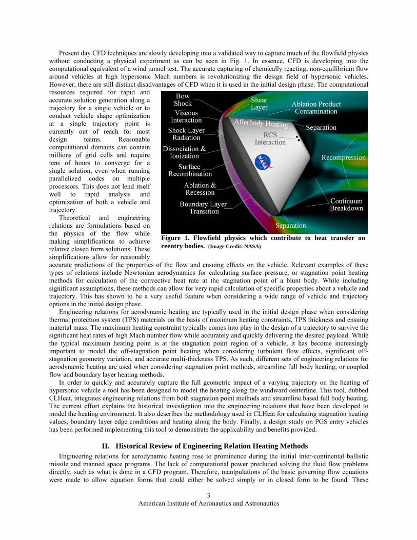
Present day CFD techniques are slowly developing into a validated way to capture much of the flowfield physics without conducting a physical experiment as can be seen in Fig. 1. In essence, CFD is developing into the computational equivalent of a wind tunnel test. The accurate capturing of chemically reacting, non-equilibrium flow around vehicles at high hypersonic Mach numbers is revolutionizing the design field of hypersonic vehicles. However, there are still distinct disadvantages of CFD when it is used in the initial design phase. The computational resources required for rapid and accurate solution generation along a trajectory for a single vehicle or to conduct vehicle shape optimization at a single trajectory point is currently out of reach for most design teams. Reasonable computational domains can contain millions of grid cells and require tens of hours to converge for a single solution, even when running parallelized codes on multiple processors. This does not lend itself well to rapid analysis and optimization of both a vehicle and trajectory.

Theoretical and engineering relations are formulations based on the physics of the flow while making simplifications to achieve relative closed form solutions. These simplifications allow for reasonably accurate predictions of the properties of the flow and ensuing effects on the vehicle. Relevant examples of these types of relations include Newtonian aerodynamics for calculating surface pressure, or stagnation point heating methods for calculation of the convective heat rate at the stagnation point of a blunt body. While including significant assumptions, these methods can allow for very rapid calculation of specific properties about a vehicle and trajectory. This has shown to be a very useful feature when considering a wide range of vehicle and trajectory options in the initial design phase.

Engineering relations for aerodynamic heating are typically used in the initial design phase when considering thermal protection system (TPS) materials on the basis of maximum heating constraints, TPS thickness and ensuing material mass. The maximum heating constraint typically comes into play in the design of a trajectory to survive the significant heat rates of high Mach number flow while accurately and quickly delivering the desired payload. While the typical maximum heating point is at the stagnation point region of a vehicle, it has become increasingly important to model the off-stagnation point heating when considering turbulent flow effects, significant off-stagnation geometry variation, and accurate multi-thickness TPS. As such, different sets of engineering relations for aerodynamic heating are used when considering stagnation point methods, streamline full body heating, or coupled flow and boundary layer heating methods.

In order to quickly and accurately capture the full geometric impact of a varying trajectory on the heating of hypersonic vehicle a tool has been designed to model the heating along the windward centerline. This tool, dubbed CLHeat, integrates engineering relations from both stagnation point methods and streamline based full body heating. The current effort explains the historical investigation into the engineering relations that have been developed to model the heating environment. It also describes the methodology used in CLHeat for calculating stagnation heating values, boundary layer edge conditions and heating along the body. Finally, a design study on PGS entry vehicles has been performed implementing this tool to demonstrate the applicability and benefits provided.

II. Historical Review of Engineering Relation Heating Methods Engineering relations for aerodynamic heating rose to prominence during the initial inter-continental ballistic

missile and manned space programs. The lack of computational power precluded solving the fluid flow problems directly, such as what is done in a CFD program. Therefore, manipulations of the basic governing flow equations were made to allow equation forms that could either be solved simply or in closed form to be found. These

Figure 1. Flowfield physics which contribute to heat transfer on reentry bodies. (Image Credit: NASA)


4

manipulations and simplifications enabled the design of the Mercury, Gemini, and Apollo capsules, the initial design of inter-continental ballistic missiles, and set the stage for the development of the Space Transportation System. Although the advent of CFD has enabled higher fidelity heating solutions to be found, the development of the engineering relations has continued and is still very relevant in the rapid analysis and design phases of a mission. The development of historical stagnation, streamline and flow-boundary layer coupled methods was investigated to allow for the selection of the most relevant methods to be used in the current formulation.

The differing methods under investigation are all attempting to model some aspect of the convective heat transfer over a body in high-speed flow. These types of flow are dominated by the flow features depicted in Fig. 1. The majority of heat transfer is through convective temperature gradients across the boundary layer. Thus in order to calculate the heat transfer rate, information must be known about the temperature at the edge of the boundary layer, on the surface of the body, and the distribution in between. Each of the following methods makes certain steps to simplify the calculation of these values. The challenge of calculating high-speed flow properties is the inability to make generalizing assumptions as is normally done in low speed flow. The high energy and high temperature can lead to dissociation of the gas, boundary layer variations, and increased viscous interaction. Thus the calculation of the heating on bodies in this flow regime is highly dependent on the level of fidelity of the physics of the problem taken into account.

A. Stagnation Point Methods and Distributed Heating Approximations The first engineering methods developed for aerothermodynamic heating were calculations based on the

stagnation region of the vehicle. This allows for the velocity at the edge of the boundary layer to be known by assuming it is zero; however, the remaining gas properties and velocity gradients are still unknown. Work in the 1950s and early 1960s established working relations for total heat transfer as seen in the work of Allen and Eggers1 and instantaneous heat transfer in dissociated air as seen in the work of Fay and Riddell2, Chapman3, and Lees4. This work saw further development to encompass relations for various gas species corresponding to different types of planetary atmospheres by Sutton and Graves5. The dependence on the velocity gradient at the stagnation region was found to be correlated to the physical geometry when the geometry was a spherical forebody. The set of these advancements has led to equations which give a reasonable approximation for the heat rate at the stagnation point of the vehicle, and can be calculated for various vehicle geometries and planets of interest. These equations have also been seen to have a similarity relationship for a hemispherical body in the region near the stagnation point.6 This similarity relationship coupled with the stagnation method can give reasonable values for the distributed heating pattern over a sufficiently blunted vehicle. These relations are still used extensively in current design and analysis work7.

B. Boundary Layer Heating Methods The extension of the analysis beyond the stagnation point also was developed in the mid 1950s. Eckert

developed expressions, including those of a reference enthalpy, for modeling the quantities in the boundary layer of high speed flows8. Concurrently, Lees made similar developments, as for the stagnation point methods, for analyzing heat transfer on blunt bodies4. The advancements in boundary layer development along singular stream lines were made directly relevant to full body analysis due to Cooke’s work on the axisymmetric analogue9. This dictated that flows along a given streamline for an arbitrary body could be treated as being along an equivalent axisymmetric body. These developments set the stage for a large set of further work in 3-D geometry analysis using engineering relations.

The ability to analyze complete geometries using only isolated streamline information set off a major stage of boundary layer and streamline development. A program for calculating the heating distribution over an entire geometry at angle of attack was developed using a conglomeration of the axisymmetric analogue, Lees’ formulations and an approximate technique of streamline distribution by DeJarnette and Davis10. From this point, a diverse set of advancements have been made to advance the fidelity of the calculation of surface streamlines11,12,13, surface pressure13,14,15 and heating formulations13,16,17,18. These advancements have been seen in industry standard codes: HABP19, MINIVER20, AEROHEAT12, INCHES16, CBAERO21, and HATLAP17. These codes have been shown to compare favorably to higher fidelity simulations such as viscous shock layer and CFD22,23,24. Each of these codes is formulated around breaking the flow over the body into individual streamlines based of freestream and geometric configurations and then individually analyzing the properties along each streamline.

Each of these codes uses different types of methods for their heating formulation. One primary method seen in MINIVER and CBAERO is the use of the Reynolds analogy25. The Reynolds analogy stipulates that the heating is directly related to the skin friction. Thus the convective heating on a body can be calculated using previously determined relations for skin friction over a flat plate, with modifications to account for a blunt geometry. This


5

method has significant issues at a stagnation point due to the lack of the typical velocity gradient, even though a significant temperature gradient exists. Another methodology, which can be seen in AEROHEAT, is an equivalent boundary layer method. This is done by directly solving for a unique boundary layer for the given streamline. The integral solution of the boundary layer is highly dependent of the surface and edge quantities, and thus can exhibit higher levels of fidelity depending of the source of the values given. Yet another method is the one used in INCHES, an inviscid flow calculation. This uses an inverse method to simulate the inviscid flow field along the boundary and shock layer. This results in a higher fidelity description of the boundary layer quantities and can integrate more advanced physics, however the complexity and computational resources put this on the fringe of boundary layer methods.

III. Effective Nose Radius Formulation Work conducted by Sutton-Graves and Chapman in the 1950’s and 1960’s established methods for

approximating the heat flux at the stagnation point of a sphere. This work has been applied judiciously to approximate the stagnation point heating of arbitrary bodies while using the radius of curvature at the stagnation point as a baseline value for the developed historical equations. These relations however, were formed under the assumption of a spherical fore-body. It was previously unknown what value to use as the nose radius when a non-spherical body was analyzed. In order to test the applicability of these equations, a comparison with higher fidelity tools has been conducted over a range of free-stream conditions and geometries.

A. Methodology 1. CBAERO Modeling

The Configuration Based Aerodynamics (CBAERO) package developed at NASA Ames was identified as potential tool to handle this task. CBAERO is an advanced panel method analysis tool that is able to couple both modified Newtonian based aerodynamics with approximate post local shock conditions to achieve aerodynamics and aerothermodynamics over arbitrary bodies. The tool has been used extensively21,26 to model complex geometries such as the Space Shuttle, Crew Exploration Vehicle, and HL-20 vehicle, and has been shown to have comparable results to high-fidelity CFD codes. However, the computational speed of the code is multiple orders of magnitude faster than typical CFD codes and can obtain results for a sweep of body geometries and flow conditions within minutes. CBAERO uses a simplified input of Mach number, dynamic pressure, and angle of attack along with a triangulated surface mesh of the body of interest. These values are used in conjunction with the planetary body of interest, vehicle reference values, and turbulence transition criterion. Parametric sweeps of atmospheric and orientation conditions are easily configured to create aerodynamic databases of the geometry. Figure 2 is a view of the typical results for a PGS vehicle after being modeled and run in the CBAERO package.

CBAERO is used in the analysis flow when full body data is desired over a particular geometry. However, for use in an automated fashion rapid design, the calculation time associated with generating the geometry, mesh, and heating profile can be time prohibitive. The calculation of stagnation point heating as done by a simple equation, such as the Chapman or Sutton-Grave equations, is far quicker and of sufficient detail for conceptual studies. The benefit of CBAERO with regards to the current study comes in its ability to compare the stagnation point heating as given by these simple equations with the stagnation point heating as given by a simulation which takes into account the full geometry. In order to compare the results from CBAERO with these simple equations, specifically the Chapman equation, a process has been developed to equate the stagnation point heating values with the effective nose radius.

It was desirable to relate the inputs of CBAERO, Mach number and dynamic pressure, to Chapman's equation. Since Mach number is a function of velocity and temperature, dynamic pressure is a function of density and

Figure 2. CBAERO heating results for a PGS vehicle with calculated streamlines from the stagnation region shown.


6

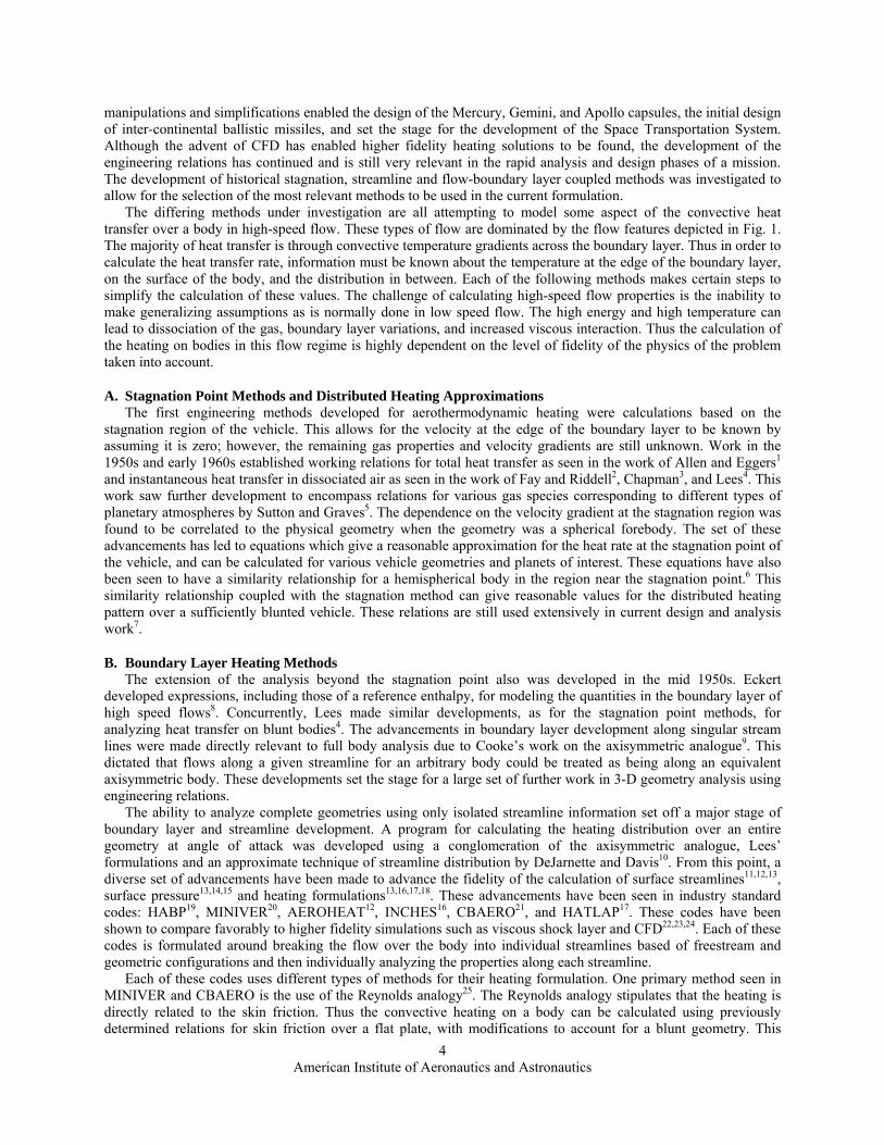
velocity, and Chapman's equation is a function of density and velocity, Chapman's equation was rearranged to be easily determined by CBAERO inputs as shown in Eq. (1) - (6).

15.35.0

8.792417600

⎟⎠⎞⎜

⎝⎛

⎟⎟⎠

⎞⎜⎜⎝

⎛= ∞∞ V

rq

atmn ρρ

& (1)

Chapman’s equation given in Eq. (1) is combined with the Mach number and dynamic pressure relations given in Eq. (2) and (3)

RT

VMγ∞= (2)

2

21

∞∞∞ = Vq ρ (3)

The resulting equation, Eq. (4), is primarily a function of the CBAERO inputs, along with the geometric nose radius, and atmospheric constants.

( )nr

qRTMq ∞

∞=15.2

γα& (4)

( ) atmρ

α 18.7924

21760015.3= (5)

Eq. (6) gives the effective nose radius that results from the application of Chapman’s equation on stagnation point heat fluxes from CBAERO.

( ) 215.2

, ⎟⎟

⎠

⎞

⎜⎜

⎝

⎛= ∞

∞CBAERO

effn qRTM

qr&

γα (6)

In order to correlate the inputs used in CBAERO to the given heat flux, an additional set of relations are solved to rectify the presence of freestream temperature in Eq. (6). First the dynamic pressure equation is combined with a rearranged form of the Mach number equation

RTMq γρ 2

21

=∞ (7)

RM

qT

γρ 2

2∞= (8)

This rearranged form can then be combined with the Ideal gas relation for pressure.

γ

ρ 22M

qRTP ∞== (9)


7

The pressure as a function of altitude is captured by the scale height equation for pressure. The form used in Eq. (10) allows for the piecewise variation of pressure due too the varying temperature gradients in Earth’s atmosphere.

( )

b

bob RT

hhmgPP

−−= exp (10)

( )

⎟⎟⎠

⎞⎜⎜⎝

⎛=

−− ∞

γ21ln 2M

qPRT

hhmg

bb

bo (11)

Thus through final rearrangement, the altitude corresponding to the given Mach number and dynamic pressure can be found.

⎟⎟⎠

⎞⎜⎜⎝

⎛−= ∞

γ21ln 2M

qPg

RThh

bo

bb (12)

Thus, with knowledge of the piecewise temperature dependence on altitude in the Earth’s atmosphere, Eq. (6) can be fully solved for the effective nose radius using only CBAERO inputs and outputs. With this relationship in place, a sweep of Mach numbers, dynamic pressures and angles of attack were run in CBAERO over a sweep of geometries. The results showed a non-constant effective nose radius demonstrating that the use of the physical nose radius did not give an accurate representation of the effective nose radius in the stagnation point heating equation.

2. JMP Curve Fit models

In order to capture the trends observed in the effective nose radius results, the data was analyzed using JMP. JMP is a commercially available data regression and meta-model creation tool. Using this program a multivariable curve fit was created to model the effective nose radius trends. This was conducted by fitting coefficients for a response surface containing variable combinations determined from the anticipated physics of the problem as well as the identified most significant variables. The data from the initial geometry configuration as well as the resulting model can be seen in Fig. 3.

This solution was developed further by investigating the additional geometric dependencies on the stagnation point heat rate. Independent sweeps of geometries which varied the cone angle, base area, or nose radius were conducted. It was found that the effective nose radius relationship was independent of angle of attack, cone angle, and base radius within the ranges modeled. However, there was found to be a significant dependence on the actual nose radius. This dependence was analyzed and a power scaling factor was determined to give the best agreement in the mid-altitude range of flight as can be seen in the leading term of Eq. (13). A plot showing the normalizing ability of this factor is given in Fig. 4 for a wide range of physical nose radii.

B. Resulting Equation and Applicability The resulting equation from the CBAERO modeling leading to the JMP analysis and nose radius correction is

given in Eq. (13). This equation is used to increase the fidelity of the nose radius chosen when analyzing stagnation point heating using either the Chapman or Sutton-Grave equations

⎥⎦

⎤⎢⎣

⎡+−+−−+−

⎟⎟⎠

⎞⎜⎜⎝

⎛=

∞∞

∞∞

)ln(002934.)ln(06076.0)ln(1144.0)...ln(16607.3025757.5288.02335.14244.34

exp2

82.0,

, hqMhqhMhqMqMr

r actneffn

(13)

The benefit of this model is the fidelity of running a CBAERO analysis for a full geometry without the corresponding geometry generation and calculation time. This equation can be implemented anywhere the stagnation point methods are currently being applied and computationally only adds one extra line of computation. Due to the nature of a curve fit relation, the applicability of this equation is only assured within the bounds it was created. The range of applicability is given in Table 1.


8

0

0.5

1

1.5

2

2.5

3

3.5

4

0 10000 20000 30000 40000 50000 60000 70000Altitude, m

Nor

mal

ized

Nos

e R

adiu

s

.5 in1in2in3in4in10in100in

Figure 4. Normalized effective nose radius using a 0.82 normalizing factor to minimize mid-altitude discrepancies

0

2

4

6

8

10

12

14

16

18

20

0 10000 20000 30000 40000 50000 60000

Altitude, m

Rn,

in.

Mach 26Mach 25Mach 24Mach 22Mach 20Mach 16Mach 14Mach 12Mach 10Mach 9.5Model 26Model 25Model 24Model 22Model 20Model 16Model 14Model 12Model 10Model 9.5

Figure 3. JMP curve fit model of effective nose radius as a function of Mach number, dynamic pressure, and altitude for a 2in nose radius sphere cone with varying cone angles.


9

IV. Centerline Heating (CLHeat) Model During the process of design, geometry variations are used to affect the available payload and aerodynamic

performance of a given vehicle. These variations encompass the entire vehicle geometry from fore to aft-body. Stagnation point methods as described in the previous section, can solely account for changes in the nose geometry. In order to capture the full body effect, higher fidelity methods must be employed. Streamline methods are one such means of gaining convective heating information aft of the stagnation point. While some three dimensional engineering codes calculate aerodynamic heating over a body using streamline methods by calculating a full set of approximate streamlines around the body, it is also possible to simplify this calculation by treating the body geometry along the windward centerline as a known streamline. This gives a much less computationally complex calculation scheme while maintaining full geometry calculations. The windward centerline is also typically the highest heating environment on an entry vehicle (can vary due to turbulent heating). This suggests that the calculations for maximum heat rate and thus TPS thickness would be worst case scenarios for the geometry.

The streamline methods are based on the calculation of the boundary layer profile and the resulting fluxes and shear stresses. The streamline along the centerline of the vehicle closely resembles the geometric configuration as seen in Fig. 5. In order to properly calculate the boundary layer quantities used in the centerline heating methodology, it is imperative to accurately calculate the properties at the edge of the boundary layer as well as the surface quantities. This can be achieved using multiple techniques of varying complexity. Inviscid CFD solutions are the highest level of complexity that can be used to calculate the edge conditions. While this can give a mismatch between computational speeds, it can also provide high fidelity heating solutions using the lower fidelity boundary layer methods. To match the computational speed and accuracy of the edge conditions with the boundary layer equations, it is typical to use body geometry based methods, such as Newtonian based pressure coefficients. This aligns with the type of fidelity used in conceptual design and maintains rapid computational speed. Note that a benefit of the streamline method described below is the ability to use higher fidelity edge conditions if they are available.

A. Methodology 1. Edge Condition Formulation

The conditions of interest at the edge of the boundary layer are pressure, density, velocity, and Mach number. In order to determine these quantities from the freestream Mach number, freestream dynamic pressure, and body geometry, the following methods were derived. Note that these inputs are consistent with industry codes for comparison, and can be easily derived from trajectory propagation.

The freestream pressure is derived from the Ideal gas law, Mach number definition and dynamic pressure equation as seen in Eq. (9). The freestream total temperature and associated specific heat and specific heat ratio are

Table 1. Effective Nose Radius Range of Applicability

Figure 5. Streamline methods and edge conditions based on normal shock entropy and geometry based streamline shape12


10

determined by a rapid iterative process involving an update of the specific heat ratio, γ, based on the total temperature of the flow. This process involving Eq. (14)-(18) is repeated until converged total temperature and gas properties are found. The use of temperature dependent specific heats leads to a total temperature calculation that is up to 30 percent more accurate than using fixed values.

∞

∞∞ =

RTP

ρ (14)

∞∞∞ = ρ/2qV (15)

AIRpC

VTT 22

0∞

∞ += (16)

))(),(( 00 22TCTCfC

NOAIR ppp = (17)

( )RCC

AIR

AIR

p

p−=∞γ (18)

After finding the total temperature and gas properties in the freestream, the post shock and local edge conditions are calculated. The total freestream pressure is found using isentropic relations:

120 2

11

−

∞∞

∞

∞

∞

∞⎟⎠

⎞⎜⎝

⎛ −+=

γγ

γMPP (19)

This is used with Eq. (20) to find the total pressure post-shock using the formula for total pressure change across a normal shock. Note that this assumes a normal shock is the predominant flow feature. This is characteristically true for boundary layer calculations as the streamlines in the boundary layer are the stream lines closest to the stagnation streamline which will always pass through a normal shock if the shock is detached.

( )( )( )

( )( )

11

2

1

2

2

00 121

121

1

−

∞∞∞

∞−

∞∞

∞∞∞∞

∞

∞ ⎟⎟⎠

⎞⎜⎜⎝

⎛

−−+

⎟⎟⎠

⎞⎜⎜⎝

⎛

−++

=γγ

γ

γγγ

γγ

MMM

PP (20)

The pressure at the edge of the boundary layer is then calculated using the pressure coefficient from Newtonian theory and the stagnation pressure from Eq. (20).

⎟⎟⎠

⎞⎜⎜⎝

⎛+= ∞∞

21

2

01

MCPP press

edge

γ (21)

The edge Mach number is calculated from the isentropic pressure ratio of the edge pressure to total post shock pressure, and is thus a calculation of the flow expansion from the stagnation region. This methodology is repeated for the edge temperature as well.

( ) ⎟⎟⎠

⎞⎜⎜⎝

⎛−

⎟⎠⎞

⎜⎝⎛ −=

∞

−

∞

∞

121/

1

01 γγγ

edgeedge PPM (22)


11

2

0

21

1 edge

edge

M

TT

−+

=∞γ

(23)

Finally, the edge velocity is calculated from the local Mach number and speed of sound.

edgeedgeedge RTMV γ= (24)

It should be noted that any mix of available data can be used in this calculation to increase the fidelity of the edge predictions, including exact freestream temperature, equilibrium air composition, or surface pressure distribution.

2. Streamline Heating Equations and Applicability

The calculation of the convective heating along a streamline is governed by not only the prediction of the edge conditions, but also the accurate application of Reynolds analogy for a compressible boundary layer. The method used for the current effort was first described by Zoby, Moss, and Sutton18. Minor modifications have been made to make use of the most recent understanding of boundary layer theory and parameter estimation. These equations can be held valid in a supersonic flow when there is no static pressure gradient across the boundary layer. This is a good assumption for most boundary layers except those where entropy layer swallowing takes place. Entropy layer swallowing can occur at high Mach numbers when both the entropy layer and boundary layer are significantly large. In order to predict when this swallowing takes place, higher fidelity methods than what is currently being presented must be used. The laminar boundary layer method is presented below and the turbulent boundary method is presented in the Appendix.

The convective heating equation found in Eq. (31) is a modified Blasius boundary layer equation using Reynolds analogy for the skin friction to heat rate comparison. The compressibility effects are integrated using a reference enthalpy approach. The Meador-Smart reference temperature is given in Eq. (25). All star values shown herein are calculated using the temperature from this formula.

⎟⎟⎠

⎞⎜⎜⎝

⎛ −++=∗ 2

21Pr16.055.045.0 edge

edge

walledge M

TT

TT γ (25)

Sutherland’s viscosity law is used in order to account for temperature varying viscosity using standard temperature and pressure as the reference value.

110110

5.1

++

⎟⎟⎠

⎞⎜⎜⎝

⎛=

TT

TT ref

refrefμμ (26)

Enthalpies are calculated using the constant specific heat calculated in the edge conditions and with a constant Prandtl number.

2

2Pr

edgeedgepaw VTCHAIR

+= (27)

wallpwall TCHAIR

= (28)

Figure 6. Variable nomenclature for the streamline heating calculation.


12

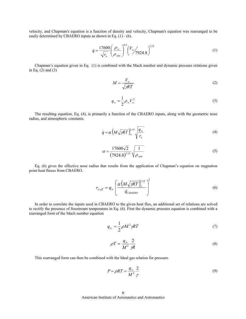
The momentum boundary layer thickness is used in the calculation of Reynolds number. This momentum boundary layer thickness, Eq. (30), is the main location where the basic equations vary from the flat plate solution. In the current method, the distance along the streamline is given as the distance along the body from the stagnation point, and the radius is the current body radius at the given point as seen in Fig. 6.

edge

LedgeedgeVμ

θρθ =Re (29)

⎟⎟⎟⎟⎟

⎠

⎞

⎜⎜⎜⎜⎜

⎝

⎛

=∫ ∗∗

rV

dsrV

edgeedge

S

edge

L ρ

μρθ 0

2

664.0 (30)

The use of these equations leads to the calculation of the convective heat rate at the given location and edge conditions. As this is an integral method, all points prior to the location of interest must be analyzed in order for a solution to be found.

edgeedge

waw

edgeedgelam VHHq ρ

μμ

ρρ

θ6.0PrRe

22.0 −=

∗∗

& (31)

The wall temperature is calculated in two manners, constant or radiative equilibrium. In order to calculate the radiative equilibrium solution, the previous method is solved such that the wall temperature and the final heat flux determined wall temperature as shown in Eq. (32) are in alignment.

25.0

⎟⎠⎞

⎜⎝⎛=εσqTwall& (32)

A similar process can be followed for calculating the turbulent heating solution and can be found in the Appendix. The solution can be given as fully turbulent, fully laminar or transitional. The transition model is based off a user defined value of momentum thickness Reynolds number at which transition occurs. The transition region is defined as linearly weighted average of the laminar and turbulent heating values; the length used in the weighting is the length of the laminar region from the stagnation point to the transition location.

3. Multi-Method Integration

The streamline boundary layer method developed is inherently invalid at the stagnation point. In order to accurately predict the heating over all regions of the body, a mix of methods is employed. Stagnation point methods using the effective nose radius value as previously presented and in Eq. (33), are used to calculate the heat rate at the nose and just off the stagnation point a variant of the Fay-Riddell equation is used as seen in Eq. (34).

15.3

5.0

,

Vr

kqeffn

stag ⎟⎟⎠

⎞⎜⎜⎝

⎛=

ρ& (33)

( )dxdUHHq edgeedgewawdxdu μρ−= 6.0/ Pr

763.0& (34)

Equation (34) is then averaged into the streamline method given in Eq. (31) for laminar flow or the equivalent for turbulent flow. The exact location of method transition is given by the relative magnitude of the modes in comparison and the relative location of applicability of the method in order to maintain a conservative estimate of the heat rate along the body.


13

B. Validation of Edge Conditions and CLHeat Implementation In order to confirm that the edge condition formulation is consistent with other industry standard tools, a

comparison was conducted with CBAERO. Various geometries and flow conditions were analyzed using both CLHeat and CBAERO and the resulting edge conditions as a function of the pressure coefficient were compared. By comparing to the pressure coefficient multiple details could be verified. Due to the use of modified Newtonian aerodynamics for the pressure distribution and maximum pressure, a verification that the correct specific heat ratio was found for the given freestream Mach and dynamic pressure is performed by checking the maximum pressure coefficient. The comparison plots of the remaining edge conditions can be seen in Fig. 7. As shown, the edge Mach number, pressure, and velocity all compare very favorably with CBAERO. Edge temperature has a significant offset. This is due to the difference in the composition calculation between CBAERO and CLHeat. CBAERO calculates equilibrium air at all times using curve fit tables. CLHeat currently uses a frozen composition of oxygen and nitrogen. This difference predictably leads to a higher edge temperature in CLHeat than in CBAERO as CLHeat is using fewer degrees of freedom for the energy modes.

Figure 7a. Edge condition validation against CBAERO results for boundary layer edge pressure, Mach.

Figure 7b. Edge condition validation against CBAERO results for boundary layer edge velocity, and temperature.


14

The validation of CLHeat against CBAERO for a full geometry can be seen in Figures 8 and 9. Figure 8 is the comparison of a 60 degree sphere cone with 1m nose radius in both CBAERO and CLHeat. The overall trend between the two models is very similar and in some regions nearly exact. However obvious differences clearly occur. The stagnation region modeled in CLHeat shows a drastic offset followed by a step increase until the models align. This is due to the multi-method integration in CLHeat to account for the stagnation offset. The flat region near x=0.2 is also an artifact of the method transition. The peak magnitudes and overall trends seem to show very strong agreement and the decreasing trend seen in contrast to CBAERO for x>0.8 is what should be expected due to laminar flow theory. Figure 9 compares the heating distribution over a Bezier curve of revolution27. The trends between CBAERO and CLHeat are very comparable with CLHeat projecting a higher stagnation value but lower heating as the flow progress towards the aft of the vehicle. Finally, Figure 10 shows a comparison of the CLHeat modeling of both the laminar and turbulent formulations against data from Zoby, Moss and Sutton18. This is a model of a 40 degree sphere cone with 0.3048 m radius nose in Mach 10 flow. The results give increased confidence in the implementation of the current formulation for the assumptions made. Although CLHeat uses a different formulation for the edge conditions, reference enthalpy, and flow chemistry than the tabulated data, the trends and values show very close alignment for both the laminar and turbulent cases.

These validation cases show favorable results that the CLHeat tool is representing the heating along the body of arbitrary entry geometries in a manner consistent with the fidelity provided by tools such as CBAERO. The lack of perfect agreement may be attributable to multiple factors, but the agreement on trends and magnitude suggests that the proper physics is being considered. There is also no expectation that perfect agreement with a tool such as CBAERO can be achieved. The modeling features of CBAERO are currently unknown by the authors, and as such any inconsistencies do not have a directly attributable cause. While certain assumption such as frozen flow and radiative equilibrium may not apply for all cases, CLHeat allows for the ability to modify the given assumptions to better represent the flow features at hand.

X, X,m

Qdo

t(W

/m2)

0 0.5 1 1.5 20

100000

200000

300000

400000 QdotFinCBAERO

Figure 8. CLHeat comparison with CBAERO for a 60 degree sphere cone at Mach 12. Geometry in inset figure.

X

CLHeat CBAERO

0 1 20

1

2

3

4


15

V. Design Study Utilizing Centerline Heating Model The ability to model the heating along a body in a rapid manner can pay great dividends in the conceptual design

phase of a hypersonic vehicle. In order to effectively design and optimize a vehicle, a wide range of vehicles must

X

Qdo

t(W

/m2)

0 0.2 0.4 0.6 0.8 1

500000

1E+06

1.5E+06

2E+06

2.5E+06

3E+06

3.5E+06

4E+06

4.5E+06

QdotFinCBAERO

Figure 9. CLHeat comparison with CBAERO for a Bezier curve at Mach 9 with a dynamic pressure of 2.2MPa. Geometry in inset figure.

X

Qdo

t,W

/m^2

0 0.5 1 1.5 2 2.5 30

500000

1E+06

1.5E+06

2E+06

2.5E+06

3E+06

3.5E+06

Qdot LamQdot TurbExp LamExp Turb

Figure 10. Validation of CLHeat modeling of both the laminar and turbulent formulation against data from Zoby, Moss, Sutton18

CLHeat CBAERO

0 0.5 10

0.1

0.2


16

be analyzed in conjunction with the constraints and performance metrics for the mission at hand. The wider the design space available, the more likely the best design can be found. However in order to have a wide design space, the speed of the analysis tools must conform with the number of cases desired to be run and the total amount of time available. The CLHeat tool is nearly computationally transparent with respect to the time needed to fully propagate a trajectory or run TPS thickness sizing. As such a significant advance in the heating knowledge can be given to conceptual vehicle designers without a significant increase in simulation time or decrease of the design space.

The best use of the CLHeat tool in design studies is to locate maximum heat rate locations for TPS material selection or constraint verification, to identify trajectories that exhibit turbulent flow onset, or to calculate the distributed heating patterns for linkage with a TPS thickness sizing tool. The speed of the tool also allows for the constraint verification to be achieved on the fly during trajectory propagation for use in optimization methods. This can be a significant improvement over stagnation based methods when flight regimes or vehicle geometries cause the maximum heat rate location to be off-stagnation.

In order to demonstrate the use of the CLHeat tool in a design study, an integrated trajectory and vehicle optimization study for PGS missions has been conducted.

A. Prompt Global Strike Mission Overview The PGS mission objective is to be able to deliver conventional weapons accurately and rapidly in a global

arena. In order to do this the weapon system must reliably be able to travel vast ranges with significant control authority while maintaining a significant payload. The acquisition of this type of capability allows for a response to critical threats without having to resort to the use of the nuclear option or having a wide deployment of personnel. In order to design such a system, both the launch and entry phases must be considered. The current study considers the design of an entry body when the total length of the booster and entry body is limited. This limitation dictates that different length and weight entry vehicle options correspond to varying initial conditions for the entry phase. This matching of initial conditions to a given entry vehicle class can be seen in Table 2.

The study considers the optimal sweep of vehicles for each entry class of entry vehicle and initial condition

given in Table 2. The optimal sweep is defined by the typically conflicting goals of maximum range and effective maximum volume. The heating considerations as given by CLHeat include the maximum heat rate constraints for ablative TPS and the volume and useful payload mass penalties for the associated TPS thickness to withstand the heating environment.

B. Design Study Models 1. Particle Swarm and Pareto Front Optimization

The design study framework is based around a particle swarm optimization process for both the body dimensions and the angle of attack profile. Each individual particle within the optimization process holds an unique vehicle shape and corresponding trajectory inputs. Each particle is then used as the initial conditions for the trajectory simulation; the resulting performance metrics are calculated and shared with the other particles to help drive the set of particles to the optimal values. The optimal values are considered the points that are uniquely optimal for both downrange and useful volume. These points are considered to lie along the Pareto front, as they form a set of points of which no performance gain can be achieved in one metric without a corresponding change in the alternate metric. The integrated trajectory tool, particle swarm technique, and Pareto front optimization has been previous applied to Mars entry simulations and shown to give designers an increased understanding of multi-disciplinary design decisions28.

Table 2. PGS design study vehicle constraints and initial conditions Glide

Vehicle Mass (lb)

Glide Vehicle Length (in)

Glide Vehicle Diameter (in)

Reentry Gamma (deg)

Reentry Velocity(ft/sec)

325 48 18 -20.1 10419

325 48 18 0 10092

250 45 15 -25 12269

250 45 15 0 11689

Glide Vehicle

Mass (lb)

Glide Vehicle Length (in)

Glide Vehicle Diameter (in)

Reentry Gamma (deg)

Reentry Velocity(ft/sec)

325 48 18 -20.1 10419

325 48 18 0 10092

250 45 15 -25 12269

250 45 15 0 11689


17

2. Aerodynamic Module The geometry configurations used in the current design study are blunt Bezier curves of revolution. These

geometries are characterized by a smooth profile from nose to tail rotated around the axis of symmetry. The given Bezier curves can be configured according to three parameters which effect overall bluntness, length and diameter. Previous efforts by Grant29 have led to analytic formulas for the calculation of Newtonian Aerodynamic based lift, drag, moment, and stability coefficients for various geometries, including Bezier curves of revolution. This capability allows for very rapid calculation of the needed trajectory propagation inputs for the wide range of geometries considered within the study.

3. TPS sizing

The calculation of effective volume is conducted by subtracting the necessary TPS volume from the volume constrained by the outer mold line. This method is used due to the stipulation of a fixed entry mass instead of a fixed density. In order to calculate the TPS volume, a distributed TPS thickness is calculated over the body. This calculation is performed by integrating the one-dimensional heat conduction equations over the entire trajectory using surface the radiative equilibrium surface temperature calculated from the heat flux. To achieve the more accurate prediction of the total TPS thickness over the body, the CLHeat tool is used at each trajectory point to calculate the heat flux and associated surface temperature. Multiple points across each body are tracked, as well as the point of maximum heat flux, and the TPS thickness is calculated at each of these points. Overall volume TPS volume is then calculated by projecting the calculated thickness from the calculation point to the next point downstream. The thickness is then integrated around the body to calculate the total volume. The thickness sizing for the current study is done to limit the TPS bondline temperature to 250 deg Celsius assuming a carbon-phenolic TPS is used. This method gives a more accurate, but still conservative, value for the distributed thickness by allowing for diminishing thickness along the body but still ensuring the thickness in a given region is calculated at its maximum value.

C. Design Study Results and Trends To create the Pareto fronts of optimal results of maximum downrange and effective volume, 50 particles are run

for 50 iterations within the particle swarm optimization process. This creates a Pareto front consisting of 50 unique vehicle and trajectory configurations. Each simulation is run twice for the same initial conditions once with and once without the heating and TPS sizing constraints. This allows for a clear comparison of the benefits of including heating in the loop of the optimization process.

The primary results can be seen in Fig. 11 and 12. Figure 11 depicts the resulting Pareto frontier between maximizing effective entry volume and maximizing downrange. Of key interest is the difference between the solutions utilizing TPS sizing for the calculation of effective volume, shown in blue, and those neglecting TPS volume, shown in red). The lower downrange solution show a constant drop between the two curves, however, there is a critical point of deviation near a downrange of 1200 km. Similar critical points can be seen in Figure 12. The effect of the variation between the two Pareto fronts is best seen in the differences of geometry for similar performance metrics. The blue and red asterisks in Fig. 11a correspond to geometries of equivalent effective volume. There is a nearly 200 km difference in the downrange between these geometries. This is mainly attributed to the blunter geometry needed for the TPS affected geometry to have the same internal volume as the geometry without a TPS as can be seen in Fig. 11b. This blunting effect leads to a lower lift to drag ratio at angle of attack, and thus a shorter trajectory.

A major point of interest is the difference between the red and green asterisks and corresponding geometries. These vehicle and trajectory points correspond to the same downrange, but surprisingly have vastly different geometries. This shows the vast benefit of including the TPS sizing in the loop of the optimization process. If the TPS volume was solely taken as a penalty applied after the optimization had been considered, then the geometries would have been identical between the points of equal downrange; however, the different geometries demonstrates that the optimization process is able to find the balancing optimum between vehicle shape and trajectory to maximize the effective volume. Traditional design studies would thus choose a larger overall vehicle and end up paying the penalty of exceeding the heating constraints by having to apply too much TPS than would be required on a more aptly designed vehicle. This also identifies interesting trends in long down range vehicles that need to be considered when performing mission selection.


18

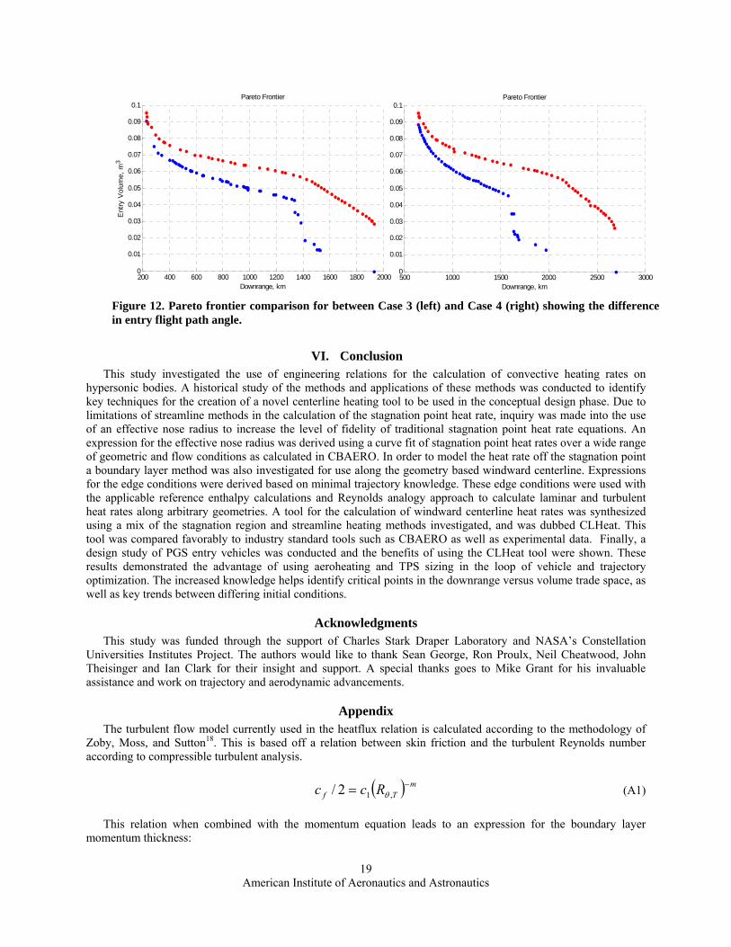
Another trend of interest is shown in the difference between the Pareto frontier plots of identically constrained

geometries with differing initial conditions. Case 3 and 4 shown in Table 2 differ primarily in the initial flight path angles of -25.0 and 0.0 degrees, respectively. With similar entry velocities it is expected that the shallower initial flight path angle would be able to fly a longer trajectory for an identical geometry, and this is confirmed in Fig. 12. The maximum downrange is nearly 800 km further for the shallower flight path angle when considering the non-TPS affected Pareto fronts. This difference is minimized when the distributed heating and TPS sizing is taken into account. The maximum downrange with a non-zero volume is approximately 500 km different, and the difference in the critical point where TPS sizing has its largest effect is only 200 km. The critical point is also found at approximately the same effective volume for both cases.

The results given in this design study show trends that highlight the importance of including TPS sizing in the optimization loop. The behavior of optimal vehicles and trajectories at large down ranges is highly dependent on the heating effects. Neglecting the heating effects or applying them after the initial optimization process can affect the major trends of the design. This also highlights the need to include better fidelity heating models within the optimization as important flow characteristics, such as turbulence or off-stagnation maximum heating points could impact the trends in the design.

0 0.5 1 1.5-0.5

-0.4

-0.3

-0.2

-0.1

0

0.1

0.2

0.3

0.4

0.5

x, m

r, m

Vehicle Shape

200 400 600 800 1000 1200 1400 1600 18000

0.02

0.04

0.06

0.08

0.1

0.12

0.14

0.16

Downrange, km

Ent

ry V

olum

e, m

3

Pareto Frontier

Figure 11. a) Pareto Frontier for Case 1 showing TPS based optimization in red, and trajectory and vehicle only in blue. b) Vehicle geometries at color specified points of interest; blue and red correspond to equivalent effective volume, red and green correspond to equivalent downrange.


19

VI. Conclusion This study investigated the use of engineering relations for the calculation of convective heating rates on

hypersonic bodies. A historical study of the methods and applications of these methods was conducted to identify key techniques for the creation of a novel centerline heating tool to be used in the conceptual design phase. Due to limitations of streamline methods in the calculation of the stagnation point heat rate, inquiry was made into the use of an effective nose radius to increase the level of fidelity of traditional stagnation point heat rate equations. An expression for the effective nose radius was derived using a curve fit of stagnation point heat rates over a wide range of geometric and flow conditions as calculated in CBAERO. In order to model the heat rate off the stagnation point a boundary layer method was also investigated for use along the geometry based windward centerline. Expressions for the edge conditions were derived based on minimal trajectory knowledge. These edge conditions were used with the applicable reference enthalpy calculations and Reynolds analogy approach to calculate laminar and turbulent heat rates along arbitrary geometries. A tool for the calculation of windward centerline heat rates was synthesized using a mix of the stagnation region and streamline heating methods investigated, and was dubbed CLHeat. This tool was compared favorably to industry standard tools such as CBAERO as well as experimental data. Finally, a design study of PGS entry vehicles was conducted and the benefits of using the CLHeat tool were shown. These results demonstrated the advantage of using aeroheating and TPS sizing in the loop of vehicle and trajectory optimization. The increased knowledge helps identify critical points in the downrange versus volume trade space, as well as key trends between differing initial conditions.

Acknowledgments This study was funded through the support of Charles Stark Draper Laboratory and NASA’s Constellation

Universities Institutes Project. The authors would like to thank Sean George, Ron Proulx, Neil Cheatwood, John Theisinger and Ian Clark for their insight and support. A special thanks goes to Mike Grant for his invaluable assistance and work on trajectory and aerodynamic advancements.

Appendix The turbulent flow model currently used in the heatflux relation is calculated according to the methodology of

Zoby, Moss, and Sutton18. This is based off a relation between skin friction and the turbulent Reynolds number according to compressible turbulent analysis.

( ) mTf Rcc −= ,12/ θ (A1)

This relation when combined with the momentum equation leads to an expression for the boundary layer momentum thickness:

200 400 600 800 1000 1200 1400 1600 1800 20000

0.01

0.02

0.03

0.04

0.05

0.06

0.07

0.08

0.09

0.1

Downrange, km

Ent

ry V

olum

e, m

3

Pareto Frontier

500 1000 1500 2000 2500 30000

0.01

0.02

0.03

0.04

0.05

0.06

0.07

0.08

0.09

0.1

Downrange, km

Pareto Frontier

Figure 12. Pareto frontier comparison for between Case 3 (left) and Case 4 (right) showing the difference in entry flight path angle.


20

( )rudSruc ee

cscm

eT ρμρθ4

3

0

**2 ⎟⎟

⎠

⎞⎜⎜⎝

⎛= ∫ (A2)

The c and m terms are based of a relation to the compressible factor, N. A curve fit of N based on experimental data gives the following expression,

( ) ( )( )2,10,10 log21.1log5.667.12 TT RRN θθ +−= (A3)

This corresponds to the m and c values as follows,

( )12 += Nm (A4)

( ) ( )( )( )[ ]mmN NNNcc 211 51 ++= (A5)

( ) 12 1 cmc += (A6)

mc += 13 (A7)

34 /1 cc = (A8)

Nc 93.02433.25 += (A9)

These values are then used to calculate the turbulent heat flux using the edge and reference conditions previous calculated in a similar manner to Eq. (31).

( ) ( )( ) ( )( ) 4.0**,1, Pr −− −= wwawee

mee

mTTw HHuRcq ρμμρρθ& (A10)


21

References

1 Allen, J. and Eggers, A.J. Jr., “A Study of the Motion and Aerodynamic Heating of Ballistic Missiles Entering the Earth’s Atmosphere as High Supersonic Speeds” NACA Report 1381.1958.

2 Fay, J.A. and Riddell, F.R., "Theory of Stagnation Point Heat Transfer in Dissociated Air, Journal of the Aeronautical Sciences, Vol. 121, No. 25, 1958, pp. 73-85.

3 Chapman, G.T., “Theoretical Laminar Convective Heat Transfer and Boundary-Layer Characteristics on Cones at Speeds to 24 km/sec” NASA TN D-2463, 1964.

4 Lees, L., "Laminar Heat Transfer Over Blunt-Nosed Bodies at Hypersonic Flight Speeds," Jet Propulsion, Vol. 26, No. 4, April 1956, pp. 259-269, 274.

5 Sutton, K. and Graves, R.A. Jr., "A General Stagnation-Point Convective-Heating Equation for Arbitrary Gas Mixtures," NASA TR R-376, 1971.

6 Tauber, M.E., “A Review of High-Speed Convective, Heat-Transfer Computation Methods” NASA TP-2914, 1989. 7 Anderson, J.D., Jr., “A Survey of Modern Research in Hypersonic Aerodynamics” AIAA-84-1578, 17th Fluid Dynamics,

Plasma Dynamics, and Lasers Conference. Snowmass, Colorado, June 25-27, 1984. 8 Eckert, E.R.G., “Engineering Relations for Friction and Heat Transfer to Surfaces in High Velocity Flow” Journal of

Aeronautical Science. Vol. 22 No.8, 1955, pp. 585-587. 9 Cooke, J. C., “An Axially Symmetric Analogue For General Three-Dimensional Boundary Layers,” British Aeronautical

Research Council, Rept. and Memorandum No. 3200, London, 1961. 10 DeJarnette, F. R., and Davis, R. M., “A Simplified Method of Calculating Laminar Heat Transfer over Bodies at an Angle

of Attack,” NASA TN-4720, Aug. 1968. 11 DeJarnette, F. R., and Hamilton, H. H., "Inviscid Surface Streamlines and Heat Transfer on Shuttle-Type Configurations,"

Journal of Spacecraft and Rockets, Vol. 10, No. 5, 1973, pp. 314-321. 12 Riley, C. J., DeJarnette, F. R., and Zoby, E. V., "Surface Pressure and Streamline Effects on Laminar Heating

Calculations," Journal of Spacecraft and Rockets, Vol. 27, No. 1, 1990, pp. 9-14. 13 Riley, C.J., DeJarnette, F.R., “Engineering Aerodynamic Heating Method for Hypersonic Flow” Journal of Spacecraft and

Rockets, Vol. 29, No. 3, 1992, pp. 327-334. 14 Hassan, B., DeJarnette, F. R., and Zoby, E. V., “Effect of Nose Shape on Three-Dimensional Streamlines and Heating

Rates” Journal of Spacecraft and Rockets, Vol. 30, No. 1, 1993, pp. 69-78. 15 Maslen, S. H., “Inviscid Hypersonic Flow past Smooth Symmetric Bodies,” AIAA Journal, Vol. 2, No. 6, 1964, pp. 1055–

1061. 16 Zoby, E.V., and Simmonds, A. L., “Engineering Flowfield Method with Angle-of-Attack Applications,” Journal of

Spacecraft and Rockets, Vol. 22, No. 4, 1985, pp. 398–404. 17 Jain, A.C., Hayes, J.R., “Hypersonic Pressure, Skin-Friction, and Heat Transfer Distributions on Space Vehicles: Planar

Bodies” AIAA Journal Vol. 42 No. 10, October 2004, pp. 2060-2068. 18 Zoby, E. V., Moss, J. N., and Sutton, K., "Approximate Convective Heating Equations for Hypersonic Flows," Journal of

Spacecraft and Rockets, Vol. 18, No. 1, 1981, pp. 64-70. 19 Smyth, D. N. and Loo, H. C., “Analysis of Static Pressure Data from 1/12-scale Model of the YF-12A. Volume 3: The

MARK IVS Supersonic-Hypersonic Arbitrary Body Program, User's Manual,” NASA-CR-151940, Oct. 1981. 20 "A Miniature Version of the JA70 Aerodynamic Heating Computer Program H800 (MINIVER)," MDC 60642, revised

Jan. 1972. 21 Kinney, D. J., “Aero-Thermodynamics for Conceptual Design” AIAA-2004-31-962, 42nd AIAA Aerospace Sciences

Meeting and Exhibit, Reno, NV, 5-8 Jan. 2004. 22 DeJarnette, F.R., Hamilton, H.H., Weilmuenster, K.J., Cheatwood, F.M., “ A Review of Some Approximate Methods Used

in Aerodynamic Heating Analyses” Journal of Thermophysics. Vol. 1, No. 1, January 1987. pp. 5-12. 23 Thompson, R.A., Zoby, E.V., Wurster, K.E., Gnoffo, P.A., “Aerothermodynamic Study of Slender Conical Vehicles”

Journal of Thermophysics. Vol. 3 No. 4. October 1989, pp. 361-367. 24 Wurster, K., Zoby, E., and Thompson, R., “Influence of Flow Field and Vehicle Parameters on Engineering Aerothermal

Methods,” AIAA Paper 89-1769, June 1989. 25 Anderson, J.D., Fundamentals of Aerodynamics 3rd. Edition, McGraw-Hill, 2001. 26 Kinney, D.J., Garcia, J.A., Huynh, L. “Predicted Convective and Radiative Aerothermodynamic Environments for Various

Reentry Vehicles Using CBAERO” AIAA-2006-659, 44th AIAA Aerospace Sciences Meeting and Exhibit, Reno, NV, 9-12 Jan. 2006.

27 Rogers, D. F., An Introduction to NURBS: With Historical Perspective, Academic Press, London, 2001. 28 Grant, M. J. and Mendeck, G. F., “Mars Science Laboratory Entry Optimization Using Particle Swarm Methodology,"

AIAA 2007-6393, AIAA Atmospheric Flight Mechanics Conference and Exhibit, Hilton Head, SC, 20-23 Aug. 2007. 29 Grant, M.J., Braun, R.D. “Analytic Hypersonic Aerodynamics for Conceptual Design of Entry Vehicles” AIAA 2010-

1212, 48th AIAA Aerospace Sciences Meeting Including the New Horizons Forum and Aerospace Exposition Orlando, FL, 4 - 7 January 2010.

centerline heating methodology for use in preliminary ... · centerline heating methodology for use...

Documents