central limit theorem for biased random walk on multi-type...

E l e c t r o n ic

Jo

ur n a l

of

Pr

o b a b i l i t y

Electron. J. Probab. 0 (2012), no. 0, 1–40.ISSN: 1083-6489 DOI: 10.1214/EJP.vVOL-PID

Central limit theorem for biased random walkon multi-type Galton–Watson trees

Amir Dembo∗ Nike Sun†

Abstract

Let T be a rooted supercritical multi-type Galton–Watson (MGW) tree with types com-ing from a finite alphabet, conditioned to non-extinction. The λ-biased random walk(Xt)t≥0 on T is the nearest-neighbor random walk which, when at a vertex v withdv offspring, moves closer to the root with probability λ/(λ+ dv), and to each of theoffspring with probability 1/(λ + dv). This walk is recurrent for λ ≥ ρ and transientfor 0 ≤ λ < ρ, with ρ the Perron–Frobenius eigenvalue for the (assumed) irreduciblematrix of expected offspring numbers. Subject to finite moments of order p > 4 forthe offspring distributions, we prove the following quenched CLT for λ-biased randomwalk at the critical value λ = ρ: for almost every T, the process |Xbntc|/

√n converges

in law as n → ∞ to a reflected Brownian motion rescaled by an explicit constant.This result was proved under some stronger assumptions by Peres–Zeitouni (2008)for single-type Galton–Watson trees. Following their approach, our proof is based ona new explicit description of a reversing measure for the walk from the point of viewof the particle (generalizing the measure constructed in the single-type setting byPeres–Zeitouni), and the construction of appropriate harmonic coordinates. In carry-ing out this program we prove moment and conductance estimates for MGW trees,which may be of independent interest. In addition, we extend our construction ofthe reversing measure to a biased random walk with random environment (RWRE)on MGW trees, again at a critical value of the bias. We compare this result against atransience–recurrence criterion for the RWRE generalizing a result of Faraud (2011)for Galton–Watson trees.

Keywords: Multi-type Galton–Watson tree; biased random walk; central limit theorem; random

walk with random environment.AMS 2010 Subject Classification: Primary 60F05; 60K37, Secondary 60J80; 60G50.

Submitted to EJP on November 18, 2010, final version accepted on August 24, 2012.Supersedes arXiv:1011.4056.

∗Departments of Mathematics and Statistics, Stanford University, USA. E-mail: [email protected].†Department of Statistics, Stanford University, USA. E-mail: [email protected].

http://ejp.ejpecp.org/

http://dx.doi.org/10.1214/EJP.vVOL-PID

http://arXiv.org/abs/1011.4056

2 CLT for biased random walk on multi-type Galton–Watson trees

1 Introduction

Let T denote an infinite tree with root o. The λ-biased random walk on T, hereafterdenoted RWλ(T), is the Markov chain (Xt)t≥0 with X0 = o such that given Xt = v withoffspring number dv and v 6= o, Xt+1 equals the parent of v with probability λ/(λ+ dv),and is uniformly distributed among the offspring of v otherwise (and if Xt = o, thenXt+1 is uniformly distributed among the offspring of o).

For supercritical Galton–Watson trees without leaves, if ρ denotes the mean offspringnumber, then RWλ is a.s. recurrent if and only if λ ≥ ρ ([25, Thm. 4.3 and Propn. 6.4]),and ergodic if and only if λ > ρ ([20, Propn. 9-131] and [25, p. 944 and p. 954]). With|v| denoting the (graph) distance from vertex v to the root o, |Xt|/t converges a.s. toa speed V , with V = V (λ) deterministic, positive for λ < ρ and zero otherwise (see[27, 28] for λ < ρ and [32] for λ = ρ; the case λ > ρ follows trivially from positiverecurrence).

Further, subject to no leaves and finite exponential moments for the offspring dis-tribution, a quenched CLT for RWλ (λ ≤ ρ) on single-type Galton–Watson trees wasshown by Peres–Zeitouni [32], and extended to the setting of random walk with ran-dom environment (RWRE) by Faraud [13]. In contrast, if leaves occur, there emerges azero-speed transient regime λ < λc (for λc < ρ) [28] where the leaves “trap” the randomwalk and create slow-down. It follows from the results of Ben Arous et al. [3] that in thissetting, for sufficiently small λ there cannot be a (functional) CLT with diffusive scaling.Analogous results on the critical (ρ = 1) Galton–Watson tree conditioned to survive wereshown by Croydon et al. [9]. In this paper we consider the critical case λ = ρ, where [32,Thm. 1] proves that on a.e. Galton–Watson tree, the processes (|Xbntc|/

√n)t≥0 converge

in law to the absolute value of a (deterministically) scaled Brownian motion. Their proofis based on the construction of harmonic coordinates and an explicit description of areversing probability measure IGWR for RWρ “from the point of view of the particle.”Having such an explicit description is a very delicate property: even for Galton–Watsontrees, no such description was known for λ < ρ except at λ = 1 which is done by [27,Thm. 3.1].1 One thus might be led to believe that [32, Thm. 1] is a particular propertyresulting from the independence inherent in the Galton–Watson law.

Here we show to the contrary that such a quenched CLT extends to the much largerfamily of supercritical multi-type Galton–Watson trees with finite type space. We allowfor leaves (but condition on non-extinction), demonstrating that at λ = ρ the “trapping”phenomenon of [3] does not arise. We also replace the assumption of exponential mo-ments for the offspring distribution by an assumption of finite moments of order p > 4,so that our result restricted to the single-type case strengthens [32, Thm. 1]. However,the main interest of our result lies in moving from an i.i.d. to a Markovian structure forthe random tree.

As in [32], the key ingredient in our proof is the construction of an explicit reversing(probability) measure IMGWR for RWλ from the point of view of the particle, generalizingIGWR to the multi-type setting, for λ at the critical value on the boundary betweentransience and recurrence. See §2 for the details of the construction which may be ofindependent interest.

The model we consider is as follows: let Ω be the space of rooted trees with type,where each vertex v is given a type χv from a finite alphabet Q. We let BΩ be the σ-algebra on Ω generated by the cylinder sets (determined by the restrictions of trees tofinite neighborhoods of the root). We write T for a generic element of Ω and o for itsroot. A multi-type Galton–Watson tree is a random element T ∈ Ω, generated from a

1While this work was in review, Aïdékon discovered a construction of the invariant measure for RWλ withλ < ρ, and used this construction to obtain a formula for the speed of RWλ [1].

Electron. J. Probab. 0 (2012), no. 0, 1–40. ejp.ejpecp.org


http://ejp.ejpecp.org

CLT for biased random walk on multi-type Galton–Watson trees 3

starting type χo ∈ Q and a collection of probability measures qa (a ∈ Q) on

Q? ≡⋃

`≥0

Q`,

as follows: begin with a root vertex o of type χo. Supposing inductively that the firstn levels of T have been constructed, each vertex v at the n-th level generates randomoffspring according to law qχv . For our purposes the ordering of the children does notmatter, so each qa may equivalently be regarded as a probability measure on configu-rations x = (xb)b∈Q ∈ (Z≥0)Q, where xb is the number of children of type b. Continuingto construct successive generations in this Markovian fashion, we denote the resultinglaw on (Ω,BΩ) by MGWχo . We denote by MGW any mixture of the measures (MGWa)a∈Q(with (2.1) the canonical mixture) and let X ≡ |T| <∞ denote the event of extinction.

For a, b ∈ Q letA(a, b) =

∑

x

qa(x)xb,

the expected number of offspring of type b at a vertex of type a. (Unless otherwisespecified, the implicit assumption hereafter is that Eqa [|x|] < ∞ for all a ∈ Q where|x| ≡∑b xb.) Throughout the paper we will refer to the following assumptions:

(H1) The matrix A ≡ (A(a, b))a,b∈Q is irreducible with Perron–Frobenius eigenvalue ρ.

(H2) A is positive regular (every entry of An0 is positive for some n0 ∈ N), ρ > 1, andEqa [|x| log |x|] <∞ for all a ∈ Q.

(H3p) Eqa [|x|p] <∞ for all a ∈ Q.

Note that (H1) and ρ > 1 together imply MGWa(X) < 1 for all a ∈ Q.

1.1 Central limit theorems

We take all real-valued processes to be in the space D[0,∞) equipped with the topol-ogy of uniform convergence on compact intervals. Our main theorem is the following:

Theorem 1.1. Under (H1), (H2), and (H3p) with p > 4, for MGW-a.e. T /∈ X, if X ∼RWρ(T) then the processes (|Xbntc|/(σ

√n))t≥0 converge in law inD[0,∞) to the absolute

value of a standard Brownian motion for σ a deterministic positive constant (see (3.1)).

Remark 1.2. By [12, Propn. 3.10.4], an equivalent statement is that the polygonal in-terpolation of k/n 7→ |Xk|/(σ

√n) converges to standard Brownian motion in the space

C[0,∞) (again with the topology of local uniform convergence).

Let RWctsλ (T) denote the continuous-time version of RWλ(T), which when at v ∈ T

moves to the parent of v (if v 6= o) at rate λ and to each offspring of v at rate 1.

Corollary 1.3. Under the assumptions of Thm. 1.1, for MGW-a.e. T /∈ X, if Xcts ∼RWcts

ρ (T) then the processes (|Xctsnt |/(σ

√2ρn))t≥0 converge in law in D[0,∞) to the abso-

lute value of a standard Brownian motion.

By moving the root of the tree to the current position of the random walk, RWλ onthe tree induces a random walk on the space Ω, the “walk from the point of view ofthe particle.” As in [32, §3], to make the latter process Markovian we amend the statespace so as to keep track of the ancestry of the vertices. Specifically, we consider thespace Ω↓ of pairs (T, ξ), where T is an infinite tree and ξ = (o = v0, v1, v2, . . .) is a rayemanating from the root o; this ray indicates the ancestry of each vertex in the tree. LetBΩ↓ denote the σ-algebra generated by the cylinder sets. We define a height function hon T as follows: set h(vn) = −n, and for v /∈ ξ set

h(v) = h(Rv) + d(v, ξ) (1.1)





where d denotes graph distance and Rv is the nearest vertex to v on ξ (see Fig. 1). Wedenote by RWλ(T, ξ) the λ-biased random walk (Yt)t≥0 on (T, ξ), where the bias goes inthe direction of decreasing height. With Tv the tree T rooted at v instead of o, and ξv

the unique ray emanating from v such that ξ ∩ ξv is an infinite ray, let

(T, ξ)Yt ≡ (TYt , ξYt), t ≥ 0. (1.2)

This is a Markov process with state space Ω↓, and we hereafter refer to it as TRWλ.Let RWcts

λ denote the continuous-time version of RWλ(T, ξ) (moving in the direction ofincreasing height at rate 1 and in the direction of decreasing height at rate λ), and letTRWcts

λ denote the induced continuous-time process on the space Ω↓.As in the single-type Galton–Watson case considered in [32], the key to our proof lies

in finding an explicit reversing measure IMGW for TRWctsρ , which is then easily translated

to a reversing measure IMGWR for TRWρ. For a tree T (with or without marked ray) andfor any vertex v ∈ T, we denote by T(v) the subtree induced by v and its descendants,where descent is in direction of increasing distance from the root for a rooted tree, andin the direction of increasing height for a tree with marked ray. If µ is a law on trees weuse µ⊗ RWλ to denote the joint law of the tree together with the realization of RWλ onthat tree.

Theorem 1.4. Assume (H1).

(a) There exists a reversing probability measure IMGW for TRWctsρ , and if we define

dIMGWR

dIMGW=do + ρ

2ρ,

then IMGWR is a reversing probability measure for TRWρ.

(b) For ((T, ξ), (Yt)t≥0) ∼ IMGWR⊗RWρ, the stationary sequence ((T, ξ)Yt)t≥0 is ergodic.

The IMGW trees always have an infinite ray ξ, though the trees coming off the raymay be finite. The measures IMGW, IMGWR are the multi-type analogues of the measuresIGW, IGWR of [32]. Thm. 1.4 and the construction of harmonic coordinates allow usto prove the following quenched CLT for RWρ on IMGWR trees, which will be used todeduce Thm. 1.1.

Theorem 1.5. Under (H1), (H2), and (H3p) with p > 2, for IMGWR-a.e. (T, ξ), if Y ∼RWρ(T, ξ) then the processes (h(Ybntc)/(σ

√n))t≥0 converge in law in D[0,∞) to a stan-

dard Brownian motion.

1.2 Transience–recurrence boundary in random environment

In the setting of RWλ on MGW trees, λ = ρ represents the onset of recurrence.Indeed, MGW-a.e. tree T on the event of non-extinction has branching number brT =

ρ [25, Propn. 6.5], therefore RWλ(T) is transient for λ < ρ and recurrent for λ > ρ

[25, Thm. 4.3]. In fact, recurrence for all λ ≥ ρ follows from a simple conductancecalculation (for the general theory see [29, Ch. 2]), therefore ρ is the boundary betweentransience and recurrence for RWλ on MGW trees. Further ρ is the boundary betweennon-ergodicity and ergodicity, with RWρ null recurrent (see [20, Propn. 9-131] and [25,p. 944 and p. 954]) and of zero speed (e.g. from the bound of Lem. 3.5).

We believe that the existence of a reversing measure and CLT is a feature of theonset of recurrence in a more general setting. Indeed, suppose each vertex v ∈ T\ohas, in addition to its type χv from the (finite) alphabet Q, a weight αv ∈ (0,∞). Fixingsuch a tree T (the environment), the λ-biased random walk with random environment





RWREλ(T) is the Markov chain (Xt)t≥0 with X0 = o which, when at vertex v with off-spring

(y, α) ≡ ((y1, α1), . . . , (y`, α`)) ∈ Q`,

jumps to a random neighbor w of v with probability proportional to αw if w is a child ofv, and to λ if w is the parent of v. (Note that RWρ(T) corresponds to the case αv = 1 forall v.) We let RWREcts

λ (T) denote the continuous-time version of RWREλ(T).If qa (a ∈ Q) is a probability measure on

Q? ≡⋃

`≥0

Q`, Q = Q× (0,∞),

then the collection (qa)a∈Q together with starting type χo ∈ Q specifies a law MGWa0 on

the space Ω of typed weighted rooted trees. As before we let MGW denote any mixture ofthe MGW

a0 . This model, studied in the single-type case in [13], allows for quite generaldistributions on the (immediate) neighborhood of each vertex, but conditioned on typesthe weights in different neighborhoods must be independent.

For γ ∈ R and a, b ∈ Q, let

A(γ)(a, b) ≡∫

Q?

∑

j

1yj=bαγj dq

a(y, α) (1.3)

(not necessarily finite for all γ). Let ρ(γ) be the Perron–Frobenius eigenvalue of A(γ)

where well-defined (i.e. where A(γ) has finite entries and is irreducible), and ∞ other-wise. We will prove the following characterization of the transience–recurrence bound-ary for RWREλ, extending part of [13, Thm. 1.1]:

Theorem 1.6. Suppose A(0) is positive regular, and ρ(γ) < ∞ for γ in an open neigh-borhood of 0. For λ > 0 let

pλ ≡ inf0≤γ≤1

ρ(γ)

λγ.

(a) If pλ < 1, then RWREλ is positive recurrent MGW-a.s.

(b) If pλ > 1, then RWREλ is transient MGW(· |Xc)-a.s.

Thus the transience–recurrence boundary for RWREλ occurs at the unique valueλ = ρ for which pρ = 1. On the other hand, let Ω↓ denote the space of typed weightedtrees with ray, and let TRWREλ and TRWREcts

λ denote the Markov chains in Ω↓ induced byRWREλ and RWREcts

λ respectively. We have the following generalization of Thm. 1.4 (a):

Theorem 1.7. Suppose MGW is such that A ≡ A(1) is irreducible with Perron–Frobeniuseigenvalue ρ ≡ ρ(1). Then there exists a reversing probability measure IMGW on Ω↓ forTRWREcts

ρ . If we let α0j denote the weight for the j-th child of the root o, and set

dIMGWR

dIMGW=ρ+

∑doj=1 α0j

2ρ,

then IMGWR is a reversing probability measure for TRWREρ.

We can see that ρ matches ρ if and only if the function γ 7→ ρ(γ)/(ρ)γ attains itsinfimum over 0 ≤ γ ≤ 1 at γ = 1. If this fails, Thm. 1.7 still gives a reversing measure atρ, but ρ > ρ and the walk is already positive recurrent above ρ. However, at least inthe single-type case, we have ρ = ρ in all cases in which a CLT is possible: indeed, if

κ ≡ inf

γ ≥ 0 :

ρ(γ)

(ρ)γ= 1

,





by results of [17] a CLT cannot hold unless κ ≥ 2 (see [13, p. 3]). We expect κ ≥ 2

also to be a necessary condition in the multi-type case, and thus Thm. 1.6 and Thm. 1.7support the claim that reversing measures occur at the boundary between transienceand recurrence in cases in which a CLT is possible. However, even in the single-typecase the random environment creates technical difficulties, and the RWRE-CLT of [13]requires some restriction on κ. While we expect that the methods of this paper and [13]can also be adapted to extend the RWRE-CLT to the multi-type setting under the samerestrictions on κ, new ideas are required to achieve a CLT for the entire regime κ ≥ 2.

Outline of the paper

• In §2 we construct the reversing measure IMGWR for TRWρ (in §2.1) and its gen-eralization IMGWR for TRWREρ (in §2.2); these constructions are based on ideasfrom [22]. In §2.3 we give an alternative characterization of IMGWR (extending acharacterization of [32] to the multi-type setting) which we use to prove ergodicityof the stationary sequence ((T, ξ)Yt)t≥0.

• In §3 we prove the quenched IMGWR-CLT Thm. 1.5: in §3.1 we construct onIMGWR-a.e. (T, ξ) a function v 7→ Sv (v ∈ T) which is harmonic with respect to thetransition probabilities of RWρ(T, ξ). By stationary and ergodicity of ((T, ξ)Yt)t≥0

with respect to IMGWR we are able to control the quadratic variation of the mar-tingale Mt ≡ SYt to obtain an IMGWR-a.s. martingale CLT. In §3.2 we adapt themethods of [32] and [13] to show that h(Yt) is uniformly well approximated byMt/η (η an explicit constant), proving Thm. 1.5.

• In §4 we prove the quenched MGW-CLT Thm. 1.1. In §4.1 we review (a slight modi-fication of) a construction of [32] which gives a “shifted coupling” of (T, (Xt)t≥0) ∼MGW ⊗ RWρ with ((T, ξ), (Yt)t≥0) ∼ IMGW0 ⊗ RWρ such that fresh excursions ofX are matched with fresh excursions of Y away from ξ. From this we obtain anannealed MGW-CLT (in §4.2) for X by controlling the amount of time spent outsidethe coupled excursions as well as the drift of Y along ξ. Because of the depen-dence between T and Y we do not see how to this coupling directly to prove aquenched (MGW-a.s.) CLT. Instead, in §4.3 we adapt the method of [6] to deduceThm. 1.1 from the annealed CLT by controlling the correlation between two re-alizations of RWρ on a single MGW tree T (as was done in [32, §7] in the caseλ < ρ).

• In §5 we prove Thm. 1.6 describing the transience–recurrence boundary for RWREλ.The main result needed is a large deviations estimate (Lem. 5.2) on the conduc-tances at the n-th level of the tree.

• In §6 are collected some basic properties of MGW which are needed in the courseof our proof and which may be of independent interest. In §6.2 we show thatmoments for the offspring distributions translate directly to moments for the nor-malized population size defined in §2.3. In §6.3 we prove the existence of harmonicmoments for the normalized population size, and use this result to prove conduc-tance estimates used in the proof of Thm. 1.1.

Open problems

We conclude this section by mentioning some open problems in this area. Theseproblems are open even for single-type Galton–Watson trees.

1. Does a CLT with diffusive scaling hold for RWρ in the entire regime p ≥ 2?

2. Does a CLT with diffusive scaling hold for RWREρ in the entire regime κ ≥ 2?





3. What happens for simple random walk on the critical Galton–Watson tree (condi-tioned to survive)?

4. Does a CLT with any scaling (or other limit law) hold for RWρ when p < 2?

A common feature of these problems is that while the reversing measure for the processfrom the perspective of the particle is given by Thm. 1.4, the method of martingaleapproximation used in [32, 13] and in this paper seem not to be directly applicable.

Acknowledgements

We are very grateful to Ofer Zeitouni for many helpful communications leading to theproof of ergodicity in Thm. 1.4 and the method of going from the annealed to quenchedCLT in the proof of Thm. 1.1. A.D. thanks Alexander Fribergh for discussions on theresults of [3] which motivated us to extend our results to trees with leaves. N.S. thanksYuval Peres for several helpful conversations about the papers [32, 22] which led tothe construction of the reversing measure. We thank the anonymous referee for manyvaluable comments on drafts of this paper.

2 Reversing probability measures for TRWρ and TRWREρ

Assuming only (H1), in this section we construct the reversing measure IMGWR forTRWρ (§2.1) as well as its generalization IMGWR for TRWREρ (in §2.2). In §2.3 we givean alternative characterization of IMGWR which we use to prove ergodicity of the sta-tionary sequence ((T, ξ)Yt)t≥0. Except in §2.2 we work throughout with unweightedtrees.

Consider a multi-type Galton–Watson measure MGW with offspring distributions (qa)a∈Qand mean matrix A. Hereafter we let e and g denote the right and left eigenvectorsrespectively associated to the Perron–Frobenius eigenvalue of A, normalized so that∑a ga =

∑a ea = 1. Since our results are stated for MGW-a.e. tree, with no loss of

generality we set hereafter

g(a) ≡ MGW(χo = a) = ga. (2.1)

Unless otherwise specified, X and Y denote RWρ on trees without and with marked rayrespectively.

2.1 Construction of IMGWR

We begin by constructing two auxiliary measures on the space Ω↓ of trees with ray(T, ξ). Let the infinite ray ξ (without types) be given. For some n > 0, we let vertex vnbe given a type χn according to a distribution π, to be determined shortly. It is thengiven offspring xvn according to the inflated offspring distribution qχn , where

qa(x) ≡ qa(x)〈x, e〉ρea

∀a ∈ Q;

note that qa(|x| ≥ 1) = 1. One offspring w of vn is then identified with the next vertexvn−1 along ξ, where each w is chosen with probability eχw/〈xvn , e〉. We proceed inthis manner along the ray ending with the identification of v0 = o. The sequence oftypes χn, χn−1, . . . seen along the ray is then (by (H1)) an irreducible Markov chain withtransition probabilities

K(a, b) =∑

x

qa(x)ebxb〈x, e〉 =

∑

x

qa(x)ebxbρea

=ebρea

A(a, b). (2.2)





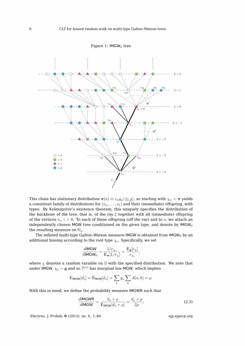
Figure 1: IMGW0 tree

qa

qc

qd

bcrsutqp

= a

= b

= c

= d

ξ

ut

ut ut ut ut

utut ut

utut

ututut

qpqpqp qp

qpqp

qp qpqpqp

qpqp qp qp

qp qp

rs

rs

rs rsrs

rs rs

rsrs rs

bc

bcbc

bcbc bc

bcbcbc bc

bc bcbcbc bc

h = −4

h = −3

h = −2

h = −1

h = 0

h = 1

h = 2

v0 = 0

v1

v2

v3

v4

v41

v42

v44

v21

v11 v12

v01

v02

v03 v04 v05

1

This chain has stationary distribution π(a) ≡ eaga/〈e, g〉, so starting with χn ∼ π yieldsa consistent family of distributions for (vn, . . . , v1) and their (immediate) offspring, withtypes. By Kolmogorov’s existence theorem, this uniquely specifies the distribution ofthe backbone of the tree, that is, of the ray ξ together with all (immediate) offspringof the vertices vi, i > 0. To each of these offspring (off the ray) and to o, we attach anindependently chosen MGW tree conditioned on the given type, and denote by IMGW0

the resulting measure on Ω↓.The inflated multi-type Galton–Watson measure IMGW is obtained from IMGW0 by an

additional biasing according to the root type χo. Specifically, we set

dIMGW

dIMGW0=

1/eχoEπ[1/eχ]

=Eg[eχ]

eχo,

where χ denotes a random variable on Q with the specified distribution. We note thatunder IMGW, χo ∼ g and so T(o) has marginal law MGW, which implies

EIMGW[do] = EMGW[do] =∑

a

ga∑

b

A(a, b) = ρ.

With this in mind, we define the probability measure IMGWR such that

dIMGWR

dIMGW=

do + ρ

EIMGW[do + ρ]=do + ρ

2ρ, (2.3)





and proceed to show that it is a reversing measure for TRWρ. From now on we adoptthe notation that if µ is a law on trees T (with or without marked ray) and a ∈ Q, µa

refers to the law conditioned on χo = a.

Proof of Thm. 1.4 (a). For the purposes of this proof we let Ω and Ω↓ be spaces of la-belled (or planar) trees (without and with marked ray, respectively), with correspondingBorel σ-algebras BΩ and BΩ↓ . We extend MGW, IMGW0, etc. to be measures on thesespaces by choosing an independent uniformly random ordering for the offspring of eachvertex. For (T, ξ) ∈ Ω↓ we use the shorthand i for vi ∈ ξ, and write (i1, . . . , idi) for itsordered offspring (with xi denoting the counts of offspring of i ≡ vi of each type).

Recalling the notation of (1.2), let S denote the map (T, ξ) 7→ (T, ξ)1. We will showthat for A,B ∈ BΩ↓ ,

∫

A

p((T, ξ), B) dIMGWR(T, ξ) =

∫

B

p((T′, ξ′), A) dIMGWR(T′, ξ′) (2.4)

where p((T, ξ), B) denotes the transition kernel of the process TRWρ. This identity im-plies reversibility of TRWρ on the space of labelled trees. Since this process projects toTRWρ on the space of unlabelled trees, the reversibility of the latter follows.

For (T, ξ) ∼ IMGW0, let IMGW←−−−a0 denote the law of the subtree T\T(i−1) rooted at i with

marked ray ξi, conditioned on the event χi−1 = a, for any i ≥ 1 (note that this lawdoes not depend on i). Then

dIMGW0(T, ξ) = π(χ1)qχ1(x1)

d1!

eχ0

〈x1, e〉dIMGW←−−−χ1

0 (T\T(1), ξ2)

d1∏

j=1

dMGWχ1j (T(1j)).

Let Pinj denote the collection of BΩ↓ -measurable sets on which S is injective, and sup-pose B ∈ Pinj. If µ is a measure on Ω↓, S∗Bµ(·) ≡ (µ S)(B ∩ ·) is a well-defined measureon Ω↓. Then

dS∗B IMGW0(T, ξ) = 1(T,ξ)∈Bπ(χ1)qχ1(x1)

d1!dIMGW←−−−

χ1

0 (T\T(1), ξ2)

d1∏

j=1

dMGWχ1j (T(1j)).

sodS∗B IMGW0

dIMGW0= 1B

ρeχ1

eχ0

.

We then verify that

dS∗B IMGW

dIMGW= 1B

( dS∗B IMGWdS∗B IMGW0

)(dIMGWdIMGW0

) dS∗B IMGW0

dIMGW0

= 1B

(dIMGWdIMGW0

S)

(dIMGWdIMGW0

) dS∗B IMGW0

dIMGW0= 1B

1/eχ1

1/eχo

ρeχ1

eχo= 1Bρ, (2.5)

and similarlydS∗B IMGWR

dIMGWR= 1B

ρ(d1 + ρ)

do + ρ.

The left-hand side of (2.4) can be written as

∫

A∩S−1B

ρ

do + ρdIMGWR(T, ξ) +

∫

A

1

do + ρ

do∑

i=1

1(T0i,ξ0i)∈B dIMGWR(T, ξ).





Using the injectivity of S on B, the second integral can be written as

∫

A∩SB

1

do + ρdIMGWR(T, ξ) =

∫

S−1A∩B

1

d1 + ρdS∗B IMGWR(T, ξ)

=

∫

S−1A∩B

ρ

do + ρdIMGWR(T, ξ).

Combining these yields an expression for the left-hand side of (2.4) which is symmetricin A and B, from which it is clear that the two sides must agree.

Since every cylinder event F can be decomposed into the disjoint union of the eventFj = (T, ξ) ∈ F : o = 1j (i.e., o is the j-th child of 1), with Fj clearly in Pinj, we havethat Pinj generates BΩ↓ . To conclude, for fixed A let B′Ω↓ denote the collection of sets

B ∈ BΩ↓ for which (2.4) holds. From the above B′Ω↓ contains the π-system Pinj. FurtherB′Ω↓ is closed under monotone limits and countable disjoint unions, and in particular it

contains Ω↓ since Ω↓ can be decomposed as a countable disjoint union of sets in Pinj bya similar argument as above. Thus by the π-λ theorem (2.4) holds for all B ∈ σ(Pinj),and extends to all B ∈ BΩ↓ again using the claim above.

The proof that IMGW is a reversing measure for the Markov pure jump processTRWcts

ρ is similar: instead of (2.4) we show that

∫

A

λ(T, ξ)p((T, ξ), B) dIMGW(T, ξ) =

∫

B

λ(T, ξ)p((T′, ξ′), A) dIMGW(T′, ξ′) (2.6)

where λ(T, ξ) ≡ λ + do is the instantaneous jump rate of the process at state (T, ξ). Asbefore, it suffices to show this for B ∈ Pinj. In this case the left-hand side of (2.6) equals

∫

A∩S−1B

ρ dIMGW(T, ξ) +

∫

S−1A∩BdS∗B IMGW(T, ξ),

which by (2.5) coincides with the right-hand side of (2.6).

2.2 Extension of IMGWR to random environment

We now extend the methods of the previous section to prove Thm. 1.7. Let e, g denote

the right and left Perron–Frobenius eigenvectors of A ≡ A(1), normalized to have sum1; as before we set g(a) ≡ MGW(χo = a) to be ga.

We proceed much as in the deterministic environment setting, although the notationbecomes more complicated. For y ∈ Q` write e(y) ≡ (eyj )

`j=1. For a ∈ Q

Eqa [〈e(y), α〉] =∑

b

A(a, b)eb = ρea,

so we define the inflated offspring measure qa by

dqa

dqa=〈e(y), α〉ρea

.

We then construct the measure IMGW0 on Ω↓ generalizing the measure IMGW0 of theprevious section: let the infinite ray ξ (without types or weights) be given, and for somen > 0 let vn have type χn. It is given offspring (yvn , αvn) ∼ qχn . One offspring w of vn isidentified with the next vertex vn−1 along ξ, where each w is chosen with probability

eχwαw〈e(y), αvn〉 .





Continuing the procedure along the ray up to v0 = o, the sequence of types χn, χn−1, . . .

seen along ξ is an irreducible Markov chain with transition probabilities

K(a, b) = Eqa

[eb∑j αj1yj=b

〈e(y), α〉

]=

ebρea

A(a, b)

and stationary distribution π(a) = eaga/〈e, g〉. Thus, starting with χn ∼ π and applyingKolmogorov’s existence theorem, we obtain a measure IMGW0 on Ω↓ which is a gener-alization of IMGW0.

Proof of Thm. 1.7. The proof is by a straightforward modification of the proof of Thm. 1.4 (a).Let S : (T, ξ) 7→ (T, ξ)1; we emphasize that S is a mapping on typed weighted labelledtrees. For (T, ξ) ∼ IMGW0, let IMGW←−−−

a0 denote the law of the subtree T\T(i−1) rooted at i

with marked ray ξi, conditioned on the event χi−1, for any i ≥ 1. Let Pinj denote thecollection of BΩ↓ -measurable sets on which S is injective. For A ∈ BΩ↓ and B ∈ Pinj, wecompute

dIMGW0(T, ξ) = π(χ1)qχ1(y1, α1)eχ0α0

〈e(y1), α1〉dIMGW←−−−χ1

0 (T\T(1), ξ2)

d1∏

j=1

dMGWχ1j

(T(1j)),

dS∗B IMGW0(T, ξ) = 1(T,ξ)∈Bπ(χ1)qχ1(y1, α1)dIMGW←−−−χ1

0 (T\T(1), ξ2)

d1∏

j=1

dMGWχ1j

(T(1j)),

so eχ0α0 dS

∗B IMGW0 = 1B ρeχ1

dIMGW0. Letting

dIMGW

dIMGW0

≡ 1/eχoEπ[1/eχ]

=Eg[χ]

eχ0

,

dIMGWR

dIMGW≡

ρ+∑doj=1 α0j

EIMGW[ρ+∑doj=1 α0j ]

=ρ+

∑doj=1 α0j

2ρ,

we obtain

α0 dS∗B IMGW = 1B ρ dIMGW,

α0

ρ+∑d1j=1 α1j

dS∗B IMGWR = 1Bρ

ρ+∑d0j=1 α0j

dIMGWR.

The analogue of (2.4) thus holds for all B ∈ Pinj, and we extend to all B ∈ BΩ↓ byessentially the same argument used in the proof of Thm. 1.4 (a).

2.3 IMGW0 as a weak limit and ergodicity

In this section we provide an alternative characterization (Propn. 2.1) of the inflatedGalton–Watson measure IMGW0, which is then used in proving the ergodicity resultThm. 1.4 (b). Propn. 2.1 is also of independent interest as a multi-type extension of [32,Lem. 1].

To this end, we will define the notion of “normalized population size” for rootedtrees T with type. Let Tn denote the subtree induced by v ∈ T : |v| ≤ n, and Dn theset v ∈ T : |v| = n. Let (Fn)n≥0 denote the natural filtration of the tree, i.e., Fn is the σ-algebra generated by Tn (a finite tree with vertex types). Let Zn = (Zn(b))b∈Q ∈ (Z≥0)Q

count the number of vertices of each type at level n, so Zn is Fn-measurable. Then

Zn ≡〈Zn, e〉ρn

=1

ρn

∑

v∈Dn

eχv





is a non-negative (Fn)-martingale under MGWa for every a, with EMGWa [Z0] = ea (seee.g. [15, p. 49]). By the normalized population size of the tree we mean the a.s. limitof Zn, denoted Wo. For v ∈ T we use Wv to denote the normalized population size ofT(v). Under (H1) and (H2), it follows from the multi-type Kesten–Stigum theorem (see[21], or the conceptual proof of [22]) that Wo > 0 a.s. on the event of non-extinction,and EMGWa [Wo] = ea.

For a ∈ Q let Qan be a probability measure on (infinite) rooted trees defined by

dQandMGWa =

Znea. (2.7)

For T ∼ Qan choose vn ∈ Dn at random with probabilities proportional to weights eχvn ,and let Qan? denote the law of the resulting pair (T, vn). Let Qn? ≡

∑a∈Q πaQ

an? and

Qn ≡∑a∈Q πaQ

an, so that dQn/dMGW = Zn/Eg[eχ]. Finally let IMGW0(n) denote the law

of (T, ξ0)vn (see (1.2) for this notation), where (T, vn) ∼ Qn? and ξ0 is any infinite rayemanating from o not sharing an edge with the geodesic from o to vn.

Proposition 2.1. Under (H1), IMGW0(n) converges weakly to IMGW0.

The proposition can be seen from the following explicit construction of Qan?: beginwith v0 ≡ o of type a, and suppose inductively that we have constructed (Ti, vi) (i < n)where Ti is the tree up to level i and vi is the i-th vertex on the geodesic from o tovn. Then vi is given offspring xvi according to qχvi , and one of these offspring w israndomly chosen (according to weights ew) to be distinguished as vi+1. Meanwhile allother vertices v ∈ Di\vi are given offspring xv according to qχv . Once (Tn, vn) hasbeen constructed, attach to each v ∈ Dn an independent MGWχv tree. For N ≥ n,

Qan?(TN , vn)

MGWa(TN )=

n−1∏

i=0

〈xvi , e〉ρeχvi

eχvi+1

〈xvi , e〉 =eχvnρnea

,

and summing over vn ∈ Dn gives (2.7).Letting n → ∞ in Qan?,Qn? we obtain the measures Qa∞?,Q∞? on rooted trees with

infinite marked ray which coincide precisely with the measures MGWa

?, MGW? of [22].

The corresponding marginals Qa∞ ≡ MGWa,Q∞ ≡ MGW on trees without marked ray

satisfydQa∞dMGWa

∣∣∣∣Fn

=Znea,

dQ∞dMGW

∣∣∣∣Fn

=Zn

Eg[eχ].

By the Kesten–Stigum theorem and Scheffé’s lemma (see e.g. [35, §5.10]), ZnL1

−→ Wo,hence

dQa∞dMGWa =

Wo

ea,

dQ∞dMGW

=Wo

EMGW[Wo]=

Wo

Eg[eχ].

We remark that although Q∞? ≡ MGW? and IMGWR are both measures on trees withrays, they are not in general equivalent unless K is reversible.

Proof of Propn. 2.1. Since dQn/dMGW = Zn/Eg[eχ] and χo ∼ g under MGW, it followsthat χo ∼ π under Qn?. It is then clear from the constructions of IMGW0 and Qn? thatif (T, ξ) ∼ IMGW0, then (T(vn), o) ∼ Qn?. In other words the portion of (T, ξ) descendedfrom vn has the same distribution under IMGW0(n) as under IMGW0, proving the result.

Turning now to the proof of Thm. 1.4 (b), it is useful to define a two-sided versionof IMGW0, as follows. Let Ωl denote the space of trees with marked line: pairs (T, ξ)

where T is an infinite tree and

ξ ≡ (. . . , ξ−1, ξ0 = o, ξ1, . . .)





is a line (doubly infinite simple path) passing through the root. The positive and nega-tive parts ξ± ≡ (ξ±j)j≥0 of ξ are edge-disjoint rays emanating from o.

Now suppose in the construction of IMGW0 we continue the backbone indefinitelyrather than stopping at o, so that Kolmogorov’s existence theorem gives a doubly infinitebackbone based on a line ξ. Attaching MGW trees to the leaves of this backbone thengives a tree with marked line (T, ξ), whose law IMGW is clearly stationary with respect tothe shift S : (T, ξ) 7→ (T, ξ)ξ−1 which defined by moving the root to ξ−1. (Alternatively, if(T, ξ) has law IMGW0 conditioned on non-extinction of T(o) and ξ is any line with ξ− = ξ,then Sn(T, ξ) converges weakly to an IMGW tree.)

It follows from the discussion preceding Propn. 2.1 that if we let

(T, ξ) ∼ IMGW0 and (T′, ξ′) ∼ Qχo∞?

(independently conditioned on χo), and we delete from T all the vertices descendedfrom o and identify o with the root of T′, then we obtain a tree with marked line ξ− = ξ,ξ+ = ξ′ whose law is precisely IMGW. It follows that the marginal law IMGW1 of (T, ξ−)

under IMGW is given bydIMGW1

dIMGW0=

dQχo∞dMGWχo

=Wo

eχo. (2.8)

Proof of Thm. 1.4 (b). We adapt the proof of [36, Cor. 2.1.25]. Abbreviating T ≡ (T, ξ),we let ν denote the law of T ≡ (Tt)t≥0 ≡ ((T, ξ)Yt)t≥0 in the space Ω∞↓ of sequences oftrees with ray, and S0 the shift (T0, T1, . . .) 7→ (T1, T2, . . .) on Ω∞↓ . The content of theresult is that the measure-preserving system (Ω∞↓ ,F

∞, ν,S0) is ergodic.

Step 1: reduction to induced system.Recall that under the measure IMGW0 the trees T(i)\T(i−1) are conditionally independentgiven the ray ξ with types, and maxa∈QMGWa(X) < 1; therefore it holds IMGW0-a.s. that|T(i)| =∞ for infinitely many i ∈ ξ. Since the walk Yt on (T, ξ) has a backward drift alongξ, this implies that if we let

A ≡T ∈ Ω∞↓ : T0 ∈ (T, ξ) ∈ Ω↓ : |T(o)| =∞

and nA(T) ≡ infn ≥ 1 : Sn0T ∈ A the first hitting time of A after time zero, then

ν(nA < ∞) = 1. Thus (Ω∞↓ , ν,S0) forms a (Kakutani) tower over the induced measure-preserving system (A, νA ≡ ν(· |A),SnA

0 ). We now show that the induced system isergodic, which is equivalent to ergodicity of the original system ([33]; see also [27, §2]).

Step 2: reduction to S-invariance.Let niA(T) denote the i-th hitting time of A after time zero and Hi ≡ σ(T0, . . . , TniA); notethat (TniA)i≥0 forms an (Hi)-Markov chain. Write S ≡ SnA

0 and let I denote the σ-fieldof S-invariant subsets of A. Fix B ∈ I, and define

φ : Ω↓ → [0, 1], φ(T) ≡ νA(T ∈ B | T0 = T).

The S-invariance of B together with the Markov property implies

νA[T ∈ B |Hi] = νA[SiT ∈ B |Hi] = νA[SiT ∈ B | TniA ] = φ(TniA),

i.e., φ(TniA) is an (Hi)-martingale. By Lévy’s upward theorem, limi→∞ φ(TniA) = 1B,νA-a.s., so that for any 0 < a ≤ b < 1,

1

t

t−1∑

i=0

1φ(TniA

)∈[a,b]





converges νA-a.s. to zero. On the other hand, by the Birkhoff ergodic theorem (see e.g.[11, Thm. 6.2.1]), it converges νA-a.s. to νA(φ(T) ∈ [a, b] | I). Taking expectations onboth sides we find φ(T) ∈ 0, 1 νA-a.s., that is, φ = 1C0

for some C0 ∈ BΩ↓ . Further,since φ is a 0, 1-valued martingale, it holds ν-a.s. that T0 ∈ C0 if and only if TnA ∈ C0.Since νA(TnA = ST0) > 0 where S is as defined above, 1C0

≤ 1S−1C0νA-a.s. Applying

the same argument with the martingale 1− φ gives 1C0= 1S−1C0

νA-a.s., i.e., that C0 isS-invariant.

Step 3: IMGWR-triviality of S-invariant sets.It follows from B ⊆ A that C0 is a subset of A0 ≡ (T, ξ) ∈ Ω↓ : |T(o)| = ∞. SinceIMGWR IMGW1 on A0 by (2.8), the result follows by showing that S-invariant subsetsof A0 are IMGW1-trivial. For any C ′0 ⊆ A0 let C ′0 ≡ (T, ξ) : (T, ξ−) ∈ C ′0; the S-invariance of C0 implies S-invariance of C0. But the ergodicity of the Markov chain oftypes along the line ξ readily implies that S-invariant subsets of A0 are IMGW-trivial, e.g.by the following modification of the argument of [18, Thm. 2.15]: take Cn0 measurablewith respect to the portion ξ[−n,0] of the line between ξ−n and o, together with thedescendant subtrees of ξ−n, . . . , ξ−1 away from ξ, such that the symmetric differenceCn04C0 has IMGW-measure tending to zero in n. It follows from S-invariance of C0

together with S-stationarity of IMGW that IMGW[Cn04C0] = IMGW[(SmCn0 )4C0] for anym, so (by the triangle inequality)

limn→∞

supm|IMGW(C0)− IMGW[Cn0 ∩ (SmCn0 )]| = 0.

But for any m > n we have

IMGW[Cn0 ∩ (SmCn0 )] = IMGW[ξ[−n,0], ξ[m−n,m]]IMGW[Cn0 | ξ[−n,0]]IMGW[SmCn0 | ξ[m−n,m]],

which tends as m→∞ to IMGW[Cn0 ]2. Therefore

IMGW[C0] = limn→∞

IMGW[Cn0 ] = limn→∞

IMGW[Cn0 ]2 = IMGW[C0]2

which gives IMGW[C0] ∈ 0, 1 as required.

3 Harmonic coordinates and quenched IMGWR-CLT

In this section we prove the quenched IMGWR-CLT Thm. 1.5. Let

η ≡ EQ∞ [Wo] =EMGW[W 2

o ]

Eg[eχ], σ2 ≡ Eg[eχ]2

EMGW[W 2o ]. (3.1)

In §3.1 we construct harmonic coordinates for RWρ on IMGWR-a.e. (T, ξ), and use theergodicity result Thm. 1.4 (b) proved above to show an IMGWR-a.s. CLT for the martin-gale Mt ≡ SYt , with Mbntc/(ησ

√n) converging to standard Brownian motion. In §3.2

we control the error between h(Yt) and Mt/η to prove Thm. 1.5. The following result,whose proof is deferred to §6.2, implies finiteness of η and σ under (H32):

Proposition 3.1. If (H1), (H2), and (H3p) hold with p > 1, then EMGW[W po ] <∞.

3.1 Harmonic coordinates for RWρ and martingale CLT

From now on, if µ is a probability measure on trees (with or without marked ray),we use µ as shorthand also for µ ⊗ RWρ. We write PT for the law of the quenchedrandom walk RWρ(T) and ET for expectation with respect to PT, and let (GT

t )t≥0 denotethe corresponding filtration of the walk. Given T, for a vertex v ∈ T we let ∂v denotethe neighbors of v, and ∂+v the offspring of v, i.e., ∂+v = ∂v ∩ T(v). We write v ≤ w ifw ∈ T(v), with v < w if w 6= v.





For v ∈ T recall that Wv denotes the normalized population size of the subtree T(v).2

For vertices v ∈ T we define Sv as in [32, §3]: if T is a rooted tree, let

Sv ≡∑

o<u≤v

Wu. (3.2)

If T has marked ray ξ, recalling (1.1) we set

Sv ≡ SRv + Sξv where SRv ≡ −∑

u∈ξ,o≥u>Rv

Wu, Sξv ≡∑

Rv<u≤v

Wu. (3.3)

While on MGW-a.e. T the map v 7→ Sv is harmonic except at o with respect to thetransition probabilities of RWρ(T), on IMGW-a.e. (T, ξ) the map v 7→ Sv is harmonic atevery vertex with respect to the transition probabilities of RWρ(T, ξ). Thus, if (Yt)t≥0 ∼RWρ(T, ξ), Mt ≡ SYt will be a martingale given a fixed realization of the tree; we re-gard it as providing “harmonic coordinates” for the random walk. Using the reversingmeasure IMGWR it is easy to prove a quenched CLT for M (extending [32, Cor. 1]):

Proposition 3.2. Under (H1), (H2), and (H32), on IMGW-a.e. (T, ξ) the processMbntc/(ησ√n)

converges in distribution to a standard Brownian motion as n→∞.

Proof. We check the conditions of the Lindeberg–Feller martingale CLT (see e.g. [11,Thm. 7.7.4]): letting

Vn =1

n

n−1∑

t=0

ET[(Mt+1 −Mt)2 |GT

t ],

we verify that for IMGW-a.e. (T, ξ),

(i) Vn → η2σ2 in probability and

(ii) for all ε > 0, 1n

∑n−1t=0 ET[(Mt+1 −Mt)

21|Mt+1−Mt|>ε√n]→ 0.

Let Yn denote the random walk on (T, ξ): we rewrite Vn in terms of the induced randomwalk on Ω↓ as

Vn =1

n

n−1∑

t=1

ϕ[(T, ξ)Yt ], ϕ[(T, ξ)] ≡ ρ

ρ+ doW 2o +

1

ρ+ do

do∑

j=1

W 20j .

By Thm. 1.4 (b) and the Birkhoff ergodic theorem, we have Vn converging IMGWR-a.s.to EIMGWR[ϕ] provided ϕ ∈ L1(IMGWR). We calculate

EIMGWR[ϕ] =1

2ρEMGW

[ρW 2

o +∑

v∈∂o

W 2v

]= EMGW[W 2

o ] = η2σ2,

so condition (i) is proved. Condition (ii) is checked similarly using dominated conver-gence.

Remark 3.3. To give some indication of how our results might be extended to RWREρ,we note that the main ingredient needed is the appropriate generalization of the nor-malized population size: we define it to be the random variableW o which is the a.s. limitof the martingale Zn ≡ Z

(1)n defined by (5.1). If W v denotes the normalized population

size of T(v), thenρW v =

∑

w∈∂+v

αwWw,

2Note that if T has a marked ray ξ, then for v ∈ ξ, Zvn = 〈Zvn, e〉/ρn is not necessarily a martingale for thefirst |h(v)| steps. Nevertheless it is eventually a martingale so we can still define Wv to be the a.s. limit ofZvn.





so the W v can be used to define harmonic coordinates for the RWRE. In the single-type case, W o has finite second moment if and only if κ ≥ 2 [24, Thm. 2.1], so clearlyPropn. 3.2 cannot apply outside this regime. We emphasize again that due to the sametechnical barriers which arise in [13], simple adaptations of our proof will not cover thefull regime κ ≥ 2.

3.2 Quenched IMGWR-CLT

We now prove the quenched CLT for IMGWR trees by controlling the corrector

εt ≡Mt

η− h(Yt)

on the interval 0 ≤ t ≤ n. For 1/2 < δ < 1 and n ≥ 0 fixed, let τn(j), for jbnδc ≤ n

denote integer times chosen uniformly at random (independently of one another and ofthe random walk Y ) from the interval [jbnδc, (j + 1)bnδc).Proposition 3.4. Assume (H1), (H2), and (H3p) with p > 2. There exists δ0 ≡ δ0(p) ∈(1/2, 1) such that for δ0 ≤ δ < 1 and ε > 0,

limn→∞

P(T,ξ)

(max

jbnδc≤n

∣∣ετn(j)

∣∣ ≥ ε√n)

= 0, IMGWR-a.s. (3.4)

Further, for any ε′ with 2ε′ + δ < 1,

limn→∞

P(T,ξ)

(max

r,s≤n,|r−s|≤nδ|h(Yr)− h(Ys)| ≥ n1/2−ε′

)= 0, IMGWR-a.s. (3.5)

Given this proposition, we can prove the quenched CLT for RWρ on IMGWR trees:

Proof of Thm. 1.5. If t ≤ n then |t− τn(j)| ≤ bnδc for some j, so

maxt≤n|εt| ≤ max

r,s≤n,|r−s|≤bnδc

∣∣∣∣Mr

η− Ms

η

∣∣∣∣+ maxjbnδc≤n

|ετn(j)|+ maxr,s≤n,|r−s|≤bnδc

|h(Yr)− h(Ys)|.

M satisfies a CLT by Propn. 3.2, and it follows from (3.4) and (3.5) that

limn→∞

P(T,ξ)

(maxt≤n|εt| ≥ ε

√n)

= 0, IMGWR-a.s.,

which gives the result.

The remainder of this section is devoted to the proof of Propn. 3.4.

3.2.1 Tightness

We begin by proving (3.5), using some a priori (annealed) estimates for RWρ comingfrom the Carne–Varopoulos bound.

Lemma 3.5. There exists a constant C <∞ such that

MGW(

maxt≤n|Xt| ≥ m

)≤ Cne−(m+1)2/(2n) ∀m,n ≥ 1.

Proof. We modify the proof of [32, Lem. 5]. Take the finite tree with vertices w ∈ T :

|w| ≤ m, and make this into a wired tree T? by adding a new vertex o? which is joinedby an edge to each vertex in Dm. Define the modified random walk X? on T? whichfollows the law of RWρ except at o? where it moves to a vertex chosen uniformly atrandom from Dm. Then

PT(maxt≤n|Xt| ≥ m) ≤ 2

n+1∑

t=1

PT?(Xt = o?).





By the Carne–Varopoulos inequality (see [29, Thm. 13.4]),

PT?(X?t = o?) ≤ 2

√|Dm|ρm−1

e−(m+1)2/(2t).

Taking expectations gives

MGW(|X?t | = o?) ≤ Ce−(m+1)2/(2t),

and summing over 1 ≤ t ≤ n+ 1 gives the result.

Corollary 3.6. There exists a constant C <∞ such that for any m,n ≥ 1,

C−1 IMGW0

(maxt≤n|h(Yt)| ≥ m

)≤ IMGWR

(maxt≤n|h(Yt)| ≥ m

)≤ Cn2e−m

2/(2n).

Proof. We argue as in the proof of [32, Cor. 2]. By decomposing into at most n excur-sions away from height zero and using the stationarity of IMGWR, we find

IMGWR(

maxt≤n

h(Yt) ≥ m)

≤ n IMGWR(∃t ≤ n : h(Yt) ≥ m,h(Ys) > 0 ∀0 ≤ s ≤ t

)

≤ CnMGW(

maxt≤n|Xt| ≥ m− 1

)≤ Cn2e−m

2/(2n),

by Lem. 3.5. The same bound holds for IMGWR(mint≤n h(Yt) ≤ −m) by the reversibilityof IMGWR. The result follows by noting that dIMGW0/dIMGWR is uniformly bounded bya deterministic constant.

Proof of Propn. 3.4, (3.5). By stationarity of IMGWR and Cor. 3.6, for any fixed s

IMGWR(

max0≤u≤nδ

|h(Ys+u)− h(Ys)| ≥ n1/2−ε′)≤ Cn2δe−n

1−2ε′−δ/2,

and summing over s ≤ n gives

IMGWR(

maxr,s≤t,|r−s|≤nδ

|h(Yr)− h(Ys)| ≥ n1/2−ε′)≤ Cn2δ+1e−n

1−2ε′−δ/2,

which is summable in n provided 2ε′ + δ < 1. The result then follows from Markov’sinequality and Borel–Cantelli.

3.2.2 Control of corrector

In the remainder of this section we prove (3.4). We will make use of the followingclassical result:

Lemma 3.7 ([34, p. 60]). If z1, . . . , zn are independent random variables with Ezi = 0

and E|zi|p <∞, then

E

[∣∣∣∣n∑

i=1

zi

∣∣∣∣p]≤

2∑ni=1E[|zi|p] if 1 ≤ p ≤ 2,

C(p)np/2−1∑ni=1E[|zi|p] if p ≥ 2.

Recalling (1.1) and (3.3), we decompose

1√n

maxjbnδc≤n

∣∣ετn(j)

∣∣ ≤ E1 + E2 (3.6)





where, with Rt ≡ RYt denoting the nearest ancestor of Yt on ξ,

E1 ≡1√n

maxt≤2n

∣∣∣∣SRtη− h(Rt)

∣∣∣∣ , E2 ≡1√n

maxjbnδc≤n

∣∣∣∣∣SξYτn(j)

η− d(Yτn(j), ξ)

∣∣∣∣∣ .

The following lemma says that the harmonic coordinates (Sv)v∈T of (3.2), rescaled byη of (3.1), are a good approximation to the actual coordinates |v| on the MGW rootedtrees. Let

Aεn ≡ Aεn(T) ≡v ∈ Dn :

∣∣∣∣Svn− η∣∣∣∣ > ε

, ε > 0, n ≥ 1. (3.7)

Let τ ≡ mint > 0 : Xt = o denote the first return time to the starting point X0 = o

by the walk X.

Lemma 3.8. Assume (H1), (H2), and (H3p) with p ≥ 2. For any ε > 0, the expectednumber of visits to Aεk during a single excursion away from the root is

EMGW

[ τ∑

t=0

1Xt∈Aεk

]≤ C

ρkEMGW

[ ∑

v∈Aεk

(1 + dv)

]≤ C(p, ε)

kp/2.

Proof. If v ∈ T with |v| = k ≥ 1, a simple conductance calculation (see [29, Ch. 2]) gives

ET

[ τ∑

t=0

1Xt=v

]=PT(o→ v)

PT(v → o)=ρ+ dvdoρk

, (3.8)

so the first inequality follows. For the second we follow the proof of [32, Lem. 3] (inparticular the estimate [32, (20)]) and of [13, Lem. 4.2]. Recall from §2.3 the definition(2.7) of the probability measure Qak on rooted trees T given by a size-biasing of MGWa,and further the probability Qak? on rooted trees T with a marked path (o = v0, . . . , vk)

from the root to level k:

EMGWa

[ ∑

v∈Aεk

(1 + dv)

]≤ CEMGWa

[ ∑

v∈Aεk

eχv (1 + dv)

]

≤ CρkEQa

[∑v∈Aεk

eχv (1 + dv)

〈Zk, e〉

]= CρkEQak?

[(1 + dvk)1vk∈Aεk],

so it suffices to show

EQak?[(1 + dvk)1vk∈Aεk] ≤ C(p, ε)k−p/2.

To this end, writing Wi ≡ Wvi , for i < k we decompose Wi ≡ Wi+1/ρ+W 8i where W 8i isthe normalized population size of T(vi)\T(vi+1). Then

Wi =

k−1∑

j=i

W 8jρj−i

+Wk

ρk−i,

soSvkk− η =

1

kCkWk +

1

k

k−1∑

i=1

CiW8i − η, Ci ≡

i−1∑

j=0

ρ−j ≤ C∞ ≡ρ

ρ− 1.

Conditional on the types (χi ≡ χvi)ki=1, the random variables W 81, . . . ,W8k−1 are indepen-

dent of one another and of the pair (Wk, dvk), and all these random variables have finitemoments of order p by Propn. 3.1. Therefore

EQak?[(1 + dvk)1vk∈Aεk] ≤ CQ

ak?

(∣∣∣∣1

k

k−1∑

i=1

CiW8i − η

∣∣∣∣ ≥ ε/2)

+ EQak?[(1 + dvk)1CkWk/k≥ε/2]





By (H3p), Markov’s inequality, and Hölder’s inequality, the second term is

≤(

2Ckkε

)p−1

EQak?[(1 + dvk)W p−1

k ] ≤ C(p, ε)

kp−1≤ C(p, ε)

kp/2

(since p ≥ 2). As for the first term, by Lem. 3.7 and Markov’s inequality,

Qak?

(∣∣∣∣1

k

k−1∑

i=1

CiW8i − EQak?

[1

k

k−1∑

i=1

CiW8i

∣∣∣∣ (χi)ki=1

]∣∣∣∣ > ε/4

)

≤ C(p)kp/2−1

(kε)p

k−1∑

i=1

EQak?[|Ci(W 8i − E[W 8i |χi])|p]

≤ C(p, ε)k−p/2.

On the other hand,

EQak?

[1

k

k−1∑

i=1

CiW8i

]→ C∞EQ∞ [W 8o] = EQ∞ [Wo] = η,

and so

Qak?

(∣∣∣∣EQak?

[1

k

k−1∑

i=1

CiW8i

∣∣∣∣ (χi)ki=1

]− η∣∣∣∣ > ε/4

)

decays exponentially in k by [10, Thm. 3.1.2]. Combining these estimates completes theproof.

Recalling the definition (3.3) of the harmonic coordinates on the IMGWR trees, thenext step is to use Lem. 3.8 to show that on these trees Sξv/η is a good approximation tod(v, ξ). In analogy with (3.7) set

Bεk =

w ∈ T : d(w, ξ) = k,

∣∣∣∣Sξwk− η∣∣∣∣ > ε

, Bε =

⋃

k≥1

Bεk(T, ξ). (3.9)

Lemma 3.9. Assume (H1), (H2), and (H3p) with p > 2. There exists δ0 ≡ δ0(p) ∈ (1/2, 1)

such that for δ0 ≤ δ < 1 and ε > 0,

limn→∞

P(T,ξ)

(∃j ∈ Z≥0, jbnδc ≤ n : Yτn(j) ∈ Bε

)= 0, IMGWR-a.s.

Proof. We modify the proof of [13, (22)]. If we define

τhitn,ε ≡ inft ≥ 0 : |h(Yt)| = bn1/2+εc,

then Cor. 3.6 together with Markov’s inequality gives

IMGWR[P(T,ξ)(τhitn,ε ≤ n) ≥ c] ≤ c−1IMGWR(τhit

n,ε ≤ n) ≤ c−1Cn2e−n2ε/2,

so by Borel–Cantelli we have P(T,ξ)(τhitn,ε ≤ n)→ 0, IMGWR-a.s.

On the event τhitn,ε > n, we decompose the walk into excursions from ξ started at

vi, 0 ≤ i < bn1/2+εc (with each step of the walk along the ray contributing an emptyexcursion) and apply Wald’s identity (see e.g. [4, Exercise 22.8]) to find

P(T,ξ)

(∃jbnδc ≤ n : Yτn(j) ∈ Bε

∩ τhit

n,ε > n)

≤ 1

bnδc

bn1/2+εc−1∑

i=0

E(T,ξ)[Li(τhitn,ε)]E

i(T,ξ)[L(Bε; τ exc)]. (3.10)





In the above, LA(n) ≡ L(A;n) denotes the number of visits to set A by time n andLi(n) ≡ L(vi;n). Ei(T,ξ) denotes expectation with respect to the law of a ρ-biased random

walk Y started from Y0 = vi, and τ exc ≡ inft > 0 : Yt = vi or Yt /∈ T(vi) denotes theexcursion end time.

By a conductance calculation,

E(T,ξ)[Li(τhitn,ε)] =

1

P(vi → vbn1+εc)≤ 1 + di/ρ

1− ρ ≤ Cdi. (3.11)

During a single excursion away from ξ the walk can visit only one of the T(w) for w ∈∂+v\vi−1, so to bound the second factor of each summand in (3.10) it suffices to consideran MGW rooted tree T′ (without ray): letting

Aεk ≡ Aεk(T′) ≡v ∈ Dk :

∣∣∣∣Wo + Svk + 1

− η∣∣∣∣ > ε

, Aε ≡

⋃

k≥0

Aεk,

it follows from a (very slight) modification of Lem. 3.8 that

EIMGW0[L(Bε; τ exc) | i ∪ ∂+i] ≤ CEMGW

[ τ∑

t=0

1Xt∈Aε

]≤ C(p, ε)

∑

k≥1

k−p/2 ≤ C(p, ε)

(using p > 2). It follows that the quantity in (3.10) converges to zero IMGWR-a.s., whichconcludes the proof.

Proof of Propn. 3.4, (3.4). Recall the decomposition (3.6). For any k0,

E1 ≤1√n

maxi≤k0

∣∣∣∣Sviη− h(vi)

∣∣∣∣+1√n

maxt≤2n,h(Rt)>k0

∣∣∣∣SRtη− h(Rt)

∣∣∣∣ .

The first term clearly tends to zero as n→∞ with k0 fixed. The second term is boundedabove by (

1√n

maxt≤2n

|Mt|)

supi>k0

∣∣∣∣1

η− h(vi)

Svi

∣∣∣∣ . (3.12)

Now recall from the proof of Propn. 2.1 that if (T, ξ) ∼ IMGW0 then (T(k), o) ∼ Qk?. Thusa consequence of the proof of Lem. 3.8 is that for sufficiently small ε,

IMGW0(|Svk/k + η| ≥ ε) ≤ C(p, ε)k−p/2.

Therefore the supremum in (3.12) can be made arbitrarily small by taking k0 large. Wealso have

E2 ≤(

1√n

maxt≤2n

|Mt|)

maxjbnδc≤n

∣∣∣∣∣1

η− d(Yτn(j), ξ)

SξYτn(j)

∣∣∣∣∣ ,

and in view of Lem. 3.9 the second factor tends to zero in probability. By the invarianceprinciple for M proved in Propn. 3.2, maxt≤2n |Mt|/

√n stays bounded in probability as

n→∞, so the result follows.

4 From IMGWR-CLT to MGW-CLT by shifted coupling

In this section we prove our main result Thm. 1.1. In §4.1 we review (a slight modifi-cation of) the “shifted coupling” procedure of [32, §6], which we use in §4.2 to transferthe IMGWR-CLT to an annealed MGW-CLT. In §4.3 we prove a variance estimate whichallows to go from the annealed to the quenched MGW-CLT.





4.1 The shifted coupling construction

We begin by reviewing the shifted coupling construction of [32, §6], with the mod-ification needed to handle the multi-type case. The basic observation underlying theconstruction is that the law of the random walk X ∼ RWρ(T) up to time t depends onlyon

Et ≡ o ∪ (∂Xs)0≤s<t

(“the subtree explored by time t”), so that one can construct the tree at the same timeas the random walk.

For any tree T (with or without marked ray) and U any subset of the vertices of T,we also use U to indicated the subgraph of T induced by U . Let LT denote the set ofleaves of T, and write T ≡ T\LT.

Let a0 ∈ Q be fixed, and suppose (T, (Xt)t≥0) ∼ MGW ⊗ RWρ. For each fixed n ≥ 1

we give a decomposition of X into “fresh excursions” marked by time intervals [τi, ηi),i ≥ 1 (all depending on n), as follows. Set η0 ≡ 0 and define

`(n) ≡ 4b(log(1 + n))3/2c. (4.1)

For i ≥ 1, let

τi ≡ mint > ηi−1 : Xt ∈ LEt, |Xt| > `(n)/2, χXt = a0, excursion start,

ηi ≡ mint > τi : Xt ∈ Eτi, excursion end,

Vi ≡ Xτi ∪ Eηi\Eτi , excursion exploration.

We take the convention min∅ ≡ ∞, and let τX ≡ max i : ηi <∞ be the total numberof excursions (so

τX <∞

= X). The key point of the above definition is that even

after X reaches a leaf vertex and it is necessary to grow the tree to continue samplingthe random walk, we do not consider a fresh excursion (Xs)τi≤s<ηi to have begun untilX reaches a leaf vertex of the fixed type a0. Without this restriction the sequence oftypes (χXτi )i≥1 has a possibly complicated dependency structure making it unclear howto define a valid coupling.

Next we construct a coupled realization ((T, ξ), (Yt)t≥0) ∼ IMGW0 ⊗ RWρ as follows:first construct the backbone E0 of the tree (ξ and ∂+vi for i ≥ 1, together with types)in the manner described in §2.1. Set η0 ≡ 0, and start a ρ-biased random walk Y on E0with Y0 = o. As in the MGW setting we will construct a growing sequence (Et )t≥0 suchthat Et = E0 ∪ (∂Ys)0≤s<t, and we will define (for i ≥ 1)

τi ≡ mint > ηi−1 : Yt ∈ LEt , d(Yt, ξ) > `(n)/2, χYt = a0, excursion start,

ηi ≡ mint > τi : Yt ∈ (Eτi ), excursion end,

Vi ≡ Yτi ∪ Eηi \Eτi, excursion exploration.

The difference is that we grow the sequence Et in a manner dependent on (T, X),such that excursions of Y into unexplored territory (and started from a0) match theexcursions of X defined above: formally, we couple (Ys)τi ≤s<ηi with (Xs)τi≤s<ηi suchthat there is a (type-preserving) isomorphism fi : Vi → Vi with fi(Xτi+s) = Yτi +s, andthen we set Yηi to be the ancestor of Yτi (not necessarily of the same type as Xηi).Then, on the inter-excursion intervals ηi−1 ≤ t < τi (for i ≥ 1),

• If Yt ∈ (Et ) then generate Yt+1 according to the transition kernel of RWρ on

Et+1 = Et ;

• If Yt ∈ LEt with χYt 6= a0, let Et+1 be the enlargement of Et obtained by attachingrandom offspring to Yt according to law qχYt , and generate Yt+1 according to thetransition kernel of RWρ on Et+1.





Again, a fresh excursion (Ys)τi ≤s<ηi does not begin until Y reaches a leaf vertex of thecorrect type a0. Finally, with E∞ ≡ limt→∞ Et , we define T by attaching to each vertexv ∈ LE∞ an independent MGWχv tree. We thus obtain the following extension of [32,Lem. 8]:

Lemma 4.1. If (T, (Xt)t≥0) ∼ MGW ⊗ RWρ then the marginal law of ((T, ξ), (Yt)t≥0)

arising from the above construction is IMGW0 ⊗ RWρ.

Remark 4.2. Although we suppress the parameter n from the notation, we emphasizethat each n ≥ 1 gives rise to a different excursion decomposition, hence a differentcoupling between (T, X) and ((T, ξ), Y ).

4.2 Annealed MGW-CLT

We now transfer the quenched IMGWR-CLT to the following annealed MGW-CLT:

Proposition 4.3. Assume (H1), (H2) and (H3p) with p > 4. If (T, X) has law MGW ⊗RWρ conditioned on Xc, then the processes (|Xbntc|/(σ

√n))t≥0 converge in law to the

absolute value of a standard Brownian motion.

Recall that Rt ≡ RYt denotes the nearest ancestor of Yt on ξ. By Thm. 1.5, forIMGW0-a.e. (T, ξ), the process

Hbntc/(σ√n), Ht ≡ h(Yt)− min

0≤s≤th(Ys) = h(Yt)− min

0≤s≤th(Rs) ≥ 0 (4.2)

converges to a Brownian motion minus its running minimum, which is the same in lawas the absolute value of a Brownian motion (see e.g. [19, Thm. 3.6.17]). Thus to deducePropn. 4.3 we need to estimate the relation between the processes |Xn| and Hn. To thisend, let t, t be the monotone increasing bijections

t : Z≥0 →⋃

i≥1

[ηi−1, τi), t : Z≥0 →⋃

i≥1

[ηi−1, τi ),

parametrizing the inter-excursion times of Xn and Yn respectively. We make the follow-ing notations (the left column refers to the MGW tree, while the right column refers tothe IMGW0 tree):

X ints ≡ Xt(s), Y int

s ≡ Yt(s)Hs ≡ σ(Xt : t ≤ t(s)) Hs ≡ σ(Yt : t ≤ t(s)),

Ji ≡ t−1[ηi−1, τi), Ji ≡ (t)−1[ηi−1, τi );

In ≡ max i : ηi−1 ≤ n , In ≡ maxi : ηi−1 ≤ n

;

∆n ≡∑Ini=1 |Ji|, ∆n ≡

∑Ini=1 |Ji |;

∆n(α) ≡∑Ini=1 |s ∈ Ji : |X int

s | ≤ nα|, ∆n(α) ≡∑Ini=1 |s ∈ Ji : d(Y int

s , ξ) ≤ nα|.

In words, given the walk X on the MGW tree, X ints is the “inter-excursion process”

adapted to the filtration Hs, Ji is the i-th inter-excursion interval, In is the number ofsuch intervals intersecting [0, n], ∆n is the total length of these intervals, and ∆n(α) isthe length of these intervals except for times spent at distance more than nα from theroot. The right column defines the analogous objects for the walk on the IMGW0 tree.

Lemma 4.4. Assume (H1), (H2), and (H3p) with p > 4. There exists α0(p) < 1/2 suchthat for α > α0(p),

MGW(∆n(α) 6= ∆n |Xc)

IMGW0(∆n(α) 6= ∆n)

≤ n−c, c ≡ c(p, α) > 0.

We will obtain the corollary below as a relatively straightforward consequence ofLem. 4.4. Let

Dn ≡ max0≤r≤s≤n

h(Rs)− h(Rr)





denote the maximum displacement by time n against the backward drift on ξ.

Corollary 4.5. Assume (H1), (H2), and (H3p) with p > 4. Then

(a) There exists α0(p) < 1/2 such that for α ≥ α0(p),

MGW(∆n ≥ n1/2+α+ε |Xc)

IMGW0(∆n ≤ n1/2+α+ε)

≤ n−c, c ≡ c(p, α, ε) > 0

(b) On IMGW0-a.e. (T, ξ), Dn/√n converges P(T,ξ)-a.s. to zero.

Assuming these results we can prove the annealed MGW-CLT:

Proof of Propn. 4.3. Let b : Z≥0 → Z≥0 be any nondecreasing map which maps [τi , ηi )

bijectively onto [τi, ηi), and Ji into Ji, for each i. Then for t ∈ [τi , ηi ) we have |Xb(t)| −

|Xτi | = d(Yt, ξ)− d(Yτi , ξ), so, recalling (1.1) and (4.2), we have

||Xb(t)| −Ht| =∣∣∣∣|Xb(t)| − d(Yt, ξ)− h(Rt) + min

s≤th(Rs)

∣∣∣∣ ≤ |Xτi |+ d(Yτi , ξ) +Dt.

If instead t ∈ Ji then

||Xb(t)| −Ht| ≤ |Xb(t)|+ |Ht| ≤ |Xb(t)|+Dt + d(Yt, ξ).

It follows that on the event ∆n(α) = ∆n ∩ ∆n(α) = ∆n,

1√n

max0≤t≤n

||Xb(t)| −Ht| ≤2nα +Dn√

n,

so by Thm. 1.5, Lem. 4.1, Lem. 4.4, and Cor. 4.5 (b), the processes (|Xb(bntc)|/(σ√n))t≥0

converge in law to a reflected Brownian motion. On the other hand, Cor. 4.5 (a) im-plies that n−1 max0≤t≤1(b(bntc)− bntc)→ 0 in probability, so we obtain the CLT for theprocesses (|Xbntc|/(σ

√n))t≥0 from the a.s. uniform continuity of Brownian motion on

compact intervals.

In the remainder of this subsection we prove Lem. 4.4 and Cor. 4.5. Let Co,` ≡C(o↔ `) denote the conductance between o and D` in T, with respect to the stationarymeasure $ for RWρ(T) with the normalization $(o) = do. We will make use of thefollowing conductance lower bound:

Lemma 4.6. Under (H1), (H2), and (H32), there exist 0 < r,C < ∞ such that for allε > 0, MGW(C−1

o,k ≥ k1+ε |Xc) ≤ Ck−rε.The proof of the lemma is deferred to §6.3 where we also provide a quenched con-

ductance lower bound (see Propn. 6.5) which is not needed in the proof of the maintheorem. Lem. 4.6 readily implies an upper bound on the amount of time

Nα(n) ≡n∑

t=0

1|Xt|≤nα, Nα(n) ≡n∑

t=0

1d(Yt,ξ)≤nα

spent by X (resp. Y ) within distance nα of the root (resp. marked ray) by time n:

Corollary 4.7. Assume (H1), (H2), and (H32). Then

MGW(Nα(n) ≥ n1/2+α+ε |Xc)

IMGW0(Nα(n) ≥ n1/2+α+ε)

≤ Cn−cε.





Proof. By iterated expectations, Markov’s inequality, and Lem. 3.5,

MGW(Nα(n) ≥ n1/2+α+2ε |Xc) ≤ n−ε + MGW(ET[Nα(n)] ≥ n1/2+α+ε |Xc)

≤ n−ε + Ce−n2ε/3 + MGW(τhit

n,ε > n ∩ ET[Nα(τhitn,ε)] ≥ n1/2+α+ε |Xc)

where τhitn,ε ≡ inft ≥ 0 : |Xt| = bn1/2+εc. Wald’s identity gives

ET[Nα(τhitn,ε)] ≤ ET[Lo(τ

hitn,ε)]ET[Nα(τ)]

with LA(n) the number of visits the walk makes to set A by time n. Recalling (3.8), wehave

ET[Lo(τ)] ≤ doC(o↔ bn1/2+εc) , ET[Nτ(α)] ≤ C

bnαc+1∑

k=0

|Dk|,

so the MGW bound follows from Lem. 4.6 with a few more applications of Markov’sinequality.

For the IMGW0 bound we argue as in the proof of Lem. 3.9: by Markov’s inequalityand Cor. 3.6,

IMGW0(Nα(n) ≥ n1/2+α+2ε) ≤ n−ε + IMGW0(E(T,ξ)[Nα(n)] ≥ n1/2+α+ε)

≤ n−ε + Ce−n4ε/3 + IMGW0(Nα(τhit

n,ε) ≥ n1/2+α+2ε),

so it suffices to bound the last term. By Wald’s identity and (3.11),

E(T,ξ)[Nα(τhit

n,ε)] ≤bn1/2+εc−1∑

i=0

E(T,ξ)[Li(τhitn,ε)]E

i(T,ξ)[N

α(τ exc)]

≤ Cbn1/2+εc−1∑

i=0

diEi(T,ξ)[N

α(τ exc)],

so again the bound follows by using Markov’s inequality.

Most of the technical estimates required for the proof of Lem. 4.4 are containedin the following auxiliary lemma (cf. [13, Lem. 7.3]). For `(n) as in (4.1), define thesequence of (Hs)-stopping times

Θ0 ≡ 0, Θj+1 ≡ mins > Θj : ||X ints | − |X int

Θj | = `(n)|

and similarly the sequence of (Hs)-stopping times

Θ0 ≡ 0, Θj+1 ≡ mins > Θj : |d(Y ints , ξ)− d(Y int

Θj, ξ)| = `(n).

Lemma 4.8. Assume (H1) and (H2).

(a) Assume (H3p) and let

C ≡ C(n, ε) ≡ v ∈ T : Wv > n1/4−ε

(well-defined for trees with and without ray). Then

MGW(τhit(C) ≤ n)

IMGW0(τhit(C\ξ) ≤ n)

≤ C(p, ε)n1−p(1/4−ε).

For p > 4 the right-hand side can be made ≤ n−c for c ≡ c(p, ε) > 0.





(b) Assuming (H3p) with p > 2, for any ε > 0 there exists c ≡ c(p, ε) such that

MGW(In ≥ n1/2+ε |Xc)

IMGW0(In ≥ n1/2+ε)

≤ e−cnε/2 .

(c) With Θj ,Θj defined as above,

MGW(t(Θ3In) ≤ n)

IMGW0(t(Θ3In) ≤ n)

≤ e−c`(n).

(d) Recalling the notation of (3.7) and (3.9), define

A ≡ A(n, α, ε) ≡b(logn)2c⋃

k=0

Aεbnαc−k, B ≡ B(n, α, ε) ≡b(logn)2c⋃

k=0

Bεbnαc−k.

Assuming (H3p) with p > 2, there exists α0(p) ∈ (0, 1/2) such that for all α ≥ α0(p)

and all ε < ε0(p, α) (with ε0(p, α) > 0),

MGW(τhitA ≤ n)

IMGW0(τhitB ≤ n)

≤ n−c (4.3)

for some c ≡ c(p, α, ε) > 0. If further p > 4 then α0, ε0 can be chosen such that

MGW(τhitA+≤ n) ≤ n−c, A+ ≡ A+(n, α, ε) ≡

⋃

k≥bnαc

Aεk. (4.4)

Proof. (a) See proof of [32, (63)].

(b) We will show that with probability ≥ 1 − e−cnε/2

conditioned on Xc, one of thefirst bn1/2+ε/2c excursions has length ηi − τi > n which certainly implies the result.Conditioning on Xc is needed simply to ensure τX = ∞; for the purpose of proving theclaim we may artificially define ηi − τi =∞ for i > τX.

Then, conditioned on (ηj − τj)i−1j=1, the probability that ηi − τi > n is bounded below

by a constant times MGW(τ > n). Further

PT(τ > n) ≥ PT(τ > τhitn,ε/2 > n) ≥ PT(τ > τhit

n,ε/2)− PT(τhitn,ε/2 ≤ n),

so Lem. 3.5 and Lem. 4.6 imply MGW(τ > n) ≥ c/n1/2+ε/2 for c ≡ c(p, ε). Thus theprobability that none of the first bn1/2+εc excursions has length > n is

≤(

1− c

n1/2+ε/2

)bn1/2+ε/2c≤ e−cnε/2 ,

which proves the result.

(c) We follow the proof of [32, Lem. 11]. On the IMGW0 tree, since d(Y0, ξ) = 0, d(Y int, ξ)

must increase by `(n) going from Θj−1 to Θj for at least half of the indices j ≤ 3In sot(Θ3In) ≤ n implies the event

G ≡ ∃i ≤ In,Θj−1,Θj ∈ Jj , d(Y int

Θj, ξ) > d(Y int

Θj−1, ξ).

This in turn implies one of two possibilities:

1. there exist times t0 < t1 < t2 ≤ n with Yt0 = Yt2 and d(Yt0 , ξ) = d(Yt1 , ξ) + `(n)/4,or





2. there exist times t1 < t2 ≤ n with d(Yt2 , ξ) = d(Yt1 , ξ) + `(n)/4 such that a0 doesnot appear on the geodesic between the Yti .

By a random walk estimate (cf. (3.8)) summed over at most n2 possibilities for (Yt0 , Yt1),the first event has probability ≤ Cn2ρ−`(n)/4. The second event has probability ≤ e−c`(n)

by the construction of IMGW0 and the irreducibility of the Markov chain, and combiningthese estimates gives the bound for IMGW0. The bound for MGW follows by a similarargument.

(d) We first prove the bounds for MGW; the argument is similar to that of Cor. 4.7: againit suffices to bound MGW(τhit

A ≤ τhitn,ε), and Wald’s identity gives

PT(τhitA ≤ τhit

n,ε) ≤ ET[Lo(τhitn,ε)]PT[τhit

A < τ].

By (3.8) and Markov’s inequality, ET[Lo(τhitn,ε)] ≤ n1/2+2ε except with probability at most

n−c for c ≡ c(p, ε) > 0. By Lem. 3.8,

MGW(τhitA < τ) ≤ C(α, p, ε)(log n)2(nα)−p/2.

Since p > 2, we can choose α sufficiently close to 1/2 and ε sufficiently small such thatMarkov’s inequality gives MGW(PT(τhit

A < τ) ≥ n−(1/2+3ε)) ≤ n−c, from which (4.3)follows for MGW. (4.4) follows similarly by noting

MGW(τhitA+

< τ) ≤ C(α, p, ε)(nα)1−p/2.

The bound (4.3) for MGW together with the argument of Cor. 4.7 gives

IMGW0(τhitB ≤ τhit

n,ε) ≤ C(p, ε)(log n)2n1/2+ε−αp/2,

and the bound (4.3) for IMGW0 follows by choosing α close to 1/2 and ε small.

Proof of Lem. 4.4. We modify the proof of [32, (55)] (see also [13, (28)]; our Lem. 4.8plays the role of [13, Lem. 5.1]).

On the MGW tree write E ≡ ∆n(α) 6= ∆n = maxs≤∆n|X int

s | ≥ nα. If we define

Υ ≡ In ≥ n1/2+ε ∪ t(Θ3In ≤ n) ∪ τhitA ≤ n ∪ τhit

C ≤ n

and consider the process M(j) ≡ SXint(Θj), we have

MGW(E) ≤ MGW(Υ) + MGW(Υc ∩

max

j≤3n1/2+εM(j) ≥ (η − ε)(nα − `(n))

). (4.5)

By Lem. 4.8 it suffices to bound the second term. To this end let τi denote the i-threturn of (X int

Θj)j to the root (with τ0 ≡ 0): then for each i ≥ 0 the process Mi(j) ≡

M(j ∧ τi+1) is a supermartingale for j ≥ τi + 1, and the second term of (4.5) is

≤ MGW(Υc ∩

max

i:τi ≤3n1/2+ε

maxj≤3n1/2+ε

[Mi(τi + j)−Mi(τ

i + 1)] ≥ ηnα

2

)

(for n large and suitable α, ε). If we define the (HΘj )j-stopping time

Ψ ≡ infj : t(Θj) > τhitC ,

then

Mi(j) ≡Mi(j ∧Ψ)− [Mi(Ψ)−Mi(Ψ− 1)]1Ψ≤j, j ≥ τi + 1





is a supermartingale with differences ≤ `(n)n1/4−ε, so the Azuma–Hoeffding inequalitygives

PT

(max

j≤3n1/2+ε[Mi(τ

i + j)−Mi(τ

i + 1)] ≥ ηnα

2

)≤ exp

− (ηnα/2)2

2(3n1/2+ε)`(n)2n2(1/4−ε)

.

Choosing α, ε appropriately and summing over at most 3n1/2+ε return times τi givesthe desired bound on the second term of (4.5), from which the MGW bound follows.

The bound for the IMGW0-probability of E ≡ ∆n(α) 6= ∆n is similar, indeed sim-pler since M(j) ≡ SY int(Θj ) is always a supermartingale. With

Υ ≡ In ≥ n1/2+ε ∪ t(Θ3In) ≤ n ∪ τhitB ≤ n ∪ τhit

C ≤ n,

we have from Lem. 4.8 that IMGW0(E) is

≤ n−c + IMGW0

((Υ)c ∩

max

j≤3n1/2+εM(j) ≥ ηnα

2

),

and applying the Azuma–Hoeffding bound gives the result.

Proof of Cor. 4.5. (a) We have the set inclusions

∆n ≥ n1/2+α+ε ⊆ ∆n 6= ∆n(α) ∪ Nα(n) ≥ n1/2+α+ε,∆n ≤ n1/2+α+ε ⊆ ∆n 6= ∆n(α) ∪ Nα(n) ≥ n1/2+α+ε,

so the result follows from Lem. 4.4 and Cor. 4.7.

(b) Let (hs)s≥0 denote the height process for the walk Y restricted to ξ, i.e. erasing allexcursions away from ξ; clearly Dn ≤ D′n ≡ maxhs − hr : 0 ≤ r ≤ s ≤ n. But hs issimply a random walk on Z≤0 with a ρ-bias in the negative direction. Set σ0 ≡ 0,

σj ≡ infs > σj−1 : hs = hσj−1− 1, j ≥ 1.

Now the processes (h(j)s ≡ hs − hσj )σj≤s≤σj+1

are i.i.d., and clearly σn ≥ n, so

D′n ≤ max0≤j<n

(maxsh(j)s

).

The probability of maxs h(j)s ≥ m is at most the probability that a random walk on Z

started at 0 with a ρ-bias in the negative direction will reach m before −1, which is(1 − ρ−1)/(ρm − ρ−1) ≤ ρ−m. Summing over j gives P(T,ξ)(D

′n ≥ m) ≤ nρ−m, IMGW0-

a.s.

4.3 Quenched MGW-CLT

We now describe how to move from the annealed to the quenched CLT; the proof ismotivated by ideas in [32, §6-7] and [6, Lem. 4.1]. For given n ≥ 1, let s denote theunique increasing bijection

s : Z≥0 →⋃

i≥1

[τi, ηi),

and let Xexct ≡ Xs(t), the excursion process of X with parameter n (recalling Rmk. 4.2).

For s(t) ∈ [τi, ηi) write Xcentt ≡ |Xexc

t | − |Xτi |.





Proof of Thm. 1.1. We show the quenched CLT for X through a quenched CLT for Xcent

along geometrically increasing subsequences bk ≡ bbkc (k ≥ 0) with b > 1.

Step 1: annealed CLT for Xcent.The time killed during the first n steps of X is n − s−1(n) ≤ ∆n, so Cor. 4.5 (a) givesn−1 sup0≤t≤T |s(bntc)− bntc| → 0 in MGW-probability. It follows from Propn. 4.3 and thecontinuity of Brownian motion that the processes Xcent

bntc/(σ√n) also satisfy the annealed

MGW-CLT.

Step 2: quenched CLT for Xcent along geometrically increasing subsequences.Recalling Rmk. 1.2, let Bn(X) ≡ (Bnt (X))t≥0 denote the polygonal interpolation ofj/n 7→ Xcent

j /(σ√n), and regard Bn(X) as an element of C[0, T ] with the norm

dT (u, u′) ≡(

sup0≤t≤T

|ut − u′t|)∧ 1.

We will show that for all Lipschitz functions F : C[0, T ]→ [−1, 1] with Lipschitz constant≤ 1, ∑

k≥0

VarMGW[ET[F [Bbbkc(X)]]] <∞. (4.6)

The Borel–Cantelli lemma then implies (cf. [6, Lem. 4.1]) that for MGW-a.e. T, the pro-cesses Xcent

bntc/(σ√n) converge in law to the absolute value of a standard Brownian mo-

tion along the subsequence bk.To see (4.6), let T ∼ MGW, let (Xi, si) (i = 1, 2) be two independent realizations of

(X, s) conditioned on T, and write Bn,i ≡ Bn(Xi). Then

VarMGW[ET[F [Bn(X)]]] = EMGW[F (Bn,1)F (Bn,2)]− EMGW[F (Bn,1)]2.

Let Ein denote the subtree explored by Xi up to time n, and write Xi ≡ (T, Xi, si,Ein).Now let Xi ≡ (Ti, Xi, si, Ein) (i = 1, 2) be two new realizations, each with the samemarginal law as X1, but independent of the Xi and of one another conditioned on theevent that both Ti agree with T to depth `(n)/2. With this definition the processes(Xi)cent are exactly independent with law not depending on the first `(n)/2 levels of T.Moreover, if An denotes the event that the paths of X1 and X2 up to time maxi(s

i)−1(n)

have no common vertices at distance more than `(n)/2 from the root, then the exploredtrees E1

n and E2n are compatible with one another: in other words, it is possible to couple

(Ein, Xi|[0,n])i=1,2 with (Ein, X

i|[0,n])i=1,2 such that the processes agree on the event An.Therefore

VarMGW[ET[F [Bn(X)]]] ≤ EMGW[F (Bn,1)F (Bn,2)] + MGW(An)− EMGW[F (Bn,1)]2

= EMGW[F (Bn,1)]2 + MGW(An)− EMGW[F (Bn,1)]2 = MGW(An)

We claim MGW(An) ≤ n−c: since Cor. 4.7 and Cor. 4.5 (a) imply MGW(2n − s−1(2n) ≥n) ≤ n−c, it suffices to bound the probability that the paths of X1 and X2 up to time 2n

intersect at distance > `(n)/2 from the root. But the chance that X2 hits a given vertexv with |v| > `(n)/2 by time 2n is ≤ Cnρ−`(n)/2, and summing over the vertices visited byX1 proves the claim. The variance condition (4.6) now follows by summing over (bk)k≥0.

Step 3: quenched CLT for X along geometrically increasing subsequences. Extend s−1

to a nondecreasing map Z≥0 → Z≥0 by setting s−1(t) = s−1(τi) for t ∈ [ηi−1, τi): then

||Xt| −Xcents−1(t)| =

|Xτi |, t ∈ [τi, ηi),

|Xt|, t ∈ [ηi−1, τi).





It follows from Lem. 4.4 and Cor. 4.5 (a) that for any b > 1,

b−1k sup0≤t≤bkT s−1(t)− s−1(t)

b−1/2k sup0≤t≤bkT ||Xt| − |Xcent

s−1(t)||

k→∞−→ 0, MGW-a.s.

It follows that the processes |Xnt|/(σ√n) satisfy the quenched CLT along the subse-

quence (bk)k≥0 for any b > 1.

Step 4: quenched CLT for X along full sequence. For the processes (|Xbntc|/(σ√n))t≥0,

MGW-a.s. tightness and convergence of finite-dimensional distributions both follow fromthe scaling relation

Bnt (X) =

√bknBbk

(tn

bk

),

(cf. proof of [6, Lem. 4.1]).

Proof of Cor. 1.3. Given (T, X) ∼ MGW ⊗ RWρ we can obtain (T, Xcts) ∼ MGW ⊗ RWctsρ

by taking (Ei)i≥1 i.i.d. exponential random variables with unit mean independent of X,and setting

Xctst = Xθ(t), θ(t) = max

i :

i∑

j=1

Ejρ+ dXj−1

≤ t

;

similarly we can obtain ((T, ξ), Y cts) ∼ IMGW0⊗RWctsρ from ((T, ξ), Y ) ∼ IMGW0⊗RWρ.

Thus a shifted coupling of (T, X) with ((T, ξ), Y ) (as constructed in §4) naturally givesrise to a shifted coupling of (T, Xcts) ∼ MGW⊗RWcts

ρ with ((T, ξ), Y cts) ∼ IMGW0⊗RWctsρ

by using sequences (Ei)i≥1 for Xcts and (Ei )i≥1 for Y cts which are marginally i.i.d.exponential but such that the jump times match during the coupled excursions.

By Thm. 1.4 (b) and the exponential decay of the Ei , it holds IMGWR-a.s. that

1

n

n∑

i=1

Eiρ+ dYi

→ EIMGWR

[ 1

ρ+ do

]=

1

2ρ.

From this it is easy to see that n−1 sup0≤t≤T [θ(nt)−2ρnt]→ 0 IMGWR-a.s., so on IMGWR-a.e. (T, ξ) the processes (h(Y cts

bntc)/(σ√

2ρn))t≥0 converge in law to standard Brownian

motion. The quenched MGW-CLT for Xcts follows from the proof of Thm. 1.1.

5 Transience-recurrence boundary for RWREλ

We now prove Thm. 1.6. Our proof is a straightforward adaptation of that of [26,Thm. 1] or [13, Propn. 1.1] once we supply the needed large deviations estimate (Lem. 5.2)on the conductances at the n-th level of the tree, extending the estimates of [26, p. 129]and [13, p. 7] to our setting of Markovian dependency.

Let D ≡ γ : maxa,b A(γ)(a, b) < ∞, where A(γ) is as defined in (1.3). Recall that

ρ(γ) denotes the Perron–Frobenius eigenvalue of A(γ) with ρ(γ) ≡ ∞ for γ /∈ D. Thefollowing lemma collects some basic properties of ρ.

Lemma 5.1. Under the hypotheses of Thm. 1.6, ρ is lower semi-continuous and log-convex on R, and differentiable on D.

Proof. Lower semi-continuity of ρ in D follows from Fatou’s lemma, and lower semi-continuity outside the closure of D is trivial, so it remains to consider the boundary ofD: we must show that if γ → γ∞ with maxa,b A

(γ)(a, b) → ∞ then ρ(γ) → ∞. Recall themin-max characterization (see e.g. [16, Cor. 8.3.3])

ρ(γ) = maxx≥0,x 6=0

mina:xa 6=0

(A(γ)x)axa

.





Since ρ[(A(γ))k] = ρ(A(γ))k (k ∈ N), and A(0) is positive regular which implies A(γ) isalso for all γ ∈ D, we may assume without loss that mina,b A

(γ)(a, b) ≥ ε for all γ in aneighborhood of γ∞. Applying the min-max characterization to the vectors x = 1a givesρ(γ) ≥ maxa A

(γ)(a, a). Applying it to the vectors

x =(1c=a + 1c=b

√ε√

A(γ)(a, b)

)c∈Q

, a 6= b

gives

ρ(γ) ≥(A(γ)(a, a) +

√εA(γ)(a, b)

)∧(A(γ)(b, a)

√A(γ)(a, b)√

ε+A(γ)(b, b)

)

≥√εA(γ)(a,b).

Combining gives ρ(γ)2 ≥ εmaxa,b∈QA(γ)(a, b) which proves lower semi-continuity.

The entries of A(γ) are log-convex in γ by Hölder’s inequality, so ρ is log-convex bymonotonicity and log-convexity of the Perron–Frobenius eigenvalue in the entries of thematrix (see e.g. [16, Cor. 8.1.19] and [7, Exercise 4.34]). For differentiability of ρ in D

see [10, p. 75].

For γ ∈ D let e(γ) and g(γ) denote the associated left and right Perron–Frobeniuseigenvectors; we use the shorthand

e ≡ e(0), g ≡ g(0).

For T ∼ MGW and v ∈ T, letCv ≡

∏

o<u≤v

αu,

the conductance of the edge leading to v. The natural generalization of the martingaleintroduced in §2.3 is

Z(γ)n =

1

ρ(γ)n

∑

v∈Dn

e(γ)χv C

γv ; (5.1)

this is a multi-type Mandelbrot’s martingale and has been studied in various contexts,for example as the Laplace transform of the branching random walk with incrementslogαv [8, 23]. Using this martingale we can make a change of measure and control theconductances at the n-th level by controlling the conductance of the edge leading to arandom vertex: recalling (2.7), for each a ∈ Q define the size-biased measure Q

an on Ω

by

dQan

dMGWa =

Z(0)n

ea.

We then let Qan? denote the measure on pairs (T, vn) obtained by letting T ∼ Q

an and

choosing vn ∈ Dn according to weights eχv .

Lemma 5.2. Under the hypotheses of Thm. 1.6, for each a ∈ Q, under Qan? the random

variables n−1 logCvn satisfy a large deviation principle with good rate function Λ∗(x) ≡supγ(γx− Λ(γ)), where Λ(γ) ≡ log ρ(γ)− log ρ(0). In particular, for any 0 < z < y,

lim infn→∞

1

nlogQ

an?(Cvn > zn) ≥ − sup

γ≥0(γ log y − Λ(γ)). (5.2)

Proof. Fixing a ∈ Q, let Λn ≡ Λan denote the cumulant generating function of n−1 logCvnwith respect to Q

an?, that is,

Λn(γ) = logEQan?

[Cγ/nvn ].





Then

eΛn(nγ) = EQan?

[Cγvn ] = EQan

[∑v∈Dn eχvC

γv∑

v∈Dn eχv

]=

1

eaρ(0)nEMGW

a

[ ∑

v∈Dn

eχvCγv

]

ρ(γ)n

ρ(0)nEMGW

a [Z(γ)n ] ρ(γ)n

ρ(0)n,

where indicates equivalence up to constant factors depending only on e and e(γ). Thus

limn→∞

1

nΛn(nγ) = log ρ(γ)− log ρ(0) = Λ(γ).

By Lem. 5.1 this is an essentially smooth convex function in the sense of [10, Defn. 2.3.5],so the large deviation principle follows from the Gärtner-Ellis theorem (see [10, Thm. 2.3.6]).In particular, for any 0 < z < y, [10, (2.3.8)] implies

lim infn→∞

1

nlogQ

an?(Cvn > zn) ≥ − inf

x>log zΛ∗(x) ≥ −Λ∗(log y)

(making use of [10, Lem. 2.3.9]). The result (5.2) follows immediately if log y = Λ′(γ) forsome γ ≥ 0, or if log y ≥ supγ≥0 Λ′(γ) in which case supγ(γ log y−Λ(y)) = limγ→∞(γ log y−Λ(y)). Next, the assumption that Λ <∞ in a neighborhood of 0 implies, via the relationΛ(γ) = supx(xγ − Λ∗(x)), that lim|x|→∞ Λ∗(x) = ∞, therefore Λ∗ attains its global infi-mum at x0 = Λ′(0) with Λ∗(x0) = −Λ(0). Therefore (5.2) again holds in the remainingcase log y ≤ infγ≥0 Λ′(γ) = x0.

Thm. 1.6 now follows by adapting the proof of [26, Thm. 1]:

Proof of Thm. 1.6. Since the bias λ can always be absorbed into the environment vari-ables αv (v ∈ T), we may take λ = 1 from now on, and write p ≡ p1 = min0≤γ≤1 ρ(γ).

(a) Suppose p < 1. We will use the fact that the random walk is positive recurrent ifand only if the conductances have finite sum [20, Propn. 9-131]. If ρ(γ) < 1 for someγ ∈ [0, 1] then

E[∑

v∈T

Cγv

]∑

n≥0

ρ(γ)n <∞,

so∑v∈T C

γv < ∞ a.s. In particular Cv ≤ Cγv < 1 for all but finitely many v ∈ T so∑

v∈T Cv <∞ a.s.

(b) Suppose p > 1. We will show that on the event of non-extinction there exists w < 1

such thatlim infn→∞

wn∑

v∈Dn

Cv > 0; (5.3)

transience then follows from [25, Cor. 4.2]. By the proof on [26, p. 129],

p = max0<y≤1

y infγ≥0

y−γ ρ(γ),

and we fix y ∈ (0, 1] achieving this maximum. Then Lem. 5.2 implies that

lim infn→∞

1

nlogQ

an?(Cvn > zn) ≥ − log[yρ(0)/p] ∀z < y, ∀a ∈ Q.

Therefore we can choose z < y, ` ∈ N, and ε, w ∈ (0, 1) such that

mina∈Q

Qa`?(Cv` > z` ∩ αw ≥ ε ∀o < w ≤ v`) ≥ q > (wzρ(0))−`.





Now consider the following percolation process (same as on [26, p. 130]): let T ∼MGW(· |Xc), and let T[`] be the tree with vertices v ∈ T : |v| ≡ 0 mod `, with an edgev → w if and only if |w| = |v|+` in T. Form a random subgraph T[`]perc ⊆ T[`] by keepingthe edge v → w if and only if

∏

v<u≤w

αu > z` and minv<u≤w

αu ≥ ε,

in which case we write v w. The subtree of T[`]perc descended from any vertex v hasthe law of a multi-type Galton–Watson tree with mean offspring numbers

Aperc(a, b) = EMGWa

[ ∑

v∈D`

1χv=b1o v

]=eaρ(0)`

ebEQ

a`?

[1χv`=b1o v`].

We calculate ∑

b

Aperc(a, b)eb ≥ eaρ(0)`q > ea(wz)−`,

so Aperc has Perron–Frobenius eigenvalue larger than (wz)−`, and consequently T[`]perc

a.s. has a connected component which is an infinite tree T[`]? of branching numberlarger than (wz)−`, rooted at some o? ∈ T[`]perc. It follows that the left-hand side of(5.3) is

≥ Co?w|o?|`ε`−1 lim inf

n→∞

∑

v∈Dn(T[`]?)

(wz)n` > 0

which concludes the proof.

6 Appendix: general properties of MGW trees

In this section we prove some basic facts about MGW trees which were used in theproof of the main theorem. In §6.2 we prove Propn. 3.1 which states that (H3p) impliesEMGW[W p

o ] < ∞. In §6.3 we prove a conductance lower bound (Propn. 6.5) which givesLem. 4.6. We begin in §6.1 by collecting some preliminary observations.

6.1 Generating function and subtree of infinite descent

LetF (s) ≡ (F a(s))a∈Q ≡

(Eqa

[∏

b∈Q

sxbb

])a∈Q

, s ∈ [0, 1]Q;

we refer to F as the generating function of the MGW tree. If F (n) denotes the n-foldcomposition of F , then for all a ∈ Q

EMGWa

[∏

b∈Q

sZn(b)b

]= (F (n)(s))a, MGWa(|Zn| = 0) = (F (n)(0))a.

Next letΦ(s) ≡ (Φa(s))a∈Q ≡

(EMGWa [e−sWo ]

)a∈Q

, s ≥ 0,

and let φ(s) ≡ 〈g,Φ(s)〉 = EMGW[e−sWo ]. Since

Φ(s) = limn→∞

F (n)((exp−seb/ρn)b∈Q),

we have the functional relation Φ(s) = F [Φ(s/ρ)].For many purposes the case of MGW(X) ∈ (0, 1) can be reduced to the simpler case

of an a.s. infinite tree without leaves by the following transformation which is discussed





in [2, §I.12] for the single-type case. For T ∼ MGW, consider the subtree T∞ consistingof those vertices v of infinite descent, i.e. with |T(v)| =∞. Conditioned on Xc, T∞ is ana.s. infinite tree without leaves, following a transformation of the original MGW givenby generating function F (s) = (F a(s))a∈Q, where, with xa ≡ MGWa(X),

F a(s) ≡ 1

1− xa

∑

x

qa(x)∏

b∈Q

∑

yb≤xb

(xbyb

)xxb−ybb (1− xb)

ybsybb

=Fa((xb + (1− xb)sb)b∈Q)

1− xa.

The transformed law has mean matrix

A = D−1AD, D = diag((1− xa)a∈Q),

so in particular it has the same Perron–Frobenius eigenvalue as A. Finally, it is clearthat if the original law satisfies (H3p) then so does the transformed law.

6.2 Positive moments of the normalized population size

In this section we show that moment conditions on the MGW offspring distributiontranslate directly to moment conditions on the normalized population size of the entiretree. We begin by recalling an easy fact concerning Laplace transforms (see e.g. [14,§XIII]).

Lemma 6.1. Let ϕ(s) ≡ E[e−sW ] be the Laplace transform of a non-negative randomvariableW . For any integer n ≥ 0, E[Wn] <∞ if and only if there exist finite coefficientsm0, . . . ,mn such that

n∑

r=0

mr

r!sr = ϕ(s) + o(sn), s ↓ 0. (6.1)

In this case mr = E[(−W )r] = lims↓0 ϕ(r)(s), and the left-hand side of (6.1) is the n-th

order (one-sided) Taylor expansion Pn,0ϕ of ϕ at 0.

Proof. (⇒) The function ϕ is infinitely differentiable on (0,∞) with n-th derivative givenby (−1)nϕ(n)(s) = E[e−sWWn], and by the monotone convergence theorem

ϕ(n)(0) ≡ lims↓0

ϕ(n)(s) = E[Wn] ∈ [0,∞].

Writing e(x) ≡ e−x, by Taylor’s theorem

Rn,0e(x) ≡ (−1)n+1[e−x − Pn,0e(x)] =xn

n!(1− e−ζ), 0 ≤ ζ ≤ x.

If E[Wn] <∞ then

E[Rn,0e(sW )] =sn

n!E[Wn(1− e−ζW )], 0 ≤ ζ ≤ s.

The right-hand side is o(sn) so (6.1) holds with

ϕ(s)−n∑

r=0

mr

r!sr = ϕ(s)− Pn,0ϕ(s) = (−1)n+1E[Rn,0e(sW )]. (6.2)

(⇐) Assuming (6.1), suppose inductively that mr = ϕ(r)(0) for 0 ≤ r ≤ k with k < n. For0 < s0 ≤ s we have

ϕ(s) = Pk,s0ϕ(s) +ϕ(k+1)(ζ)

(k + 1)!(s− s0)k+1, s0 ≤ ζ ≤ s,





so by (6.1) and the inductive hypothesis

o(sk+1) = ϕ(s)−k+1∑

r=0

mr

r!sr =

k∑

r=0

o(s0)

r!+ϕ(k+1)(ζ)(s− s0)k+1 −mk+1s

k+1

(k + 1)!.

Taking s0 sk+1 we find a contradiction unless limζ↓0 ϕ(k+1)(ζ) = mk+1.

Lemma 6.2. If (H1), (H2) and (H3n) hold with n ∈ Z≥2, then EMGW[Wno ] <∞.

Proof. Following the proof of [5, Thm. 0], we will show EMGW[Wno ] < ∞ using the

characterization Lem. 6.1 of the derivatives at zero of the Laplace transform φ(s) =

EMGW[e−sWo ]. Write SQ ≡ v ∈ [0,∞)Q :∑a∈Q va = 1, and define

f(t; v) ≡ 〈g, F (e−tv)〉 = EMGW[e−t〈v,Z1〉], t ≥ 0, v ∈ SQ.

By (6.2),

f(t; v) = Pn,0f(t; v) + (−1)n+1Rn,0f(t; v), limt↓0

(t−n sup

v∈SQRn,0f(t; v)

)= 0,

where Pn,0f(t; v) is a polynomial of degree at most n in the entries of tv satisfying

Pn,0f(t; v) = 1− t〈v,EMGW[Z1]〉+O(t2) = 1− ρt〈v, g〉+O(t2). (6.3)

If we let t ≡ t(s) ≥ 0 and v ≡ v(s) ∈ SQ be defined by Φ(s/ρ) = e−tv, then

φ(s) = 〈g,Φ(s)〉 = 〈g, F [Φ(s/ρ)]〉 = f(t; v) = Pn,0f(t; v) + o(tn) (6.4)

(using that Rn,0f(t; v) = o(tn) uniformly over v ∈ SQ).We next expand tv in powers of s. Note that φ(s) −m0 −m1s = o(s) where m0 = 1,

m1 = −EMGW[Wo], so suppose inductively that EMGW[W ko ] < ∞ for some 1 < k < n.

Lem. 6.1 implies the existence of polynomials qak(s) = ea +O(s) such that

tva = − log Φa(s/ρ) = s qak(s) + o(sk), s ↓ 0. (6.5)

By recalling (6.4) and comparing (6.3) against the Taylor expansion of ρ〈g, e−tv〉, we find

[φ(s)− 1]− ρ[φ(s/ρ)− 1] = Qn(tv) + o(tn), t ↓ 0.

for Qn : RQ → R polynomial with Qn(tv) = O(t2). But squaring (6.5) gives (tva)2 =

s2qak(s)2 + o(sk+1), and substituting into the above and dividing through by s gives that

ψ(s)− ψ(s/ρ) ≡ φ(s)− 1

s− φ(s/ρ)− 1

s/ρ= sPk(s) + o(sk)

for Pk polynomial in s. Since ρ > 1 and lims↓0 ψ(s) = φ′(0),

ψ(s) = ψ′(0) +∑

j≥0

(s/ρj)Pn(s/ρ) + o(sk) = Pn(s) + o(sk)

for Pn another polynomial in s. This verifies the inductive hypothesis by the definitionof ψ together with another application of Lem. 6.1.

If (H3n) holds with n ∈ Z≥2 then we write φ(s) = Pn,0φ(s) + (−1)n+1Rn,0φ(s) withPn,0φ polynomial of degree at most n and Rn,0φ(s) = o(sn). An easy consequence of theproof of the Lem. 6.2 is the following





Corollary 6.3. If (H3n) holds with n ∈ Z≥2 then

Rn,0φ(s)− ρRn,0φ(s/ρ) = Rn,0f(t, v) +O(tn+1)

for Φ(s/ρ) ≡ e−tv.

Proof. Summing (6.5) over a ∈ Q gives the existence of b2, . . . , bn finite such that

t = s+

n∑

r=2

brsr + o(sn).

It follows easily that s has a similar expansion in terms of t: indeed s = t + o(t), sosuppose inductively that for some 1 ≤ k < n there exist c2, . . . , ck finite such that s =

t+∑kr=2 crt

r + o(tk). Then

s = t−n∑

r=2

br

(t+

k∑

r=2

crtr + o(tk)

)2

+ o(sn),

which is a polynomial in t plus o(tk+1). This verifies the inductive hypothesis so weconclude that s = t+

∑nr=2 crt

r + o(tn) as claimed. From the proof of Lem. 6.2 we have

o(sn) = (−1)n+1[Rn,0φ(s)− ρRn,0φ(s/ρ)]

= f(t; v)− ρ〈g, e−tv〉 − [Pn,0φ(s)− ρPn,0φ(s/ρ)]

= f(t; v)−Q8n(tv)− s2q(s) +O(tn+1)

for Q8n and q polynomial. But by the above s2 can be expressed as a polynomial in t upto o(tn+1) error, so in fact

o(tn) = (−1)n+1[Rn,0φ(s)− ρRn,0φ(s/ρ)] = f(t; v)−Q88n(tv) +O(tn+1)

for Q88n : RQ → R polynomial in tv of degree at most n in t, whence necessarily Q88n(tv) =

Pn,0f(t; v) as claimed.

If Φ(s/ρ) = e−tv with t ≡ t(s) ≥ 0, v ≡ v(s) ∈ SQ as above, then

t = −∑

a∈Q

logEMGWa [e−sWo ].

In particular t′(s) is finite and positive for all s > 0 with lims↓0 t′(s) = 1, so s 7→ t(s) is

an increasing bijection from [0,∞) to [0, tmax) where tmax = −∑a∈Q logMGWa(X). Fort < tmax we therefore write vt ≡ v(s) with s defined by t = t(s).

Proof of Propn. 3.1. Since the subtree of infinite descent described in §6.1 has the samenormalized population size as the original tree, we may reduce to the case MGW(X) = 0

so that tmax =∞.By Lem. 6.2 we may take p = n+β for β ∈ (0, 1), and by [5, Thm. B] the result follows

upon showing ∫ 1

0

Rn,0φ(s) s−(1+p) ds <∞.

By the proof of [5, Propn. 5], this in turn follows upon showing

∫ 1

0

Rn,0f(t; vt) t−(1+p) dt <∞. (6.6)





(replacing [5, (3.13)] with (6.6) and [5, (3.9)] with Cor. 6.3). Recalling (6.2),∫ 1

0

Rn,0f(t; vt)

tpdt

t≤ 1

n!

∫ 1

0

EMGW[|Z1|n(1− e−t|Z1|)]

tβdt

t.

Applying Fubini’s theorem and making the change of variable t 7→ |Z1|t gives that theabove is

=1

n!EMGW

[|Z1|p

∫ |Z1|

0

1− e−ttβ

dt

t

]<∞,

which concludes the proof.

6.3 Harmonic moments and conductance estimates

In this section we prove the existence of harmonic moments for the normalized pop-ulation size, extending part of [30, Thm. 1] to the multi-type setting (using a similarproof). Using this result we adapt the methods of [31, Lem. 2.2] to prove the conduc-tance estimates used in the proofs of Cor. 4.7 and Lem. 4.8.

Lemma 6.4. Assume (H1) and (H2). There exists some r > 0 for which

EMGW[W−ro |Xc] ≤ lim supn→∞

EMGW[Z−rn |Xc] <∞.

Proof. Since the subtree of infinite descent described in §6.1 has the same normalizedpopulation size as the original tree, we may reduce to the case MGW(X) = 0. ExpandingF (n)(s) as a power series in s we find

(F (n)(s))a ≤ MGWa(|Zn| = 1) ‖s‖∞ + MGWa(|Zn| > 1) ‖s‖2∞.By (H1), there exists n0 such that mina∈QMGWa(|Zn| > 1) > 0 for all n ≥ n0, so thatF (n0) is a contraction on [0, s0]Q for any s0 < 1. By iterating this estimate, for any s0 < 1

there exist constants C <∞ and γ < 1 such that

‖F (n)(s)‖∞ ≤ Cγn‖s‖∞.By Fubini’s theorem,

EMGW[Z−rn ] =ρnr

Γ(r)

∫ ∞

0

fn(u)ur−1 du, fn(u) ≡ EMGW[e−u〈Zn,e〉].

We break up the integral into three parts, writing Ia,b for the integral over [a, b]: By achange of variables,

Γ(r) I0,ρ−n =

∫ 1

0

EMGW[e−uZn ]ur−1 du ≤ 1

r.

Next, we have

fn(u) = 〈g, F (n)(e−ueb)〉 ≤ ‖F (n)(e−ueb)‖∞ ≤ Cγn‖(e−ueb)b∈Q‖∞ ≤ Cγne−uemin ,

where for any u0 > 0 we may choose constants C < ∞ and γ < 1 uniformly over allu ≥ u0. Therefore

Γ(r) I1,∞ ≤ C(ρrγ)n∫ ∞

1

e−uemin ur−1 du.

For r > 0 small enough so that γρr < 1, we have limn→∞ I1,∞ = 0. It remains to consider

Γ(r) Iρ−n,1 = ρnrn∑

i=1

∫ 1/ρi−1

1/ρifn(u)ur−1 du

=

n∑

i=1

ρr(n−i)∫ ρ

1

EMGW[e−u〈Zn,e〉/ρi

]ur−1 du.





By conditioning on the first n− i levels of the tree,

EMGW[e−u〈Zn,e〉/ρi

] = EMGW

[ ∏

v∈Dn−i

EMGW[e−u〈Zvi ,e〉/ρ

i |χv]]

= EMGW

[ ∏

a∈Q

Φai (u)Zn−i(a)]

= 〈g, F (n−i)[(Φai (u))a∈Q]〉,

where Φai (u) ≡ EMGWa [e−uZi ]. But

supi≥1

supu≥1

Φai (u) = supi≥1

Φai (1) < 1,

since Φai (1) < 1 for all a, i and Φai (1)→ EMGWa [e−uWo ] which is less than 1 by the Kesten–Stigum theorem as noted in §2.3 (using (H2)). Therefore

Γ(r) Iρ−n,1 ≤ Cn∑

i=1

(γρr)n−i∫ ρ

1

ur−1 du,

which is bounded in n for small enough r. Putting the estimates together concludes theproof.

We conclude with the following conductance lower bound, a version of [31, Lem. 2.2].This clearly implies Lem. 4.6 which was used in the proof of the annealed MGW-CLTPropn. 4.3.

Proposition 6.5. (a) Under (H1), (H2), and (H32), there exist 0 < r,C < ∞ such thatfor all ε > 0, MGW(C−1

o,k ≥ k1+ε |Xc) ≤ Ck−rε.

(b) If further (H3p) holds with p > 2, then for MGW-a.e. T /∈ X there exists a randomconstant CT <∞ such that C−1

o,k ≤ CTk for all k.

Proof. (a) Recall that a unit flow is a non-negative function U on the vertices of T suchthat for all v ∈ T, U(v) =

∑w∈∂+v U(w). For v ∈ D` define

U(v) =Wv∑

u∈D`Wu=

Wv

ρ`Wo;

it is easily seen that U is a well-defined unit flow on Xc. It gives positive flow onlyto vertices of infinite descent, so by the discussion of §6.1 we may reduce to the caseMGW(X) = 0. By Thomson’s principle [29, §2.4]

C−1o,k ≤

k∑

`=1

ρ`∑

v∈D`

U(v)2 =1

W 2o

k∑

`=1

1

ρ`

∑

v∈D`

W 2v .

By Hölder’s inequality,

EMGW[C−ro,k] ≤ EMGW

[ k∑

`=1

1

ρ`

∑

v∈D`

W 2v

]rE[W−2r/(1−r)

o ]1−r ≤ Ckr

for r sufficiently small, using Lem. 6.4 and p ≥ 2. It follows from Markov’s inequalitythat MGW(C−1

o,k ≥ k1+ε) ≤ Ck−rε.(b) We claim there exist 0 < c, c′ <∞ deterministic such that

MGW

(1

|Dk|∑

v∈Dk

W 2v ≥ c′

)≤ ρ−ck (6.7)





Assuming the claim, we have

ρk∑

v∈Dk

U(v)2 =1

ρk

∑v∈DkW

2v

W 2o

≤ CZkW 2o

(1

|Dk|∑

v∈Dk

W 2v

),

so by Borel–Cantelli

lim supk→∞

ρk∑

v∈Dk

U(v)2 ≤ Cc′

Wo<∞,

which by Thomson’s principle implies C−1o,k ≤ CTk.

It remains to prove (6.7). For any 1 ≤ 1 + r ≤ 2 ∧ (p/2), Lem. 3.7 and Markov’sinequality give

MGW

(∣∣∣∣1

|Dk|∑

v∈Dk

(W 2v − EMGWχv [W 2

v ])

∣∣∣∣ ≥ ε∣∣∣∣Fk

)

≤ 2

(ε|Dk|)1+r

∑

v∈Dk

EMGWχv [|W 2v − EMGWχv [W 2

v ]|1+r] ≤ C(ε, r)|Dk|−r.

Taking expectations and applying Lem. 6.4 then gives

MGW

(∣∣∣∣1

|Dk|∑

v∈Dk

W 2v −

1

|Dk|∑

v∈Dk

EMGWχv [W 2v ]

∣∣∣∣ ≥ ε)≤ C(ε, r)ρ−rk

for r sufficiently small. But1

|Dk|∑

v∈Dk

EMGWχv [W 2v ]

is clearly bounded uniformly in k by a deterministic constant, so (6.7) is proved.

Acknowledgments. We are very grateful to Ofer Zeitouni for many helpful communi-cations leading to the proof of ergodicity in Thm. 1.4 and the method of going from theannealed to quenched CLT in the proof of Thm. 1.1. A.D. thanks Alexander Friberghfor discussions on the results of [3] which motivated us to extend our results to treeswith leaves. N.S. thanks Yuval Peres for several helpful conversations about the papers[32, 22] which led to the construction of the reversing measure. We thank the anony-mous referee for many valuable comments on drafts of this paper. This research waspartially supported by NSF grants DMS-0806211 and DMS-1106627 (A.D.), and NSFgrant DMS-0502385 and a Department of Defense NDSEG Fellowship (N.S.).

References

[1] Elie Aïdékon, Speed of the biased random walk on a galton–watson tree, Preprint,arXiv:1111.4313v3, 2011.

[2] Krishna B. Athreya and Peter E. Ney, Branching processes, Dover Publications Inc., Mineola,NY, 2004, Reprint of the 1972 original [Springer, New York; MR0373040]. MR-MR2047480

[3] Gérard Ben Arous, Alexander Fribergh, Nina Gantert, and Alan Hammond, Biased randomwalks on Galton-Watson trees with leaves, Ann. Probab. 40 (2012), no. 1, 280–338. MR-2917774

[4] Patrick Billingsley, Probability and measure, third ed., Wiley Series in Probability and Math-ematical Statistics, John Wiley & Sons Inc., New York, 1995, A Wiley-Interscience Publication.MR-1324786

[5] N. H. Bingham and R. A. Doney, Asymptotic properties of supercritical branching processes.I. The Galton–Watson process, Advances in Appl. Probability 6 (1974), 711–731. MR-0362525


http://arxiv.org/abs/1111.4313

http://www.ams.org/mathscinet-getitem?mr=MR2047480

http://www.ams.org/mathscinet-getitem?mr=2917774






[6] Erwin Bolthausen and Alain-Sol Sznitman, On the static and dynamic points of view for certainrandom walks in random environment, Methods Appl. Anal. 9 (2002), no. 3, 345–375, Specialissue dedicated to Daniel W. Stroock and Srinivasa S. R. Varadhan on the occasion of their 60thbirthday. MR-2023130

[7] Stephen Boyd and Lieven Vandenberghe, Convex optimization, Cambridge University Press,Cambridge, 2004. MR-2061575

[8] M. Bramson, P. Ney, and J. Tao, The population composition of a multitype branching randomwalk, Ann. Appl. Probab. 2 (1992), no. 3, 575–596. MR-1177900

[9] David A. Croydon, Alexander Fribergh, and Takashi Kumagai, Biased random walk on criticalGalton–Watson trees conditioned to survive, Preprint, arXiv:1203.4078, 2012.

[10] Amir Dembo and Ofer Zeitouni, Large deviations: techniques and applications, seconded., Applications of Mathematics (New York), vol. 38, Springer-Verlag, New York, 1998. MR-MR1619036

[11] Richard Durrett, Probability: theory and examples, 3rd ed., Duxbury Press, Belmont, CA,2004.

[12] Stewart N. Ethier and Thomas G. Kurtz, Markov processes, Wiley Series in Probability andMathematical Statistics: Probability and Mathematical Statistics, John Wiley & Sons Inc., NewYork, 1986, Characterization and convergence. MR-838085

[13] Gabriel Faraud, A central limit theorem for random walk in a random environment on markedGalton–Watson trees, Electron. J. Probab. 16 (2011), no. 6, 174–215. MR-2754802

[14] William Feller, An introduction to probability theory and its applications. Vol. II., 2nd ed.,John Wiley & Sons Inc., New York, 1971. MR-MR0270403

[15] Theodore E. Harris, The theory of branching processes, Dover Phoenix Editions, DoverPublications Inc., Mineola, NY, 2002, Corrected reprint of the 1963 original [Springer, Berlin;MR0163361 (29 #664)]. MR-MR1991122

[16] Roger A. Horn and Charles R. Johnson, Matrix analysis, Cambridge University Press, Cam-bridge, 1990, Corrected reprint of the 1985 original. MR-1084815

[17] Yueyun Hu and Zhan Shi, A subdiffusive behaviour of recurrent random walk in randomenvironment on a regular tree, Probab. Theory Related Fields 138 (2007), no. 3-4, 521–549.MR-2299718

[18] Olav Kallenberg, Foundations of modern probability, second ed., Probability and its Applica-tions (New York), Springer-Verlag, New York, 2002. MR-1876169

[19] Ioannis Karatzas and Steven E. Shreve, Brownian motion and stochastic calculus, seconded., Graduate Texts in Mathematics, vol. 113, Springer-Verlag, New York, 1991. MR-1121940

[20] John G. Kemeny, J. Laurie Snell, and Anthony W. Knapp, Denumerable Markov chains, seconded., Springer-Verlag, New York, 1976. MR-0407981

[21] H. Kesten and B. P. Stigum, A limit theorem for multidimensional Galton–Watson processes,Ann. Math. Statist. 37 (1966), 1211–1223. MR-0198552

[22] Thomas Kurtz, Russell Lyons, Robin Pemantle, and Yuval Peres, A conceptual proof of theKesten-Stigum theorem for multi-type branching processes, Classical and modern branchingprocesses (Minneapolis, MN, 1994), IMA Vol. Math. Appl., vol. 84, Springer, New York, 1997,pp. 181–185. MR-MR1601737

[23] Andreas E. Kyprianou and A. Rahimzadeh Sani, Martingale convergence and the functionalequation in the multi-type branching random walk, Bernoulli 7 (2001), no. 4, 593–604. MR-1849369

[24] Quansheng Liu, On generalized multiplicative cascades, Stochastic Process. Appl. 86 (2000),no. 2, 263–286. MR-1741808

[25] Russell Lyons, Random walks and percolation on trees, Ann. Probab. 18 (1990), no. 3, 931–958. MR-1062053

[26] Russell Lyons and Robin Pemantle, Random walk in a random environment and first-passagepercolation on trees, Ann. Probab. 20 (1992), no. 1, 125–136. MR-1143414





http://arxiv.org/pdf/1203.4078v1.pdf






















[27] Russell Lyons, Robin Pemantle, and Yuval Peres, Ergodic theory on Galton–Watson trees:speed of random walk and dimension of harmonic measure, Ergodic Theory Dynam. Systems 15(1995), no. 3, 593–619. MR-MR1336708

[28] , Biased random walks on Galton–Watson trees, Probab. Theory Related Fields 106(1996), no. 2, 249–264. MR-MR1410689

[29] Russell Lyons and Yuval Peres, Probability on Trees and Networks, Preprint, 2009.

[30] P. E. Ney and A. N. Vidyashankar, Harmonic moments and large deviation rates for super-critical branching processes, Ann. Appl. Probab. 13 (2003), no. 2, 475–489. MR-1970272

[31] Robin Pemantle and Yuval Peres, Galton–Watson trees with the same mean have the samepolar sets, Ann. Probab. 23 (1995), no. 3, 1102–1124. MR-1349163

[32] Yuval Peres and Ofer Zeitouni, A central limit theorem for biased random walks on Galton–Watson trees, Probab. Theory Related Fields 140 (2008), no. 3-4, 595–629. MR-2365486

[33] Karl Petersen, Ergodic theory, Cambridge Studies in Advanced Mathematics, vol. 2, Cam-bridge University Press, Cambridge, 1989, Corrected reprint of the 1983 original. MR-1073173

[34] V. V. Petrov, Sums of independent random variables, Springer-Verlag, New York, 1975, Trans-lated from the Russian by A. A. Brown, Ergebnisse der Mathematik und ihrer Grenzgebiete, Band82. MR-0388499

[35] David Williams, Probability with martingales, Cambridge Mathematical Textbooks, Cam-bridge University Press, Cambridge, 1991. MR-1155402

[36] Ofer Zeitouni, Random walks in random environment, Lectures on probability theory andstatistics, Lecture Notes in Math., vol. 1837, Springer, Berlin, 2004, pp. 189–312. MR-2071631




http://php.indiana.edu/~rdlyons/prbtree/prbtree.html










central limit theorem for biased random walk on multi-type...

Documents