centrifugal compressor from pressure by combining eemd and

entropy

Article

Obtaining Information about Operation ofCentrifugal Compressor from Pressure by CombiningEEMD and IMFE

Yan Liu *, Kai Ma, Hao He and Kuan Gao

School of Mechanical Engineering, Northwestern Polytechnical University, Xi’an 710072, China;[email protected] (K.M.); [email protected] (H.H.); [email protected] (K.G.)* Correspondence: [email protected]; Tel.: +86-298-859-4983

Received: 18 March 2020; Accepted: 7 April 2020; Published: 9 April 2020��

Abstract: Based on entropy characteristics, some complex nonlinear dynamics of the dynamicpressure at the outlet of a centrifugal compressor are analyzed, as the centrifugal compressor operatesin a stable and unstable state. First, the 800-kW centrifugal compressor is tested to gather the timesequence of dynamic pressure at the outlet by controlling the opening of the anti-surge valve atthe outlet, and both the stable and unstable states are tested. Then, multi-scale fuzzy entropy andan improved method are introduced to analyze the gathered time sequence of dynamic pressure.Furthermore, the decomposed signals of dynamic pressure are obtained using ensemble empiricalmode decomposition (EEMD), and are decomposed into six intrinsic mode functions and one residualsignal, and the intrinsic mode functions with large correlation coefficients in the frequency domainare used to calculate the improved multi-scale fuzzy entropy (IMFE). Finally, the statistical reliabilityof the method is studied by modifying the original data. After analysis of the relationships betweenthe dynamic pressure and entropy characteristics, some important intrinsic dynamics are captured.The entropy becomes the largest in the stable state, but decreases rapidly with the deepening of theunstable state, and it becomes the smallest in the surge. Compared with multi-scale fuzzy entropy,the curve of the improved method is smoother and could show the change of entropy exactly underdifferent scale factors. For the decomposed signals, the unstable state is captured clearly for higherorder intrinsic mode functions and residual signals, while the unstable state is not apparent for lowerorder intrinsic mode functions. In conclusion, it can be observed that the proposed method can beused to accurately identify the unstable states of a centrifugal compressor in real-time fault diagnosis.

Keywords: centrifugal compressor; surge; nonlinear dynamics; multi-scale fuzzy entropy;ensemble empirical mode decomposition

1. Introduction

In recent years, centrifugal compressors have been used widely in industry. As an intrinsiccharacteristic of the centrifugal compressor, surge can cause flow-induced vibration and loweraerodynamic performance. Therefore, surge may increase the energy consumption of a centrifugalcompressor and lead to fatigue of the structure or instability of aeroelasticity as the surge becomesviolent [1,2].

Researchers have completed a lot of studies on surge, as energy-saving is required and centrifugalcompressors are used in variable working conditions. Roughly speaking, there are two ways to studysurge, namely, mechanism studies and identification from the data. In mechanism studies, it is believedthat an external factor and two internal factors may induce surge. The external factor is high-pressuregas stored in the pipes, and the internal factors are rotation stall in the passage and separation of

Entropy 2020, 22, 424; doi:10.3390/e22040424 www.mdpi.com/journal/entropy

http://www.mdpi.com/journal/entropy

http://www.mdpi.com

http://dx.doi.org/10.3390/e22040424

http://www.mdpi.com/journal/entropy

https://www.mdpi.com/1099-4300/22/4/424?type=check_update&version=2

Entropy 2020, 22, 424 2 of 17

flow around the blades. Because the dynamic pressure at the outlet of a centrifugal compressor canindicate the state of the compressor accurately and immediately, it provides a way to study surge.In particular, the dynamic pressure becomes complex and seriously disordered as the centrifugalcompressor undergoes transition from the stable state to unstable states, and routine methods, such asspectral analysis and time-domain analysis, fail to capture and describe this complex behavior exactly.

With the development of nonlinear dynamics, various nonlinear analysis methods have beenwidely applied in the surge prediction of centrifugal compressors, such as wavelet analysis,Lyapunov exponent, and fractal dimension [3–6]. The studies show that the flow from the inlet,impeller, and to the outlet behaves chaotically or disorderly as the working state of a centrifugalcompressor is unstable. That is, the time sequence of the flow pressure becomes singular in the unstablestate, and therefore some intrinsic properties should exist in the time sequence. Fortunately, entropy canbe used to describe and measure such a singular phenomenon. Indeed, information entropy hasbeen introduced to characterize dynamical systems between purely random, chaotic, and regularevolution [7–9]. In 2008, Chen and his group proposed the concept of fuzzy entropy (FE) andused the method to extract the characteristic information of a surface electromyogram signal [10,11].Because of the many advantages of FE, it is widely used in economic management, medical diagnosis,weather forecasting, biology, ecology, and other fields [12,13]. Since then, some other methods aredeveloped on the basis of entropy. Among them, multi-scale fuzzy entropy (MFE), as one methodof the fuzzy entropy family, has advantages in analyzing a dynamical system by placing the sampledata on different scales [14–17]. Similarly, ensemble empirical mode decomposition (EEMD) is alsopowerful in dealing with non-stationary and nonlinear data. Based on the scale feature of the signalitself, EEMD could decompose a signal into several intrinsic mode functions, in order to achieve betteranalysis performance [18]. In particular, it is suitable for analyzing nonlinear and non-stationary signalsequences because of its high signal-to-noise ratio. Hence, a method combining EEMD and MFE canbe considered as a strategy to capture the intrinsic properties of dynamic pressure with different orders,especially for the dynamic pressure as a centrifugal compressor operates in an unstable state [19].

In this study, some fundamental theories related to MFE, improved multi-scale fuzzy entropy(IMFE), and EEMD, are used and developed to describe the dynamic pressure of flow at the outlet ofa centrifugal compressor. Then, a method combining IMFE with EEMD is proposed to measure thecomplexity of the intrinsic mode function of dynamic pressure under different scale factors and theprobability of new information with the changes of dimension. Finally, some conclusions are obtained,and the feasibility of the method is verified to identify surge.

2. Fundamental Theories

2.1. Multi-Scale Fuzzy Entropy and Improved Multi-Scale Fuzzy Entropy

Entropy is a concept that originated from the field of thermodynamics, and Shannon first appliedentropy to the field of information theory and proposed the concept of information entropy tomeasure the uncertainty of an event [20]. Since then, the concept of entropy has gradually beengeneralized. According to functions and applications, entropy can be divided into approximate entropy,sample entropy, fuzzy entropy, and so on. Among these methods, FE can describe clearly the edge ofadjacent classes of sample data, which is a weakness of information entropy, approximate entropy,and sample entropy. In particular, FE could accurately describe the complexity of a system, because ofits strong consistency and reduced dependence on the length of data. With the advantages of smalldeviation, good continuity, free parameter selection, and strong anti-interference ability, FE is suitablefor studying dynamic pressure at the outlet of a centrifugal compressor [8]. Multi-scale fuzzy entropy,as a special kind of fuzzy entropy, gives a measurement of the complexity of a sequence under differentscale factors [15]. Hence, both MFE and IMFE are used in the paper to investigate the complex nonlineardynamic characteristics of dynamic pressure at the outlet of a centrifugal compressor, and identify theunstable state of the system.

Entropy 2020, 22, 424 3 of 17

For time sequence x, FE, MFE and IMFE can be calculated as follows [21–23],1. For an N-length time sequence x(i), i = (1, 2, . . . , N), construct m-dimension vector for x(i), with

m being the embedded dimension,

Xmj = {x( j), x( j + 1), . . . , x( j + m− 1)} − x0( j) , 1 ≤ j ≤ N −m + 1 (1)

where

x0( j) =1m

m−1∑k=0

x( j + k) (2)

2. Define the distance dmjl between Xm

j and Xml as the maximum value of the difference between

the two elements,

dmjl = d

[Xm

j , Xml

]= max

k∈(0,m−1){

∣∣∣x( j + k) − x0( j)∣∣∣ − ∣∣∣x(l + k) − x0(l)

∣∣∣}1 ≤ j ≤ N −m + 1, 1 ≤ l ≤ N −m + 1, j , l

(3)

3. Calculate the similarity of dmjl by selecting the exponential function exp(− ln(2) · (dm

jl /r)n) as afuzzy function, where n and r are the gradient and width of the boundary, respectively. The similarityof Φm can be defined as follows,

Φm(n, r) =1

N −m + 1

N−m+1∑j=1

1N −m

N−m+1∑l=1,l, j

exp(− ln(2)·(dmjl /r)n) (4)

4. Repeat Equations (1)–(4), for obtaining m + 1 dimensional similarity, and Φm+1 can be described.5. Fuzzy entropy is defined as the negative natural logarithm of the ratio of Φm and Φm+1, FE for

a time sequence x(i) is shown in Equation (5),

FE(x(i), m, n, r) = − ln(Φm+1(n, r)

Φm(n, r)) (5)

6. In order to calculate MFE, the coarse-grained data are obtained following Equation (6),

yτo =1τ

oτ∑i=(o−1)τ+1

x(i) , 1 ≤ o ≤Nτ

(6)

where τ is the scale factor. The coarse-grained data of MFE with two and three scale factors are shownin Figure 1.

Entropy 2019, 21, x FOR PEER REVIEW 3 of 17

investigate the complex nonlinear dynamic characteristics of dynamic pressure at the outlet of a centrifugal compressor, and identify the unstable state of the system.

For time sequence x, FE, MFE and IMFE can be calculated as follows [21–23], 1. For an N-length time sequence x(i), i = (1, 2,…, N), construct m-dimension vector for x(i), with

m being the embedded dimension,

0{ ( ), ( 1) ( 1)} ( ) , 1 1mjX x j x j x j m x j j N m= + + − − ≤ ≤ − +，..., (1)

where 1

00

1( ) ( )m

kx j x j k

m

−

=

= + (2)

2. Define the distance mjld between m

jX and mlX as the maximum value of the difference

between the two elements,

0 0(0, 1), max { ( ) ( ) ( ) ( ) }

1 1 1 1

m m mjl j l k md d X X x j k x j x l k x l

j N m l N m j l∈ −

= = + − − + −

≤ ≤ − + ≤ ≤ − + ≠，，

(3)

3. Calculate the similarity of mjld by selecting the exponential function exp( ln(2) ( / ) )m n

jld r− ⋅ as a fuzzy function, where n and r are the gradient and width of the boundary, respectively. The similarity of mΦ can be defined as follows,

1 1

1 1,

1 1( , ) exp( ln(2) ( / ) )1

N m N mm m n

jlj l l j

n r d rN m N m

− + − +

= = ≠

Φ = − ⋅− + − (4)

4. Repeat Equations (1)–(4), for obtaining m + 1 dimensional similarity, and + 1mΦ can be described.

5. Fuzzy entropy is defined as the negative natural logarithm of the ratio of mΦ and 1m +Φ , FE for a time sequence x(i) is shown in Equation (5),

1( , )FE( ( ), , , ) ln( )( , )

m

m

n rx i m n rn r

+Φ= −Φ

(5)

6. In order to calculate MFE, the coarse-grained data are obtained following Equation (6),

( 1) 1

1 ( ) , 1o

oi o

Ny x i oτ

τ

ττ τ= − +

= ≤ ≤ (6)

where τ is the scale factor. The coarse-grained data of MFE with two and three scale factors are shown in Figure 1.

x(1) x(2) x(3) x(4) x(5) x(6)

(a) Two-scale factors

x(1) x(2) x(3) x(4) x(5) x(6)

(b) Three-scale factors

Figure 1. Coarse-grained data of multi-scale fuzzy entropy (MFE) with scale factors. Figure 1. Coarse-grained data of multi-scale fuzzy entropy (MFE) with scale factors.

Entropy 2020, 22, 424 4 of 17

Further, MFE for a time sequence x(i) is expressed as Equation (7),

MFE(x(i), m, n, r, τ) = FE(yτo , m, n, r) (7)

It should be noted that there are some shortcomings in MFE. First, MFE does not exactly correspondto the original time sequence in its complexity, and some characteristics in the original time sequencemay be lost. Another shortcoming is the variability of the entropy results for high scale factors,because the time sequence becomes shorter as the scale factor increases. These may lead to an unstablemeasure of entropy.

To reduce these defects, Hamed proposed a new method named IMFE to obtain coarse-graineddata, instead of the mean value method in MFE [23,24]. Coarse graining of improved multi-scale fuzzyentropy is expressed as Equation (7). The coarse-grained data of IMFE with two- and three-scale factorsare shown in Figure 2. The differences between the data points and their corresponding averagesbecome even more striking for the coarse-grained data of IMFE than those of MFE.

zτp =1τ

p+τ−1∑i=p

x(i), 1 ≤ p ≤ N − τ+ 1 (8)

According to Equation (8), the original time sequence is coarse-grained for IMFE, and IMFE for atime sequence x(i) can be obtained following Equation (9),

IMFE(x(i), m, n, r, τ) = FE(zτp, m, n, r) (9)

Subsequently, IMFE could be calculated, which can measure or describe the self-similarity andcomplexity of a time sequence under different scale factors. If the entropy of a sequence is larger thanthat of another sequence on most scales, the former is considered to be more complex than the latter.Moreover, if the entropy of a time sequence decreases monotonically with the increase of scale factor,it indicates that the structure of the time sequence is simple, and the main information is included inthe entropy of the minimum scale factor.


Further, MFE for a time sequence x(i) is expressed as Equation (7),

MFE( ( ), , , , ) FE( , , , )ox i m n r y m n r (7)

It should be noted that there are some shortcomings in MFE. First, MFE does not exactly correspond to the original time sequence in its complexity, and some characteristics in the original time sequence may be lost. Another shortcoming is the variability of the entropy results for high scale factors, because the time sequence becomes shorter as the scale factor increases. These may lead to an unstable measure of entropy.

To reduce these defects, Hamed proposed a new method named IMFE to obtain coarse-grained data, instead of the mean value method in MFE [23,24]. Coarse graining of improved multi-scale fuzzy entropy is expressed as Equation (7). The coarse-grained data of IMFE with two- and three-scale factors are shown in Figure 2. The differences between the data points and their corresponding averages become even more striking for the coarse-grained data of IMFE than those of MFE.

11 ( ), 1 1p

pi p

z x i p N

(8)

According to Equation (8), the original time sequence is coarse-grained for IMFE, and IMFE for a time sequence x(i) can be obtained following Equation (9),

IMFE( ( ), , , , ) FE( , , , )px i m n r z m n r (9)

Subsequently, IMFE could be calculated, which can measure or describe the self-similarity and complexity of a time sequence under different scale factors. If the entropy of a sequence is larger than that of another sequence on most scales, the former is considered to be more complex than the latter. Moreover, if the entropy of a time sequence decreases monotonically with the increase of scale factor, it indicates that the structure of the time sequence is simple, and the main information is included in the entropy of the minimum scale factor.

x(1) x(2) x(3) x(4) x(5) x(6)

(a) Two scale factors

x(1) x(2) x(3) x(4) x(5) x(6)

(b) Three scale factors

Figure 2. Coarse-grained data of improved multi-scale fuzzy entropy (IMFE) with scale factors.

From the definition of fuzzy entropy, it is clear that the calculation of fuzzy entropy is related to embedding dimension m, gradient n, and width r of the similar boundary tolerance, and the length N of data. For large values of embedding dimension m, a large number of data points (N = 10m–30m) is needed to obtain an accurate result. Therefore, the embedding dimension m is generally set at two initially, and more detailed information can be described with an increase of m, as the sequence is reconstructed. For the width of the boundary, it is vital to choose a suitable r. For large r, a lot of statistical data will be lost. For small r, the estimated statistical characteristics are unsatisfactory and the anti-noise capability becomes weak. Therefore, the range of r is generally selected to be from 0.1SD to 0.25SD, where SD is the standard deviation of the original data. After considering the characteristics of the dynamic pressure at outlet and the sample frequency, in this paper, the main

Figure 2. Coarse-grained data of improved multi-scale fuzzy entropy (IMFE) with scale factors.

From the definition of fuzzy entropy, it is clear that the calculation of fuzzy entropy is related toembedding dimension m, gradient n, and width r of the similar boundary tolerance, and the length Nof data. For large values of embedding dimension m, a large number of data points (N = 10m–30m) isneeded to obtain an accurate result. Therefore, the embedding dimension m is generally set at twoinitially, and more detailed information can be described with an increase of m, as the sequence isreconstructed. For the width of the boundary, it is vital to choose a suitable r. For large r, a lot ofstatistical data will be lost. For small r, the estimated statistical characteristics are unsatisfactory andthe anti-noise capability becomes weak. Therefore, the range of r is generally selected to be from 0.1SD

Entropy 2020, 22, 424 5 of 17

to 0.25SD, where SD is the standard deviation of the original data. After considering the characteristicsof the dynamic pressure at outlet and the sample frequency, in this paper, the main parameters of IMFEare set as r = 0.15SD, n = 2, and N = 2048, respectively. Furthermore, in order to ensure that the valueof fuzzy entropy is not affected by the length of coarse-grained data, the maximum of the scale factor τis generally ten, since the length of the coarse-grained data is N/τ for data of length N.

2.2. Ensemble Empirical Mode Decomposition

Huang proposed a time-frequency analysis method named the Hilbert–Huang Transform (HHT),which is a method combining empirical mode decomposition (EMD) and the Hilbert transform [18].EMD is a powerful tool used to analyze a nonlinear and non-flat signal, which can decompose thesignal into a series of single component signals named intrinsic mode functions (IMFs). Every IMFrepresents an approximate simple harmonic oscillation function with a different frequency, and theseIMF components contain all the frequency components of the original signal. However, there is modalaliasing in EMD, which will lead to reduced accuracy of IMF and the loss of physical significanceof IMF. Following this, Wu and his colleagues proposed ensemble empirical mode decomposition(EEMD), on the basis of EMD [14]. Hence, the combination of EEMD and IMFE will be used to analyzethe dynamic pressure at outlet of a centrifugal compressor.

The main steps of EEMD can be summarized as follows [18],1. Add white noise w(i) to the original signal x(i),

xq(i) = x(i) + wq(i), q = 1, . . . , M (10)

where xq(i) is the randomly shuffled signal at the qth time, and M is the maximum time.2. Decompose xq(i) into k IMF components and a residual Rq(i),

xq(i) =k∑

j=1

cqj(i) + Rq(i) (11)

where cqj(i) is the jth IMF component of xq(i), it is calculated by using EMD method3. In order to eliminate effects of multiple adding white noise on IMF components, the average

values of the IMF components are calculated as follows. Then, the new IMF components Cj(i) and theremainder R(i) are obtained,

C j(i) =1M

M∑q=1

cqj(i) (12)

R(i) =1M

M∑q=1

Rq(i) (13)

In Equation (12), Cj(i) is the jth IMF component of x(i). If M is large enough, the sum of IMFscorresponding to white noise tends to zero. So, the original signal x(i) is decomposed as follows,

x(i) =k∑

j=1

C j(i) + R(i) (14)

In this paper, the amplitude of white noise is set as 0.1 PSI (Pounds per square inch, a unit ofpressure) and M = 400.

3. Data Acquisition of Dynamic Pressure

The diagram of the data acquisition system is shown in Figure 3. In the system, the centrifugalcompressor is driven by an 800 kW DC motor. The number of diffuser blades is 24, the number of

Entropy 2020, 22, 424 6 of 17

impeller blades is 16, and the Mach number of the airflow in the pipeline is 0.6. Firstly, the outside airenters the pipeline through the intake filter, inner nozzle and chamber. After this, the filtered air iscompressed by the centrifugal compressor. Finally, the compressed air is expelled into atmospherethrough the exhaust muffler and outlet pipe by controlling the opening-degree of the two electricanti-surge valves with diameters of 250 mm and 100 mm. In the experiment, as the opening-degree ofthe anti-surge valves is decreased gradually, the centrifugal compressor will transit from a stable stateto an unstable state. The dynamic pressure acquisition experiment lasts for 635.5 s, and the states ofthe centrifugal compressor changed from stable state to surge, and then to stable state again.


anti-surge valves with diameters of 250 mm and 100 mm. In the experiment, as the opening-degree of the anti-surge valves is decreased gradually, the centrifugal compressor will transit from a stable state to an unstable state. The dynamic pressure acquisition experiment lasts for 635.5 s, and the states of the centrifugal compressor changed from stable state to surge, and then to stable state again.

The acquisition system consists of three parts, namely the dynamic acquisition system, static acquisition system, and diagnosing and monitoring system. The virtual instrument made by National Instruments is used as the static acquisition system, its main function is to monitor the temperature of the machine, mass flow, inlet and outlet static pressure, and rotor velocity of the DC motor. The functions of the diagnosing and monitoring system are monitoring shaft vibration and axis displacement. As a dynamic acquisition system, CoCo80 manufactured by Crystal Instruments is used to measure the dynamic pressure at outlet. Moreover, the sampling frequency of the dynamic acquisition system is 20.48 kHz, and the unit of dynamic pressure is PSI.

Figure 3. Data acquisition system.

In this study, the data from 200 s to 300 s are used, including the stable state, transition state, and surge state of the centrifugal compressor. The time sequence of the dynamic pressure is shown in Figure 4, and it is clear that with the anti-surge valve fully open, the centrifugal compressor operates in a stable state during the first 68 s. In this situation, the fluctuation of the dynamic pressure is faster and the amplitude of the waveform is smaller. With a decrease in the opening of the anti-surge valve, the fluctuation slows down and the amplitude of the waveform begins to increase gradually just after 68 s. In the interval between 68 s and 75 s, the system operates in a transition state, and surge occurs near to 75 s.

Figure 4. Time sequence of the dynamic pressure.


The acquisition system consists of three parts, namely the dynamic acquisition system,static acquisition system, and diagnosing and monitoring system. The virtual instrument madeby National Instruments is used as the static acquisition system, its main function is to monitor thetemperature of the machine, mass flow, inlet and outlet static pressure, and rotor velocity of the DCmotor. The functions of the diagnosing and monitoring system are monitoring shaft vibration andaxis displacement. As a dynamic acquisition system, CoCo80 manufactured by Crystal Instruments isused to measure the dynamic pressure at outlet. Moreover, the sampling frequency of the dynamicacquisition system is 20.48 kHz, and the unit of dynamic pressure is PSI.

In this study, the data from 200 s to 300 s are used, including the stable state, transition state,and surge state of the centrifugal compressor. The time sequence of the dynamic pressure is shown inFigure 4, and it is clear that with the anti-surge valve fully open, the centrifugal compressor operates ina stable state during the first 68 s. In this situation, the fluctuation of the dynamic pressure is fasterand the amplitude of the waveform is smaller. With a decrease in the opening of the anti-surge valve,the fluctuation slows down and the amplitude of the waveform begins to increase gradually just after68 s. In the interval between 68 s and 75 s, the system operates in a transition state, and surge occursnear to 75 s.


anti-surge valves with diameters of 250 mm and 100 mm. In the experiment, as the opening-degree of the anti-surge valves is decreased gradually, the centrifugal compressor will transit from a stable state to an unstable state. The dynamic pressure acquisition experiment lasts for 635.5 s, and the states of the centrifugal compressor changed from stable state to surge, and then to stable state again.

The acquisition system consists of three parts, namely the dynamic acquisition system, static acquisition system, and diagnosing and monitoring system. The virtual instrument made by National Instruments is used as the static acquisition system, its main function is to monitor the temperature of the machine, mass flow, inlet and outlet static pressure, and rotor velocity of the DC motor. The functions of the diagnosing and monitoring system are monitoring shaft vibration and axis displacement. As a dynamic acquisition system, CoCo80 manufactured by Crystal Instruments is used to measure the dynamic pressure at outlet. Moreover, the sampling frequency of the dynamic acquisition system is 20.48 kHz, and the unit of dynamic pressure is PSI.


In this study, the data from 200 s to 300 s are used, including the stable state, transition state, and surge state of the centrifugal compressor. The time sequence of the dynamic pressure is shown in Figure 4, and it is clear that with the anti-surge valve fully open, the centrifugal compressor operates in a stable state during the first 68 s. In this situation, the fluctuation of the dynamic pressure is faster and the amplitude of the waveform is smaller. With a decrease in the opening of the anti-surge valve, the fluctuation slows down and the amplitude of the waveform begins to increase gradually just after 68 s. In the interval between 68 s and 75 s, the system operates in a transition state, and surge occurs near to 75 s.

Figure 4. Time sequence of the dynamic pressure. Figure 4. Time sequence of the dynamic pressure.

Entropy 2020, 22, 424 7 of 17

4. Multi-Scale Fuzzy Entropy Characteristics of Dynamic Pressure

4.1. Multi-Scale Fuzzy Entropy of Dynamic Pressure

The multi-scale fuzzy entropy curves based on the dynamic pressure with different scales areshown in Figure 5. In the diagram, the scale factor τ is set from 1 to 10, and the analysis unit is onesecond. From Figure 5, it can be seen that the curves of MFE begin to decrement at 68 s and tend to bestable at 75 s for all scale factors. The time point of the state change for MFE is consistent with that ofthe time domain waveform of dynamic pressure. Therefore, multi-scale fuzzy entropy can be used todescribe the nonlinear characteristics of dynamic pressure. After studying the curves in Figure 5, it isclear that there are overlapping phenomena in the multi-scale fuzzy entropy curves under differentscale factors, and the scale characteristics of the scale factor are not obvious.




The multi-scale fuzzy entropy curves based on the dynamic pressure with different scales are shown in Figure 5. In the diagram, the scale factor τ is set from 1 to 10, and the analysis unit is one second. From Figure 5, it can be seen that the curves of MFE begin to decrement at 68 s and tend to be stable at 75 s for all scale factors. The time point of the state change for MFE is consistent with that of the time domain waveform of dynamic pressure. Therefore, multi-scale fuzzy entropy can be used to describe the nonlinear characteristics of dynamic pressure. After studying the curves in Figure 5, it is clear that there are overlapping phenomena in the multi-scale fuzzy entropy curves under different scale factors, and the scale characteristics of the scale factor are not obvious.

Figure 5. MFE of dynamic pressure of the whole time period.

In order to better visualize the scale characteristics of scale factors, the relationship between multi-scale fuzzy entropy and scale factor τ of the dynamic pressure is analyzed further, as shown in Figure 6. For this analysis, six time periods in different stages are used, that is, stable state (0–1 s, 40–41 s), transition (68–69 s, 70–71 s) and surge state (80–81 s, 90–91 s). From Figure 6, it can be seen that MFE differs greatly among the three stages, and the values of MFE are largest for the stable stage and smallest for the surge state at lower scale factors. The difference between the stable state and surge is significant for all scale factors. With the increase of the scale factor, the curves of the transition state intersect with the curves of the other two states. Consequently, it is somewhat difficult to distinguish the transition state from the other states of the system.

Figure 6. MFE of dynamic pressure under different scale factors.

4.2. Improved Multi-Scale Fuzzy Entropy of Dynamic Pressure

In this section, the improved multi-scale fuzzy entropy of dynamic pressure is utilized in order to overcome the defects of the scale characteristics of MFE. The results obtained by IMFE are shown in Figure 7. Similarly, the scale factor τ is set from 1 to 10, and the analysis unit is one second. From


In order to better visualize the scale characteristics of scale factors, the relationship betweenmulti-scale fuzzy entropy and scale factor τ of the dynamic pressure is analyzed further, as shownin Figure 6. For this analysis, six time periods in different stages are used, that is, stable state (0–1 s,40–41 s), transition (68–69 s, 70–71 s) and surge state (80–81 s, 90–91 s). From Figure 6, it can be seenthat MFE differs greatly among the three stages, and the values of MFE are largest for the stable stageand smallest for the surge state at lower scale factors. The difference between the stable state and surgeis significant for all scale factors. With the increase of the scale factor, the curves of the transition stateintersect with the curves of the other two states. Consequently, it is somewhat difficult to distinguishthe transition state from the other states of the system.




The multi-scale fuzzy entropy curves based on the dynamic pressure with different scales are shown in Figure 5. In the diagram, the scale factor τ is set from 1 to 10, and the analysis unit is one second. From Figure 5, it can be seen that the curves of MFE begin to decrement at 68 s and tend to be stable at 75 s for all scale factors. The time point of the state change for MFE is consistent with that of the time domain waveform of dynamic pressure. Therefore, multi-scale fuzzy entropy can be used to describe the nonlinear characteristics of dynamic pressure. After studying the curves in Figure 5, it is clear that there are overlapping phenomena in the multi-scale fuzzy entropy curves under different scale factors, and the scale characteristics of the scale factor are not obvious.


In order to better visualize the scale characteristics of scale factors, the relationship between multi-scale fuzzy entropy and scale factor τ of the dynamic pressure is analyzed further, as shown in Figure 6. For this analysis, six time periods in different stages are used, that is, stable state (0–1 s, 40–41 s), transition (68–69 s, 70–71 s) and surge state (80–81 s, 90–91 s). From Figure 6, it can be seen that MFE differs greatly among the three stages, and the values of MFE are largest for the stable stage and smallest for the surge state at lower scale factors. The difference between the stable state and surge is significant for all scale factors. With the increase of the scale factor, the curves of the transition state intersect with the curves of the other two states. Consequently, it is somewhat difficult to distinguish the transition state from the other states of the system.



In this section, the improved multi-scale fuzzy entropy of dynamic pressure is utilized in order to overcome the defects of the scale characteristics of MFE. The results obtained by IMFE are shown in Figure 7. Similarly, the scale factor τ is set from 1 to 10, and the analysis unit is one second. From



In this section, the improved multi-scale fuzzy entropy of dynamic pressure is utilized in orderto overcome the defects of the scale characteristics of MFE. The results obtained by IMFE are shown

Entropy 2020, 22, 424 8 of 17

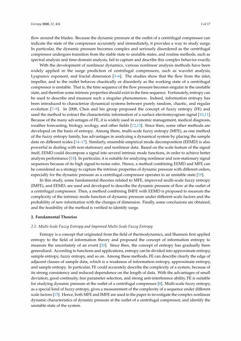
in Figure 7. Similarly, the scale factor τ is set from 1 to 10, and the analysis unit is one second.From Figure 7, we see that the tendencies of the curves of IMFE are consistent with those of MFE.Compared with the curves in Figure 5, the curves of IMFE show less overlap, and the differencesbetween curves for different scale factors are seen more clearly. Therefore, IMFE is more suitable thanMFE to analyze the nonlinear characteristics of the dynamic pressure.


Figure 7, we see that the tendencies of the curves of IMFE are consistent with those of MFE. Compared with the curves in Figure 5, the curves of IMFE show less overlap, and the differences between curves for different scale factors are seen more clearly. Therefore, IMFE is more suitable than MFE to analyze the nonlinear characteristics of the dynamic pressure.

Figure 7. IMFE of dynamic pressure throughout the time period.

Then, the relationship between IMFE and scale factor τ for the dynamic pressure at the outlet is analyzed. In Figure 8, the same six time periods as in Figure 6 are used. In contrast with the curves of MFE, the values of IMFE are largest for the stable stage and smallest for the surge state for all scale factors, the curves under the different states are smooth, the curves decrease with the increase of the scale factor for all three states and there is no intersection between curves for different states. Therefore, IMFE makes it easier to identify the different working states of a centrifugal compressor. Furthermore, it can be drawn that IMFE is a much more reliable solution to analyzing the characteristics of the centrifugal compressor in different states, because the values of entropies of the stable state and transition state are very close, as the scale factor is one.

Figure 8. IMFE of dynamic pressure under different scale factors.

In order to improve the anti-noise, EEMD combined with IMFE is used in this study. First, the time sequence of the dynamic pressure is decomposed by EEMD, and then the resulting IMF components are analyzed by IMFE in the following section.

5. IMFE Combined with EEMD of Dynamic Pressure

5.1. EEMD Decomposition of Dynamic Pressure

As shown in Figure 4, 100 s data including the stable, transition, and surge states of the centrifugal compressor are decomposed by EEMD. According to the definition and decomposition method of EEMD, the results of EEMD decomposition are not only related to the signal itself, but also depend closely on the amplitude and times of the white noise that is added after several experiments,


Then, the relationship between IMFE and scale factor τ for the dynamic pressure at the outlet isanalyzed. In Figure 8, the same six time periods as in Figure 6 are used. In contrast with the curvesof MFE, the values of IMFE are largest for the stable stage and smallest for the surge state for allscale factors, the curves under the different states are smooth, the curves decrease with the increaseof the scale factor for all three states and there is no intersection between curves for different states.Therefore, IMFE makes it easier to identify the different working states of a centrifugal compressor.Furthermore, it can be drawn that IMFE is a much more reliable solution to analyzing the characteristicsof the centrifugal compressor in different states, because the values of entropies of the stable state andtransition state are very close, as the scale factor is one.


Figure 7, we see that the tendencies of the curves of IMFE are consistent with those of MFE. Compared with the curves in Figure 5, the curves of IMFE show less overlap, and the differences between curves for different scale factors are seen more clearly. Therefore, IMFE is more suitable than MFE to analyze the nonlinear characteristics of the dynamic pressure.


Then, the relationship between IMFE and scale factor τ for the dynamic pressure at the outlet is analyzed. In Figure 8, the same six time periods as in Figure 6 are used. In contrast with the curves of MFE, the values of IMFE are largest for the stable stage and smallest for the surge state for all scale factors, the curves under the different states are smooth, the curves decrease with the increase of the scale factor for all three states and there is no intersection between curves for different states. Therefore, IMFE makes it easier to identify the different working states of a centrifugal compressor. Furthermore, it can be drawn that IMFE is a much more reliable solution to analyzing the characteristics of the centrifugal compressor in different states, because the values of entropies of the stable state and transition state are very close, as the scale factor is one.


In order to improve the anti-noise, EEMD combined with IMFE is used in this study. First, the time sequence of the dynamic pressure is decomposed by EEMD, and then the resulting IMF components are analyzed by IMFE in the following section.



As shown in Figure 4, 100 s data including the stable, transition, and surge states of the centrifugal compressor are decomposed by EEMD. According to the definition and decomposition method of EEMD, the results of EEMD decomposition are not only related to the signal itself, but also depend closely on the amplitude and times of the white noise that is added after several experiments,


In order to improve the anti-noise, EEMD combined with IMFE is used in this study. First, the timesequence of the dynamic pressure is decomposed by EEMD, and then the resulting IMF componentsare analyzed by IMFE in the following section.



As shown in Figure 4, 100 s data including the stable, transition, and surge states of the centrifugalcompressor are decomposed by EEMD. According to the definition and decomposition method

Entropy 2020, 22, 424 9 of 17

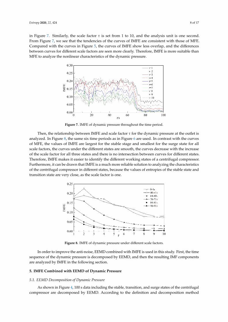
of EEMD, the results of EEMD decomposition are not only related to the signal itself, but alsodepend closely on the amplitude and times of the white noise that is added after several experiments,the amplitude of white noise is set as 0.05 PSI. EEMD decomposition of the data is shown in Figure 9,including six IMF components and a residual component. From Figure 9, it can be seen that IMF1,IMF2, and IMF3 could not describe the change of the operating state of the centrifugal compressor.IMF4 could reflect the transition state, but it only weakly distinguishes the stable state from the surgestate. Among them, IMF6 could clearly distinguish the stable state from the surge state; however,the transition state is not obvious for this component. As for IMF5, it appears to amplify fluctuation ofthe dynamic pressure, especially for the stable state.


the amplitude of white noise is set as 0.05 PSI. EEMD decomposition of the data is shown in Figure 9, including six IMF components and a residual component. From Figure 9, it can be seen that IMF1, IMF2, and IMF3 could not describe the change of the operating state of the centrifugal compressor. IMF4 could reflect the transition state, but it only weakly distinguishes the stable state from the surge state. Among them, IMF6 could clearly distinguish the stable state from the surge state; however, the transition state is not obvious for this component. As for IMF5, it appears to amplify fluctuation of the dynamic pressure, especially for the stable state.

Figure 9. Ensemble empirical mode decomposition (EEMD) decomposition of dynamic pressure. Figure 9. Ensemble empirical mode decomposition (EEMD) decomposition of dynamic pressure.

Entropy 2020, 22, 424 10 of 17

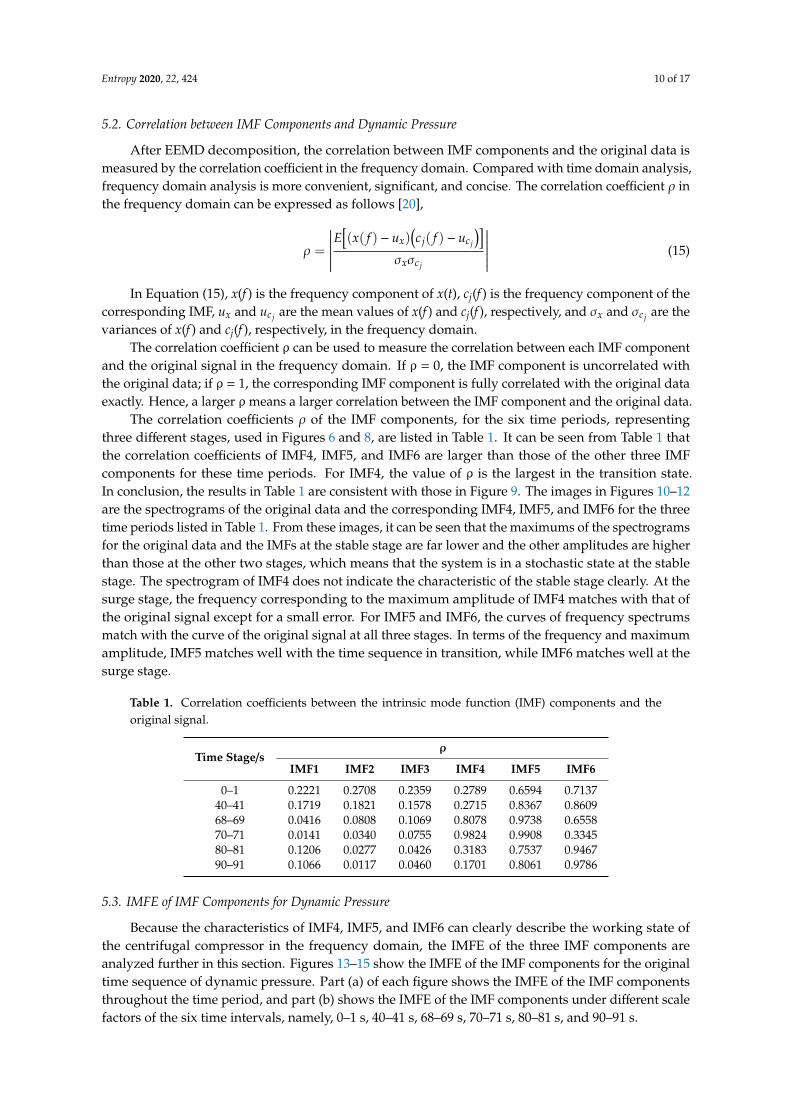
5.2. Correlation between IMF Components and Dynamic Pressure

After EEMD decomposition, the correlation between IMF components and the original data ismeasured by the correlation coefficient in the frequency domain. Compared with time domain analysis,frequency domain analysis is more convenient, significant, and concise. The correlation coefficient ρ inthe frequency domain can be expressed as follows [20],

ρ =

∣∣∣∣∣∣∣E[(x( f ) − ux)

(c j( f ) − uc j

)]σxσc j

∣∣∣∣∣∣∣ (15)

In Equation (15), x(f ) is the frequency component of x(t), cj(f ) is the frequency component of thecorresponding IMF, ux and uc j are the mean values of x(f ) and cj(f ), respectively, and σx and σc j are thevariances of x(f ) and cj(f ), respectively, in the frequency domain.

The correlation coefficient ρ can be used to measure the correlation between each IMF componentand the original signal in the frequency domain. If ρ = 0, the IMF component is uncorrelated withthe original data; if ρ = 1, the corresponding IMF component is fully correlated with the original dataexactly. Hence, a larger ρ means a larger correlation between the IMF component and the original data.

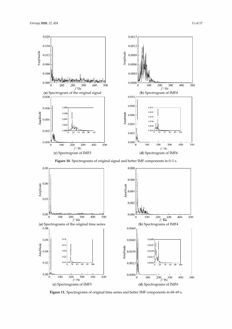
The correlation coefficients ρ of the IMF components, for the six time periods, representingthree different stages, used in Figures 6 and 8, are listed in Table 1. It can be seen from Table 1 thatthe correlation coefficients of IMF4, IMF5, and IMF6 are larger than those of the other three IMFcomponents for these time periods. For IMF4, the value of ρ is the largest in the transition state.In conclusion, the results in Table 1 are consistent with those in Figure 9. The images in Figures 10–12are the spectrograms of the original data and the corresponding IMF4, IMF5, and IMF6 for the threetime periods listed in Table 1. From these images, it can be seen that the maximums of the spectrogramsfor the original data and the IMFs at the stable stage are far lower and the other amplitudes are higherthan those at the other two stages, which means that the system is in a stochastic state at the stablestage. The spectrogram of IMF4 does not indicate the characteristic of the stable stage clearly. At thesurge stage, the frequency corresponding to the maximum amplitude of IMF4 matches with that ofthe original signal except for a small error. For IMF5 and IMF6, the curves of frequency spectrumsmatch with the curve of the original signal at all three stages. In terms of the frequency and maximumamplitude, IMF5 matches well with the time sequence in transition, while IMF6 matches well at thesurge stage.

Table 1. Correlation coefficients between the intrinsic mode function (IMF) components and theoriginal signal.

Time Stage/sρ

IMF1 IMF2 IMF3 IMF4 IMF5 IMF6

0–1 0.2221 0.2708 0.2359 0.2789 0.6594 0.713740–41 0.1719 0.1821 0.1578 0.2715 0.8367 0.860968–69 0.0416 0.0808 0.1069 0.8078 0.9738 0.655870–71 0.0141 0.0340 0.0755 0.9824 0.9908 0.334580–81 0.1206 0.0277 0.0426 0.3183 0.7537 0.946790–91 0.1066 0.0117 0.0460 0.1701 0.8061 0.9786

5.3. IMFE of IMF Components for Dynamic Pressure

Because the characteristics of IMF4, IMF5, and IMF6 can clearly describe the working state ofthe centrifugal compressor in the frequency domain, the IMFE of the three IMF components areanalyzed further in this section. Figures 13–15 show the IMFE of the IMF components for the originaltime sequence of dynamic pressure. Part (a) of each figure shows the IMFE of the IMF componentsthroughout the time period, and part (b) shows the IMFE of the IMF components under different scalefactors of the six time intervals, namely, 0–1 s, 40–41 s, 68–69 s, 70–71 s, 80–81 s, and 90–91 s.

Entropy 2020, 22, 424 11 of 17


(a) Spectrogram of the original signal (b) Spectrogram of IMF4

(c) Spectrogram of IMF5 (d) Spectrogram of IMF6

Figure 10. Spectrograms of original signal and better IMF components in 0–1 s.

(a) Spectrograms of the original time series (b) Spectrograms of IMF4

(c) Spectrograms of IMF5 (d) Spectrograms of IMF6

Figure 11. Spectrograms of original time series and better IMF components in 68–69 s.



(a) Spectrogram of the original signal (b) Spectrogram of IMF4

(c) Spectrogram of IMF5 (d) Spectrogram of IMF6




Figure 11. Spectrograms of original time series and better IMF components in 68–69 s. Figure 11. Spectrograms of original time series and better IMF components in 68–69 s.

Entropy 2020, 22, 424 12 of 17Entropy 2019, 21, x FOR PEER REVIEW 12 of 17



Figure 12. Spectrograms of original time series and better IMF components in 90–91 s.

5.3. IMFE of IMF Components for Dynamic Pressure

Because the characteristics of IMF4, IMF5, and IMF6 can clearly describe the working state of the centrifugal compressor in the frequency domain, the IMFE of the three IMF components are analyzed further in this section. Figures 13–15 show the IMFE of the IMF components for the original time sequence of dynamic pressure. Part (a) of each figure shows the IMFE of the IMF components throughout the time period, and part (b) shows the IMFE of the IMF components under different scale factors of the six time intervals, namely, 0–1 s, 40–41 s, 68–69 s, 70–71 s, 80–81 s, and 90–91 s.

From Figure 13a, it can be seen that the curves of IMFE for IMF4 collapse at 68 s and IMFE increases sharply at 75 s. The values of IMFE are small for the time stage 68–75 s, as the centrifugal compressor operates in the transition state. From Figure 14a, it is clear that the variation of curves of IMFE for IMF5 in the stable state is larger than in the surge state, but the variation is not obvious for the transition state. In Figure 15a, the curves collapse at 75 s, and the changing of the curves of IMFE for IMF6 is contrary to that of IMFE for IMF4. As the system operates in surge state, the variation is very low and the values of IMFE are small for IMF6. As a result, it can be concluded that IMFE of IMF4 could exactly distinguish the transition state, and IMFE of IMF6 can be used to predict the occurrence of surge.

From part (b) of Figures 13–15, similar to the IMFE of dynamic pressure in Figures 7 and 8, the different working states of the centrifugal compressor can be identified clearly. Moreover, compared with Figure 8, the differences in IMFE of the IMF components are more obvious than the IMFE of dynamic pressure under most scale factors. Furthermore, it is easy to identify the transition state in the IMFE of IMF4, since the separation between stable state and unstable state is obvious. Similarly, the obvious separation occurs in transition, identified by the IMFE of IMF6. However, for the IMFE of IMF5, the separation occurs just before the transition, therefore the IMFE of IMF5 is more suitable to predict the surge than the IMFE of IMF6 in terms of dynamic pressure at the outlet.

Since each of IMFEs of IMF components can indicate a certain characteristic, it is significant to study the nonlinear characteristics of the dynamic pressure using IMFE of IMF components.

Figure 12. Spectrograms of original time series and better IMF components in 90–91 s.Entropy 2019, 21, x FOR PEER REVIEW 13 of 17

(a) IMFE of IMF4 throughout the time period (b) IMFE of IMF4 under different scale factors

Figure 13. IMFE of IMF4 for original time sequence.





6. Statistical Reliability of IMFE of IMF Components for Dynamic Pressure

In order to test the statistical reliability of the IMFE of IMF components, the data of dynamic pressure are modified by adding randomly shuffled data. According the maximum absolute data of the dynamic pressure, white noise with an amplitude of 0.02 PSI is chosen as the randomly shuffled data. EEMD decomposition of the randomly shuffled dynamic pressures is shown in Figure 16, including six IMF components and a residual component R. The same conclusion is drawn from Figure 16 as from Figure 9, which infers that the noise has no influence on the analysis result obtained from the method.


From Figure 13a, it can be seen that the curves of IMFE for IMF4 collapse at 68 s and IMFEincreases sharply at 75 s. The values of IMFE are small for the time stage 68–75 s, as the centrifugalcompressor operates in the transition state. From Figure 14a, it is clear that the variation of curves ofIMFE for IMF5 in the stable state is larger than in the surge state, but the variation is not obvious forthe transition state. In Figure 15a, the curves collapse at 75 s, and the changing of the curves of IMFEfor IMF6 is contrary to that of IMFE for IMF4. As the system operates in surge state, the variation isvery low and the values of IMFE are small for IMF6. As a result, it can be concluded that IMFE of IMF4could exactly distinguish the transition state, and IMFE of IMF6 can be used to predict the occurrenceof surge.

Entropy 2020, 22, 424 13 of 17





















From part (b) of Figures 13–15, similar to the IMFE of dynamic pressure in Figures 7 and 8,the different working states of the centrifugal compressor can be identified clearly. Moreover,compared with Figure 8, the differences in IMFE of the IMF components are more obvious than theIMFE of dynamic pressure under most scale factors. Furthermore, it is easy to identify the transitionstate in the IMFE of IMF4, since the separation between stable state and unstable state is obvious.Similarly, the obvious separation occurs in transition, identified by the IMFE of IMF6. However, for theIMFE of IMF5, the separation occurs just before the transition, therefore the IMFE of IMF5 is moresuitable to predict the surge than the IMFE of IMF6 in terms of dynamic pressure at the outlet.

Since each of IMFEs of IMF components can indicate a certain characteristic, it is significant tostudy the nonlinear characteristics of the dynamic pressure using IMFE of IMF components.


In order to test the statistical reliability of the IMFE of IMF components, the data of dynamicpressure are modified by adding randomly shuffled data. According the maximum absolute data of thedynamic pressure, white noise with an amplitude of 0.02 PSI is chosen as the randomly shuffled data.EEMD decomposition of the randomly shuffled dynamic pressures is shown in Figure 16, including sixIMF components and a residual component R. The same conclusion is drawn from Figure 16 as fromFigure 9, which infers that the noise has no influence on the analysis result obtained from the method.

Entropy 2020, 22, 424 14 of 17Entropy 2019, 21, x FOR PEER REVIEW 14 of 17

Figure 16. IMF components and residual component of shuffled flow pressure.

Figures 17–19 show IMFE of the IMF components for the shuffled dynamic pressure. Part (a) of each figures shows the IMFE of IMF components throughout the time period, and part (b) shows the comparison of the original and randomly shuffled dynamic pressure in IMFE of the IMF components, under different scale factors for the six time intervals, at 0–1 s, 40–41 s, 68–69 s, 70–71 s, 80–81 s, and 90–91 s. Moreover, the variation in the IMFE of IMF components shows properties consistent with the results for the original time sequence. In part (b) in Figures 17–19, the curves also show consistent properties graphically with the curves of part (b) in Figures 13–15, except for small errors.

Figure 16. IMF components and residual component of shuffled flow pressure.

Figures 17–19 show IMFE of the IMF components for the shuffled dynamic pressure. Part (a) ofeach figures shows the IMFE of IMF components throughout the time period, and part (b) shows thecomparison of the original and randomly shuffled dynamic pressure in IMFE of the IMF components,under different scale factors for the six time intervals, at 0–1 s, 40–41 s, 68–69 s, 70–71 s, 80–81 s,and 90–91 s. Moreover, the variation in the IMFE of IMF components shows properties consistent with

Entropy 2020, 22, 424 15 of 17

the results for the original time sequence. In part (b) in Figures 17–19, the curves also show consistentproperties graphically with the curves of part (b) in Figures 13–15, except for small errors.Entropy 2019, 21, x FOR PEER REVIEW 15 of 17


Figure 17. IMFE of IMF4 for shuffled time sequence.





7. Conclusions

In this study, as a powerful measure method for entropy, MFE, and IMFE of the dynamic pressure at the outlet of a centrifugal compressor was studied to obtain intrinsic properties. The results show that IMFE can exactly describe the complexity and the probability of the dynamic pressure under different scale factors. Specifically, the MFE and IMFE of the dynamic pressure decrease and become smooth as the system enters surge from the stable state, and the method of IMFE is more effective than that of MFE at certain scale factors. After studying the data, the results of the IMFE analysis of IMF components can provide detailed information regarding dynamic pressure in the frequency domain, because a slight fluctuation in the stable state and transition state









7. Conclusions










7. Conclusions



7. Conclusions

In this study, as a powerful measure method for entropy, MFE, and IMFE of the dynamic pressureat the outlet of a centrifugal compressor was studied to obtain intrinsic properties. The results showthat IMFE can exactly describe the complexity and the probability of the dynamic pressure underdifferent scale factors. Specifically, the MFE and IMFE of the dynamic pressure decrease and become

Entropy 2020, 22, 424 16 of 17

smooth as the system enters surge from the stable state, and the method of IMFE is more effective thanthat of MFE at certain scale factors. After studying the data, the results of the IMFE analysis of IMFcomponents can provide detailed information regarding dynamic pressure in the frequency domain,because a slight fluctuation in the stable state and transition state could be revealed clearly in differentIMF components. After analyzing the shuffled dynamic pressure, the results show that the methodproposed in this study has certain anti-noise values and can be well-applied to the prediction anddetection of surge for a centrifugal compressor. The subsequent work will use the results to accuratelypredict the initial surge of a centrifugal compressor, in order to prevent surge development.

Author Contributions: Conceptualization, Writing—Review & Editing, Y.L.; Simulation, Writing—Original DraftPreparation, K.M.; Data Acquisition, K.G.; Visualization, H.H. All authors have read and agreed to the publishedversion of the manuscript.

Funding: This research is supported by National Natural Science Foundation of China (No. 51775437 and No.51305355) and State Key Laboratory of Compressor Technology of China (No. SKL-YSJ201902).

Acknowledgments: We thank LetPub (www.LetPub.com) for its linguistic assistance during the preparation ofthis manuscript; The authors acknowledge Xi’an Shaangu Power Co., Ltd. for the data used in this paper.

Conflicts of Interest: The authors declare no conflict of interest.

References

1. Sorokes, J.M.; Kuzdzal, M.J. Centrifugal compressor evolution. Compress. Blower Fan Technol. 2011, 3, 61–67.2. Wang, X.J.; Ge, L.L.; Tan, J.J. The Development Process of Centrifugal Compressor and the Future Technology

Development Trend in China. Compress. Blower Fan Technol. 2015, 3, 65–77.3. Ma, J. Research on Analysis and Prediction of Compressor Unstable Signal Based on Orthogonal Wavelet.

Master’s Thesis, Nanjing University of Aeronautics and Astronautics, Nanjing, China, 2010.4. Liu, Y.; Chen, D.M.; Liu, L.G.; Wang, H.; Cheng, K. Exploring mono-fractal characteristics of dynamic

pressure at exit of centrifugal compressor. J. Northwestern Polytech. Univ. 2013, 31, 60–66.5. Liu, Y.; Zhang, J.Z. Predicting Traffic Flow in Local Area Networks by the Largest Lyapunov Exponent.

Entropy 2016, 18, 32. [CrossRef]6. Liu, Y.; Ding, D.X.; Ma, K. Descriptions of entropy with fractal dynamics and their applications to the flow

pressure of centrifugal compressor. Entropy 2019, 21, 266. [CrossRef]7. Pincus, S.M. Approximate entropy as a measure of system complexity. Proc. Natl. Acad. Sci. USA 1991,

88, 2297–2301. [CrossRef]8. Richman, J.S.; Moorman, J.R. Physiological time-series analysis using approximate entropy and sample

entropy. Am. J. Physiol. Heart Circ. Physiol. 2000, 278, 2039–2049. [CrossRef]9. Guariglia, E. Entropy and Fractal Antennas. Entropy 2016, 18, 84. [CrossRef]10. Chen, W.T. A Study of Feature Extraction from SEMG Signal Based on Entropy. Ph.D. Thesis, Shanghai Jiao

Tong University, Shanghai, China, 2008.11. Chen, W.T.; Zhuang, J.; Yu, W.X.; Wang, Z.Z. Measuring complexity using FuzzyEn, ApEn, and SampEn.

Med. Eng. Phys. 2009, 31, 61–68. [CrossRef]12. Liu, H.; Xie, H.B.; He, W.X. Characterization and classification of EEG sleep stage based on fuzzy entropy.

J. Data Acquis. Process. 2010, 25, 484–489.13. Hu, J.F.; Wang, T.T. Analysis of driving fatigue detection based on fuzzy entropy of EEG signals. China Saf.

Sci. J. 2018, 28, 13–18.14. Costa, M.D.; Goldberger, A.L. Generalized multiscale entropy analysis: Application to quantifying the

complex volatility of human heartbeat time series. Entropy 2015, 17, 1197–1203. [CrossRef]15. Costa, M.D.; Goldberger, A.L.; Peng, C.K. Multiscale entropy analysis of biological signals. Phys. Rev. E 2005,

71, 021906. [CrossRef] [PubMed]16. Lee, K.Y.; Wang, C.C.; Lin, S.G.; Wu, C.W.; Wu, S.D. Time Series Analysis Using Composite Multiscale

Entropy. Entropy 2013, 15, 1069–1084.17. Zheng, J.D.; Pan, H.Y.; Zhang, J.; Liu, T.; Liu, Q.Y. Multivariate multiscale fuzzy entropy based planetary

gearbox fault diagnosis. J. Vib. Meas. Diagn. 2019, 38, 187–193.

www.LetPub.com

http://dx.doi.org/10.3390/e18010032

http://dx.doi.org/10.3390/e21030266

http://dx.doi.org/10.1073/pnas.88.6.2297

http://dx.doi.org/10.1152/ajpheart.2000.278.6.H2039

http://dx.doi.org/10.3390/e18030084

http://dx.doi.org/10.1016/j.medengphy.2008.04.005

http://dx.doi.org/10.3390/e17031197

http://dx.doi.org/10.1103/PhysRevE.71.021906

http://www.ncbi.nlm.nih.gov/pubmed/15783351

Entropy 2020, 22, 424 17 of 17

18. Wu, Z.; Huang, N.E. Ensemble empirical mode decomposition: A noise assisted data analysis method.Adv. Adapt. Data Anal. 2008, 1, 1–41. [CrossRef]

19. Zhao, H.M.; Sun, M.; Deng, W.; Yang, X.H. A new feature extraction method based on EEMD and multi-scalefuzzy entropy for motor bearing. Entropy 2016, 19, 14–35. [CrossRef]

20. Humeau-Heurtier, A. The multiscale entropy algorithm and its variants: A review. Entropy 2015, 17, 3110–3123.[CrossRef]

21. Zheng, J.D.; Dai, J.X.; Zhu, X.L.; Pan, H.Y.; Pan, Z.W. A Rolling Bearing Fault Diagnosis Approach Based onImproved Multiscale Fuzzy Entropy. J. Vib. Meas. Diagn. 2018, 38, 929–934.

22. Ju, B.; Zhang, H.J.; Liu, Y.B.; Liu, F.; Lu, S.L.; Dai, Z.J. A feature extraction method using improved multi-scaleentropy for rolling bearing fault diagnosis. Entropy 2018, 20, 212. [CrossRef]

23. Hamed, A.; Javier, E. Improved multiscale permutation entropy for biomedical signal analysis: Interpretationand application to electroencephalogram recordings. Biomed. Signal Process Control 2016, 23, 28–41.

24. Hamed, A.; Alberto, F.; Javier, E. Refined multiscale fuzzy entropy based on standard deviation for biomedicalsignal analysis. Med. Biol. Eng. Comput. 2017, 55, 2037–2052.

© 2020 by the authors. Licensee MDPI, Basel, Switzerland. This article is an open accessarticle distributed under the terms and conditions of the Creative Commons Attribution(CC BY) license (http://creativecommons.org/licenses/by/4.0/).

http://dx.doi.org/10.1142/S1793536909000047

http://dx.doi.org/10.3390/e19010014

http://dx.doi.org/10.3390/e17053110

http://dx.doi.org/10.3390/e20040212

http://creativecommons.org/

http://creativecommons.org/licenses/by/4.0/.

centrifugal compressor from pressure by combining eemd and

Documents