cfd-caa coupled calculations of a tandem cylinder ... · the cfd-caa coupling is based on cfd data...

CFD-CAA Coupled Calculations of a Tandem Cylinder Configuration to Assess Facility Installation Effects

Stéphane Redonnet1 ONERA (French Aerospace Centre), BP 72 - 29 av Division Leclerc, Châtillon, 92322, France

David P. Lockard2, Mehdi R. Khorrami3, Meelan M. Choudhari3 NASA Langley Research Center, MS 128, Hampton, VA 23681-2199

This paper presents a numerical assessment of acoustic installation effects in the tandem cylinder (TC) experiments conducted in the NASA Langley Quiet Flow Facility (QFF), an open-jet, anechoic wind tunnel. Calculations that couple the Computational Fluid Dynamics (CFD) and Computational Aeroacoustics (CAA) of the TC configuration within the QFF are conducted using the CFD simulation results previously obtained at NASA LaRC. The coupled simulations enable the assessment of installation effects associated with several specific features in the QFF facility that may have impacted the measured acoustic signature during the experiment. The CFD-CAA coupling is based on CFD data along a suitably chosen surface, and employs a technique that was recently improved to account for installed configurations involving acoustic backscatter into the CFD domain. First, a CFD-CAA calculation is conducted for an ‘isolated TC configuration’ to assess the coupling approach, as well as to generate a reference solution for subsequent assessments of QFF installation effects. Direct comparisons between the CFD-CAA calculations associated with the various installed configurations allow the assessment of the effects of each component (nozzle, collector, etc.) or feature (confined vs. free jet flow, etc.) characterizing the NASA LaRC QFF facility.

Nomenclature

f = frequency

fprim = primary shedding frequency

λprim = wavelength of the primary shedding acoustic emission M = Mach number

p’ = pressure perturbation

PSD = Power Spectral Density

r = radial distance to the acoustic source position t = time coordinate

Tprim = primary shedding period

x,y,z = Cartesian coordinates

R = cylinder radius

I. Introduction

he noise environment around airports is a major concern in the world, with many local communities exposed to

high levels of aircraft noise. Effective reduction of such ‘noise pollution’ represents an important environmental

challenge for the foreseeable future. The noise signature of an aircraft includes two main contributors; namely, the

engine noise component, which includes noise radiation from both turbomachinery (fan, turbine, combustion, etc.)

and the jet, as well as an airframe (or aerodynamic) noise component attributed to the interaction between turbulent

flow over the airframe and the adjacent solid structures, such as wings, slats, flaps, landing gears and cavities, etc.

1 PhD, Research scientist, CFD and Aeroacoustics Department, ONERA. 2 Research scientist, Computational AeroSciences Branch, Senior Member, AIAA. 3 Research scientist, Computational AeroSciences Branch, Associate Fellow, AIAA.

T

https://ntrs.nasa.gov/search.jsp?R=20110015465 2018-11-07T09:23:16+00:00Z

American Institute of Aeronautics and Astronautics

2

Although engine noise accounts for a dominant portion of the overall aircraft noise during take-off, the airframe

noise component becomes equally important during the approach for landing, when the engine thrust is considerably

reduced. In their effort to develop quieter airplanes, aircraft manufacturers need to design airframes that minimize

the intensity of flow induced acoustic radiation to the far field. Consequently, the development of capabilities that

offer both a deeper understanding and an accurate prediction of the physical phenomena related to aerodynamic

noise generation and propagation mechanisms has became a priority for the aerospace research community. In particular, numerical simulations have emerged as a valuable complement to the more traditional experimental

methods.

II. Aerodynamic Noise Prediction and Hybrid Approaches

Prediction of aerodynamic noise is a complex problem that includes physical phenomena over a broad range of spatio-temporal scales. More precisely, the generation of acoustic disturbances is driven by turbulent structures of

high amplitude and small space-time correlations, while the propagation of the acoustic disturbances is characterized

by waves of low amplitude and large space-time correlations. Although both phenomena are ruled by the same

compressible Navier-Stokes equations, they cannot be easily predicted via a single calculation because the

computational resources required to resolve all of the relevant scales would be far too high. To make the numerical

approach tractable in a practical context, the overall aeroacoustic problem is therefore decomposed into a set of

coupled subproblems that focus on individual subregions of the overall spatial domain. Each subproblem has a

specific range of amplitudes and physical scales that can be addressed using a numerical method that is customized

to the dominant physics in that subregion. Methods involving a mixture of techniques in this manner are classified

as hybrid methods for aeroacoustic prediction.

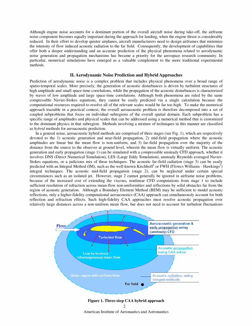
In a general sense, aeroacoustic hybrid methods are comprised of three stages (see Fig. 1), which are respectively devoted to the 1) acoustic generation and near-field propagation, 2) mid-field propagation where the acoustic

amplitudes are linear but the mean flow is non-uniform, and 3) far-field propagation over the majority of the

distance from the source to the observer at ground level, wherein the mean flow is virtually uniform. The acoustic

generation and early propagation (stage 1) can be simulated with a compressible unsteady CFD approach, whether it

involves DNS (Direct Numerical Simulation), LES (Large Eddy Simulation), unsteady Reynolds averaged Navier-

Stokes equations, or a judicious mix of these techniques. The acoustic far-field radiation (stage 3) can be easily

predicted with an Integral Method (IM), such as the well-known Kirchhoff1 or FWH (Ffowcs Williams - Hawkings2)

integral techniques. The acoustic mid-field propagation (stage 2), can be neglected under certain special

circumstances such as an isolated jet. However, stage 2 cannot generally be ignored in airframe noise problems,

because of the increased cost of extending the viscous, nonlinear CFD computations from stage 1 to include

sufficient resolution of refraction across mean-flow non-uniformities and reflections by solid obstacles far from the region of acoustic generation. Although a Boundary Element Method (BEM) may be sufficient to model acoustic

reflections, only a higher-fidelity computational aeroacoustics (CAA) approach can simultaneously account for both

reflection and refraction effects. Such high-fidelity CAA approaches must resolve acoustic propagation over

relatively large distances across a non-uniform mean flow, but does not need to account for turbulent fluctuations

Figure 1. Three-step CAA hybrid approach


3

and, perhaps, even viscous effects on acoustic propagation. This may typically be accomplished with the Euler

equations or a linearized version thereof.

A critical aspect of developing such hybrid methodologies corresponds to the coupling, i.e., the information

exchange, between the prediction modules for individual stages. The nature of this coupling is problem dependent,

because of significant variations in the interdependencies between the various stages from one problem to another.

However, except in problems involving acoustic feedback (e.g. screech tones), the coupling between the various stages is weak, i.e., primarily unidirectional3. Under this scenario, feedback from a given stage to the previous one

can then be neglected.

Implementing an appropriate one-way coupling from the unsteady CFD to the CAA stage is an essential

ingredient in hybrid aeroacoustic methods that seek to simulate the full cycle of events associated with a complex

aerodynamic noise problem, ranging from near-field generation to far-field radiation and including the mid-field

propagation. As discussed in Ref. 3, derivation of such coupling is a challenging task. In particular, such a coupling

has to ensure that all acoustic events generated in stage 1 as part of the CFD simulation will be correctly transmitted

to the CAA solver for stage 2 without any loss or duplication of the acoustic sources. Currently, at least two

approaches for coupling CFD and CAA solvers exist, namely those based on 1) volumetric and 2) surface coupling.

Initially developed at ONERA4, the CFD-CAA surface coupling was successfully applied to several practical

airframe noise applications5-7 such as acoustic emission by both an in-flight NACA0012 airfoil with a blunted

trailing edge and a thick plate embedded within a flow. Very recently, the technique was improved further3 to deal with installed configurations; more precisely, the coupling process was modified to be transparent to the propagation

of acoustic waves reflected back through the coupling interface – an event likely to occur whenever installed

configurations are considered, since solid bodies surrounding the source region can reflect back anything the latter

radiates. Such a CFD-CAA surface coupling technique was extensively used within the present effort, so as to

enable coupled calculations of the noise emitted by a Tandem Cylinder configuration including installation effects.

III. CFD-CAA Calculations of the Tandem Cylinder Configuration

The present section is devoted to the Tandem Cylinder configuration and the results of applying the CFD/CAA

surface coupling technique to this configuration.

A. Background

To better understand some of the generic physical mechanisms associated with landing gear noise sources, a

combined experimental and computational campaign was carried out at NASA Langley Research Center, focusing

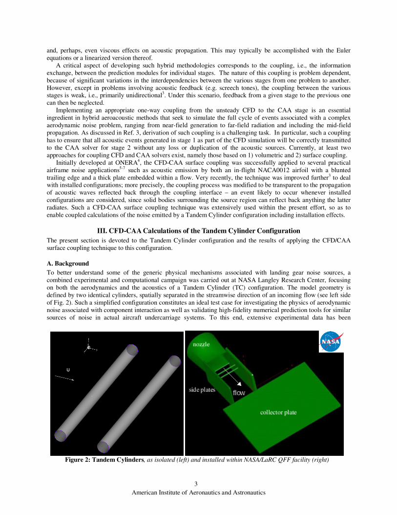
on both the aerodynamics and the acoustics of a Tandem Cylinder (TC) configuration. The model geometry is

defined by two identical cylinders, spatially separated in the streamwise direction of an incoming flow (see left side

of Fig. 2). Such a simplified configuration constitutes an ideal test case for investigating the physics of aerodynamic

noise associated with component interaction as well as validating high-fidelity numerical prediction tools for similar

sources of noise in actual aircraft undercarriage systems. To this end, extensive experimental data has been

Figure 2: Tandem Cylinders, as isolated (left) and installed within NASA/LaRC QFF facility (right)


4

collected8-11 and compared to the results of 3-D, unsteady CFD computations12,13. Despite the favorable

comparison between the measured and computed spectra, a legitimate concern existed about some of the obvious

differences occurring between the installed TC configuration that had been tested and the simplified configuration

that was computed. In other words, questions arose about the fact that these calculations did not incorporate any of

the possible installation effects that could have occurred in the experiments. Indeed, as indicated previously,

accounting for all or part of the installation components (e.g., QFF side plates) during the initial CFD stage would have been far too expensive, requiring a fine mesh to compute not only the cylinders, but also the side walls

supporting / surrounding them. In addition, the intrinsic limitations of Helmoltz-based integral methods2 limit the

FWH stage from correctly accounting for reflections / diffraction and the convection / refraction effects that may be

caused by the QFF itself and its confined jet flow. Therefore, a numerical assessment of the acoustic reflection /

diffraction effects of the main components of the anechoic facility (see right side of Fig. 2) was conducted a

posteriori14 with an Equivalent Source Model (ESM) approach and solver (Fast Scattering Code)15. There was,

however, both a need and an interest to go further in such an a posteriori assessment of possible acoustic installation

effects characterizing the TC acoustic experiments, by improving the fidelity of the acoustic propagation stage; first,

it was desirable to account for the acoustic emission that had been effectively generated (or, at least, predicted by the

CFD stage), rather than to model it via equivalent sources. Second, it seemed important to account not only for the

reflection / diffraction effects induced by the experimental apparatus in the anechoic facility, but also for the

(partial) convection / refraction effects characterizing its (confined and sheared) jet flow. These two requirements could obviously be fulfilled by a CFD-CAA coupled approach such as the one previously described, especially

considering that its recent improvement enabled it to properly handle all acoustic propagation back through the

coupling surface that was expected to occur in such an 'installed' situation. Consequently, several CFD-CAA

coupled calculations of the installed TC configuration were conducted, all of which were 1) performed using the

CFD-CAA surface coupling technique, and 2) based on the same CFD data12,13 (coming from the isolated TC

computations initially performed at NASA LaRC). The near-field data was obtained using the second-order, Navier-

Stokes CFD code CFL3D and a hybrid RANS/LES turbulence model. The computations were performed with a 13

million node grid with periodic boundary conditions in the spanwise direction. Only the geometry of the cylinders

was included in the configuration. The span used in the computations was 18 cylinder diameters. For additional

details on the simulations, the reader is referred to Refs. 12 and 13.

B. Preliminary Activities

Before a CAA computation could be conducted, a

number of preliminary (though non-trivial) tasks were

required.

III.B.1 CAA grid generation

The first task consisted of generating proper CAA grids of the TC configuration, which had to be considered as

both isolated and (partially) installed. Several meshes

were thus derived via analytical means, all being

targeted to capture correctly acoustic waves up to a

frequency of 400 Hz. Targeting such a (low) frequency

was both justified by the characteristics of the primary

shedding frequency (f’prim = 220 Hz), and imposed by

the sampling rate with which CFD simulation data had

been stored. With a total of 28 blocks and comprised of

0.85 millions cells, the largest grid incorporated all the

main features of the QFF (side plates, collector plate, jet nozzle – see Fig. 3), which were slightly approximated

when the modifications would not adversely affect the

accuracy of the simulations. First, the nozzle shape was

simplified. That is, its slightly curved panels were

replaced by straight ones. Then, considering their

thickness could reasonably be neglected for such a low

frequency source, both the nozzle and the side plates

were modeled as infinitely thin. Finally, with the view

of minimizing the CPU cost, the lateral (z) dimension of Figure 3. CAA mesh of the fully installed TC


5

the computational domain was restricted to include only 2/3rd of the collector plate’s spanwise extent. Given that the

thickness of the collector had the potential to be non-negligible, the collector plate was meshed without

approximation with special attention being paid to its rounded leading edge. The xy plane computational domain was

extended beyond the microphones, so that the CFD-CAA outputs could be directly compared to the CFD/FWH

results initially obtained at those microphone locations12,13. Finally, in all the regions where a better spatial

resolution was desired, the CAA grid density was locally and in a progressive manner refined. In particular, the grid in the source region, in the vicinity of jet shear layers, and around the plates' edges were made denser (by a factor of

7). Because the grid was generated analytically, smoothness of the grid and metrics could be assured to be greater

than the order of the CAA solver. Although the grid was not systematically refined, the grid spacing was chosen to

resolve the important range of frequencies in the problem based on the demonstrated resolving capability of the

CAA code4, 5, 16. Furthermore, some grid sensitivity studies were performed, and the results were found to be

relatively insensitive to refinement beyond the grid spacing used in this study.

III.B.2 Derivation of both the mean flow and the CAA forcing

A second preliminary task consisted of constructing the requisite base flow field (comprised of both the steady mean

flow field for the perturbed Euler equations, and an associated instantaneous perturbed counterpart to be used in the

forcing term in the CAA computation), before interpolating them onto the CAA grid. For this reconstruction,

although available steady flow data (coming from RANS calculations) could have been used, the choice was made to generate a stationary field by time-averaging all the successive instantaneous CFD computed flow realizations

that had been stored. This was dictated by a legitimate concern to preserve the formulation's consistency, which

requires consistently defining both the mean and the perturbed quantities over the source region. Once the

construction of the mean flow was achieved, all the fluctuating components corresponding to such a steady mean

flow were calculated by subtracting the latter from the total field. Those decomposed mean and perturbed flow fields

were then interpolated in space from the CFD to CAA grid using a (tri) linear process. Once interpolated onto the

CAA grid, these steady mean and instantaneous perturbed flow fields had to be subjected to a few additional

manipulations; first, since the CAA computational domain was extended beyond the CFD domain boundaries, the

steady mean flow field was extrapolated and the missing data were algebraically reconstructed wherever needed.

Then, the steady mean flow was smoothed out by successive applications of second order spatial filters. The main

reason for doing so was to prevent insufficient grid resolution of the viscous mean flow gradients in the vicinity of the cylinders in the Euler-type CAA grid, which would have led to numerical instabilities. For the same reason, the

boundary layers surrounding the cylinder surfaces were removed from the CAA mean flow, and a special treatment

was applied to avoid large gaps between the values at the wall and the first point off the wall. The treatment

involved overwriting the near wall values by extrapolating radially from the interior of the CAA domain, just

outside the boundary layers .

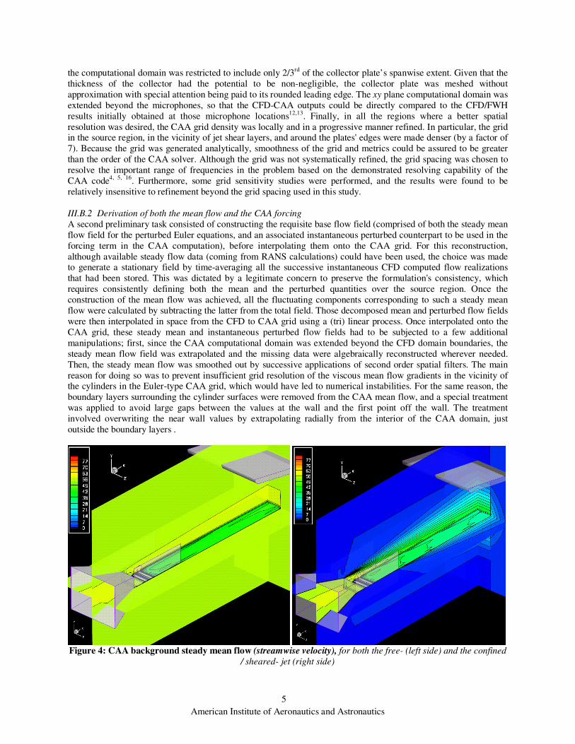
Figure 4: CAA background steady mean flow (streamwise velocity), for both the free- (left side) and the confined

/ sheared- jet (right side)


6

Two different steady mean flows for the CAA calculation were derived; the first one was directly inherited from

the CFD computational data set, providing a 'free-field' mean flow that matched the CFD steady values at infinity

(for a free stream Mach number of 0.166 – see left side of Fig. 4). First, concerning the isolated TC configuration,

such a free jet mean flow enabled a direct comparison with the CFD-FWH results, in order to validate further the

coupling procedure itself. For the installed TC configuration, such a free-jet mean flow provided a reference solution against which results associated with a more realistic steady jet flow could be compared, allowing an assessment of

convection / refraction effects of the QFF jet shear layers. One can notice that - as is - this extrapolated free jet flow

was partly unrealistic, with a slightly non physical flow behavior occurring in the vicinity of both the nozzle and the

collector. However, in the absence of a more suitable definition (which would have required performing a steady

CFD calculation of the entire QFF configuration), and since no major issues were expected (just a few minor

reflection / refraction errors), this background jet mean flow was used as is.

To improve the underlying physics, a second mean flow was derived with the aim of better representing the

experimental conditions. In reality, the jet flow is initially confined within the nozzle walls. As the jet exits the

nozzle into the ambient air, free shear layers develop at the nozzle lips, spreading out with axial distance. Acoustic

waves can be refracted or deflected by such shear layers, modifying the directivity pattern. Similarly, the absence of

any convection outside the jet may lead to propagation patterns that differ from the ones associated with the free-jet

flow previously presented. Therefore, the latter was modified via analytical means using similarity functions to obtain a more realistic mean flow with jet spreading effects (see right side of Fig. 4). The functions were derived for

spatial evolution at a rate driven by both 1) the x-axial distance to the nozzle exit plane and 2) the y- / z- lateral

distance to the nozzle lips. The jet spreading rate was calibrated to match experimental observations in the QFF,

corresponding to a spreading angle of 7o. Once properly derived, this 'confined / sheared' mean flow was further

modified analytically to exhibit more realistic streamline patterns within the nozzle area.

The instantaneous perturbed flow field, having been interpolated in space between the CFD and CAA grids, was

subjected to two additional manipulations. First, it was interpolated in time because the maximum time step

compatible with the CAA grid was 35 times smaller than the one used for storing the CFD data. Although more

advanced techniques could have been used, the data was linearly interpolated in time. This was achieved directly

during the CAA calculation; the CAA solver internally reconstructed the temporal signals from two successive steps

of CFD data. The second manipulation of the instantaneous perturbed flow field consisted of multiplying the forcing terms by a function that transitioned smoothly from unity around the cylinders to zero downstream of the rear

cylinder. This was achieved in order to prevent the cylinder’s wake from interacting with both 1) the aft part of the

surface coupling interface and 2) the downstream boundary of the CAA domain.

Regardless of whether the steady mean flow was considered 'free' or 'confined / sheared,' the same set of

instantaneous perturbed quantities was prescribed to be injected into the CAA calculation. This was done so that the

acoustic source would be free of any bias possibly induced by different mean / perturbed splitting definitions.

Furthermore, this was justified by theoretical considerations which indicate that as long as a perturbation problem

remains linear, the fluctuating field is independent of the mean state (except for refraction effects). Finally, one can

notice that from an aero/acoustic point of view, the Tandem Cylinders are neither fully isolated nor fully installed.

Indeed, in order to simplify the treatment of the spanwise boundaries, the CFD employed periodic conditions,

allowing aero/acoustic signals to be recycled in the spanwise direction. Consequently, the resulting perturbed fields

could neither be considered as physically truncated nor bounded in the lateral direction - which would have been required for the CAA calculations to be formally isolated or installed. However, a CFD calculation of the installed

configuration would have required excessive computer resources. Furthermore, the change in geometry could have

altered the near-field source in an unpredictable manner making it difficult for the CAA to separate out the effects of

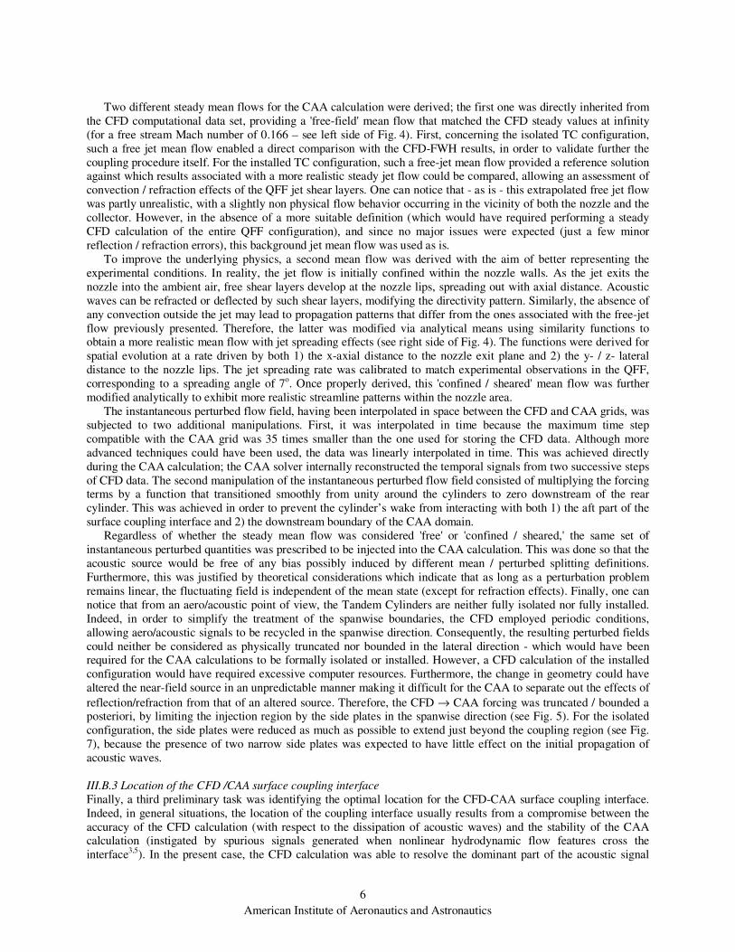
reflection/refraction from that of an altered source. Therefore, the CFD → CAA forcing was truncated / bounded a posteriori, by limiting the injection region by the side plates in the spanwise direction (see Fig. 5). For the isolated

configuration, the side plates were reduced as much as possible to extend just beyond the coupling region (see Fig.

7), because the presence of two narrow side plates was expected to have little effect on the initial propagation of

acoustic waves.

III.B.3 Location of the CFD /CAA surface coupling interface

Finally, a third preliminary task was identifying the optimal location for the CFD-CAA surface coupling interface.

Indeed, in general situations, the location of the coupling interface usually results from a compromise between the

accuracy of the CFD calculation (with respect to the dissipation of acoustic waves) and the stability of the CAA calculation (instigated by spurious signals generated when nonlinear hydrodynamic flow features cross the

interface3,5). In the present case, the CFD calculation was able to resolve the dominant part of the acoustic signal


7

well into the near field because the bulk of the energy was at very

low frequencies. However, using a coupling surface far from the

cylinders would not have allowed the CAA computation to include

the effects of reflection/diffraction from the side plates inside of the

coupling surface. Consequently, for consistency more than for

accuracy reasons, the coupling interface was located as close to the cylinders as possible without getting into regions of strong

hydrodynamic activity (see Fig. 5) which would violate the

assumption of linear disturbances underlying the hybrid

methodology and also require a finer grid density in the CAA mesh

to resolve viscous flow features3.

C. Computed Cases and Set-Up

III.C.1 Computed cases

For the first calculation the TC configuration was considered as

isolated, i.e. free of any installation effects. This case provided a

reference solution against which results obtained for the various

installed configurations could be compared in order to assess the

specific reflection/diffraction and/or convection/refraction effects characterizing each configuration. Another

objective was to validate further the CFD-CAA surface coupling approach, by comparing the results with the ones

initially obtained by NASA LaRC researchers, who had computed the isolated TC case via a CFD/FWH

approach12,13. Obviously, for such an isolated case, the ‘free jet’ steady mean flow obtained from the CFD was

imposed in the CAA calculation.

Additional calculations were performed for the installed configurations, first with the free-jet steady mean flow used for the isolated case (see left side of Fig. 4). Doing so was motivated by the desire to assess the reflection /

diffraction effects independently from convection / refraction. To estimate separately the reflection / diffraction

effects of each QFF component (side plates, collector plate,

nozzle), additional calculations were conducted, with components

added successively.

Finally, a last calculation focused on the more realistic case,

i.e. the fully QFF-installed TC associated with the corresponding

confined / sheared jet mean flow (see right side of Fig. 4). This

calculation aimed not only at delivering still higher-fidelity

results, but also at highlighting all possible convection / refraction

effects characterizing the mean flow.

III.C.2 Computational set up

All the CAA calculations were conducted with ONERA’s

sAbrinA.v0 solver3-7, 16-18, using NASA computational resources.

sAbrinA.v0 is a structured grid, time-accurate CAA code that

solves the full Euler equations, either in a conservative form or

non-conservative, perturbed form (with a splitting of the complete

variables into a ‘frozen’ mean flow and a ‘fluctuating’

perturbation). The solver employs high-order, finite-difference

operators, involving 6th-order spatial derivatives and 10th-order

filters, as well as a 6th-order, multi-stage, Runge-Kutta time-

marching scheme. The code deals with multi-block structured grids with one-to-one interfaces, and is fully parallelized using the

Message Passing Interface (MPI) standard. Finally, the solver

includes the usual boundary conditions (reflection by solid walls,

non-reflecting, free-field radiation4,6, etc.), as well some unique to

specific applications (such as the surface coupling technique that

was extensively used in the present effort). The surface coupling

technique consists of an implicit forcing of the CAA field, driven

by instantaneous perturbed quantities previously obtained via

analytical or numerical means (e.g. a CFD calculation). This

Figure 5: CFD-CAA surface coupling

interface (in blue)

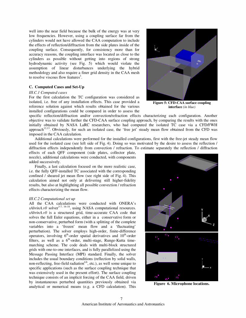
Figure 6. Microphone locations.


8

technique has been described and validated in Ref 3. More detailed information about the sAbrinA.v0 solver and its

underlying methodology can be found in Refs. 4 and 16.

All calculation cases were computed in parallel, via 64 processors on a PC cluster at NASA Langley Research

Center. Calculations were run for a number of time steps covering the temporal extent of the CFD data record,

corresponding to approximately 20 periods of the primary shedding frequency. The CAA grid and mean flow for

each case were adjusted to properly model the effects of relevant components (i.e., scattering agents) within the QFF. The fully installed configuration used 28 domains, and only a subset of the 28 domains was used for the other

cases involving fewer scattering components. As previously stated, the source from the CFD data imposed on the

coupling surface in the CAA simulations was kept identical for all cases. The source distribution based on each

stored time step of the CFD database was linearly interpolated to the appropriate time in the CAA simulation, and

injected within the CAA computational domain via the surface coupling forcing. For all cases, the entire

instantaneous perturbed pressure field was stored at regular intervals during the calculation. The perturbed pressure

signal time history was also stored and post-processed (to obtain the power spectral density) at specific points

corresponding to the microphone locations in the experiment (see Fig. 6). Finally, both the RMS (root mean square)

perturbed pressure field and the acoustic phase field associated with the primary shedding frequency (f’prim) were

determined from the computations.

III.C.3 CPU performance

Depending on the size of the CAA grid used for each case (between 530,000 cells for the isolated TC, and 853,000

cells for the fully installed TC), all calculations required between 11h and 18h of wall clock time on 64 CPUs.

Scaled to the number of CAA iterations (12,600) and cores (64) involved indicates an average CPU time of

approximately 384 µsec/iteration/cell/core. This (quite poor) CPU performance was mainly due to three factors; first, the I/O operations needed for both reading the CFD data and storing the CAA outputs were numerous and

unoptimized. The performance penalty (of approximately 25%) was accepted to allow greater flexibility in choosing

what information to read and write. Secondly, these 0.5 to 0.8 million cell cases were not the best candidates for

efficient distribution over 64 cores because there were twice as many ghost cells (requiring data exchanges across

the network) as a serial computation. Although clearly not optimal, the parallel decomposition of the cases was

nevertheless conducted, considering that it still resulted in a significant reduction in the time to solution. Finally, the

Intel P4 2.53 CPUs used are now relatively old, and a more modern cluster can achieve significantly better

performance; when run on 64-bit Itanium processors with a high-speed interconnect, similar calculations produced

CPU times of approximately 50

µsec/iteration/cell/core.

D. Isolated TC in a Free-Jet Flow

The TC configuration was first considered as

being as close to isolated as possible, i.e. free of

any installation devices, with its steady mean

flow being derived in a 'free-jet' sense.

III.D.1 Calculation results and early analysis

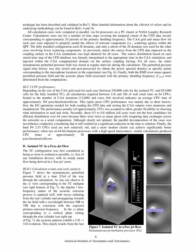
Figure 7 shows the instantaneous perturbed

pressure field at a time 2/3rd of the way

through the calculation. As one can observe in

the xy view corresponding to the TC midspan

(see right bottom of Fig. 7), the dipolar / low-

frequency nature of the acoustic emission

process is captured well, with waves radiating

from the rear cylinder and propagating towards

the far field with a wavelength between 30R to

35R that is consistent with the expected primary emission frequency. In the yz plane

corresponding to a vertical plane cutting

through the rear cylinder (see right top

of Fig. 7), the acoustic patterns exhibit a 2-D →

3-D evolution. This clearly results from the fact Figure 7. Isolated TC in a free jet flow. Instantaneous perturbation pressure (Pa)


9

that, after their injection into the CAA computational domain and initial propagation within the bounded region that

the cylinders span, the acoustic waves lose the quasi 2-D features inherited from the underlying CFD. These

observations were confirmed by the investigation of both the RMS perturbed pressure field and the phase fronts

corresponding to a frequency of f’prim (not shown here); the dipolar nature of the acoustic radiation was clearly

visible, as well as the progression from 2D → 3D of the contour patterns; in the near field, acoustic fronts seemed

'flatter' in the yz plane than in xy, while in the far field, they all had roughly the same curvature.

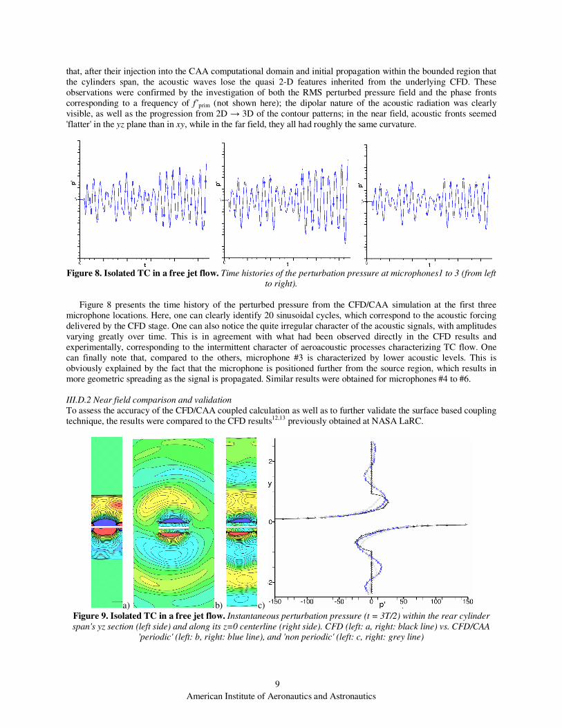
Figure 8. Isolated TC in a free jet flow. Time histories of the perturbation pressure at microphones1 to 3 (from left

to right).

Figure 8 presents the time history of the perturbed pressure from the CFD/CAA simulation at the first three

microphone locations. Here, one can clearly identify 20 sinusoidal cycles, which correspond to the acoustic forcing

delivered by the CFD stage. One can also notice the quite irregular character of the acoustic signals, with amplitudes

varying greatly over time. This is in agreement with what had been observed directly in the CFD results and

experimentally, corresponding to the intermittent character of aeroacoustic processes characterizing TC flow. One

can finally note that, compared to the others, microphone #3 is characterized by lower acoustic levels. This is

obviously explained by the fact that the microphone is positioned further from the source region, which results in

more geometric spreading as the signal is propagated. Similar results were obtained for microphones #4 to #6.

III.D.2 Near field comparison and validation

To assess the accuracy of the CFD/CAA coupled calculation as well as to further validate the surface based coupling

technique, the results were compared to the CFD results12,13 previously obtained at NASA LaRC.

a) b) c)

Figure 9. Isolated TC in a free jet flow. Instantaneous perturbation pressure (t = 3T/2) within the rear cylinder

span's yz section (left side) and along its z=0 centerline (right side). CFD (left: a, right: black line) vs. CFD/CAA

'periodic' (left: b, right: blue line), and 'non periodic' (left: c, right: grey line)


10

Such a comparison is problematic because both calculations were not exactly representative of the same

configuration; indeed, the CFD calculation was run with spanwise periodic boundary conditions producing a nearly

2-D radiation pattern, with waves fronts progressing almost horizontally (see Fig. 9a).However, in the CAA

calculation, the source region is embedded in an unbounded region, allowing the acoustic waves to adopt a 3-D

propagation behavior, where they rapidly loose their 2-D features initially inherited from the CFD stage (see Fig.

9b). Direct comparison of results led to the observation that, although both amplitudes matched exactly at the

surface coupling interface (see right side of Fig. 9), the CFD/CAA signal was weaker than in the CFD counterpart –

which could partly be explained by the fact that acoustic propagation is characterized by a different spreading rate in

2D (1/√r) than in 3D (1/r). Therefore, an alternative CFD/CAA calculation of the isolated TC configuration was

conducted, which aimed at better matching with the CFD numerical set-up; hence, all CAA domains extending

beyond the cylinders in the spanwise direction were truncated and lateral periodic boundary conditions applied. This

led to CFD/CAA matching better with the CFD, both in terms of the general pattern and amplitude, with a resulting

perturbed pressure field characterized by a more spanwise uniform behavior, and acoustic waves with horizontal

wave fronts and increased levels (see Fig. 9c). However, as one can see, some discrepancies still remain between

both calculations, and their exact origin is still unclear. One possible explanation could be the inability of the CFD

stage to accurately account for the near-field prediction of acoustic waves. In particular, although the CFD solver

should be capable of accurately propagating such a low-frequency signal relatively accurately over such a short

distance, the large wavelength presents a challenge to non-reflecting boundary conditions, and the CFD calculation employed a simple Riemann boundary condition that may have resulted in significant reflections compared with the

more advanced boundary conditions used in the CAA code.

Another possibility involves an uncertainty regarding the CFD → CAA interpolation process, which - in the present

case - had to be conducted not only in time, but also in space. Indeed, according to ongoing theoretical studies being

conducted at ONERA19, any CFD → CAA interpolation process may be subject to various spurious phenomena

(spectral aliasing, etc.), which can result in the emergence of errors within the CAA stage. Although all such

possible CFD → CAA interpolation issues are not completely identified, one can expect that their effects would be

minimal for the very low-frequency character of this particular acoustic problem. Whatever the reasons for the

discrepancies between the CFD and the CFD/CAA near fields, it is important to remember that CAA methods

generally offer higher fidelity/flexibility than CFD in dealing with acoustic phenomena. Consequently, the

discrepancies observed here may not indicate any problems with the coupling technique, but instead that the combined CFD/CAA approach may be able to more faithfully simulate configurations of interest. In particular, this

suggests that the present CFD/CAA hybrid approach could be used to correct the CFD/FWH results not only from

physical artifacts (here the QFF acoustic installation effects), but also from some purely methodological

approximations employed for computational simplicity (e.g. periodic boundary conditions that were employed in the

CFD simulations).

III.D.3 Far-field comparison and validation

Because of the difficulty in directly comparing the CFD/CAA near-field to its CFD counterpart, far-field

comparisons were made employing the FWH solver used to estimate the isolated TC acoustic signature at

microphones #1 to #3.

Figure 10. Isolated TC in a free-jet flow. Power Spectral Density of the perturbation pressure

propagated/radiated to microphones 1 to 3 (from left to right). CFD/CAA (in blue) vs. CFD/FWH (in black)

The CFD/FWH spectra12 were compared to those computed from time history signals sampled directly from the


11

CFD/CAA computational domain (see Fig. 8). For each of the first three microphones, Fig. 10 displays the PSD

(Power Spectral Density) from both the CFD/FWH and CFD/CAA calculations; although their absolute levels do

not match exactly, both spectra have the same trends (over a frequency range extending beyond those well resolved -

see section II.B.1), and exhibit the same tonal peak at f = 212 Hz (which corresponds to fprim, to within the Fast

Fourier Transform (FFT) bandwidth of 10Hz). Despite the overall agreement in the spectra, they also exhibit some

discrepancies, for which various explanations can be proposed. First, for all three microphones, the agreement between the CFD/CAA and CFD/FWH spectra degrades beyond 400Hz. This can obviously be attributed to the fact

that such a 400Hz limit corresponds to the highest frequency for which a good resolution was ensured by the CAA

grid. Second, considering the three plots successively reveals that the divergence between the CFD/FWH and

CFD/CAA spectra seems to be more pronounced for microphone #3, located downstream of the cylinders. This

could be due to spurious effects from the coupling interface caused by the passage of hydrodynamic events

convected by the wake. Indeed, in the present case, the function used to artificially confine the forcing to the vicinity

of the cylinders could have been insufficient to prevent all (intermittent and relatively strong) hydrodynamic events

from corrupting the downstream section of the coupling interface. Furthermore, the CFD/FWH and the CFD/CAA

spectra exhibit an amplitude mismatch at the tonal frequency. Such an amplitude mismatch cannot be associated

with the inability of the CFD stage to accurately account for the near-field acoustic propagation since, in the present

case, only the solid surface data from the CFD was used in the FWH calculation. In the same way, such amplitude

discrepancies cannot be attributed to the inability of this FWH/solid surface computation to account for possible quadrupole noise sources, since alternative FWH/porous surface calculations have been conducted that produced no

real difference in the far-field results. However, a possible reason for the mismatch in amplitude could be because

the periodic boundary conditions in the CFD calculation imposed perfect spanwise correlation at both cylinders'

extremities. Consequently, the FWH extrapolation could have produced a non-negligible over-estimation of acoustic

levels in the mid-span plane, precisely where the microphones are located. Finally, the differences in amplitude

levels could also have been associated with the FWH-related FFT post-processes.

Therefore, in an effort to make the procedures for calculating the far-field noise as close as possible between the

two simulations, the CFD/CAA data was used as input to the FWH solver and compared with the CFD/FWH

computed signals.

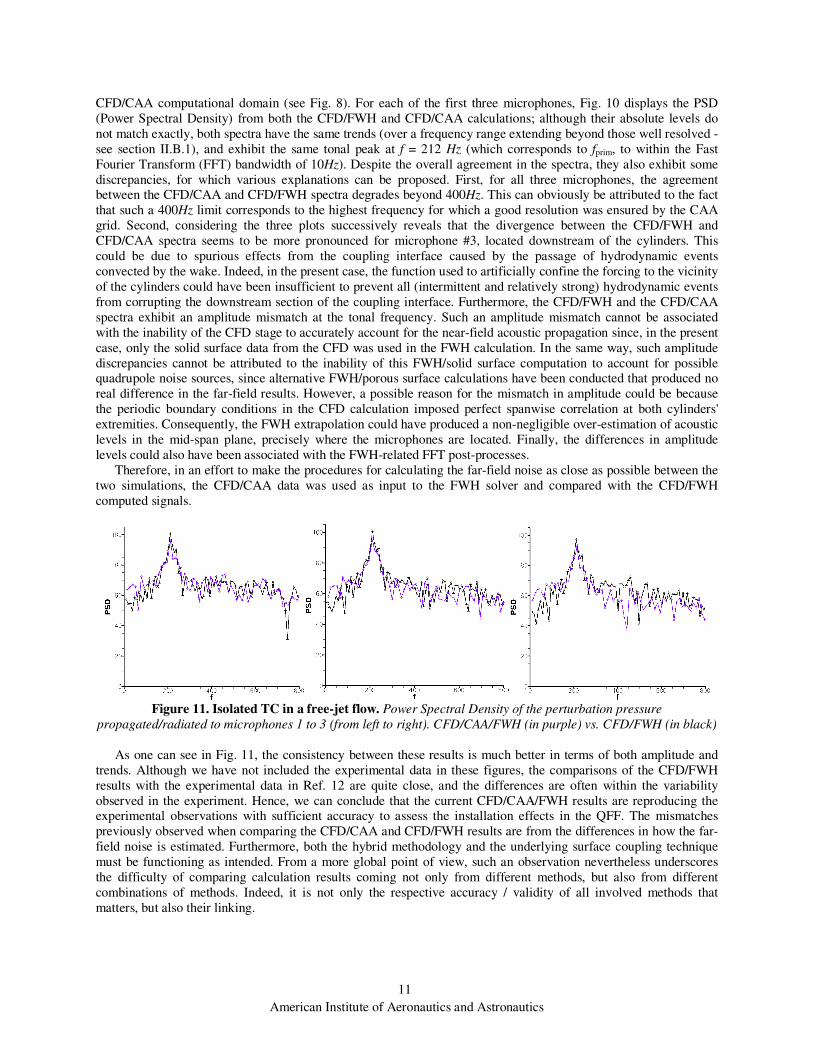
Figure 11. Isolated TC in a free-jet flow. Power Spectral Density of the perturbation pressure

propagated/radiated to microphones 1 to 3 (from left to right). CFD/CAA/FWH (in purple) vs. CFD/FWH (in black)

As one can see in Fig. 11, the consistency between these results is much better in terms of both amplitude and

trends. Although we have not included the experimental data in these figures, the comparisons of the CFD/FWH

results with the experimental data in Ref. 12 are quite close, and the differences are often within the variability

observed in the experiment. Hence, we can conclude that the current CFD/CAA/FWH results are reproducing the experimental observations with sufficient accuracy to assess the installation effects in the QFF. The mismatches

previously observed when comparing the CFD/CAA and CFD/FWH results are from the differences in how the far-

field noise is estimated. Furthermore, both the hybrid methodology and the underlying surface coupling technique

must be functioning as intended. From a more global point of view, such an observation nevertheless underscores

the difficulty of comparing calculation results coming not only from different methods, but also from different

combinations of methods. Indeed, it is not only the respective accuracy / validity of all involved methods that

matters, but also their linking.


12

E. Installed TC in a Free-Jet Flow

To isolate the reflection / diffraction effects produced by the QFF experimental setup on the TC acoustic signature,

the previous isolated configuration was modified to include the main QFF elements (side plates, collector plate,

nozzle), with the steady mean flow still being considered as a free jet (see left side of Fig. 4).

III.E.1 Calculation results and early analysis

Views of the instantaneous perturbation pressure field are presented in Fig. 12, at a time 2/3rd of the way through

the calculation. A comparison between these results and those from the isolated TC configuration (see Fig. 7)

reveals that the QFF devices modify the acoustic field in several ways. First, between the side plates, acoustic waves

exhibit an enhanced 2-D character, as well as

increased amplitudes. This can be attributed to the

partial confinement that acoustic waves experience. Indeed, once generated, acoustic waves are trapped on

two sides by the side plates, which then act on them

as a wave guide. Secondly, outside of the side plates,

acoustic waves display an enhanced 3-D character,

while they exhibit higher amplitudes between the

plates (especially in the mid-span yz plane, compare

right/top views of Figs. 7 and 12). The change from

2D → 3D in the propagation behavior occurs when

acoustic waves are diffracted by the side plates' edges,

which 'break up' the initial 2-D character of emitted

waves, promoting a 3-D / free space propagation behavior. Finally, further away from the side plates,

acoustic waves maintain their 3-D nature, with either

slightly higher or lower amplitudes, depending on the

location. As will be shown, such relative gains /

losses in amplitude seem to result primarily from the

cumulative effect of all QFF components, which

cause constructive / destructive interference on the

overall acoustic field. These various acoustic

installation effects appear even more explicitly when

comparing the present acoustic phase field to its

isolated TC counterpart (see Fig. 13). First, one can

notice the higher curvature that acoustic wave fronts adopt in the yz plane, which reflects the transition

from 2-D → 3-D propagation that the side plates

enhance. Furthermore, a direct comparison of other

views reveals how both the collector plate and the

nozzle modify the acoustic patterns in their immediate

vicinity, as revealed by the strong discontinuities

characterizing the acoustic phase field (and thus wave

fronts) nearby these obstacles. These local

modifications of the acoustic phase by the solid obstacles indirectly indicate the reflection / diffraction phenomena,

which can have a more global impact due to the backscatter of acoustic waves into the domain. Cumulatively, all

these effects might explain the amplitude changes that the acoustic field exhibits throughout the domain, as indicated by the comparison of both RMS perturbed pressure fields (not shown here).

III.E.2 Further assessment of acoustic installation effects by QFF components

To more clearly identify the origin of all various acoustic installation effects occurring here, three RMS 'delta' maps

were produced, which are presented in Fig. 14. These maps were calculated from the RMS perturbed pressure fields

associated with each of the various 'installed TC' configurations successively computed. The configuration without

any QFF components was taken as the baseline, and the sequence of simulations highlights the differences in RMS

levels in the acoustic field when the QFF components were progressively installed. Consequently, these delta maps

indicate the respective contribution of each QFF component (side plates, collector plate and nozzle, successively) to

the overall acoustic installation effects; the left side of Fig. 14 confirms that the side plates primarily contribute to a

Figure 12. Installed TC in a free jet flow. Instantaneous perturbation pressure (Pa)


13

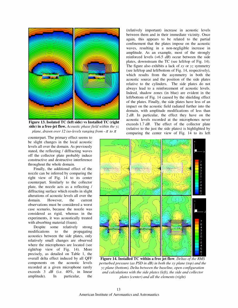
(relatively important) increase in acoustic levels

between them and in their immediate vicinity. Once

again, this appears to be related to the partial

confinement that the plates impose on the acoustic

waves, resulting in a non-negligible increase in

amplitude. As an example, most of the strongly reinforced levels (+6.5 dB) occur between the side

plates, downstream the TC (see left/top of Fig. 14).

The figure also exhibits a lack of xy or yz symmetry

(see left/top and left/bottom of Fig. 14, respectively),

which results from the asymmetry in both the

acoustic source and the position of the side plates

relative to the cylinders. The side plates do not

always lead to a reinforcement of acoustic levels.

Indeed, shadow zones (in blue) are evident in the

left/bottom of Fig. 14 caused by the shielding effect

of the plates. Finally, the side plates have less of an

impact on the acoustic field radiated further into the domain, with amplitude modifications of less than

2 dB. In particular, the effect they have on the

acoustic levels recorded at the microphones never

exceeds 1.7 dB. The effect of the collector plate

(relative to the just the side plates) is highlighted by

comparing the center view of Fig. 14 to its left

counterpart. The primary effect seems to

be slight changes in the local acoustic

levels all over the domain. As previously

stated, the reflecting / diffracting waves

off the collector plate probably induce constructive and destructive interference

throughout the whole domain.

Finally, the additional effect of the

nozzle can be inferred by comparing the

right view of Fig. 14 to its center

counterpart. Similarly to the collector

plate, the nozzle acts as a reflecting /

diffracting surface which results in slight

alterations of acoustic levels all over the

domain. However, the current

observations must be considered a worst

case scenario, because the nozzle was considered as rigid, whereas in the

experiments, it was acoustically treated

with absorbing material (foam).

Despite some relatively strong

modifications to the propagating

acoustics between the side plates, only

relatively small changes are observed

where the microphones are located (see

right/top view of Fig. 14). More

precisely, as detailed on Table 1, the

overall delta effect induced by all QFF components on the acoustic levels

recorded at a given microphone rarely

exceeds 3 dB (i.e. 40%, in linear

amplitude). In particular, the

Figure 14. Installed TC within a free jet flow. Deltas of the RMS

perturbed pressure (as PSD in dB) in both the xy plane (top) and the

yz plane (bottom). Delta between the baseline, open configuration

and calculations with the side plates (left), the side and collector

plates (center) and all the elements (right)

Figure 13. Isolated TC (left side) vs Installed TC (right side) in a free-jet flow. Acoustic phase field within the yz

plane, drawn over 12 iso-levels ranging from –π to π


14

microphones located just downstream of the cylinders (mics #2 and #5) are the ones for which the overall acoustic

installation effects are the weakest. For some microphones, adding a particular QFF component may mitigate the

effect induced by others devices (for example, the effect of the nozzle on mics #1, #4 and #5). Furthermore, the

lower microphones (mics #4 to #6) are subjected to similar changes in the acoustic levels as the upper ones (mics #1

to #3), although they are located further away from the collector plate. These two observations indicate that each

microphone is subject to a global cumulative influence of all QFF components, rather than to a local effect induced by the closest QFF component. In other words, the acoustic installation effects appear to be driven by the

constructive and destructive interference from the cumulative reflection / diffraction off of all the QFF components.

In addition, both the observer's location and the acoustic source dynamics play an important role. This behavior is to

be expected because of the very low-frequency character of the noise source, make it relatively non-compact with

respect to the experimental set up. From an acoustic installation point of view, the various QFF devices interact

quite closely, and cannot really be considered separately.

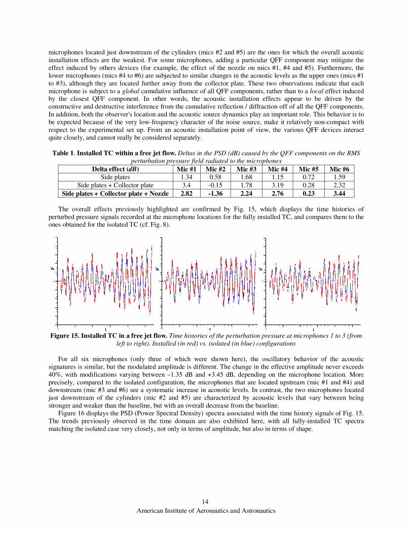
Table 1. Installed TC within a free jet flow. Deltas in the PSD (dB) caused by the QFF components on the RMS

perturbation pressure field radiated to the microphones

Delta effect (dB) Mic #1 Mic #2 Mic #3 Mic #4 Mic #5 Mic #6 Side plates 1.34 0.58 1.68 1.15 0.72 1.59

Side plates + Collector plate 3.4 -0.15 1.78 3.19 0.28 2.32

Side plates + Collector plate + Nozzle 2.82 -1.36 2.24 2.76 0.23 3.44

The overall effects previously highlighted are confirmed by Fig. 15, which displays the time histories of

perturbed pressure signals recorded at the microphone locations for the fully installed TC, and compares them to the ones obtained for the isolated TC (cf. Fig. 8).

Figure 15. Installed TC in a free jet flow. Time histories of the perturbation pressure at microphones 1 to 3 (from

left to right). Installed (in red) vs. isolated (in blue) configurations

For all six microphones (only three of which were shown here), the oscillatory behavior of the acoustic

signatures is similar, but the modulated amplitude is different. The change in the effective amplitude never exceeds

40%, with modifications varying between –1.35 dB and +3.45 dB, depending on the microphone location. More

precisely, compared to the isolated configuration, the microphones that are located upstream (mic #1 and #4) and downstream (mic #3 and #6) see a systematic increase in acoustic levels. In contrast, the two microphones located

just downstream of the cylinders (mic #2 and #5) are characterized by acoustic levels that vary between being

stronger and weaker than the baseline, but with an overall decrease from the baseline.

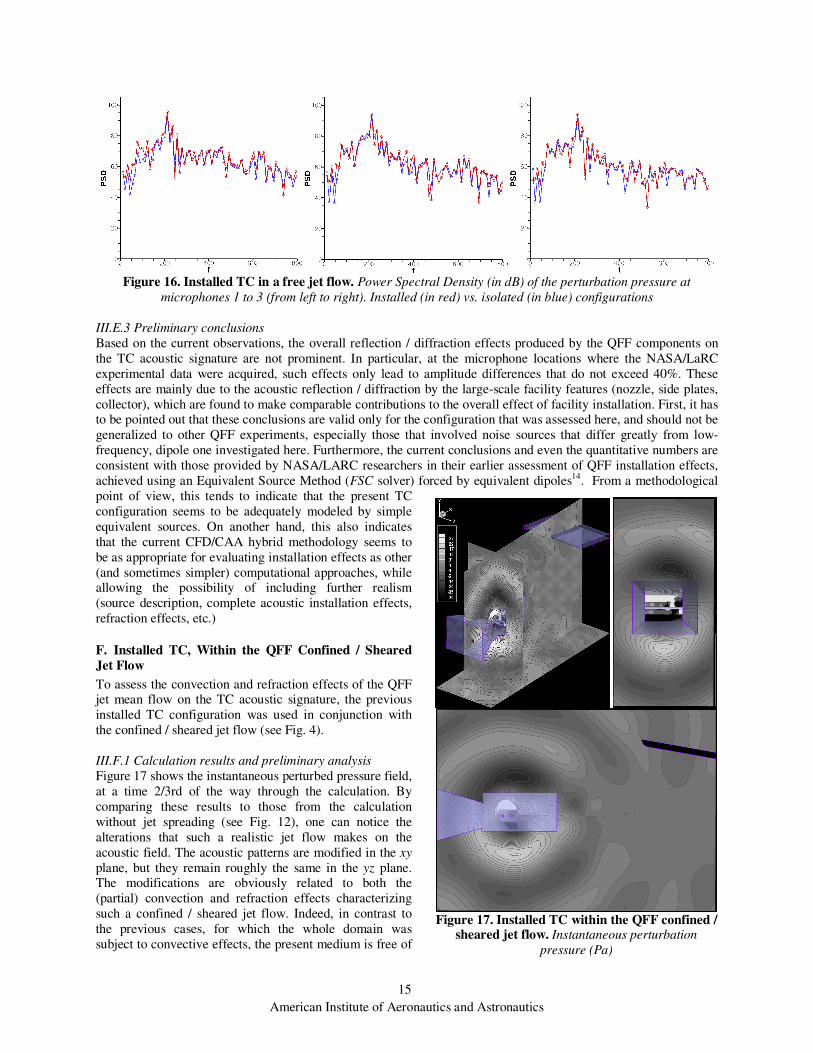
Figure 16 displays the PSD (Power Spectral Density) spectra associated with the time history signals of Fig. 15.

The trends previously observed in the time domain are also exhibited here, with all fully-installed TC spectra

matching the isolated case very closely, not only in terms of amplitude, but also in terms of shape.


15

Figure 16. Installed TC in a free jet flow. Power Spectral Density (in dB) of the perturbation pressure at

microphones 1 to 3 (from left to right). Installed (in red) vs. isolated (in blue) configurations

III.E.3 Preliminary conclusions

Based on the current observations, the overall reflection / diffraction effects produced by the QFF components on

the TC acoustic signature are not prominent. In particular, at the microphone locations where the NASA/LaRC

experimental data were acquired, such effects only lead to amplitude differences that do not exceed 40%. These

effects are mainly due to the acoustic reflection / diffraction by the large-scale facility features (nozzle, side plates,

collector), which are found to make comparable contributions to the overall effect of facility installation. First, it has to be pointed out that these conclusions are valid only for the configuration that was assessed here, and should not be

generalized to other QFF experiments, especially those that involved noise sources that differ greatly from low-

frequency, dipole one investigated here. Furthermore, the current conclusions and even the quantitative numbers are

consistent with those provided by NASA/LARC researchers in their earlier assessment of QFF installation effects,

achieved using an Equivalent Source Method (FSC solver) forced by equivalent dipoles14. From a methodological

point of view, this tends to indicate that the present TC

configuration seems to be adequately modeled by simple

equivalent sources. On another hand, this also indicates

that the current CFD/CAA hybrid methodology seems to

be as appropriate for evaluating installation effects as other

(and sometimes simpler) computational approaches, while allowing the possibility of including further realism

(source description, complete acoustic installation effects,

refraction effects, etc.)

F. Installed TC, Within the QFF Confined / Sheared Jet Flow

To assess the convection and refraction effects of the QFF jet mean flow on the TC acoustic signature, the previous

installed TC configuration was used in conjunction with

the confined / sheared jet flow (see Fig. 4).

III.F.1 Calculation results and preliminary analysis

Figure 17 shows the instantaneous perturbed pressure field,

at a time 2/3rd of the way through the calculation. By

comparing these results to those from the calculation

without jet spreading (see Fig. 12), one can notice the

alterations that such a realistic jet flow makes on the

acoustic field. The acoustic patterns are modified in the xy

plane, but they remain roughly the same in the yz plane. The modifications are obviously related to both the

(partial) convection and refraction effects characterizing

such a confined / sheared jet flow. Indeed, in contrast to

the previous cases, for which the whole domain was

subject to convective effects, the present medium is free of

Figure 17. Installed TC within the QFF confined /

sheared jet flow. Instantaneous perturbation

pressure (Pa)


16

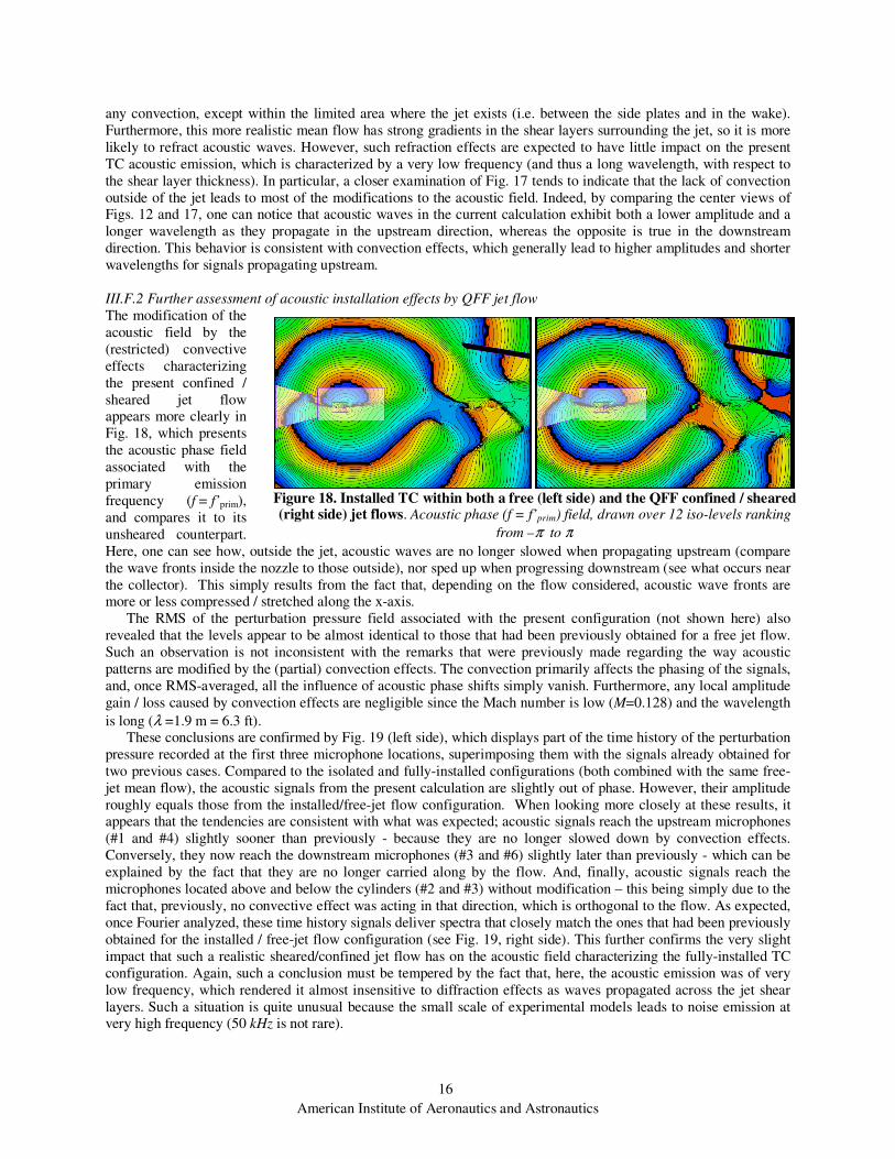
Figure 18. Installed TC within both a free (left side) and the QFF confined / sheared (right side) jet flows. Acoustic phase (f = f’prim) field, drawn over 12 iso-levels ranking

from –π to π

any convection, except within the limited area where the jet exists (i.e. between the side plates and in the wake).

Furthermore, this more realistic mean flow has strong gradients in the shear layers surrounding the jet, so it is more

likely to refract acoustic waves. However, such refraction effects are expected to have little impact on the present

TC acoustic emission, which is characterized by a very low frequency (and thus a long wavelength, with respect to

the shear layer thickness). In particular, a closer examination of Fig. 17 tends to indicate that the lack of convection

outside of the jet leads to most of the modifications to the acoustic field. Indeed, by comparing the center views of Figs. 12 and 17, one can notice that acoustic waves in the current calculation exhibit both a lower amplitude and a

longer wavelength as they propagate in the upstream direction, whereas the opposite is true in the downstream

direction. This behavior is consistent with convection effects, which generally lead to higher amplitudes and shorter

wavelengths for signals propagating upstream.

III.F.2 Further assessment of acoustic installation effects by QFF jet flow

The modification of the

acoustic field by the

(restricted) convective

effects characterizing

the present confined /

sheared jet flow appears more clearly in

Fig. 18, which presents

the acoustic phase field

associated with the

primary emission

frequency (f = f’prim),

and compares it to its

unsheared counterpart.

Here, one can see how, outside the jet, acoustic waves are no longer slowed when propagating upstream (compare

the wave fronts inside the nozzle to those outside), nor sped up when progressing downstream (see what occurs near

the collector). This simply results from the fact that, depending on the flow considered, acoustic wave fronts are more or less compressed / stretched along the x-axis.

The RMS of the perturbation pressure field associated with the present configuration (not shown here) also

revealed that the levels appear to be almost identical to those that had been previously obtained for a free jet flow.

Such an observation is not inconsistent with the remarks that were previously made regarding the way acoustic

patterns are modified by the (partial) convection effects. The convection primarily affects the phasing of the signals,

and, once RMS-averaged, all the influence of acoustic phase shifts simply vanish. Furthermore, any local amplitude

gain / loss caused by convection effects are negligible since the Mach number is low (M=0.128) and the wavelength

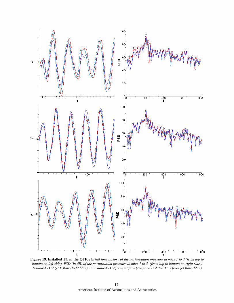
is long (λ =1.9 m = 6.3 ft). These conclusions are confirmed by Fig. 19 (left side), which displays part of the time history of the perturbation

pressure recorded at the first three microphone locations, superimposing them with the signals already obtained for

two previous cases. Compared to the isolated and fully-installed configurations (both combined with the same free-

jet mean flow), the acoustic signals from the present calculation are slightly out of phase. However, their amplitude

roughly equals those from the installed/free-jet flow configuration. When looking more closely at these results, it appears that the tendencies are consistent with what was expected; acoustic signals reach the upstream microphones

(#1 and #4) slightly sooner than previously - because they are no longer slowed down by convection effects.

Conversely, they now reach the downstream microphones (#3 and #6) slightly later than previously - which can be

explained by the fact that they are no longer carried along by the flow. And, finally, acoustic signals reach the

microphones located above and below the cylinders (#2 and #3) without modification – this being simply due to the

fact that, previously, no convective effect was acting in that direction, which is orthogonal to the flow. As expected,

once Fourier analyzed, these time history signals deliver spectra that closely match the ones that had been previously

obtained for the installed / free-jet flow configuration (see Fig. 19, right side). This further confirms the very slight

impact that such a realistic sheared/confined jet flow has on the acoustic field characterizing the fully-installed TC

configuration. Again, such a conclusion must be tempered by the fact that, here, the acoustic emission was of very

low frequency, which rendered it almost insensitive to diffraction effects as waves propagated across the jet shear

layers. Such a situation is quite unusual because the small scale of experimental models leads to noise emission at very high frequency (50 kHz is not rare).


17

Figure 19. Installed TC in the QFF. Partial time history of the perturbation pressure at mics 1 to 3 (from top to

bottom on left side). PSD (in dB) of the perturbation pressure at mics 1 to 3 (from top to bottom on right side).

Installed TC / QFF flow (light blue) vs. installed TC / free- jet flow (red) and isolated TC / free- jet flow (blue)


18

Conclusions and Perspectives

The present study described a numerical investigation of the acoustic installation effects related to the Tandem

Cylinder aeroacoustic experiments in the NASA/LaRC QFF facility. The numerical computations were conducted

using a hybrid approach involving a weak coupling between the nearfield CFD computation and the CAA

calculation aimed at propagating the nearfield information to the far field. The computations employed the so-called

‘surface’ coupling approach, which was recently improved to better handle acoustic backscattering that is typical of

airframe configurations installed within a wind tunnel facility. Several CFD/CAA coupled calculations of the TC

configuration were conducted, all of which involved the combination of 1) a common CFD stage that utilized

previously obtained numerical solutions, and 2) various CAA stages focused on different aspects of the installation

effects. Specifically, the latter allowed numerical evaluations of the effect of each component (e.g., nozzle, collector, etc.) or a feature characterizing the NASA/LaRC QFF facility (e.g., confined jet vs. co-flow). The impact

of each installation effect on the acoustic signature of the TC configuration was assessed. The primary conclusion

from these computations is that the total magnitude of the installation effects associated with the TC model in the

QFF is rather modest. In particular, at the 6 microphone locations used during testing, the installation effects are

expected to account for amplitude differences of less than 40% in magnitude (with the change in amplitude varying

between –1.35 dB and +3.45 dB, depending on the microphone location). Most of these effects are due to the QFF

components themselves, resulting either from the confinement of the acoustic emission by side plates, or from

additional reflection / diffraction of radiated waves by both the collector plate and the nozzle. Very slight

modifications are due to the QFF jet flow, which mainly results from convection being restricted to the region of the

jet. From a methodological point of view, the present results contribute to a more meaningful comparison between

QFF acoustic data and noise predictions based on the free-field TC configuration. Such results are thus an important step in employing the QFF measurements in semi-empirical prediction techniques for landing gear noise, such as

that proposed by Lopes et al.20. Furthermore, these results also provide an additional validation / application of the

CFD/CAA surface coupling, and pave the way for more systematic utilization of such techniques for solving more

complex problems involving significant acoustic installation effects, for which commonly used computational

approaches (such a CFD/FWH one) are not applicable21.

Obviously, the conclusions drawn in this study are valid only for the configuration that was assessed here, and

should not be generalized to other QFF experiments, especially those involving noise sources that differ greatly from

the low-frequency, dipole dominating the noise radiation associated with the TC configuration. In particular,

considering the relatively high frequencies characterizing usual airframe noise sources, most QFF acoustic

experiments should be more strongly influenced by the diffraction across the shear layers surrounding the QFF jet

flow. For this reason, follow-on computations are planned to extend the present results to include high frequency sources such as simple distributions of acoustic monopoles and dipoles to provide a more complete numerical

assessment of the diffraction effects associated with the spreading of the QFF jet. Several jet flow speeds and

spreading angles will be studied, including a wide range of frequencies. This will provide an opportunity to check

the validity of the infinitely thin shear layer correction that is commonly applied to QFF experimental data. The

outcome of this prospective study will help assess further acoustic installation effects that may be important in the

type of testing typically done in the NASA/LARC QFF facility.

Acknowledgments

The present work was funded by ONERA and conducted while the first author was in residence at NASA Langley

Research Center as part of a NASA-ONERA collaboration related to airframe noise. The authors would like to thank

Dr. Florence Hutcheson and Mr. Daniel Stead for the detailed information regarding the QFF experiment. The

authors would also like to acknowledge Dr. Ana Tinetti, whose past work and informal exchanges helped guide the

present study.

References 1Polacsek, C., Burguburu, S., Redonnet, S. and Terracol, M., “Numerical Simulations of Fan Interaction Noise using a

Hybrid Approach,” AIAA Journal, Vol. 44, No. 6, June 2006. 2Ffowcs Williams, J. E. and Hawkings, D. L., “Sound Generation by Turbulence and Surfaces in Arbitrary Motion,”

Philosophical Transactions of the Royal Society of London A, Vol. 342, 1969, pp. 264–321. 3Redonnet, S., “On the Numerical Prediction of Aerodynamic Noise via a Hybrid Approach - Part 1: CFD/CAA Surfacic

Coupling Methodology, Revisited for the Prediction of Installed Airframe Noise Problem,” AIAA Paper 2010-3709, 16th AIAA/CEAS Aeroacoustics Conference, Stockholm, Sweden, June 2010.

4Redonnet, S., “Simulation de la Propagation Acoustique en Présence d’écoulements Quelconques et de Structures Solides, par Résolution Numérique des équations d’Euler,” PhD Thesis, Université Bordeaux I, 2001.


19

5Manoha, E., Herrero, C., Sagaut, P. and Redonnet, S., “Numerical Prediction of Airfoil Aerodynamic Noise,” AIAA Paper 2002-2573, 8th CEAS/AIAA Aeroacoustics Conference, Breckenridge, USA, June 2002.

6Guenanff, R., “Couplage Instationnaire Navier-Stokes/Euler pour la Génération et le Rayonnement des Sources de Bruit Aérodynamique,” PhD Thesis, Rennes University, 2004, No. 3138.

7Terracol, M., Manoha, E., Herrero, C., Labourasse, E., Redonnet, S. and Sagaut, P., “Hybrid Methods for Airframe Noise

Numerical Prediction,” Theoretical and Computational Fluid Dynamics, Vol. 19, No.3, July 2005. 8Jenkins, L. N., Khorrami, M. R., Choudhari, M. M. and McGinley, C. B., “Characterization of Unsteady Flow Structures

Around Tandem Cylinders for Component Interaction Studies in Airframe Noise,” AIAA Paper 2005-2812, 11th AIAA/CEAS Aeroacoustics Conference, Monterey, USA, May 23-25, 2005.

9Jenkins, L. N., Neuhart, D. H., McGinley, C. B., Choudhari, M. M. and Khorrami, M. R., “Measurements of Unsteady Wake Interference Between Tandem Cylinders,” AIAA Paper 2006-3202, 36th AIAA Fluid Dynamics Conference and Exhibit, San Francisco, USA, June 5-8, 2006.

10Hutcheson, F. V. and Brooks, T. F., “Noise Radiation from Single and Multiple Rod Configurations,” AIAA Paper 2006-

2629, 12th AIAA/CEAS Aeroacoustics Conference, Cambridge, USA, May 2006. 11Neuhart, D. H., Jenkins, L. N., Choudhari, M. M. and Khorrami, M. R., “Measurements of the Flowfield Interaction

Between Tandem Cylinders,” AIAA Paper 2009-3275, 15th AIAA/CEAS Aeroacoustics Conference, Miami, USA, May 2009. 12Lockard, D. P., Khorrami, M. R., Choudhari, M. M., Hutcheson, F. V. and Brooks, T. F., “Tandem Cylinder Noise

Prediction,” AIAA Paper 2007-3450, 13th AIAA/CEAS Aeroacoustics Conference, Roma, Italy, May 2007. 13Lockard, D. P., Choudhari, M. M., Khorrami, M. R., Neuhart, D. H., Hutcheson, F. V. and Brooks, T. F., “Aeroacosutic

Simulations of Tandem Cylinders with Subcritical Spacing,” AIAA Paper 2008-2862, 14th AIAA/CEAS AeroAcoustics Conference, Vancouver, Canada, May 2008.

14Tinetti, A. F. and Dunn, M. H., “Acoustic Simulations of an Installed Tandem Cylinder Configuration,” AIAA Paper 2009-

3158, 15th AIAA/CEAS AeroAcoustics Conference, Miami, USA, May 2009. 15Dunn, M. H. and Tinetti, A. F., “Aeroacoustic Scattering Via the Equivalent Source Method,” AIAA Paper 2004-2937, 10th

AIAA/CEAS Aeroacoustics Conference, Manchester, United Kingdom, May 2004. 16Redonnet, S., Manoha, E. and Sagaut, P. “Numerical Simulation of Propagation of Small Perturbations Interacting with

Flows and Solid Bodies,” AIAA Paper 2001-2223, 7th CEAS/AIAA Aeroacoustics Conference, Maastricht, The Netherlands, May 2001.

17Redonnet, S., Desquesnes, G. and Manoha, E., “Numerical Study of Acoustic Installation Effects with a Computational

Aeroacoustics Method”, AIAA Journal, Vol. 48, No. 5, May 2010. 18Redonnet, S., Mincu, C., Manoha, E., Caruelle, B. and Sengissen, A., “Computational Aeroacoustics of a Realistic Co-

Axial Engine in Subsonic and Supersonic Take-Off Conditions,” AIAA Paper 2009-3240, 15th AIAA / CEAS Aeroacoustics Conference, Miami, USA, May 2009.

19Cunha, G. and Redonnet, S., “An Innovative Interpolation Technique for Aeroacoustic Hybrid Methods,” to be presented at the 17th AIAA/CEAS Aeroacoustics Conference, Portland, Oregon, USA, June 2011.

20Lopes, L., Brentner, K. and Morris, P., “Framework for a Landing-Gear Model and Acoustic Prediction,” Journal of

Aircraft, Vol. 47, No. 3, 2010, pp. 763-774. 21Brès, G., Wessels, M. and Noelting, S., “Tandem Cylinder Noise Predictions Using Lattice Boltzmann and Ffowcs

Williams–Hawkings Methods,” AIAA Paper 2010-3791, 16th AIAA/CEAS Aeroacoustics Conference, Stockholm, Sweden, June 2010.

cfd-caa coupled calculations of a tandem cylinder ... · the cfd-caa coupling is based on cfd data...

Documents