cfd fire simulation in enclosures - ulisboa fire simulation in...validate it against the lnec...
TRANSCRIPT

CFD Fire Simulation in Enclosures
Application to Portela Airport (LIS)
Nelson Alexandre Pinto de Magalhães
Thesis to obtain the Masters Degree in
Aerospace Engineering
Jury
President: Professor Doutor Carlos Silvestre
Orienter: Professor Doutor José Carlos Pereira
Co-Orienter: Doutor Nelson Marques
Members: Professor Doutor Pedro Serrão
October 2007
Nelson A. Pinto de Magalhães
Doctor Nelson P. C. Marques
Professor José C. F. Pereira

2
Index
Abstract .................................................................................................................. 4
1. Introduction......................................................................................................... 5
1.1. Objective...................................................................................................... 5
1.2. Context ........................................................................................................ 5
1.3. Bibliographic Review.................................................................................... 6
1.4. Conclusions ............................................................................................... 11
2. Model Equations and Simulation Methodology................................................. 12
2.1. Simulation Process – STAR-CD ................................................................ 12
2.2. Fluid Flow model equations ....................................................................... 13
2.2.1. Navier-Stokes Equations..................................................................... 13
2.2.2. Reynolds Average Navier Stokes - ε−k Model.................................. 14
2.2.3. Buoyancy ............................................................................................ 17
2.3. Physical mechanisms ................................................................................ 17
2.3.1. Heat Source ........................................................................................ 17
2.3.2. Mass Source ....................................................................................... 17
2.3.3. Soot and Scalar Sources..................................................................... 18
2.3.3. Radiation ............................................................................................. 19
2.3.4. Visibility ............................................................................................... 24
2.4. Conclusions ............................................................................................... 25
3. Validation – LNEC case.................................................................................... 27
3.1. Adimensional Numbers.............................................................................. 29
3.2. Solid Modelling .......................................................................................... 31
3.3. Mesh Generation ....................................................................................... 31
3.4. Computational Domain Size and Boundary Conditions ............................. 32
3.4.1. Boundary Conditions ........................................................................... 34
3.4.2. Domain Size and Discretization Methods............................................ 36
3.4.3. Type of Boundary Conditions .............................................................. 39
3.5. Physical Modelling ..................................................................................... 41
3.5.1. Enthalpy and Fluid Sources inside the structure ................................. 41
3.5.2. Radiation ............................................................................................. 45
3.5.3. Wall Treatment.................................................................................... 47
3.6. Mesh Studies ............................................................................................. 50
3.7. Results....................................................................................................... 51

3
3.8. Conclusions ............................................................................................... 54
4. Airport Case ..................................................................................................... 56
4.1 Characterization.......................................................................................... 56
4.2. Solid Modelling .......................................................................................... 57
4.3. Mesh Generation ....................................................................................... 57
4.4. Boundary Conditions.................................................................................. 58
4.5. Heat Source............................................................................................... 62
4.6. Numerical Aspects ..................................................................................... 63
4.7. Results Analysis ........................................................................................ 67
4.8. Conclusions ............................................................................................... 70
Bibliography.......................................................................................................... 71

4
ABSTRACT
Fire in enclosures generates flow of hot air and smoke through the structure that
harbours it. This paper presents the development, validation and application of a
CFD methodology to simulate fire induced fluid flows in case of an indoor fire. The
CFD software STAR-CD was used to develop and test this methodology. The
computational model solves the steady-state Navier-Stokes equations using the
buoyancy extended ε−k model, while taking into account radiation and the
medium’s radiative properties. The influence of the computational domain and
associated boundary conditions was assessed. The overall CFD methodology was
validated against a comprehensive set of data obtained from experimental tests [4],
allowing detailed temperature and velocity comparisons. STAR results agree well
with the experiments having a temperature over-prediction mostly on the upper (hot)
layer of the flow. The methodology was applied to the simulation of a fire in an
idealized configuration of Lisbon’s Airport. The modelled situation presents little
potential harm but results show that it is possible to minimize risk of toxic gases
asphyxiation. It is outlined that CFD combined with optimization tools may drive
ventilation expert systems for smoke management in an indoor fire scenario.
ACKNOWLEDGEMENTS
The author would like to thank Doctor João Viegas, from LNEC, for sharing the
experimental results from his PhD thesis [4]. These measurements were essential to
the model validation.
Additionally, the author would also like to thank ANA Aeroportos de Portugal, S.A.
for accepting to be part this project. Namely, Mr. Ricardo Patela and Eng. José
Ramalhete should be recognized for their support and Mr. Gonçalo Pacheco, from
IST, for aiding in the CAD design of the airport.
On a more personal aspect, the author wishes to thank his supervisor, Professor
José Carlos Pereira, for his excellent contributions, and his coordinator, Doctor
Nelson Marques, for his support and dedication. His clear vision of the goal and
structured analysis made this project and model all it could be.

5
1. INTRODUCTION
1.1. Objective
To develop a Computational Fluid Dynamics (CFD) simulation methodology suited
to the study of fire driven flows. Validate it against the LNEC experimental case
measurements. Apply this methodology to a fire occurrence in the boarding terminal
of Lisbon’s airport, analyze the results and draw relevant conclusions.
1.2. Context
The occurrence of a fire in a building enclosure can lead to serious losses of both
lives as well as property (estimated at around 1% of the world’s GDP [10]). In the
past years this was not seen as a priority but recently a lot of emphasis has been
given to safety issues in buildings. With recent events this has become a major
concern for public safety authorities as well, leading to a revisal of civil protection
authority’s powers and duties [9].
Clever designing and planning is highly encouraged as buildings become
increasingly complex in geometry, making fire and smoke behaviour very difficult if
not impossible to predict. Henceforth, correlation-based methods such as zone
models ([3]) were used to aid the designer/safety technician to assess this behaviour.
Today, given the sophistication of current CFD codes and the computational power of
commonly available personal workstations, a trend is emerging whereby the global
fire flow pattern is simulated. This increase on the complexity of the physical
modelling, on the other hand, demands careful implementation because several
physical phenomena are at play, from combustion to radiative heat transfer, from
buoyancy to turbulence. Success in the application of these techniques depends on
the understanding of the interplay between all these physical processes and the
range of fundamental studies that try to match this interplay versus accurate
experimental data.
The current work tackles this very difficult problem by doing a synthesis of best-
practice approaches to model fire flow features, validating it against available
experimental data and, finally, studying a fire situation on Lisbon’s airport.

6
1.3. Bibliographic Review
A bibliographic review across available literature has shown that there has been a
convergence of conclusions towards common methodologies. Various CFD codes
have been used and applied to different situations. Table 1 to Table 4 organize these
findings.
The study which has the biggest amount of interest to us is the one performed in
terminal 2 of Munich Airport [13].
In most of these references, the authors perform transient studies [13], [14], [15]
even when they are after the steady state condition. The physical phenomena itself is
highly unstable due to the strong coupling between density, temperature and
momentum.
Spatial resolution tends to be around 20 cm but study [13] performed in an airport,
employs resolution of 7 cm with 13 million cells. Time resolution varies from 0,01s
[21] to 1s [14] but is generally above 0,1s.
The turbulence model choice seems to have a concordance between studies.
When mentioned, a buoyancy modified variant of the k-ε model is always used. On
the other hand, radiation is both ignored [14] and [19] and firmly stated to be of the
utmost importance [16]. The models used range from discrete ordinates [16] to
discrete transfer models [15], [18] and [21].
Most literature suggests that to model fire in large enclosures one is not required
to model combustion in detail [18], but that fire power and sometimes mass sources
suffice [20]. For buoyancy usually two options are considered: ideal gas [13] and the
Boussinesq approach [14].
The set of studied parameters are the temperature profiles [13] to [21], the smoke
distribution [13], [14], [16], [19] and [21] and the species concentrations [21]. Each
work validates its solutions against experimental scenarios and/or simulations.
A summary of the studies mentioned here is represented from Table 1 to Table 4.
More general reviews of these matters can be found in [11], who provides a review
of the scientific work on fire research up until that time, or in [12], where the author
has accomplished to update the former work in the field of buoyancy dominated fire
flows.

Ref
#
13
14
15
16
17
Title Year Type of Simulation Software
Turbulence
model
Radiation
Model Buoyancy Fire Modellation
GTD GmbH - Simulation of
Smoke Distribution and
Extraction in Terminal 2 of
Munich Airport 2005
Fire in Terminal 2 at Munich
Airport FLUENT n/a n/a Ideal Gas
velocity inlet and
volumetric model
HSL - Evaluation of CFD to
predict smoke movement in
complex enclosed spaces 2004
1-Underground station
2-Offshore accommodation module
3-Building under construction CFX
buoyancy
modified k-ε vs
k-ε not used
Boussinesq
relation vs Ideal
Gas
Volumetric heat source
model (no combustion) Vs Eddy-break-up combustion
model
Comparison of a CFD Fire
Model against a Ventilated Fire
Experiment in an Enclosure 2004
Parallelepipedic room with
one opening CFX
buoyancy
modified k-ε and
SST discrete transfer n/a
Volumetric heat source
model (no combustion)
Fire and smoke distribution in
a two-room compartment
structure 2002 2-room compartment own code
buoyancy
modified k-ε
Discrete
Ordinates n/a Eddy-Break-up
Mott MacDonald - Modelling
Fire and Smoke Spread in
Enclosed Spaces 2001 Metro Tube fire n/a k-ε n/a Ideal Gas
inert model with design
HRR (fire growth in
space and time)
Table 1
Previous Studies in Enclosures Fires (1 of 4)

8
Ref
#
13
14
15
16
17
Title Year
Spatial
Resolution
Time
Resolution
[s]
Parameters
Studied
Type of
validation
GTD GmbH - Simulation of
Smoke Distribution and
Extraction in Terminal 2 of
Munich Airport 2005
6 - 13 M
dxyz=0,07m -
0,14m n/a
Smoke, flow
field,Temperature
Release of
smoke in the
Airport itself
HSL - Evaluation of CFD to
predict smoke movement in
complex enclosed spaces 2004 93 - 156 K 0,2 - 1,0
Smoke, flow
field,Temperature
Small scale in
phase 2
Comparison of a CFD Fire
Model against a Ventilated Fire
Experiment in an Enclosure 2004
200K with dxyz
from 0,002m to
0,3m 0,1 - 0,3
Flow field and
Temperature
Exactly as
modeled in
True Geometry
Fire and smoke distribution in
a two-room compartment
structure 2002
dx=0,056m
dy=0,14m
dz=0,34m n/a
Smoke (soot),
Temperature, Flow field,
and species mass
concentrations
Exactly as
modeled in
True Geometry
Mott MacDonald - Modelling
Fire and Smoke Spread in
Enclosed Spaces 2001 Ideal Gas
inert model with
design HRR (fire
growth in space
and time)
Smoke, flow
field,Temperature
Memorial
Tunnel Fire
Tests
Table 2 Previous Studies in Enclosures Fires (2 of 4)

9
Ref
#
18
19
20
21
Title Year Type of Simulation Software
Turbulence
model
Radiation
Model Buoyancy Fire Modellation
Fire Safety Engineering Group -
Fire Modelling
Standars/Benchmark 2001 Steckler room SMartFire
buoyancy
modified k-ε multi-ray
Boussinesq
relation vs Ideal
Gas
heat source(small fire)
vs combustion model
(Large fire)
HBI Haerter AG - CFD study of
Temperature and Smoke Distribution
in a Railway Tunnel with Natural
Ventilation System >2000 Railway Tunnel Fire FLUENT k-ε not used Ideal Gas
30 MW constant and 43
Kg/s at 1000K with 4,2%
of smoke
Pittsburgh Research
Laboratory - CFD Modelling of
Smoke Reversal >1999 Large channel CFD2000 k-ε n/a Ideal Gas
empirical smoke mass
flow rates
CESARE - Application of Field Model
and Two-zone Model to Flashover
Fires in a Full-scale Multi-room Single
Level Building 1997 Office building floor 16m*7m
CESARE-CFD
vs CFAST
buoyancy
modified k-ε discrete beams
taken into
account but
unspecified mixture fraction
Table 3 - Previous Studies in Enclosures Fires (3 of 4)

10
Ref
#
18
19
20
21
Title Year
Spatial
Resolution
Time
Resolution
[s]
Parameters
Studied
Type of
validation
Fire Safety Engineering Group -
Fire Modelling
Standars/Benchmark 2001
dx=0,06m
dy=0,065m
dz=0,06m 1,0 Temperature only
Steckler fire
case
HBI Haerter AG - CFD study of
Temperature and Smoke Distribution
in a Railway Tunnel with Natural
Ventilation System >2000 n/a 1,0
Smoke, flow
field,Temperature not performed
Pittsburgh Research
Laboratory - CFD Modelling of
Smoke Reversal >1999
dx=0,59m
dy=0,19m
dz=0,09m n/a
Flow field and
Temperature
fire tunnel by
Hwang and
Wargo
CESARE - Application of Field Model
and Two-zone Model to Flashover
Fires in a Full-scale Multi-room Single
Level Building 1997
dx=0,4m
dy=0,2m
dz=0,16m 0,01
Temp, Smoke, 02, C02
and CO
Exactly as
modeled in
True Geometry
Table 4 - Previous Studies in Enclosures Fires (4 of 4)

1.4. Conclusions
Underlying fire in enclosures we have physical phenomena which are often
naturally unstable. Even so, CFD simulations are quite common as an analysis tool in
these circumstances in spite of a lack of consensus regarding which combination of
models produces the best results.
These simulations require a large amount of CPU time and so, only more recently
have they been performed on larger buildings with more complex models.
Also, from the experimental validations observed, it is normal to have temperature
over-predictions in the order of 10-30%.

12
2. MODEL EQUATIONS AND SIMULATION METHODOLOGY
As stated in the first chapter, we aim to develop a simulation procedure whereby a
3D, heat-fluid flow coupled fire problem can be studied. Since the work has been
done using the STAR-CD tool-set, its framework is presented first, in section 2.1.
Afterwards, in section 2.2, we present the model equations for the different transport
processes, whereas section 2.3 contains a description of the modelling approach to
the other physical mechanisms that have been considered.
2.1. Simulation Process – STAR-CD
A CFD simulation commonly comprises the steps presented on Table 5, which
also details the tool we employed on each one of them.
Phase Software
Solid Modelling CAD (STAR-Design,
SolidWorks, etc.)
Surface Discretization pro-surf
Mesh Generation pro-am
Selection of the relevant physical
phenomena (Physical Modelling) pro-STAR
Boundary Conditions and Aero-
Thermodynamic properties of the
flow
pro-STAR
Flow Simulation STAR
Post processing pro-STAR
Table 5 CFD simulation phases
STAR-Design, pro-surf, pro-am, pro-STAR and Star all belong to the STAR-CD
suite software.

13
Examples for each of these steps will be shown later, when the test-cases
description is given, or in some of the appendices.
One feature of the STAR-CD tool-set is that, if the range of physical models
available by default is not sufficient to cover the user's needs, then one can program
his own, with Fortran, and can thus easily extend the range of applicability of STAR-
CD. This feature has been used in this work, as shown in later chapters. Most
notably, on appendixes 1 to 5, we provide the Fortran user coding for all the physical
models that were not available in STAR-CD and had to be included (i.e., coded) by
hand.
2.2. Fluid Flow model equations
2.2.1. Navier-Stokes Equations
In this section the model equations are shown as existing in [7], whose deductions
can be found both in [8] or [9].
The equations that express mass and momentum conservation in the fluid flow
stream, the Navier-Stokes equations, are expressed in ( 1 ) and ( 2 ) in their tensorial
form.
( )mj
i
suxt
=∂
∂+
∂
∂ρ
ρ ( 1 )
( ) ( )i
i
ijj
j
i sx
pu
xt
u+
∂
∂−=−
∂
∂+
∂
∂τρ
ρ ( 2 )
Where t stands for time; ix the Cartesian coordinates ( i = 1, 2, 3); iu is the
velocity component in the ix direction; p represents the static pressure; ρ the
density; ijτ the components of the stress tensor; ms the mass sources and is the
momentum sources. In this case is is equal to igρ− , where ig is the gravity
acceleration component in the ix direction.

14
2.2.2. Reynolds Average Navier Stokes - ε−k Model
To solve turbulent flow problems one approach consists in averaging ( 1 ) and ( 2 )
in time (RANS–Reynolds Average Navier-Stokes), turning ijτ into ( 3 ).
''3
22 jiij
k
k
ijij uux
us ρδµµτ −
∂
∂−= ( 3 )
Where µ represents the dynamic viscosity; ijδ the Kronecker delta, the dash
above indicates a time average; the )(' fluctuations in time and ijs the deformation
rate tensor. This tensor is given by ( 4 ).
∂
∂+
∂
∂=
i
j
j
i
ijx
u
x
us
2
1 ( 4 )
The effect of turbulence on the flow field (term '' ji uuρ− ) is modelled via additional
stresses. These are called Reynolds Turbulent Stresses.
For compressible flows an extra relation is necessary. This relation is the ideal gas
equation ( 5 ).
TM
R
p=ρ ( 5 )
Where R is the ideal gas constant and M is the molar mass of the gas.
Finally, to close the RANS equation system, a model for the turbulent Reynolds
Stresses is assumed such as similarly to laminar flow, we have:
ij
k
ktijtji k
x
usuu δρµµρ
+
∂
∂−=−
3
2'' ( 6 )
In which tµ is the turbulent viscosity. This parameter is a function of the flow field,
not the fluid, and k is, by definition, the turbulent kinetic energy ( 7 ). Prandtl [22]

15
suggested a functional relation with velocity and length scales typical of a turbulent
field. In the ε−k model the scales are k for velocity and ε the dissipation rate of
k for length. Thus the Prandtl’s functional relation is stated in ( 8 ).
''5,0 ii uuk = ( 7 )
ε
ρµ
µ
µ
kCft = ( 8 )
Where µC is an empirical coefficient often considered constant and µf is a
function that depends on the different variants of the model.
Equations ( 9 ) and ( 10 ) state the transport equations for k and ε .
( )
( )NLt
i
i
i
i
tBt
jk
t
j
j
Px
uk
x
uPP
x
kku
xt
k
µρµερµ
σ
µµρ
ρ
+∂
∂
+
∂
∂−−+=
=
∂
∂
+−
∂
∂+
∂
∂
3
2 ( 9 )
( )
NLt
i
i
Bt
i
i
i
i
ttl
j
t
j
j
Pk
Cx
uC
kCP
kC
x
uk
x
uP
kC
xu
xt
µε
ερε
ρµε
ρµµεε
σ
µµερ
ερ
εεεε
ε
ε
14
2
23
3
2
+∂
∂+−+
+
∂
∂
+
∂
∂−=
∂
∂
+−
∂
∂+
∂
∂
( 10 )
With:
j
i
ijx
usP
∂
∂= ( 11 )
ith
i
Bx
pgP
∂
∂−=
ρσ
1
,
( 12 )
∂
∂
+
∂
∂−−
∂
∂−=
i
i
ti
i
j
i
ji
t
NLx
uk
x
uP
x
uuuP
µ
ρ
µ
ρ
3
2'' ( 13 )

16
In which σ represents the turbulent Prandtl’s numbers (ratio between kinetic and
thermal diffusivities) and Table 6 indicates the values of the several constants for the
standard model. In this model it is possible to obtain turbulent viscosity from ( 8 ) by
assuming µf equals to 1.
µC kσ εσ hσ mσ 1εC 2εC 3εC 4εC κ E
0,09 1,0 1,22 0,9 0,9 1,44 1,92 0/1,4* -0,33 0,419 9,0**
* 1,4 if PB > 0, otherwise Cε3 = 0.
** Only for flat walls
Table 6 Standard k-ε model constants
The total enthalpy (H) transport equation is given by ( 14 ).
( ) ( )hii
j
ijijhj
j
susx
puFHu
xt
H++
∂
∂−=−+
∂
∂+
∂
∂τρ
ρ, ( 14 )
With
huuH ii +=2
1 ( 15 )
000 HTcTch pp +−= ( 16 )
Where the diffusive energy flux jhF , is given by ( 17 ), hs are the energy sources, h
is the enthalpy, pc the specific heat at constant pressure and temperature T, 0
pc the
specific heat at constant pressure at reference temperature (293 K) and 0H the
formation enthalpy of the substance the fluid is made of (assumed just one
substance for writing simplicity).
'', hux
TkF j
j
jh ρ+∂
∂−= ( 17 )

17
Also due to turbulence a diffusive energy flux appears. This flux is associated with
the fluctuations of the enthalpy and velocities averaged field. In the turbulent viscosity
model these averaged quantities are obtained from ( 18 ).
jth
t
jx
hhu
∂
∂−=
,
''σ
µρ ( 18 )
2.2.3. Buoyancy
STAR-CD can accommodate any form of user-specified momentum source field,
but it contains built-in provision of body forces, arising from buoyancy. The relevant
expressions are stated in ( 19 ).
)( 0ρρ −= ii gs ( 19 )
Where ig is the gravitational acceleration component in direction ix and 0ρ is the
reference density.
2.3. Physical mechanisms
2.3.1. Heat Source
The fire effect is modelled via a heat-source term in the energy equation, to cater
for the combustion contribution to heat the air. The model used is a volumetric source
stated in ( 14 ) as hs . In our steady-state simulations the heat release rate from the
fire to the surrounding air is constant.
The inclusion of this model has required the coding of a routine in a file named
“sorent.f” presented in Appendix 1. This routine is employed by STAR to define a
source term for each cell.
2.3.2. Mass Source
The insertion of propane in the domain is modelled via mass source term in the
mass conservation equation as stated in ( 1 ). In this work air is the only fluid in the

18
domain. To compensate the fact that it is propane ( molgHCM 1,44)( 83 = ) and not air
( molgairM 9,28)( = ) which enters the domain, the propane flux is corrected
according to the following equation:
83)(
)( 83HCdomain m
airM
HCMm && = ( 20 )
This source was coded in subroutine “fluinj.f”, shown in Appendix 2.
2.3.3. Soot and Scalar Sources
Besides heat, fire usually produces soot, which is a mass of unburned fuel
residues. Its production usually takes the form of particulate matter, which is
airborne. We have considered [29] that relate soot fraction as a percentage of burnt
fuel. STAR allows the calculation of user defined scalars transported with the flow by
solving a transport equation for each scalar ( 21 ).
( ) ( )φφφ
φφ ∇∇+=∇+∂
∂Csu
t
r ( 21 )
Where φ is the transported scalar, ur
is the fluid velocity, φs is the source term and
φC is the diffusivity coefficient assumed constant in this work with default STAR-CD
values.
It is also possible for STAR-CD to fix the scalar concentrations in a prescribed
volume by using proper coding in an add-on subroutine, called “sorsca.f”. This
subroutine (shown in appendix 3) was used to model CO2 and H2O sources to
account for the medium radiative properties and the stoichiometry of the global
chemical reaction of propane ( 22 ).
)(2)(2)(2)(83 435 ggggOHCOOHC +→+ ( 22 )

19
The smoke particulates produced by a fire primarily consist of soot, and the
production of particulates can be estimated as follows:
fpp mym = ( 23 )
Where py is the particle yield and fm the mass of fuel burned.
Klote and Mike [29] offer a list of values of particle yield for a number of materials
from small-scale experiments of turbulent flaming combustion.
In appendix 3 we offer the user coding that was ran with STAR-CD in order to
model the scalar sources/sinks.
2.3.3. Radiation
When applicable, the radiative heat transfer is modelled with the Discreet
Ordinates (DO) method which is available in STAR-CD.
As a beam is traced through the medium, its radiant intensity I in the direction Ω is
absorbed and incremented by the intervening material according to the following
equation:
∫ ΩΩΩΩ+++−=π
π4
')'()',(4
)( dIpk
IkIkkds
dI sbasa ( 24 )
Where s is the distance in the direction Ω, bI the black body emissive power of
the material at temperature )( 4 πσTIT b = , ak the absorption coefficient, sk the
scattering coefficient and p is the probability that the radiation incident in direction Ω
will be scattered to within dΩ of Ω.
Thermal radiation within participating media is governed by the radiative transfer
equation (RTE) given by ( 24 ). Re-written in terms of radiant intensity for a specific
wavelength λ this becomes:

20
∫ ΩΩ+++−=π
λλ
λλλλλλ
π4
)(4
)( dIk
IkIkkds
dI sbasa ( 25 )
Where λI is the radiative intensity at wavelength λ , λak the absorption coefficient
at wavelength λ , λsk the scattering coefficient at wavelength λ , λbI the black body
intensity at wavelength λ and Ω the solid angle with:
)1(
225
1
−=
TCbe
CI
λλλ
( 26 )
Where C1 = 0,595522 x 10⁻¹⁶ W m2/s and C2 = 0,01439 m K.
When the absorption and scattering coefficients of the media are independent of
wavelength, the media is called grey. In that case, the RTE can be integrated over
wavelength (or, equivalently, wave number) to produce a wavelength-independent
equation.
The boundary condition applied to the RTE for diffusely emitting (with emissivity
wε ) and reflecting (with reflectivity wρ ) boundaries is, for each wavelength λ:
w
sn
jw
bw dsnsIIsI Ω++= ∫< )0'.(
.)'()(rr
rrλλλ
π
ρε ( 27 )
Here, n is the unit surface vector directed outwards and s the unit vector along the
distance coordinate leaving the wall.
The radiant heat flux in a particular direction rqr
is given by the integration of the
radiant intensity over all solid angles and over the wavelength spectrum:
∫ ∫∞
Ω=0 4
)()(π
λ λddssIrqr
r ( 28 )

21
The radiation solution is coupled to the fluid dynamic solution through the
divergence of the radiative heat flux. This term exchanges energy between the fluid
and the radiant energy field. Given the intensity field, the divergence of the heat flux
is computed as
∫ ∫∞
Ω−=∇
0 4
4)(. λππ
λλ ddIIrq br
r ( 29 )
The discrete ordinates method solves field equations for radiation intensity
associated with a fixed direction sr
, representing one discrete solid angle. A detailed
description of the method can be found in [23] and [24]. As a result of ( 25 ), the form
of these ordinate equations (for each wavelength band) is
∑=
+++−=∇no
i
jjs
baisaii Iwk
IkIkkIs14
)(.π
λλλλ
r ( 30 )
Where jw is the quadrature weight that depends on the chosen ordinates, λbI is
the black-body intensity in the wavelength band and no is the number of ordinates.
The transport equation for each ordinate direction is discretised and solved
independently, using the same discretization and iterative solution practices as for
the other transport equations. For this reason, global iterations are necessary to
include the isotropic in-scattering terms in the RTE and to compute wall boundary
conditions. The angularly discretised boundary conditions take the form:
w
no
sn
jjw
bwwi snIII ∑<
++=)0'.(
, .rr
rr
π
ρε λ ( 31 )
∑=
−=∇no
i
jjbr IwIq1
4. λπr
( 32 )
The reflection term represents summation over incoming (incident) ordinate
directions.

22
The radiation solution provides a source term to the fluid’s energy equation as
given by ( 29 ). The discretised form of this source term at any cell is
∑=
−=∇no
i
jjbr IwIq1
4. λπr
( 33 )
This method was applied using an angular discretization S4 which means 24
ordinates. This means that energy will also be transported in these directions.
According to [4] the walls were assumed to have a “grey” behaviour, i.e. the
emissive, scattering and reflective properties do not vary with λ and its coefficients,
where applicable, were set with the following values:
Concrete
Emissivity 0,95
Reflectivity 0,05
Transmissivity 0,00
Table 7 Radiative Properties for Concrete
The properties of air were set according to [32]. This method for estimating the
radiative properties of the species assumes no scattering ( 0=sk ) and varies
absorption with both pressure and the temperature of the gases as stated in ( 34 )
and ( 35 ).
∑=
=no
i
iiCOOHa appTk1
, 22),( ( 34 )
Where i represents the different species in the gas, ip is the partial pressure and
ia is given by:
∑=
=5
0
)/1000(j
j
ji Tca ( 35 )

23
The coefficients jc are specific for each species and are stated in Table 8.
Coefficients H2O CO2
C0 -0,23093 18,741
C1 -1,12390 -121,310
C2 9,41530 273,500
C3 -2,99880 -194,050
C4 0,51382 56,310
C5 -1,86840E-05 -5,8169
Table 8 Species Radiation Coefficients
The implementation of this method in STAR was done via a user subroutine
named “radpro.f”. This subroutine can be found in appendix 4.
Soot was considered to add radiation absorption as described in [1]. The method
assumes that the increase in radiation absorption varies with the soot concentration
and temperature as shown in ( 36 ).
( )( )200000048,014,1232),( −+= TmmTk psootpa ( 36 )
Where pm is the mass concentration of particulates.
Total radiation absorption is then stated in ( 37 ).
22 ,),(),( COOHasootpaa pTkmTkk += ( 37 )
The inclusion of soot contribution for radiation absorption of the medium was also
included in subroutine “radpro.f” and can be found in appendix 4.

24
2.3.4. Visibility
This section describes the Jin [25] method which was used to estimate visibility
through smoke.
Smoke particles and irritants can reduce visibility and, while loss of visibility is not
directly life threatening, it can prevent or delay escape and thus expose people to the
risk of being overtaken by fire. Visibility depends on many factors, including the
scattering and absorption coefficient of the smoke, size and colour of smoke
particles, density of smoke, and the eye irritant effect of smoke. Visibility also
depends on the illumination in the room, whether an exit sign is light-emitting or light-
reflecting, and whether the sign is back or front-lighted. An individual’s visual acuity
and mental state at the time of a fire emergency are other factors.
Most visibility measurements through smoke have relied on test subjects to
determine the distance at which an object is no longer visible. However, variations in
visual observation of up to 25 to 30 percent can occur with the same observer under
the same test conditions but at different times. A correlation between the visibility of
test subjects and the optical density of the smoke has been obtained in extensive
studies by Jin [25], [26], [27] and [28].
Based on those studies, the relationship between visibility and smoke obscuration
is given by the following expression:
pmm
KS
α= ( 38 )
Where S is the visibility [ft], K the proportionality constant and mα is the specific
extinction coefficient [ft2/lb].
The proportionality constant (K) is dependent on the colour of the smoke,
illumination of the object, intensity of background illumination and visual acuity of the
observer [29].
Table 9 provides values of the proportionality constant based on the research of
Jin.

25
Situation Proportionality Constant K
Illuminated Signs 8
Reflecting Signs 3
Building Components in Reflected Light 3
Table 9 Proportionality Constants for Visibility
The specific extinction coefficient mα depends on the size distribution and optical
properties of the smoke particles. Seader and Einhorn in [30] and Steiner [31]
obtained values for the specific extinction coefficient mα from pyrolysis of wood and
plastics, as well as from flaming combustion of these same materials. Table 10
provides values for mα .
Mode of Combustion Specific Extinction Coefficient mα [ft2/lb]
Smouldering Combustion 21.000
Flaming Combustion 37.000
Table 10 Specific Extinction Coefficient for Visibility
To estimate visibility in this work it was calculated the visibility of each cell
considering a situation of “Building Components in Reflected Light” and thus 3=K
and “Smouldering Combustion” with 000.21=mα meaning that the combustion is
considered flameless for the visibility calculation. This is not the same to say visibility
is known on all cells for that changes with the direction of the sight. Nevertheless one
can estimate from the pattern of visibility presented whether there is or not visibility in
a certain direction.
Appendix 5 has the source code that implements this model for our purposes.
2.4. Conclusions
The fluid flow model equations used are the Reynolds-averaged Navier-Stokes
equations with an extra momentum source term for buoyancy. This source term is

26
used to include the effect of gravity and include the effects from body forces that
arise within the domain.
The physical mechanisms, such as the fire heat release rate, act as sources and
sinks in the calculation. These are characterized by empirical coefficients obtained
from various references depending on which model is being used. Visibility is a post-
processed field that is calculated through soot concentration.

27
3. VALIDATION – LNEC CASE
This chapter intends to validate the method described in chapter 2. It incorporates
the steps described before and the study of the influence of the physical models
used. At first a simple simulation is performed, followed by the application of the
methodology to the case described in [4].
As an initial test a simple geometry was created to observe and understand the
kind of features that would be present in our type of problems. The geometry chosen
represents a room with a small window and a door as shown in Figure 1. Both these
are open and the door opens to the inside, which was modelled through a baffle in
the mesh. There is a slow flow of hot air coming from the ground.
Figure 1
Simple Geometry and Boundary Conditions
The thermophysical properties employed in the STAR-CD simulation are:
ρ = f(T,P) - Ideal Gas
µ = 1.81e-05 kg/m.s - Constant
Cp = 1006 J/Kg.K - Constant
k = 0.02637 W/m.K - Constant
K-ε High Reynolds Number Turbulence model
Temperature calculation: Static Enthalpy Conservation
Buoyancy
The next two figures present some of the results.

28
Figure 2
Velocity and Temperature fields in the plume (left), section window (middle) and section door (right)
Figure 3
Temperature Isosurfaces in Celsius: 30º and 190º (left), 150º (middle) and 90º and 220º (right)
The results, although simple, already show the general behaviour of hot air. It rises
very hot from the heat source spreading through the ceiling and cooling down. The
window works as an outlet of hot air and while the door behaves both as an outlet
and inlet with hot air leaving through the top and cold entering from the bottom and
circling the room in the floor.
In order to correctly develop and test the modelling approach it is necessary to
compare to a real experimental situation. The chosen case was tested by João
Viegas and it is described in his PhD thesis [4]. The facility where the test was
performed is described in section 3.2 and belongs to LNEC – Laboratório Nacional
de Engenharia Civil (Civil Engineering National Laboratory) in Lisbon and it typifies
the physics that we wish to model.
The structure consists in a room with a window and a skylight connecting outside
and a corridor with two small windows and a door. (See Figure 4) In the selected
case study only the window and skylight of the room were open and the fire source
was placed in the middle of the corridor burning propane. There was wind coming
from the north.

29
3.1. Adimensional Numbers
The relevant adimensional quantities related to buoyancy are the Grashof,
Reynolds, Prandtl and Rayleigh numbers. The values and combinations of these
numbers will characterize the problem. Equations ( 39 ) through to ( 42 ) show the
definition of these quantities.
2
23
µ
ρβ TLgGr
∆= ( 39 )
22Re∞
∆=
u
TLgGr β ( 40 )
µ
ρ Lu∞=Re ( 41 )
GrRa Pr*= ( 42 )
Where β is the volumetric expansion coefficient, L is the characteristic length
based on the distance between the maximum and minimum temperature boundaries
and ∆T is the temperature range within the solution domain.
In problems involving natural or free convection, redistribution of energy is mainly
due to the force of gravity acting on a fluid of non-uniform density and causing fluid
motion. In mixed (i.e. free and forced) convection, the importance of buoyancy forces
can be measured by the ratio of Grashof to Reynolds numbers.
Equation ( 40 ) represents the ratio between buoyancy and inertial forces, so if it
exceeds unity, it is reasonable to assume that the flow is dominated by buoyancy.
Alternatively, if the ratio is very small, buoyancy forces may be ignored.
In natural convection problems the strength of buoyancy-induced flow can be
measured by the Rayleigh number, which is the product of the Prandtl and Grashof
stated in ( 42 ).
Rayleigh numbers less than 108 usually indicate laminar flow, with onset of
turbulence occurring over the range 108 < Ra < 1010.
It is not unusual for buoyancy-driven flows with high Grashof number (i.e. Gr >
109) to be naturally unstable. In such cases, a converged steady-state solution
cannot be obtained and the user should opt for the transient approach.

30
The assumed air properties for this calculation are stated in Table 11 for the inside
and outside the house.
Inside min max Outside Units
T 293,15 1000 293,15 K
ρ 1,205 0,3482 1,205 Kg/(m^3)
µ 1,82E-05 4,24E-05 1,82E-05 N.s/(m^2)
Cp 1005 1141 1005 KJ/(Kg.K)
Pr 0,713 0,726 0,713
β (Ideal Gas) 0,003411 0,001 0,003411 K^(-1)
g 9,8067 9,8067 9,8067 m/(s^2)
L 1 1 2 m
u 2,5 2,5 2,5 m/s
∆T 100 K706,85 Table 11
Properties used for Adimensional Study
Regarding the interior and exterior of the house the results are stated in Table 12
and Table 13 respectively.
8
min 10*67,4=Gr 10
max 10*04,1=Gr
11,1Re min
2 =Gr 78,3Re max
2 =Gr
810*39,3=Ra 1010*38,7=Ra
Table 12 Adimensional numbers inside the house
07,1Re min
2 =Gr
Table 13 Grashof Reynolds ratio outside the house
These results tell that, inside the house, this problem may be naturally unstable
(Gr > 109), is definitely dominated by buoyancy forces (Gr/Re2 > 1) and is most likely
a turbulent, strong buoyant flow. Outside the house it is expected a small competition
between buoyancy and inertial forces at first but not much and just close to the flow
“outlets” of the house.

31
3.2. Solid Modelling
The computational model was treated in Star-Design. The blueprints are
presented in appendix 13. Although what is shown in Figure 4 are the walls, it is in
fact the air that is necessary to mesh. This can be considered like the negative of the
actual domain for easier visualization.
15m
6m
15m
6m
Figure 4
Star Design Views of LNEC Geometry
3.3. Mesh Generation
The mesh (Figure 5) was generated in Pro-Am with the help of Pro-Surf. The
standard cell size outside the structure grows from 30 cm width to 960 cm and inside
varies from 10 cm to 30 cm. The intent of this mesh is not to have the best results but
to test the consistency of the model in a real geometry without being too time
consuming so that the run with the refined geometry can be performed without major
problems.
In order to avoid having just pressure boundaries in the openings, for that does not
correspond to reality, the computational domain considered extends far from the

32
structure. This enables the possibility of modelling wind effects by considering inlet
and pressure boundaries. North was aligned with the y-axis to facilitate the inclusion
of the wind.
Figure 5 Mesh Views
3.4. Computational Domain Size and Boundary Conditions
This section describes the boundary conditions used, their complexity and types
as well as the domain size.
It is now necessary to know if the boundary conditions affect the domain too much.
The chosen domain was domain 4 (see Table 15) as depicted in Figure 6 with inlet
conditions all around and the domain “box” aligned with the wind and a pressure
boundary as the wind “outlet”. The discretization method used was MARS on
momentum variables and UD on the remaining variables.

33
Domain
Pressure Boundary Condition
Initial Mesh
Inlet Boundary Conditions
Figure 6 Chosen Domain (right) and Boundary Conditions (left)
The results inside the structure already reveal the basic physics of the process.
Figure 7 shows what is happening inside. Inside the corridor there is an inlet at 600ºC
with |v|=0,1 m/s upwards and 0,4Kg/m3 in order to approach, in a simplified manner,
this type of buoyancy dominated flow.

34
Structure and Outside domain view
Corridor Section of Fire Zone
Surface of iso-temperature at 15ºC
Surface of iso-temperature at 42ºC
Figure 7 Initial Results in House
3.4.1. Boundary Conditions
At first, the wind was just a constant inlet but, as seen in Figure 8, this is not valid
for it will generate problems due to the unrealism of the assumption and the
buoyancy model used. So, according to [33] the atmospheric boundary layer was
considered as:
71
00
=
h
huu ( 43 )
)0(*0065,00 zzTT −−= ( 44 )
)0(**0 zzgPP piezo −+= ρ ( 45 )

35
With:
PaP
KT
mKg
mz
mh
smu
piezo 2,98006
33,2860
/1924,10
2800
0,50
/5,20
3
=
=
=
=
=
=
ρ
Where 0u is the velocity in the wind direction, T is the temperature and P is the
static pressure. The known wind conditions from the tests are 0u at a height of 0h .
According to the International Standard Atmosphere [33] (ISA) the conditions at 0z
(height of the reference cell) are 0ρ , 0T and piezoP .
Domain view
Rear view (wind “outlet”)
Figure 8 Incorrect results from wind modelling
Also, the assumption of constant piezometric pressure is not true according to the
ISA. Assuming it would cause unreal high velocities close to the boundary (Figure 9).
What can be used is the mean pressure over the “outlet” boundary to be zero so that
although the pressure increases as z decreases the mean value will be null. This
atmospheric model implies also that the density is a function of both temperature and
pressure so the Boussinesq approach is no longer an option.

36
Domain view
Domain view
Figure 9 Results with Pressure mean off
3.4.2. Domain Size and Discretization Methods
Initially, 3 meshes were created from the same initial mesh so that the smaller
ones were just part of the bigger (see Table 14). The analysis was conducted to
evaluate the mean pressure and mass fluxes over the openings of the structure.
These are the window and skylight and the results are shown in Figure 10.
Domain A Domain B Domain C Domain D
Upwind 10,6 10,6 19 25,4
Downwind 10,6 31,8 120,5 196
Side 12,6 12,6 31,1 63,4
Height 11,4 16 35,1 103
All values adimensionalised by the building height 2,84m Table 14
Initial Domains
The two methods used are Upwind (UD) and Monotone Advection and
Reconstruction Scheme (MARS) as described in [7]. The latter one is second order
accurate while the former is first order accurate. This was done to test whether the
methods would present a significant difference and applied to both momentum and
temperature variables. The remaining ones were calculated with UD. The MARS
method should be able to reproduce reality better but the UD is less costly
computationally.

37
0,1
0,15
0,2
0,25
0,3
0,35
0,4
0,45
A B C D
Domain
Ma
ss
Flu
x [
Kg
/s]
Window UD
Skylight UD
Window MARS
Skylight MARS
Figure 10
Mass Fluxes over the Window and Skylight using UD and MARS
As we can see by the results, although the pressure has basically no difference for
both UD and MARS the mass flux can reach differences up to 50%. One should take
into account that the summation of all mass fluxes, accounting also with the inlet,
should reduce to zero. And the variation of dimension of the domain is also playing
an important role as the results change considerably with the increase of its
dimensions.
At this point a study was proven necessary to determine which are the necessary
domain dimensions so that the results are “practically” unaffected by the boundary
conditions. At first 4 meshes were generated from the same “big” mesh. It was
studied the importance of Length (L) x Height (H) as shown in Table 15.
Domain 1 Domain 2 Domain 3 Domain 4
L x H 2L x H L x 2H 2L x 2H
Upwind 10,6 19,0 10,6 19,0
Downwind 10,6 20,8 10,6 20,8
Side 10,4 10,4 10,4 10,4
Height 11,4 11,4 24,7 24,7
All values adimensionalised by the building height 2,84m Table 15
Domain Sizes (1 to 4)

38
The results of these domains are presented in the following table
UD MARS UD MARS UD MARS UD MARS
Domain 1 145388 145388 -0,4092 -0,3387 100712 100712 0,41579 0,35596
Domain 2 145388 145388 -0,2673 -0,1155 100712 100712 0,26695 0,1265
Domain 3 144763 144764 -0,3945 -0,3269 100279 100280 0,40078 0,34449
Domain 4 144763 144764 -0,3985 -0,341 100279 100280 0,40637 0,3538
Mass Flux (Kg/s)
1,44 0,998
888K Inlet
Window Skylight
Area
(m^2)
Pressure*Area (N) Mass Flux (Kg/s) Area
(m^2)
Pressure*Area (N)
Table 16 Skylight and Window results (domains 1 to 4)
Again the pressures do not differ between methods but vary with the height as it
was seen before. The mass fluxes are influenced by the increase of L. To study this
behaviour four more meshes were generated: two of them with a height of H, and the
other two with a height of 2H as Table 17 shows.
Domain 5 Domain 6 Domain 7 Domain 8
1.4L x H 3L x H 1.4L x 2H 3L x 2H
Upwind 14,2 25,4 14,2 25,4
Downwind 14,0 32,6 14,0 32,6
Side 10,4 10,4 10,4 10,4
Height 11,4 11,4 24,7 24,7
All values adimensionalised by the building height 2,84m Table 17
Domain Sizes (5 to 8)
The results obtained are presented in Figure 11 organized by discretization
scheme and growing length.

39
Parametric study Upwind (blue) and MARS (orange)
L x H
2L x H
3L x H1.4L x 2H
3L x 2H
L x H
2L x H
3L x 2H
1.4L x HL x 2H2L x 2H
1.4L x H
3L x H
L x 2H1.4L x 2H2L x 2H
0,000
0,090
0,180
0,270
0,360
0,450
144600 144800 145000 145200 145400 145600
Window Mean Pressure [Pa]
L(reference lenght) =10,6 [m], H(reference height)=11,4 [m]
Win
do
w M
ass F
lux [
kg
/s]
Figure 11
Parametric Study
The upwind scheme seems to be heavily influenced by the boundary locations,
maybe due to the nature of the phenomena. However, the MARS scheme, at H=25,
produces steady and feasible results. Therefore the chosen domain, to run the
calculations, was domain 4 (2Lx2H) using MARS discretization method only in the
momentum variables because the temperature solution tended to unrealistic results
in the closed part of the corridor.
3.4.3. Type of Boundary Conditions
A study of the type of BCs to be used in the side and top boundaries of the mesh
was also performed. The question resided in having one inlet boundary and pressure
all around (case 1) or one pressure boundary at the end and inlet all around (case 2)
as depicted in Figure 12.

40
Case 1 – Inlet BC
Case 1 – Pressure BCs
Case 1 – All BCs
Case 2 – Inlet BCs
Case 2 – Pressure BC
Case 2 – All BCs
Figure 12 Different Approaches for Boundary Conditions
The results of both calculations did not differ significantly but the model with the
inlet conditions all around proved itself more robust and faster in the computation.
The selection of the reference cell proved to be of extreme importance for the
buoyancy calculations. The values provided had to be in full accordance to what
should be expected to the penalty of instability and divergence of the calculation.
Even so, the nature of the phenomena itself is unstable as we have seen in
section 3.1 so the calculation must be done providing small changes in every run
until the problem is fully modelled.
The stabled and physically realistic solution is presented in Figure 13.
Additionally to this work, a study was also conducted to assess the external wind
influence on a fully developed indoor fire by Magalhães, Marques and Pereira in [36].
This paper was presented in October 2007 at the Advanced Research Workshop on
“Fire Computer Modeling” in Santander, Spain.

41
Velocity and Pressure fields
Pressure Sections
Figure 13 Feasible Wind Solution
3.5. Physical Modelling
This section will describe the process of physical modelling and increasing
complexity up till the satisfactory convergence of the CFD solution towards the
experimental results.
3.5.1. Enthalpy and Fluid Sources inside the structure
So far all the calculations had a simple hot inlet inside the structure. It was now
time to insert the correct heat power. From the experimental results, [ ]KWQc 3,173=&
and [ ]sgm propane 73,3=& . If the inlet option was used with this mass flux, enthalpy
equation would force a temperature of [ ]CTinlet º27061= . This approximation was
unacceptable for the temperature is too high. According to [3] the flame maximum
temperature should not exceed 2200 ºC.
To correct this problem a different approach was considered as in [13]. This time
an enthalpy source was used where the flame was and all meshes have the same
source (See Figure 14).

42
Figure 14
Enthalpy Source
The results obtained are presented in Figure 15.
Iso-Temperature Surfaces
Temperature and Velocity Fields
Figure 15 Enthalpy Source Solution
As before we can observe a rising plume but this time it is much hotter. This result
is of course expected for the previous power inserted in the flow was of only 860W.
A mass source just below the enthalpy source (Figure 16) was also included to
account for the effects of the entrance of propane. This made the calculation more
unstable but it was still possible to obtain a solution. Figure 17 shows the difference
between the results with and without mass insertion.
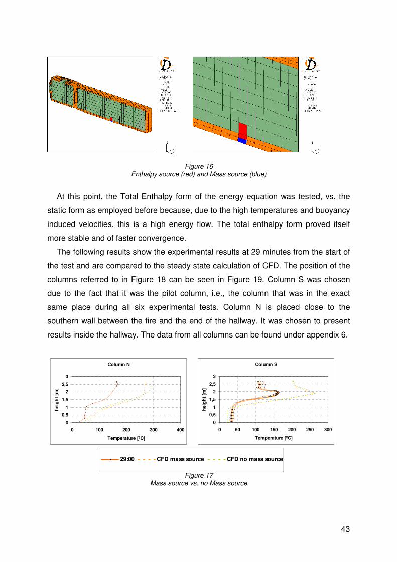
43
Figure 16
Enthalpy source (red) and Mass source (blue)
At this point, the Total Enthalpy form of the energy equation was tested, vs. the
static form as employed before because, due to the high temperatures and buoyancy
induced velocities, this is a high energy flow. The total enthalpy form proved itself
more stable and of faster convergence.
The following results show the experimental results at 29 minutes from the start of
the test and are compared to the steady state calculation of CFD. The position of the
columns referred to in Figure 18 can be seen in Figure 19. Column S was chosen
due to the fact that it was the pilot column, i.e., the column that was in the exact
same place during all six experimental tests. Column N is placed close to the
southern wall between the fire and the end of the hallway. It was chosen to present
results inside the hallway. The data from all columns can be found under appendix 6.
Column N
0
0,5
1
1,5
2
2,5
3
0 100 200 300 400
Temperature [ºC]
heig
ht
[m]
Column S
0
0,5
1
1,5
2
2,5
3
0 50 100 150 200 250 300
Temperature [ºC]
heig
ht
[m]
29:00 CFD mass source CFD no mass source
Figure 17
Mass source vs. no Mass source
44
The results show that the mass source causes the profile to approach the shape of
the experimental results.
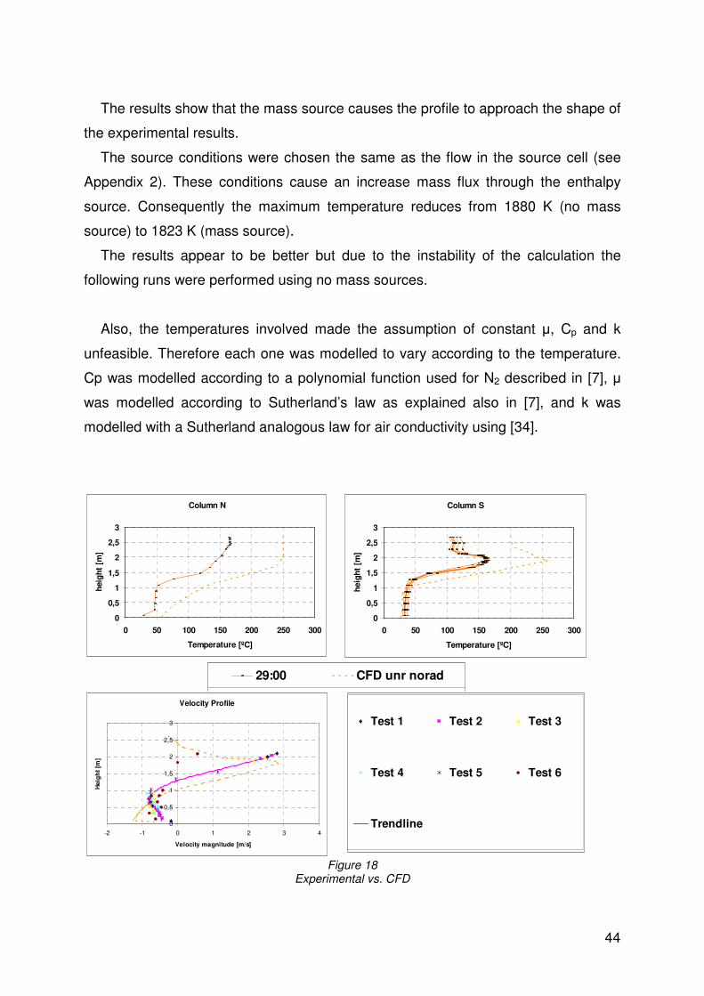
The source conditions were chosen the same as the flow in the source cell (see
Appendix 2). These conditions cause an increase mass flux through the enthalpy
source. Consequently the maximum temperature reduces from 1880 K (no mass
source) to 1823 K (mass source).
The results appear to be better but due to the instability of the calculation the
following runs were performed using no mass sources.
Also, the temperatures involved made the assumption of constant µ, Cp and k
unfeasible. Therefore each one was modelled to vary according to the temperature.
Cp was modelled according to a polynomial function used for N2 described in [7], µ
was modelled according to Sutherland’s law as explained also in [7], and k was
modelled with a Sutherland analogous law for air conductivity using [34].
Column N
0
0,5
1
1,5
2
2,5
3
0 50 100 150 200 250 300
Temperature [ºC]
heig
ht
[m]
Column S
0
0,5
1
1,5
2
2,5
3
0 50 100 150 200 250 300
Temperature [ºC]
heig
ht
[m]
C o lu mn Q
0
5
0 5 0 1 0 0 1 5 0 2 0 0 2 5 0 3 0 0 3 5 0
29:00 CFD unr norad
Velocity Profile
0
0,5
1
1,5
2
2,5
3
-2 -1 0 1 2 3 4
Velocity magnitude [m/s]
Heig
ht
[m]
0
5
-5 0 5
Test 1 Test 2 Test 3
Test 4 Test 5 Test 6
Trendline
Figure 18
Experimental vs. CFD

45
We can see from the charts that the basic physics appears to be respected and
the shape of the CFD solution resembles the experimental one. Temperature profiles
are nevertheless over-estimated and velocity results are somewhat good with a
height shift of around 25cm.
Figure 19
Column positions and Fire Source
3.5.2. Radiation
According to most references, radiation plays an important role in a fire driven
flow. The CFD solution showed that the results gain a shape closer to the
experimental solution through the dispersion of some of the energy throughout the
domain.
The radiation method used was the method of Discrete Ordinates. To model the
participating media, scalars were inserted in the stoichiometric proportion as they
would appear if the combustion was complete. The scalar sources and sinks
represent the consumption of O2 and the creation of CO2 and H2O. These scalars are
inserted in the domain through sources in the same cells as the enthalpy source.
Soot was included by creating another scalar and considered to be a percentage of
unburnt propane. In [5] we find the proposal that this value should be around 2.5 % of
the mass fuel injected. Also, in order for the combustion to form soot, part of the
propane does not burn, and so the power was reduced 2,5 % according to the soot
formation. Figure 20) shows the clear difference of having part of the energy passed
as radiation instead of convection.

46
Column N
0
0,5
1
1,5
2
2,5
3
0 50 100 150 200 250 300
Temperature [ºC]
heig
ht
[m]
Column S
0
0,5
1
1,5
2
2,5
3
0 50 100 150 200 250 300
Temperature [ºC]
heig
ht
[m]
C o lumn Q
T e m p e ra tu r29:00 CFD unr norad CFD unr rad
Figure 20
Experimental vs. CFD with and without radiation
A problem appeared when analyzing the mass fraction (scalar) values. They did
not add up to 1 in the entire domain. This was due to the fact that the denominator is
the density. Given that no mass is being injected in the domain this value is
underestimated and in the combustion products high influence zone this value will be
higher than 1. It could be proved that the highest error is of 3% directly in the scalar
source cells and decreases rapidly after. It is not possible to correct this without
increasing the complexity of the combustion and so this error is accepted.
We can see that the radiation results make the trends more realistic but all of the
CFD calculations overestimate temperature. (See appendix 7)
The velocity profile is almost equal to the non irradiative case.
Velocity Profile
0
0,5
1
1,5
2
2,5
3
-2 -1 0 1 2 3 4
Velocity magnitude [m/s]
Heig
ht
[m]
CFD unr rad
CFD unr norad
Figure 21
Velocity field difference between calculations with and without radiation modelling

47
3.5.3. Wall Treatment
3.5.3.1. Inner Structure Wall and Ceiling
The approach to wall modelling started through testing the sensitivity of the CFD
solution to transmissivity. In accordance, emissivity was reduced to 0,85 and
transmissivity increased from zero to 0,1.
Results showed almost no difference (Figure 22) which may lead us to think that
radiation plays an important role in the way that energy is distributed in the domain
but not so much as in the amount of energy that remains in the house in steady state.
The wall remained adiabatic.
Column N
0
0,5
1
1,5
2
2,5
3
0 50 100 150 200 250 300
Temperature [ºC]
heig
ht
[m]
Column S
0
0,5
1
1,5
2
2,5
3
0 50 100 150 200 250 300
Temperature [ºC]
heig
ht
[m]
C olu mn Q0
5
0 5 0
0
T e m p e ra tu r
29:00 CFD ref rad CFD ref rad trans
Figure 22
Solutions with and without Wall Transmissivity
The results of all columns and velocity profile can be found in Appendix 8.
To further increase reality a one dimensional equivalent conductivity was enforced
on the wall. This avoids the complexity of actually designing solid cells in the domain.
The thermal resistance R was set according to
[ ]WKmk
hR /2= ( 46 )
Where h is the local wall thickness and k is the conductivity for concrete according
to [5]. Outside temperature was also assumed to be constant at 288 Kelvin. As this
new wall treatment is independent of radiation, both calculations were performed:
with and without radiation.

48
On both cases we see that the difference between the experimental and CFD
calculations is reduced with the introduction of wall conduction. (Figure 23)
Column N
0
0,5
1
1,5
2
2,5
3
0 50 100 150 200 250 300
Temperature [ºC]
heig
ht
[m]
Column S
0
0,5
1
1,5
2
2,5
3
0 100 200 300 400
Temperature [ºC]
heig
ht
[m]
C o lumn Q
0
5
0 2 0 0 4 0 0
T e m p e ra tu r
29:00 CFD ref noradCFD ref rad CFD ref norad condCFD ref rad cond
Figure 23
Solutions with and without Wall Conduction
As before, the solution with radiation tends to reveal a temperature profile closer to
the experimental results. Full results can be found in appendix 9.
Another calculation was performed to check whether transmissivity has more
importance now that the walls are no longer adiabatic.
Column N
0
0,5
1
1,5
2
2,5
3
0 50 100 150 200 250 300
Temperature [ºC]
heig
ht
[m]
Column S
0
0,5
1
1,5
2
2,5
3
0 50 100 150 200 250 300
Temperature [ºC]
heig
ht
[m]
C olu mn N
5
29:00 CFD ref norad cond
CFD ref rad cond trans CFD ref rad cond
Figure 24 Solutions with Wall Conduction
This new solution is almost exactly like the one without transmissivity except in the
recirculation zone between the heat source and the closed end of the hallway. Even

49
then it is not clear if the solution found is better or worse than the one without
transmissivity and thus we decided to continue this study without it. The full results
can be found in appendix 10.
3.5.3.2. Floor
The thermal conductivity itself is not higher than a “normal” wall but the difference
in the calculation lies in the wall thickness for the Equivalent thermal resistance ( 46
). In addition, “outside temperature” which in this case is the ground temperature at a
certain depth also has a different value.
According to [5] the values set for Star were:
[ ][ ]CT
mh
mK
Wk
ext º20
0,3
.76,0
=
=
=
Two examples of these results are presented in Figure 25.
Column N
0
0,5
1
1,5
2
2,5
3
0 50 100 150 200 250
Temperature [ºC]
heig
ht
[m]
Column S
0
0,5
1
1,5
2
2,5
3
0 50 100 150 200 250
Temperature [ºC]
heig
ht
[m]
C olumn Q
0
5
0 5 0 1 0 0 1 5 0 2 0 0 2 5 0 3 0 0 3 5 0
29:00 CFD ref rad cond CFD ref rad cond3
Figure 25 Solution with (red) and without Floor Conduction (blue)
Although the only difference in both calculations is the floor conductivity, and even
that was set with a very high resistance, the solutions still differ. We can see that, for
column N, the shape of the temperature profile gained some more realism while for
column S the top part of the temperature profile has a undershoot providing a result
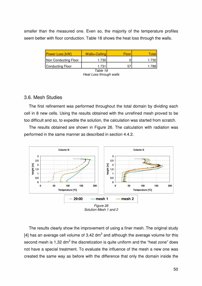
50
smaller than the measured one. Even so, the majority of the temperature profiles
seem better with floor conduction. Table 18 shows the heat loss through the walls.
Power Loss [kW] Walls+Ceiling Floor Total
Non Conducting Floor 1.730 0 1.730
Conducting Floor 1.731 57 1.788 Table 18
Heat Loss through walls
3.6. Mesh Studies
The first refinement was performed throughout the total domain by dividing each
cell in 8 new cells. Using the results obtained with the unrefined mesh proved to be
too difficult and so, to expedite the solution, the calculation was started from scratch.
The results obtained are shown in Figure 26. The calculation with radiation was
performed in the same manner as described in section 4.4.2.
Column N
0
0,5
1
1,5
2
2,5
3
0 50 100 150 200
Temperature [ºC]
heig
ht
[m]
Column S
0
0,5
1
1,5
2
2,5
3
0 50 100 150 200
Temperature [ºC]
heig
ht
[m]
0
5
0 5 0 0
T e mpe r a t ur e [ º C ]29:00 mesh 1 mesh 2
Figure 26 Solution Mesh 1 and 2
The results clearly show the improvement of using a finer mesh. The original study
[4] has an average cell volume of 3,42 dm3 and although the average volume for this
second mesh is 1,32 dm3 the discretization is quite uniform and the “heat zone” does
not have a special treatment. To evaluate the influence of the mesh a new one was
created the same way as before with the difference that only the domain inside the

51
house was refined, i.e. each cell inside the house originated 8 new cells. This way,
mesh 1 has a standard cell size of 30x30x30cm, mesh 2, 20x20x20cm and mesh 3,
10x10x10cm, with normal variations uptill a third of the standard cell size. Appendix
11 has the results of all three meshes.
Figure 27 shows the solution of all meshes. It can be seen that the most refined is
able to capture a more detailed solution but it grows further apart from the
experimental results when compared to the other meshes.
Column N
0
0,5
1
1,5
2
2,5
3
0 50 100 150 200 250
Temperature [ºC]
heig
ht
[m]
Column S
0
0,5
1
1,5
2
2,5
3
0 50 100 150 200 250
Temperature [ºC]
heig
ht
[m]
C o l u mn R
0
5
0 5 0 0
29:00 mesh 1 mesh 2 mesh 3
Figure 27
Solution Mesh 1, 2 and 3
3.7. Results
The following section shows the flow, temperature and visibility fields. The visibility
field was calculated using Jin’s method [26] according to the soot concentration.
The flow pattern moves around the house forming a large recirculation area
behind it. Moreover there are recirculation areas just before the structure’s openings
which affect the way the flow enters or leaves the house (Figure 28). In the window
this zone is sucked towards the inside of the house. The skylight, on the other hand
pushes it away from the house.

52
Figure 28
Flow field around the house top view (up) and side (down) – velocity vectors (arrows) and magnitude (colour)
Inside, Figure 29 shows that cold air is entering from the lower part of the window
and the skylight works like an exhaust letting the hot air escape the structure.
Figure 29
Flow and Temperature Fields in openings and door

53
The flow enters the hallway through the lower part of the door (Figure 29) and
rises and heats up as it reaches the heat source (Figure 30). While rising, it cools
down and spreads sideways in the ceiling creating a recirculation hot area in the east
part of the hallway and a hot layer travelling west. This hot layer above 80 ºC is
approximately 2,1m thick from the ceiling covering almost the entire hallway and
decreasing almost completely in the room (Figure 30 and Figure 31).
Figure 30
Rising Hot Flow
Figure 31
Hot and Cold Zones
The hot air buoyancy tends to maintain the soot in the hot zone and it does not
diffuse fast enough to spread to high quantities everywhere in the domain. Thus the
visibility is very small when standing in the hot layer and recirculation zones, but
improves when in the cold zone. Still, inside the hallway it does not go above 6m and
in the east side of hallway it is impossible to see through the fire zone (Figure 32).

54
Figure 32 Visibility
3.8. Conclusions
This model is capable to predict velocity and temperatures correctly with relatively
small differences towards the experimental data. The velocity profiles are a match
and temperatures have a typical overshoot around 10-20% difference towards the
experimental results.
As for the physical approach to this work one can state that to model an ISA
atmosphere one cannot use the Boussinesq approach for compressibility as it would
invert the density gradient.
Considering the fire source to be a “hot” inlet gives rise to problems on the
feasibility of the flow. In fact, for it to have an enthalpy source big enough to match
the expected from a fire it would be necessary to set the mass flux and/or the
temperature at unfeasible values. A source in the energy equation, on the other
hand, allows the simulation to reach the expected result with the penalty of having no
mass source. The latter can also be inserted in the Navier-Stokes equations but the
source conditions need to be tackled carefully for they can cause unrealistic
momentum sources.
Also, fire induced flows are often buoyancy dominated and thus naturally unstable.
Modelling of a large “outside” domain with wind is more likely to capture and
converge the flow calculation. Upwind discretization method for the momentum
equations is more sensitive to the domain size than MARS which produces more

55
consistent results for the same domains. Inlet BCs are preferable to pressure BCs
with the penalty of having to know more about the flow in that region. (section 3.4.3.)
Wall conductivity significantly reduces the amount of energy inside the structure.
This effect causes colder temperature profiles closer to the experimental data. On the
other hand, radiation does not change the total energy significantly but instead it
redistributes it to different temperatures profiles closer to the experimental shapes.
The model was also used to assess the importance of the external wind influence
on a fully developed indoor fire. In paper [36] it was concluded that wind has a non-
negligible effect and can cause significant differences in the smoke and temperature
distributions that varied, in the LNEC case, up to 40% in smoke concentration and
10% in average temperature.

56
4. AIRPORT CASE
4.1 Characterization
The zone of interest is located at the entrance of the international area just after
the current security checkpoint and ends after the travel shopping shop. Figure 33
illustrates the geometry. The fire will be simulated in the left escalator. (See Figure
34). This choice is due to historical precedents. In the past a fire occurred in that
zone due to the accumulation of combustible organic material underneath the
escalators that, probably ignited by either a spark or, at the time, a lit cigarette butt,
caused the production of smoke that led to the closing of the airport. The objective is
to assess what would be expected to happen in case of a new fire nowadays.
Figure 33
Geometry of interest zone - Four views (left) and level 4 isometric (right)
Figure 34
Zone of interest

57
4.2. Solid Modelling
The model was generated from the blueprints provided to us by ANA and height
was determined from pictures taken in loco. The software used was Star-Design.
Figure 33 depicts some pictures from the resulting model.
4.3. Mesh Generation
The mesh was generated using Pro-Am. The generation method was the same as
previously used in the LNEC case and stated in section 3.3.
Figure 35 Airport Mesh Views
The detail level comprised was the attempt to recreate as best as possible the
geometry of the zone in question. All the columns, AC systems, stores and shelves
were recreated. The domain has around 1.2 million cells and medium cell volume of
14 dm3. The fire zone and some zones with complex obstacles also reduce the
medium cell volume down to 1 dm3 per cell.

58
4.4. Boundary Conditions
This section presents the Boundary Conditions applied to the mesh as well as how
they were chosen and modelled. In the end the conditions imposed were inlets on the
AC systems, entrance at level 4 and door in level 5. The opening on level 5 was set
with a pressure BC (Figure 36 to Figure 44). The baffles in Figure 42 represent the
travel shopping alarms and, although they have little thickness they “stand in the
way” of the flow.
Figure 36
Boundary Conditions: Main Inlet
Figure 37
View from level 4 at Main Inlet

59
Figure 38
Boundary Conditions: AC level 4
Figure 39
Boundary Conditions: AC level 5
Figure 40
Level 5 and Swatch stand

60
Figure 41
Boundary Conditions: Door Outlet
Figure 42
Boundary Conditions: Baffles (Travel Shopping alarms)
Figure 43
View of Travel Shopping entrance and alarms

61
Figure 44
Boundary Conditions: Hallway Outlet
Initially the boundary conditions used were inlet at the end of level 4 and at the air
conditioning (AC) entrances. The two exits (the door and the hallway in level 5) were
set at constant pressure. The mass flow of the air conditioning entrances is know per
duct with 750 m3/h at level 4 and 1360 m3/h at level 5. The main entrance of level 4
was set with a total mass flux of 1/100 of the total mass flux entering the domain from
the AC entrances.
The results showed that near the main inlet zone unfeasible flows appear (Figure
45). Also it is known that both level 4 and 5 have complex AC systems continuously
pumping air into the domain. According to Eng. António Ramalhete there should be a
flow going from level 4 to 5. Therefore measurements were taken in the main inlet
zone of level 4 and it’s averaged values were applied in the inlet BC at level 4. These
measurements can be found on appendix 12.
Figure 45
Results near Main Inlet

62
The effect of the BC type on the service door in level 5 was also tested (Figure
41). This test consisted in having two calculations, one with a pressure BC (Case 01)
and another with an inlet BC (Case 02) with the same average mass flux as Case 01.
The results on both calculations were practically the same and Case 02 had higher
convergence rate, i.e., in order to obtain the same residual it took less time. The
difference in the variables is localized to the door and its influence to the surrounding
flow is negligible (Figure 46). From this study, Case 02 BCs were chosen to be
applied to the model.
Figure 46
Influence of Inlet vs. Pressure Boundary at Level 5 Door
4.5. Heat Source
The fire zone is located at the bottom of the escalator as shown in Figure 47 and
Figure 48.
Figure 47

63
Fire Zone
Figure 48
Escalator and stairs
The fire power was set as described in the section 2.3.1 with a power of
2/25 mkW spread over 22 m . This power was obtained from a mixture of polyester
and cotton fire powers according to [35]. As before, this routine is user programmed
and can be found in Appendix 1.
4.6. Numerical Aspects
This section describes the steps taken to converge the calculation.
This first step concerns the activation of the heat source. It was seen that it tends
to destabilize the calculation. This happens because each iteration is a pseudo time
step in the calculation and when the heat source is activated a “shock” is created
which may cause unrealistic values in density and temperatures leading to instability
or divergence. Thus, it was found through trial and error attempts that the best way to
do it is to begin with a smaller heat source for a few iterations (typically no more than
10 kW during 1 to 10 iterations). It may be necessary to increase the power slowly
when the heat source exceeds 100 kW as in the LNEC case. This offers the
calculation a sort of “jump start” needed to later stabilize the flow when using the heat
source at full power.
The second step refers to the quality of the solution. Due to the physical
phenomena and the mesh topology it happens that in some regions it is impossible to
lower the residuals as shown in Figure 49.

64
Figure 49
High Residual Cells
The source of these results is the relative sizes between cells, i.e., most of the
problematic cells belong to couples. A couple is a mechanism used so that the same
face of one cell (master) can be attached to the face of the different cells (slaves) as
depicted in Figure 50.
Also, these cells normally are the master of the couples. To correct this problem
the problematic cells were refined in order to have a relative size similar to the ones
attached to them.
Figure 50
Couple Example - Master (blue) and Slaves (White)
This step was very effective in reducing the mass residuals from 100 to 10-2.
Unfortunately, after applying this step a couple of times it becomes less effective and
if not done carefully it may even diverge the calculation. Also due to the instability of
the calculation it is always necessary to repeat the first step each time a refinement is
performed.
The third and last step concerns the relaxation factors (between 0 and 1) used in
the primary variables. These factors are used in both the solving matrix and the
predicted solution (or pseudo time step). The smaller they are the bigger the damping

65
of the oscillations. This is extremely effective to reduce numeric oscillations but
physics pays by damping the natural problem oscillations [7]. Therefore these factors
should not be used too freely.
The problem in this case is that, like most buoyant flows, the nature of the solution
is not steady. Therefore the goal is not to reach the steady state solution but to
achieve steadiness in the desired quantity or quantities. In this case the variable of
interest is the concentration of the soot (and thus the visibility).
After performing all three steps and reaching the relaxation factors down to 0,02
for pressure and 0,06 for the remaining variables it was seen that the desired level of
convergence would not be reached. Thus, “point” solutions were taken and
compared. Four of these solutions are shown in Figure 51 to Figure 54.
Figure 51 Visibility - Iteration 5.207
Figure 52 Visibility - Iteration 7.152

66
Figure 53 Visibility - Iteration 9.528
Figure 54 Visibility - Iteration 11.420
The results sequence shows that the solution does not seem to be stable but
oscillating. Nevertheless, these results also show that the solution, considering that
there is a stable solution, shall not be far apart from these results. In fact, any of the
previous solutions is feasible. Thus the calculation is terminated and the last iteration
will be analysed.

67
4.7. Results Analysis
This section describes the flow patterns obtained in case of an escalator fire past
the security checkpoint at Portela’s airport. Firstly the velocity flow patterns will be
shown followed by the temperature and concluding with visibility.
Figure 55 and show the flow patterns in Level 4. The air inserted in the domain by
the level 4 A/C curves towards level 5 and increases speed in the centre of the
hallway. There is a recirculation area evident in the upper left corner of the same
figure. This area does not seem to be affected by the A/C system. As the air flows to
Level 5, shown on Figure 56, we can see the fire induced flow in the left escalator.
The flow exits the area mostly through the passing before the travel shopping area
seen on Figure 57.
Figure 55
Velocity pattern (XY plane) at height 220 cm

68
Level 5 Left AC system
Left escalator (fire zone)
Right escalator
Level 5 Right AC system
Figure 56 Velocity patterns (ZY planes) of flow going from Level 4 to 5
Figure 57
Velocity pattern (XY plane) in Level 5
The temperature pattern is shown on Figure 58. It is visible that the temperature is
relatively low even close to the fire zone.

69
Figure 58
Temperature Pattern on Escalator section
From Figure 59 and Figure 60 we can see that visibility is reduced in the ceiling
and part of the travel shopping area. This means that the smoke would to travel to
the restaurant and boarding gates area.
Figure 59
Visibility pattern - escalator section

70
Figure 60
Visibility pattern - Level 5
4.8. Conclusions
The modelled fire situation seems to present little potential harm to people.
Temperatures do not rise away from the fire source and visibility does not decrease
to critical levels. Only in the dome the fog would be dense but at human height it
would be no more that a slight fog.
Nevertheless the natural flow pattern is predicted. Should the fire be more
powerful and/or toxic the situation can become dangerous for the people that stand in
the travel shopping store and would flea to the restaurant area. It is recommended
that exctraction ventilators be installed on this passing in order not to contaminate the
level 5 with whatever comes from level 4. This would produce flow isolation between
these two levels that separate security zones.

71
BIBLIOGRAPHY
1. Incropera, Frank P.; De Witt, David P., Fundamentals of Heat and Mass Transfer,
John Wiley & Sons, 5ª edição, 2002.
2. Zannetti, Paolo, Air Pollution Modelling – Theories, Computational Methods and
Available Software, Computational Mechanics Publications, UK, 1990
3. Drysdale, Dougal, An introduction to Fire Dynamics, Second Edition, John Wiley
and Sons, Inc., Great Britain, 2000
4. Viegas, J.C.G., Segurança contra incêndios em edifícios: modelação matemática
de incêndios e validação experimental, PhD Thesis, Instituto Superior Técnico,
Lisboa, 1999
5. Ozisik, M. Necati, Heat Transfer A Basic Approach, McGraw-Hill Book Company,
Singapore, 1985
6. Pereira, J. C. F., Silva F. P., Pereira, J. M. C., Coelho, P., Howard, R., Azevedo,
J., Farinha, F., IST Contribution to UPTUN, WP2, September to March 2005
7. STAR-CD Version 3.20 Methodology, CD adapco Group 2004.
8. Brederode, Vasco, Fundamentos de Aerodinâmica Incompressível, edição de
autor, 1997.
9. (Unknown), Lei nº 27/2006 – Aprova a Lei de Bases da Protecção Civil,
Assembleia da República, 2006.
10. Cox, G., Fire research in the 21st century, Fire Safety Journal, n. 25, pp. 337-353,
1999.
11. Emmons, H., Scientific progress on fire, Ann. Review Fluid Mechanics, n. 12, pp.
223-236, 1980.
12. Tieszen, S., On the Fluid Mechanics of Fires, Ann. Review Fluid Mechanics, n.
33, pp. 67-92, 1980.
13. Vogel, P., Simulation of Smoke Distribution and Extraction in Terminal 2 of
Munich Airport, 2006
14. Gobeau, N., Evaluation of CFD to predict smoke movement in complex enclosed
spaces, Health and Safety Executive, 2004
15. Liu, Y., Comparison of a CFD Fire Model against a Ventilated Fire Experiment in
an Enclosure, The international journal of Ventilation, Volume 3 Number 2, 2004

72
16. Yeoh, G.H., Fire and smoke distribution in a two-room compartment structure,
International Journal of Numerical Methods for Heat & Fluid Flow, volume 12
Number 2 pp.178-194, 2002
17. Waterson, N.P., Modelling Fire and Smoke Spread in Enclosed Spaces, 1st
QNET-CFD Workshop on Quality and Trust in CFD, 2001
18. Grandison, A.J., Fire Modelling Standards/Benchmark, Fire Safety Engineering
Group, 2001
19. Schabacker, J., CFD study of Temperature and Smoke Distribution in a Railway
Tunnel with Natural Ventilation System.
20. Hwang, C.C., CFD Modelling of Smoke Reversal, Pittsburgh Research Laboratory
21. Luo, M. Application of Field Model and Two-zone Model to Flashover fires in a
Full-scale Multi-room Single Level Building, Fire Safety Journal, 1997
22. Prandtl, L., On the Role of Turbulence in Technical Hydrodynamics, Proceedings
of the World Engineering Congress, Tóquio, vol. 6, pp. 495–507, 1931
23. Modest, M.F., Radiative Heat Transfer, McGraw-Hill, New York. 1993
24. Siegel, R., and Howell, J., Thermal Radiation Heat Transfer, Hemisphere
Publishing, Washington, 1992
25. Jin, T., Visibility Through Fire Smoke, in Main Reports on Production, Movements
and Control in Buildings, Japanese Association of Fire Science and Engineering,
pp. 100 –153, 1974.
26. Jin, T., Visibility Through Fire Smoke, Report of the Fire Research Institute of
Japan, 5 (2), pp. 12–18, 1975.
27. Jin, T., Visibility Through Fire Smoke, Journal of Fire and Flammability, Volume 9,
No.2, pp. 135–155, April 1978.
28. Jin, T., Irritating Effects of Fire Smoke on Visibility, Fire Science and Technology,
Volume 5, No. 1, pp. 79–90, 1985.
29. Klote, J.H., and J.A. Milke, Principles of Smoke Management, American Society
of Heating, Refrigerating, and Air Conditioning Engineers, Inc. (ASHRAE), and
Society of Fire Protection Engineers (SFPE), ASHRAE Special Publication, 2002.
30. Seader, J. and I. Einhorn, Some Physical, Chemical, Toxicological, and
Physiological Aspects of Fire Smokes, National Science Foundation (NSF)
Report, Utah University, 1976.

73
31. Steiner, A.J., Method of Fire Hazard Classification of Building Materials, ASTM
Bulletin, American Society of Testing and Materials (ASTM), Philadelphia,
Pennsylvania, pp. 12–18, March 1943.
32. Barlow, R., Radiation Models, International Workshop on Measurement and
Computation of Turbulent Nonpremixed Flames, 2003.
33. Houghton, E.L. and Carruthers N. B., Wind Forces on Buildings and Structures an
introduction, 1976, Edward Arnold Ltd, London
34. Sandia National Laboratories, Radiation Models, 2003
35. Ofodike A. Ezekoye and Kenneth R. Diller, A Model for Assessing Ignition, Flame
Spread, and Burn Hazard Potential of a Multilayered Jacket, Journal of Burn Care
& Research, pp 487-495, August 2006
36. Magalhães, N.P., Marques, N.P.C. and Pereira, J.C.P, External wind influence on
a fully developed indoor fire, LASEF, Advanced Research Workshop on “Fire
Computer Modeling”, Santander, 2007

74
Appendixes

75
Appendix 1. Heat Source subroutine “sorent.f” for both LNEC and Airport Cases
C**********************************
SUBROUTINE SORENT(S1P,S2P)
C Source-term for enthalpy
C**********************************
C------------------
C STAR VERSION 3.24.000
C-------------------
INCLUDE 'comdb.inc'
COMMON/USR001/INTFLG(100)
INCLUDE 'usrdat.inc'
DIMENSION SCALAR(50)
EQUIVALENCE( UDAT12(001),
ICTID )
EQUIVALENCE( UDAT03(001), CON
)
EQUIVALENCE( UDAT03(019),
VOLP )
EQUIVALENCE( UDAT04(001), CP )
EQUIVALENCE( UDAT04(002), DEN
)
EQUIVALENCE( UDAT04(003), ED )
EQUIVALENCE( UDAT04(004), HP )
EQUIVALENCE( UDAT04(006), P )
EQUIVALENCE( UDAT04(008), TE )
EQUIVALENCE( UDAT04(009),
SCALAR(01) )
EQUIVALENCE( UDAT04(059), U )
EQUIVALENCE( UDAT04(060), V )
EQUIVALENCE( UDAT04(061), W )
EQUIVALENCE( UDAT04(062),
VISM )
EQUIVALENCE( UDAT04(063), VIST
)
EQUIVALENCE( UDAT04(007), T )
EQUIVALENCE( UDAT04(067), X )
EQUIVALENCE( UDAT04(068), Y )
EQUIVALENCE( UDAT04(069), Z )
C------------------
C
C This subroutine enables the user to
specify a source term (per unit volume) for
enthalpy in linearized form:
C
C Source = S1P-S2P*T, (W/m3)
C
C in an arbitrary manner.
C
C If temperature is to be fixed to a given
value T, then the following may be used:
C
C S1P=GREAT*T
C S2P=GREAT,
C
C where T can be a constant or an
arbitrary function of the parameters in the
parameter list.
C
C ** Parameters to be returned to STAR:
S1P,S2P
C
C-------------------C
if ((ictid.eq.4)) then
c in KW
FirePower=173.3
c volume of ictid 4
totalvolume=37045.5/1000000
s1p=FirePower*1000/totalvolume
c s1p=4678031.07
endif
RETURN
END
C

76
Appendix 2. Mass Source subroutine “fluinj.f”
C*******
SUBROUTINE
FLUINJ(FLUXI,UI,VI,WI,TEI,EDI,TI,SCI
NJ,IPMASS)
C Fluid injection
C***
C-----------
C STAR VERSION 3.24.000
*
C----------------
INCLUDE 'comdb.inc'
DIMENSION SCINJ(50)
COMMON/USR001/INTFLG(100)
INCLUDE 'usrdat.inc'
DIMENSION SCALAR(50)
EQUIVALENCE( UDAT12(001),
ICTID )
EQUIVALENCE( UDAT03(001), CON
)
EQUIVALENCE( UDAT03(019),
VOLP )
EQUIVALENCE( UDAT04(001), CP )
EQUIVALENCE( UDAT04(002), DEN
)
EQUIVALENCE( UDAT04(003), ED )
EQUIVALENCE( UDAT04(005), PR )
EQUIVALENCE( UDAT04(008), TE )
EQUIVALENCE( UDAT04(009),
SCALAR(01) )
EQUIVALENCE( UDAT04(059), U )
EQUIVALENCE( UDAT04(060), V )
EQUIVALENCE( UDAT04(061), W )
EQUIVALENCE( UDAT04(062),
VISM )
EQUIVALENCE( UDAT04(063), VIST
)
EQUIVALENCE( UDAT04(007), T )
EQUIVALENCE( UDAT04(067), X )
EQUIVALENCE( UDAT04(068), Y )
EQUIVALENCE( UDAT04(069), Z )
C-----------------
C This subroutine enables the user to
specify fluid injection (addition or removal)
into live cells. In the case of mass removal
(sink), only the mass flux (FLUXI) can be
specified. In the case of mass addition
(source), the fluid will bring all its user-
specified properties (momentum, turbulence,
temperature and concentrations). Zero will
be assumed for omitted properties.
C
C ** Parameters to be returned to STAR:
C (Sink) FLUXI (<0)
C (Source) FLUXI
(>0),UI,VI,WI,TEI,EDI,TI,
C SCINJ,IPMASS
C
C IPMASS is an interphase mass transfer
indicator used in Eulerian two-phase (E2P)
simulations only. The default value, passed
from STAR to FLUINJ, is always zero.
C IPMASS=0: no interphase heat transfer
- the mass sources specified
C in FLUINJ are independent for each
phase.
C IPMASS=1: the phases are exchanging
mass - the mass source specified is directed
from one phase into the other phase. For
more information, please refer to the E2P
sections of the manuals.
IF(ICTID.EQ.3) THEN
C Injection
C The mass flux should be 3,7387 g/s of
propane. The cell volume is 12180,1 cm^3.
c The correction of mass to mols is given by
the molecular weight ratios
M(C3H8)=44,1g/mol M(air)=28,9 g/mol
c The air equivvalent mass flux is then 2,45
g/s
c Fluxi is then 2,45/(12180,1/1000)
C Disregard last comment for the weight of
C and H is necessary to be in accordance
with the scalar sources
c FLUXI=0.2012
c Volume of ICTID 3 is 12180,1 cm3

77
TotalVolume = 12180.1/1000000
c in KW
FirePower=173.3
c mass flux of C3H8
fluxC3H8=FirePower/46353.
FLUXI=fluxC3H8/TotalVolume
C Same propertiies as the existing flow
UI=U
VI=V
WI=W
TEI=TE
EDI=ED
TI=T
SCINJ(1)=1.0
scalar(1)=0.23310
scalar(2)=0.76690
ENDIF
RETURN
END
C

78
Appendix 3. Scalar Sources subroutine “sorsca.f”
SUBROUTINE SORSCA(S1P,S2P)
C Source-term for scalar species
C*****
C------------
C STAR VERSION 3.24.000
*
C-------------------
INCLUDE 'comdb.inc'
COMMON/USR001/INTFLG(100)
INCLUDE 'usrdat.inc'
DIMENSION SCALAR(50)
EQUIVALENCE( UDAT12(001),
ICTID )
EQUIVALENCE( UDAT03(001), CON
)
EQUIVALENCE( UDAT03(002), TAU
)
EQUIVALENCE( UDAT03(009),
DUDX )
EQUIVALENCE( UDAT03(010),
DVDX )
EQUIVALENCE( UDAT03(011),
DWDX )
EQUIVALENCE( UDAT03(012),
DUDY )
EQUIVALENCE( UDAT03(013),
DVDY )
EQUIVALENCE( UDAT03(014),
DWDY )
EQUIVALENCE( UDAT03(015),
DUDZ )
EQUIVALENCE( UDAT03(016),
DVDZ )
EQUIVALENCE( UDAT03(017),
DWDZ )
EQUIVALENCE( UDAT03(019),
VOLP )
EQUIVALENCE( UDAT04(001), CP )
EQUIVALENCE( UDAT04(002), DEN
)
EQUIVALENCE( UDAT04(003), ED )
EQUIVALENCE( UDAT04(004), HP )
EQUIVALENCE( UDAT04(006), P )
EQUIVALENCE( UDAT04(008), TE )
EQUIVALENCE( UDAT04(009),
SCALAR(01) )
EQUIVALENCE( UDAT04(059), U )
EQUIVALENCE( UDAT04(060), V )
EQUIVALENCE( UDAT04(061), W )
EQUIVALENCE( UDAT04(062),
VISM )
EQUIVALENCE( UDAT04(063), VIST
)
EQUIVALENCE( UDAT04(007), T )
EQUIVALENCE( UDAT04(067), X )
EQUIVALENCE( UDAT04(068), Y )
EQUIVALENCE( UDAT04(069), Z )
EQUIVALENCE( UDAT09(001), IS )
C--------------------
C This subroutine enables the user to
specify source terms (per unit
C volume) for species in linearized form:
C
C Source = S1P-S2P*SCALAR(IS),
(kg/sm3)
C
C in an arbitrary manner.
C
C If the species is to be fixed to a given
value SCI, then the following may be used:
C
C S1P=GREAT*SCI
C S2P=GREAT,
C
C where SCI can be a constant or an
arbitrary function of the parameters in
parameter list.
C
C ** Parameters to be returned to STAR:
S1P,S2P
C
C-------------------
if ((ictid.eq.4)) then
c in KW
FirePower=173.3
c mass flux of C3H8
fluxC3H8=FirePower/46353.

79
weightProp=44.00
TotalfluxMol =
fluxC3H8/weightProp
c volume of ictid 4
totalvolume=37045.5/1000000
c volume fraction of total volume -
unnecessary for s1p will be multiplied by
volp
C fractionv = volp/totalvolume
c------------------ Mass fraction of fuel
unburnt and transported as soot
sootfraction = 0.025
fluxMol = (1-
sootfraction)*TotalfluxMol
c print*,'TotalfluxMol, fluxMol, is
',TotalfluxMol, fluxMol, is
c------------------ Soot production
if (is.eq.5) then
auxiliar = fluxC3H8*sootfraction
s1p = auxiliar/totalvolume
endif
c oxygen consumtion
if (is.eq.1) then
weight = 32.
auxiliar = -fluxMol*weight*5.
s1p = auxiliar/totalvolume
endif
c CO2 production
if (is.eq.3) then
weight = 44.
auxiliar = fluxMol*weight*3.
s1p = auxiliar/totalvolume
c print*,'CO2 flux ',auxiliar
endif
c Water production
if (is.eq.4) then
weight = 18.
auxiliar = fluxMol*weight*4.
s1p = auxiliar/totalvolume
c print*,'H2O flux ',auxiliar
endif
endif
c out of ictid 4
RETURN
END

80
Appendix 4. Radiation Properties subroutine “radpro.f”
C*****
SUBROUTINE
RADPRO(COABS,COSCAT)
C Gaseous radiation properties
C******
C STAR VERSION 3.24.000
C--------------------
INCLUDE 'comdb.inc'
COMMON/USR001/INTFLG(100)
INCLUDE 'usrdat.inc'
DIMENSION SCALAR(50)
EQUIVALENCE( UDAT04(001), CP )
EQUIVALENCE( UDAT04(002), DEN
)
EQUIVALENCE( UDAT04(003), ED )
EQUIVALENCE( UDAT04(004), H )
EQUIVALENCE( UDAT04(005), PR )
EQUIVALENCE( UDAT04(006), P )
EQUIVALENCE( UDAT04(008), TE )
EQUIVALENCE( UDAT04(009),
SCALAR(01) )
EQUIVALENCE( UDAT04(059), U )
EQUIVALENCE( UDAT04(060), V )
EQUIVALENCE( UDAT04(061), W )
EQUIVALENCE( UDAT04(062),
VISM )
EQUIVALENCE( UDAT04(063), VIST
)
EQUIVALENCE( UDAT04(007), T )
EQUIVALENCE( UDAT04(067), X )
EQUIVALENCE( UDAT04(068), Y )
EQUIVALENCE( UDAT04(069), Z )
EQUIVALENCE( UDAT12(001),
ICTID )
DIMENSION CH2O(0:5)
DIMENSION CCO2(0:5)
DIMENSION MOL_MASS(1:4)
DATA CH2O/-0.23093,-
1.12390,9.41530,-2.99880,0.51382,-
1.86840E-05/
DATA CCO2/18.741,-
121.310,273.500,-194.050,56.310,-5.8169/
DATA MOL_MASS/32,28,44,18/
C---------
C This subroutine enables the user to
specify gaseous radiation properties.
C ** Parameters to be returned to STAR:
COABS,COSCAT
c total moles
RMIX=0.0
DO J=1,4
RMIX=RMIX+SCALAR(J)/MOL_
MASS(J)
ENDDO
c mol fractions
XH2O=SCALAR(4)/MOL_MASS(4)*(1.0/
RMIX)
XCO2=SCALAR(3)/MOL_MASS(3)*(1.0/
RMIX)
AKH2O=CH2O(0)
AKCO2=CCO2(0)
DO J=1,5
AKH20=AKH20+CH2O(J)*(1000.0/
T)**J
AKCO2=AKCO2+CCO2(J)*(1000.0
/T)**J
ENDDO
C--------SooT-------------
CM=SCALAR(5)*DEN
AKSOOT=1232.4*CM*(1+0.00048*(T-
2000))
c Considering constant pressure for 1
atm
COABS=AKH2O*XH2O+AKCO2*XCO2
+AKSOOT
COSCAT=0.0
RETURN
END
C

Appendix 5. Jin’s method ProStar source code
oper getc conc 4 5
oper sdiv 0.000396 4 4
csca,14,user,0.360695,15,,standard
pldisplay,on,all

Appendix 6. Experimental Results vs. Enthalpy Source and Enthalpy + Mass Source
Column A
0
0,5
1
1,5
2
2,5
3
0 100 200 300 400
Temperature [ºC]
he
igh
t [m
]
Column B
0
0,5
1
1,5
2
2,5
3
0 100 200 300 400
Temperature [ºC]
he
igh
t [m
]
Column C
0
0,5
1
1,5
2
2,5
3
0 100 200 300
Temperature [ºC]
he
igh
t [m
]
Column G
0
0,5
1
1,5
2
2,5
3
0 100 200 300 400
Temperature [ºC]
he
igh
t [m
]
Column H
0
0,5
1
1,5
2
2,5
3
0 100 200 300 400
Temperature [ºC]
he
igh
t [m
]
Column I
0
0,5
1
1,5
2
2,5
3
0 100 200 300
Temperature [ºC]
he
igh
t [m
]
Column M
0
0,5
1
1,5
2
2,5
3
0 100 200 300 400
Temperature [ºC]
he
igh
t [m
]
Column N
0
0,5
1
1,5
2
2,5
3
0 100 200 300 400
Temperature [ºC]
he
igh
t [m
]
Column O
0
0,5
1
1,5
2
2,5
3
0 100 200 300
Temperature [ºC]
he
igh
t [m
]

83
Column D
0
0,5
1
1,5
2
2,5
3
0 100 200 300 400
Temperature [ºC]
he
igh
t [m
]Column E
0
0,5
1
1,5
2
2,5
3
0 100 200 300 400
Temperature [ºC]
he
igh
t [m
]
Column F
0
0,5
1
1,5
2
2,5
3
0 100 200 300 400
Temperature [ºC]
he
igh
t [m
]
Column J
0
0,5
1
1,5
2
2,5
3
0 100 200 300 400
Temperature [ºC]
he
igh
t [m
]
Column K
0
0,5
1
1,5
2
2,5
3
0 100 200 300 400
Temperature [ºC]
he
igh
t [m
]
Column L
0
0,5
1
1,5
2
2,5
3
0 100 200 300 400
Temperature [ºC]
he
igh
t [m
]
Column P
0
0,5
1
1,5
2
2,5
3
0 100 200 300 400
Temperature [ºC]
he
igh
t [m
]
Column Q
0
0,5
1
1,5
2
2,5
3
0 100 200 300 400
Temperature [ºC]
he
igh
t [m
]
Column R
0
0,5
1
1,5
2
2,5
3
0 100 200 300 400
Temperature [ºC]
he
igh
t [m
]

84
Column S
0
0,5
1
1,5
2
2,5
3
0 100 200 300
Temperature [ºC]
heig
ht
[m]
0
5
0 100 200 300 400
Temperature [ºC]
heig
ht
[m]
29:00 CFD mass source CFD no mass source
Velocity Profile
0
0,5
1
1,5
2
2,5
3
-2 -1 0 1 2 3 4
Velocity magnitude [m/s]
Heig
ht
[m]
CFD no mass source
CFD mass source
Test 1
Test 2
Test 3
Test 4
Test 5
Test 6
Experimental Trendline
Experimental Trendline

85
Appendix 7. Experimental Results vs. Radiative and non-radiative media
Colunmn A
0
0,5
1
1,5
2
2,5
3
0 100 200 300
Temperature [ºC]
he
igh
t [m
]
Column B
0
0,5
1
1,5
2
2,5
3
0 100 200 300
Temperature [ºC]
he
igh
t [m
]
Coluna C
0
0,5
1
1,5
2
2,5
3
0 100 200 300
Temperatura [ºC]
co
tas [
m]
Column G
0
0,5
1
1,5
2
2,5
3
0 100 200 300
Temperature [ºC]
he
igh
t [m
]
Column H
0
0,5
1
1,5
2
2,5
3
0 100 200 300
Temperature [ºC]
he
igh
t [m
]
Column I
0
0,5
1
1,5
2
2,5
3
0 100 200 300
Temperature [ºC]
he
igh
t [m
]
Column M
0
0,5
1
1,5
2
2,5
3
0 100 200 300
Temperature [ºC]
he
igh
t [m
]
Column N
0
0,5
1
1,5
2
2,5
3
0 100 200 300
Temperature [ºC]
he
igh
t [m
]
Column O
0
0,5
1
1,5
2
2,5
3
0 100 200 300
Temperature [ºC]h
eig
ht
[m]

86
Column D
0
0,5
1
1,5
2
2,5
3
0 100 200 300 400
Temperature [ºC]
he
igh
t [m
]Column E
0
0,5
1
1,5
2
2,5
3
0 100 200 300 400
Temperature [ºC]
he
igh
t [m
]
Column F
0
0,5
1
1,5
2
2,5
3
0 100 200 300 400
Temperature [ºC]
he
igh
t [m
]
Column J
0
0,5
1
1,5
2
2,5
3
0 100 200 300 400
Temperature [ºC]
he
igh
t [m
]
Column K
0
0,5
1
1,5
2
2,5
3
0 100 200 300 400
Temperature [ºC]
he
igh
t [m
]
Column L
0
0,5
1
1,5
2
2,5
3
0 100 200 300 400
Temperature [ºC]
he
igh
t [m
]
Column P
0
0,5
1
1,5
2
2,5
3
0 100 200 300 400
Temperature [ºC]
he
igh
t [m
]
Column Q
0
0,5
1
1,5
2
2,5
3
0 100 200 300 400
Temperature [ºC]
he
igh
t [m
]
Column R
0
0,5
1
1,5
2
2,5
3
0 100 200 300 400
Temperature [ºC]
he
igh
t [m
]

87
Column S
0
0,5
1
1,5
2
2,5
3
0 100 200 300
Temperature [ºC]
heig
ht
[m]
Column Q
0
0,5
1
1,5
2
2,5
3
0 200 400
Temperature [ºC]
heig
ht
[m]
29:00 CFD unr norad CFD unr rad
Velocity Profile
0
0,5
1
1,5
2
2,5
3
-2 -1 0 1 2 3 4
Velocity magnitude [m/s]
Heig
ht
[m]
CFD unr rad
CFD unr norad
Test 1
Test 2
Test 3
Test 4
Test 5
Test 6
Experimental Trendline
Experimental Trendline

88
Appendix 8. Experimental Results vs. Transmissible and non-Transmissible Walls
Colunmn A
0
0,5
1
1,5
2
2,5
3
0 100 200 300
Temperature [ºC]
he
igh
t [m
]
Column B
0
0,5
1
1,5
2
2,5
3
0 100 200 300
Temperature [ºC]
he
igh
t [m
]
Coluna C
0
0,5
1
1,5
2
2,5
3
0 100 200 300 400
Temperatura [ºC]
co
tas [
m]
Column G
0
0,5
1
1,5
2
2,5
3
0 100 200 300
Temperature [ºC]
he
igh
t [m
]
Column H
0
0,5
1
1,5
2
2,5
3
0 100 200 300
Temperature [ºC]
he
igh
t [m
]
Column I
0
0,5
1
1,5
2
2,5
3
0 100 200 300 400
Temperature [ºC]
he
igh
t [m
]
Column M
0
0,5
1
1,5
2
2,5
3
0 100 200 300
Temperature [ºC]
he
igh
t [m
]
Column N
0
0,5
1
1,5
2
2,5
3
0 100 200 300
Temperature [ºC]
he
igh
t [m
]
Column O
0
0,5
1
1,5
2
2,5
3
0 100 200 300 400
Temperature [ºC]h
eig
ht
[m]

89
Column D
0
0,5
1
1,5
2
2,5
3
0 100 200 300 400
Temperature [ºC]
he
igh
t [m
]Column E
0
0,5
1
1,5
2
2,5
3
0 100 200 300 400
Temperature [ºC]
he
igh
t [m
]
Column F
0
0,5
1
1,5
2
2,5
3
0 100 200 300 400
Temperature [ºC]
he
igh
t [m
]
Column J
0
0,5
1
1,5
2
2,5
3
0 100 200 300 400
Temperature [ºC]
he
igh
t [m
]
Column K
0
0,5
1
1,5
2
2,5
3
0 100 200 300 400
Temperature [ºC]
he
igh
t [m
]
Column L
0
0,5
1
1,5
2
2,5
3
0 100 200 300
Temperature [ºC]
he
igh
t [m
]
Column P
0
0,5
1
1,5
2
2,5
3
0 100 200 300 400
Temperature [ºC]
he
igh
t [m
]
Column Q
0
0,5
1
1,5
2
2,5
3
0 100 200 300 400
Temperature [ºC]
he
igh
t [m
]
Column R
0
0,5
1
1,5
2
2,5
3
0 100 200 300 400
Temperature [ºC]
he
igh
t [m
]

90
Column S
0
0,5
1
1,5
2
2,5
3
0 100 200 300
Temperature [ºC]
heig
ht
[m]
Column Q
0
0,5
1
1,5
2
2,5
3
0 200 400
Temperature [ºC]
heig
ht
[m]
29:00 CFD ref rad CFD ref rad trans
Velocity Profile
0
0,5
1
1,5
2
2,5
3
-2 -1 0 1 2 3 4
Velocity magnitude [m/s]
He
igh
t [m
]
CFD ref rad trans
CFD ref rad
Test 1
Test 2
Test 3
Test 4
Test 5
Test 6
Experimental Trendline
Experimental Trendline
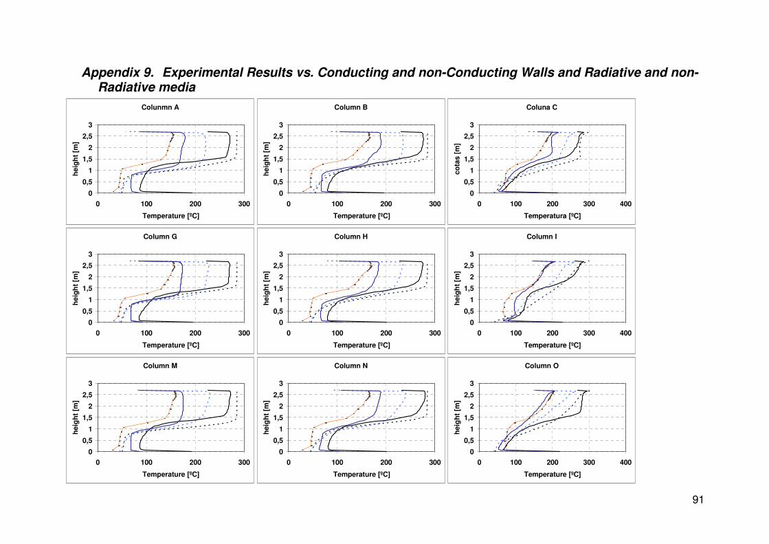
91
Appendix 9. Experimental Results vs. Conducting and non-Conducting Walls and Radiative and non-Radiative media
Colunmn A
0
0,5
1
1,5
2
2,5
3
0 100 200 300
Temperature [ºC]
he
igh
t [m
]
Column B
0
0,5
1
1,5
2
2,5
3
0 100 200 300
Temperature [ºC]
he
igh
t [m
]
Coluna C
0
0,5
1
1,5
2
2,5
3
0 100 200 300 400
Temperatura [ºC]
co
tas [
m]
Column G
0
0,5
1
1,5
2
2,5
3
0 100 200 300
Temperature [ºC]
he
igh
t [m
]
Column H
0
0,5
1
1,5
2
2,5
3
0 100 200 300
Temperature [ºC]
he
igh
t [m
]
Column I
0
0,5
1
1,5
2
2,5
3
0 100 200 300 400
Temperature [ºC]
he
igh
t [m
]
Column M
0
0,5
1
1,5
2
2,5
3
0 100 200 300
Temperature [ºC]
he
igh
t [m
]
Column N
0
0,5
1
1,5
2
2,5
3
0 100 200 300
Temperature [ºC]
he
igh
t [m
]
Column O
0
0,5
1
1,5
2
2,5
3
0 100 200 300 400
Temperature [ºC]
he
igh
t [m
]

92
Column D
0
0,5
1
1,5
2
2,5
3
0 100 200 300 400
Temperature [ºC]
he
igh
t [m
]Column E
0
0,5
1
1,5
2
2,5
3
0 100 200 300 400
Temperature [ºC]
he
igh
t [m
]
Column F
0
0,5
1
1,5
2
2,5
3
0 100 200 300 400
Temperature [ºC]
he
igh
t [m
]
Column J
0
0,5
1
1,5
2
2,5
3
0 100 200 300 400
Temperature [ºC]
he
igh
t [m
]
Column K
0
0,5
1
1,5
2
2,5
3
0 100 200 300 400
Temperature [ºC]
he
igh
t [m
]
Column L
0
0,5
1
1,5
2
2,5
3
0 100 200 300 400
Temperature [ºC]
he
igh
t [m
]
Column P
0
0,5
1
1,5
2
2,5
3
0 100 200 300 400
Temperature [ºC]
he
igh
t [m
]
Column Q
0
0,5
1
1,5
2
2,5
3
0 100 200 300 400
Temperature [ºC]
he
igh
t [m
]
Column R
0
0,5
1
1,5
2
2,5
3
0 100 200 300 400
Temperature [ºC]
he
igh
t [m
]

93
Column S
0
0,5
1
1,5
2
2,5
3
0 100 200 300 400
Temperature [ºC]
heig
ht
[m]
Column Q
0
0,5
1
1,5
2
2,5
3
0 200 400
Temperature [ºC]
heig
ht
[m]
29:00 CFD ref norad
CFD ref rad CFD ref norad cond
CFD ref rad cond
Velocity Profile
0
0,5
1
1,5
2
2,5
3
-2 -1 0 1 2 3 4
Velocity magnitude [m/s]
Heig
ht
[m]
CFD ref rad cond trans
CFD ref norad conduc
CFD ref rad
CFD ref norad
Test 1
Test 2
Test 3
Test 4
Test 5
Test 6
Experimental Trendline
Experimental Trendline

94
Appendix 10. Experimental Results vs. Transmissible and non Transmissible conducting walls
Colunmn A
0
0,5
1
1,5
2
2,5
3
0 50 100 150 200 250
Temperature [ºC]
he
igh
t [m
]
Column B
0
0,5
1
1,5
2
2,5
3
0 50 100 150 200 250
Temperature [ºC]
he
igh
t [m
]
Coluna C
0
0,5
1
1,5
2
2,5
3
0 100 200 300
Temperatura [ºC]
co
tas [
m]
Column G
0
0,5
1
1,5
2
2,5
3
0 50 100 150 200 250
Temperature [ºC]
he
igh
t [m
]
Column H
0
0,5
1
1,5
2
2,5
3
0 50 100 150 200 250
Temperature [ºC]
he
igh
t [m
]
Column I
0
0,5
1
1,5
2
2,5
3
0 100 200 300
Temperature [ºC]
he
igh
t [m
]
Column M
0
0,5
1
1,5
2
2,5
3
0 50 100 150 200 250
Temperature [ºC]
he
igh
t [m
]
Column N
0
0,5
1
1,5
2
2,5
3
0 100 200 300
Temperature [ºC]
he
igh
t [m
]
Column O
0
0,5
1
1,5
2
2,5
3
0 100 200 300
Temperature [ºC]h
eig
ht
[m]

95
Column D
0
0,5
1
1,5
2
2,5
3
0 100 200 300
Temperature [ºC]
he
igh
t [m
]Column E
0
0,5
1
1,5
2
2,5
3
0 100 200 300
Temperature [ºC]
he
igh
t [m
]
Column F
0
0,5
1
1,5
2
2,5
3
0 100 200 300
Temperature [ºC]
he
igh
t [m
]
Column J
0
0,5
1
1,5
2
2,5
3
0 100 200 300
Temperature [ºC]
he
igh
t [m
]
Column K
0
0,5
1
1,5
2
2,5
3
0 100 200 300
Temperature [ºC]
he
igh
t [m
]
Column L
0
0,5
1
1,5
2
2,5
3
0 100 200 300
Temperature [ºC]
he
igh
t [m
]
Column P
0
0,5
1
1,5
2
2,5
3
0 100 200 300
Temperature [ºC]
he
igh
t [m
]
Column Q
0
0,5
1
1,5
2
2,5
3
0 100 200 300
Temperature [ºC]
he
igh
t [m
]
Column R
0
0,5
1
1,5
2
2,5
3
0 100 200 300
Temperature [ºC]
he
igh
t [m
]

96
Column S
0
0,5
1
1,5
2
2,5
3
0 100 200 300
Temperature [ºC]
heig
ht
[m]
Column Q
0
0,5
1
1,5
2
2,5
3
0 200 400
Temperature [ºC]
heig
ht
[m]
29:00 CFD ref norad cond
CFD ref rad cond trans CFD ref rad cond
Velocity Profile
0
0,5
1
1,5
2
2,5
3
-2 -1 0 1 2 3 4
Velocity magnitude [m/s]
Heig
ht
[m]
CFD ref rad cond trans
CFD ref norad conduc
CFD ref norad
Test 1
Test 2
Test 3
Test 4
Test 5
Test 6
Experimental Trendline
Experimental Trendline

97
Appendix 11. Experimental Results vs. Mesh 1, 2 and 3
Column A
0
0,5
1
1,5
2
2,5
3
0 50 100 150 200
Temperature [ºC]
he
igh
t [m
]
1
Column B
0
0,5
1
1,5
2
2,5
3
0 50 100 150 200 250
Temperature [ºC]
he
igh
t [m
]
Column C
0
0,5
1
1,5
2
2,5
3
0 50 100 150 200 250
Temperature [ºC]
he
igh
t [m
]
Column G
0
0,5
1
1,5
2
2,5
3
0 50 100 150 200
Temperature [ºC]
he
igh
t [m
]
Column H
0
0,5
1
1,5
2
2,5
3
0 50 100 150 200 250
Temperature [ºC]
he
igh
t [m
]
Column I
0
0,5
1
1,5
2
2,5
3
0 100 200 300
Temperature [ºC]
he
igh
t [m
]
Column M
0
0,5
1
1,5
2
2,5
3
0 50 100 150 200 250
Temperature [ºC]
heig
ht
[m]
Column N
0
0,5
1
1,5
2
2,5
3
0 50 100 150 200 250
Temperature [ºC]
he
igh
t [m
]
Column O
0
0,5
1
1,5
2
2,5
3
0 50 100 150 200 250
Temperature [ºC]h
eig
ht
[m]

98
Column D
0
0,5
1
1,5
2
2,5
3
0 50 100 150 200 250
Temperature [ºC]
he
igh
t [m
]Column E
0
0,5
1
1,5
2
2,5
3
0 50 100 150 200 250
Temperature [ºC]
he
igh
t [m
]
Column F
0
0,5
1
1,5
2
2,5
3
0 50 100 150 200 250
Temperature [ºC]
he
igh
t [m
]
Column J
0
0,5
1
1,5
2
2,5
3
0 50 100 150 200 250
Temperature [ºC]
he
igh
t [m
]
Column K
0
0,5
1
1,5
2
2,5
3
0 50 100 150 200 250
Temperature [ºC]
he
igh
t [m
]
Column L
0
0,5
1
1,5
2
2,5
3
0 50 100 150 200 250
Temperature [ºC]
he
igh
t [m
]
Column P
0
0,5
1
1,5
2
2,5
3
0 50 100 150 200 250
Temperatura [ºC]
he
igh
t [m
]
Column Q
0
0,5
1
1,5
2
2,5
3
0 50 100 150 200 250
Temperatura [ºC]
he
igh
t [m
]
Column R
0
0,5
1
1,5
2
2,5
3
0 50 100 150 200 250
Temperature [ºC]
he
igh
t [m
]
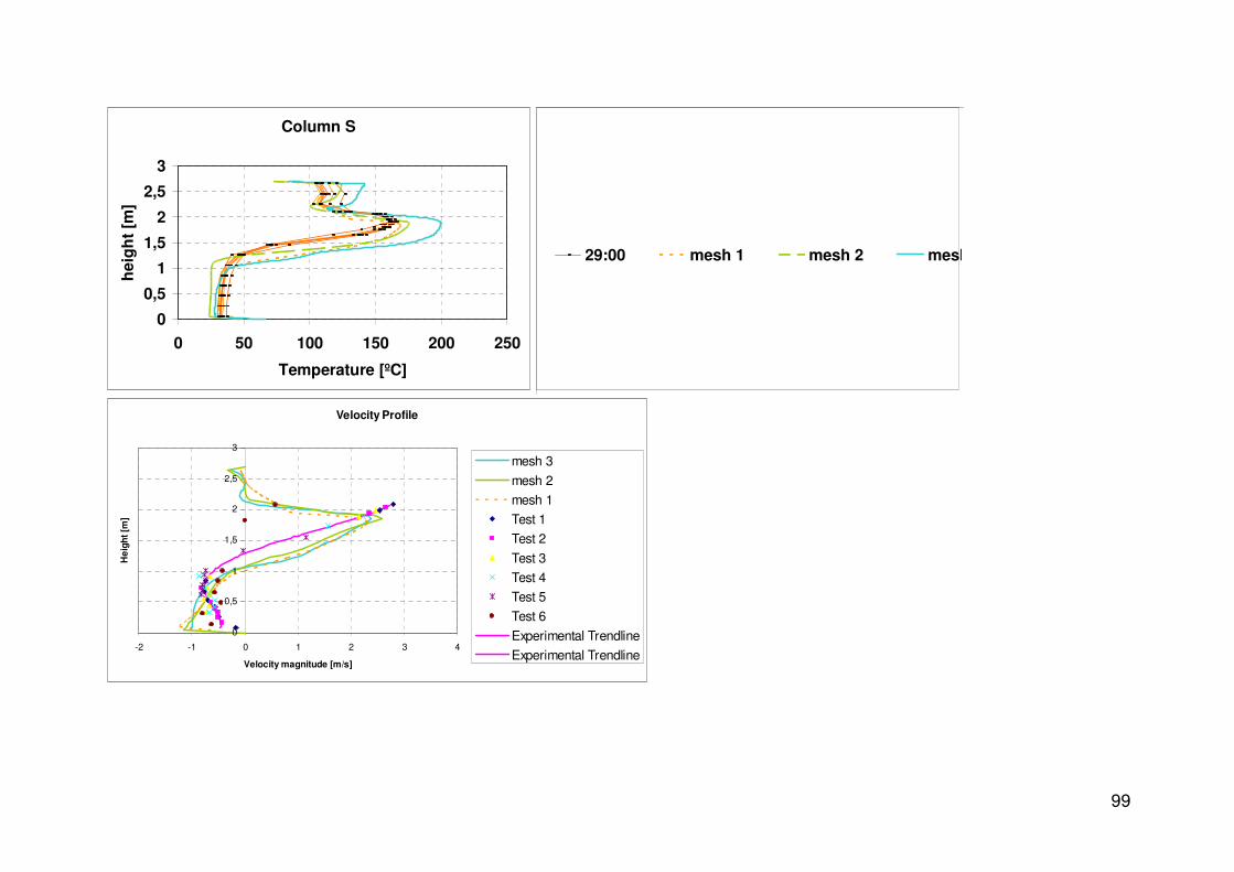
99
Column R
0
1
2
3
0 50 100 150 200 250
Temperature [ºC]
he
igh
t [m
]
29:00 mesh 1 mesh 2 mesh 3
Column S
0
0,5
1
1,5
2
2,5
3
0 50 100 150 200 250
Temperature [ºC]
heig
ht
[m]
Velocity Profile
0
0,5
1
1,5
2
2,5
3
-2 -1 0 1 2 3 4
Velocity magnitude [m/s]
He
igh
t [m
]
mesh 3
mesh 2
mesh 1
Test 1
Test 2
Test 3
Test 4
Test 5
Test 6
Experimental Trendline
Experimental Trendline

100
Appendix 12. Experimental Measurements at the old check in entrance
A B C D E
height [cm] Points A B C D E Porta
60 Velocity [m/s] 0,01 0,3 0,1 0,25 0,13
60 Temperature [ºC] 23,3 23,7 24 23,8 23,3
120 Velocity [m/s] 0,01 0,15 0,15 0,04 0 2,9
120 Temperature [ºC] 23,6 23,8 24,3 24,2 23,3 18,5
200 Velocity [m/s] 0,01 0,03 0,2 0,06 0,6
200 Temperature [ºC] 23,8 24,4 24,2 24,1 23,3

101
Appendix 13. LNEC Blueprints