Chandra News Issue 22Spring 2015

Published by the Chandra X-ray Center (CXC)

The Many Faces of Supernova Remnants

Tea Temim, Brian J. Williams, Laura Lopez

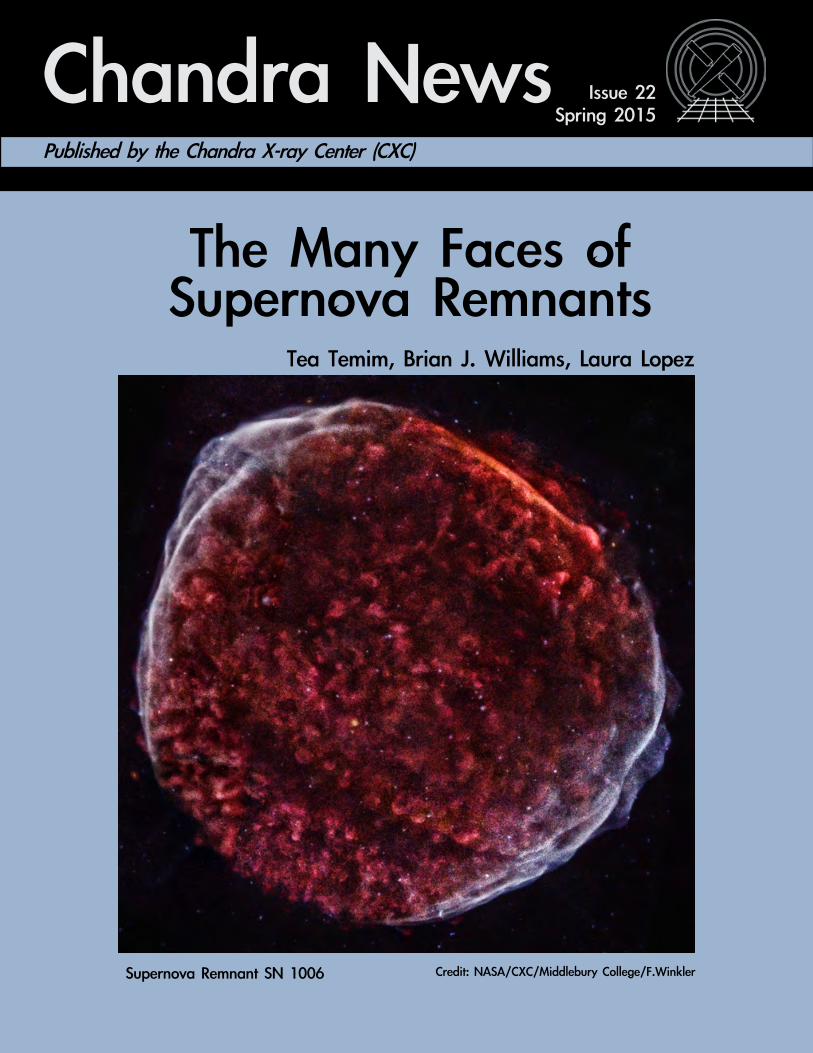
Supernova Remnant SN 1006 Credit: NASA/CXC/Middlebury College/F.Winkler

Contents

The Chandra Newsletter appears once a year and is authored by various CXC scientists, witheditorial assistance and layout by Evan Tingle. We welcome contributions from readers.

Comments on the newsletter, or corrections and additions to the hardcopy mailing list should be sent to: chandranews@cfa.harvard.edu.

Follow the Chandra Director's Office on Facebook, Google+ and Twitter (@ChandraCDO).

The Many Faces of Supernova RemnantsTea Temim, Brian J. Williams & Laura Lopez

Project Scientist’s ReportMartin Weisskopf

Project Manager’s ReportRoger Brissenden

Chandra Related Meetings and Important Dates

ACIS UpdatePaul Plucinsky, Royce Buehler, Gregg Germain & Richard Edgar

HRC UpdateRalph Kraft & Tomoki Kimura

HETGSMichael Nowak, for the HETGS Team

LETGJeremy J. Drake, for the LETG Team

Chandra CalibrationLarry P. David

Useful Web Addresses

15 Years of CIAOAntonella Fruscione, for the CIAO Team

Einstein Postdoctoral Fellowship ProgramPaul Green

Cycle 16 Peer Review ResultsAndrea Prestwich

Chandra Users’ Committee Membership List

CXC 2014 Science Press ReleasesMegan Watzke

‘‘15 Years of Science with Chandra’’ SymposiumDan Schwartz & Aneta Siemiginowska

24

27

30

26

31

18

37

41

42

43

16

15

22

3

12

13

14

21

Director's LogBelinda Wilkes

Chandra Source CatalogIan Evans, for the Chandra Source Catalog team

3Spring, 2015

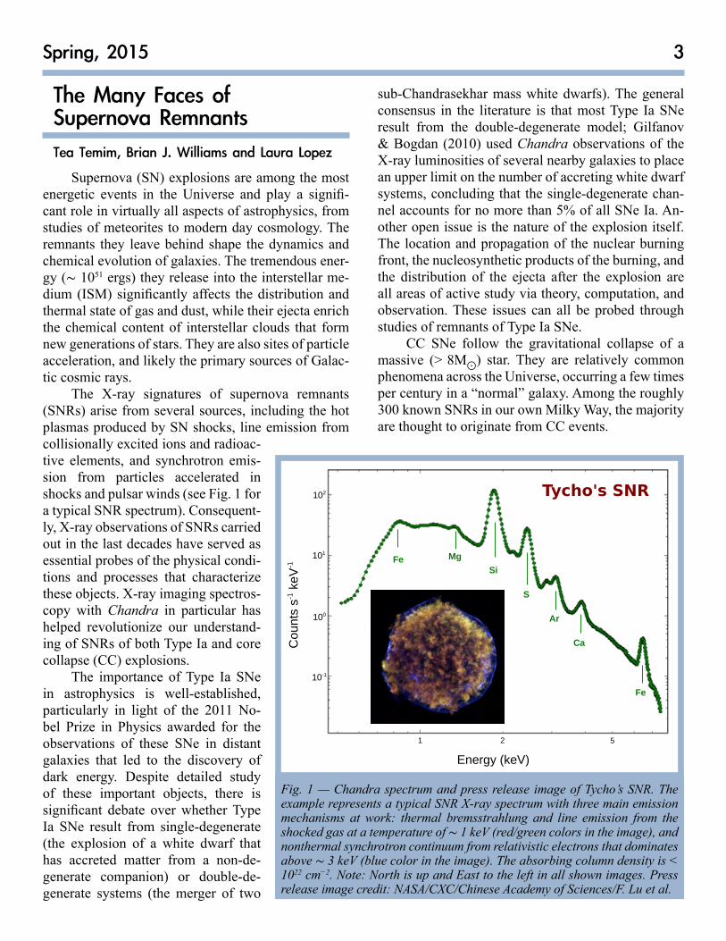
Fig. 1 — Chandra spectrum and press release image of Tycho’s SNR. The example represents a typical SNR X-ray spectrum with three main emission mechanisms at work: thermal bremsstrahlung and line emission from the shocked gas at a temperature of ∼ 1 keV (red/green colors in the image), and nonthermal synchrotron continuum from relativistic electrons that dominates above ∼ 3 keV (blue color in the image). The absorbing column density is < 1022 cm−2. Note: North is up and East to the left in all shown images. Press release image credit: NASA/CXC/Chinese Academy of Sciences/F. Lu et al.

The Many Faces of Supernova RemnantsTea Temim, Brian J. Williams and Laura Lopez

Supernova (SN) explosions are among the most energetic events in the Universe and play a signifi-cant role in virtually all aspects of astrophysics, from studies of meteorites to modern day cosmology. The remnants they leave behind shape the dynamics and chemical evolution of galaxies. The tremendous ener-gy (∼ 1051 ergs) they release into the interstellar me-dium (ISM) significantly affects the distribution and thermal state of gas and dust, while their ejecta enrich the chemical content of interstellar clouds that form new generations of stars. They are also sites of particle acceleration, and likely the primary sources of Galac-tic cosmic rays.

The X-ray signatures of supernova remnants (SNRs) arise from several sources, including the hot plasmas produced by SN shocks, line emission from collisionally excited ions and radioac-tive elements, and synchrotron emis-sion from particles accelerated in shocks and pulsar winds (see Fig. 1 for a typical SNR spectrum). Consequent-ly, X-ray observations of SNRs carried out in the last decades have served as essential probes of the physical condi-tions and processes that characterize these objects. X-ray imaging spectros-copy with Chandra in particular has helped revolutionize our understand-ing of SNRs of both Type Ia and core collapse (CC) explosions.

The importance of Type Ia SNe in astrophysics is well-established, particularly in light of the 2011 No-bel Prize in Physics awarded for the observations of these SNe in distant galaxies that led to the discovery of dark energy. Despite detailed study of these important objects, there is significant debate over whether Type Ia SNe result from single-degenerate (the explosion of a white dwarf that has accreted matter from a non-de-generate companion) or double-de-generate systems (the merger of two

sub-Chandrasekhar mass white dwarfs). The general consensus in the literature is that most Type Ia SNe result from the double-degenerate model; Gilfanov & Bogdan (2010) used Chandra observations of the X-ray luminosities of several nearby galaxies to place an upper limit on the number of accreting white dwarf systems, concluding that the single-degenerate chan-nel accounts for no more than 5% of all SNe Ia. An-other open issue is the nature of the explosion itself. The location and propagation of the nuclear burning front, the nucleosynthetic products of the burning, and the distribution of the ejecta after the explosion are all areas of active study via theory, computation, and observation. These issues can all be probed through studies of remnants of Type Ia SNe.

CC SNe follow the gravitational collapse of a massive (> 8M⨀) star. They are relatively common phenomena across the Universe, occurring a few times per century in a “normal” galaxy. Among the roughly 300 known SNRs in our own Milky Way, the majority are thought to originate from CC events.

1 2 5

Energy (keV)

Co

unts

s-1 k

eV

-1

Fe Mg

Si

S

Ar

Ca

Fe

Tycho's SNR

10-1

100

101

102

4 CXC Newsletter

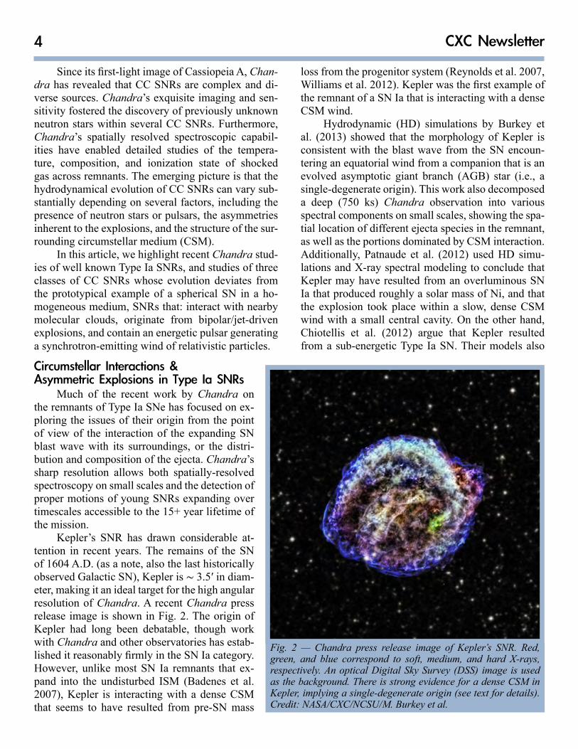
Fig. 2 — Chandra press release image of Kepler’s SNR. Red, green, and blue correspond to soft, medium, and hard X-rays, respectively. An optical Digital Sky Survey (DSS) image is used as the background. There is strong evidence for a dense CSM in Kepler, implying a single-degenerate origin (see text for details). Credit: NASA/CXC/NCSU/M. Burkey et al.

Since its first-light image of Cassiopeia A, Chan-dra has revealed that CC SNRs are complex and di-verse sources. Chandra’s exquisite imaging and sen-sitivity fostered the discovery of previously unknown neutron stars within several CC SNRs. Furthermore, Chandra’s spatially resolved spectroscopic capabil-ities have enabled detailed studies of the tempera-ture, composition, and ionization state of shocked gas across remnants. The emerging picture is that the hydrodynamical evolution of CC SNRs can vary sub-stantially depending on several factors, including the presence of neutron stars or pulsars, the asymmetries inherent to the explosions, and the structure of the sur-rounding circumstellar medium (CSM).

In this article, we highlight recent Chandra stud-ies of well known Type Ia SNRs, and studies of three classes of CC SNRs whose evolution deviates from the prototypical example of a spherical SN in a ho-mogeneous medium, SNRs that: interact with nearby molecular clouds, originate from bipolar/jet-driven explosions, and contain an energetic pulsar generating a synchrotron-emitting wind of relativistic particles.

Circumstellar Interactions & Asymmetric Explosions in Type Ia SNRs

Much of the recent work by Chandra on the remnants of Type Ia SNe has focused on ex-ploring the issues of their origin from the point of view of the interaction of the expanding SN blast wave with its surroundings, or the distri-bution and composition of the ejecta. Chandra’s sharp resolution allows both spatially-resolved spectroscopy on small scales and the detection of proper motions of young SNRs expanding over timescales accessible to the 15+ year lifetime of the mission.

Kepler’s SNR has drawn considerable at-tention in recent years. The remains of the SN of 1604 A.D. (as a note, also the last historically observed Galactic SN), Kepler is ∼ 3.5′ in diam-eter, making it an ideal target for the high angular resolution of Chandra. A recent Chandra press release image is shown in Fig. 2. The origin of Kepler had long been debatable, though work with Chandra and other observatories has estab-lished it reasonably firmly in the SN Ia category. However, unlike most SN Ia remnants that ex-pand into the undisturbed ISM (Badenes et al. 2007), Kepler is interacting with a dense CSM that seems to have resulted from pre-SN mass

loss from the progenitor system (Reynolds et al. 2007, Williams et al. 2012). Kepler was the first example of the remnant of a SN Ia that is interacting with a dense CSM wind.

Hydrodynamic (HD) simulations by Burkey et al. (2013) showed that the morphology of Kepler is consistent with the blast wave from the SN encoun-tering an equatorial wind from a companion that is an evolved asymptotic giant branch (AGB) star (i.e., a single-degenerate origin). This work also decomposed a deep (750 ks) Chandra observation into various spectral components on small scales, showing the spa-tial location of different ejecta species in the remnant, as well as the portions dominated by CSM interaction. Additionally, Patnaude et al. (2012) used HD simu-lations and X-ray spectral modeling to conclude that Kepler may have resulted from an overluminous SN Ia that produced roughly a solar mass of Ni, and that the explosion took place within a slow, dense CSM wind with a small central cavity. On the other hand, Chiotellis et al. (2012) argue that Kepler resulted from a sub-energetic Type Ia SN. Their models also

5Spring, 2015

require the presence of a dense CSM, generated by the winds from a symbiotic binary consisting of a white dwarf and an AGB companion. Clearly, Kepler and Kepler-like SNRs are deserving of more study to de-termine their origins.

The remnant of SN 1006 A.D. provides some-thing of a contrast to Kepler. There, the densities are extremely low with no indication of a CSM, making a double-degenerate progenitor system seem more like-ly. Perhaps the most Chandra-centric result from SN 1006 is a study of the proper motions of the forward shock, which moves at a rate of roughly one Chandra pixel per year. Fig. 3 shows a difference image in two epochs (2003 and 2012) of Chandra observations of SN 1006 (Winkler et al. 2014). Expansion along the NE and SW limbs, where the emission is dominated by non-thermal synchrotron X-rays, is readily appar-ent, as the shocks there move at 5000–6000 km s−1. The ISM density is somewhat higher in the NW, where X-rays are dominated by thermal emission from the shocked ISM. Proper motions there are less apparent but still visible. The shock speed there is significantly slower, moving at ∼ 3000 km s−1 (Katsuda et al. 2013). That SN 1006 is still approximately circular, despite such variations in the expansion rate, indicates that the blast wave’s interaction with the denser material in the NW is a relatively recent phenomenon. Winkler et al. (2013) estimate that this interaction began about 150 years ago.

Perhaps the most interesting new result on SN 1006 is the discovery that the ejecta distribution is asymmetric. Equivalent width image maps of the various atomic species present in the thermal X-ray plasma can map out the distribution of these elements within the remnant. Chandra maps from Winkler et al. (2014) and Suzaku maps from Uchida et al. (2013) both show that Si and Fe, primarily originating from the reverse-shocked ejecta, are more prevalent in the SE portion of SN 1006. O and Ne, on the other hand, which likely originate from the forward-shocked ISM, are more uniformly distributed. HD models of SNe Ia can show asymmetries in the ejecta related to the par-ticulars of the explosion; see, for example, Seitenzahl et al. (2013).

Further evidence for an asymmetric explosion of a (likely) SN Ia is found in G1.9+0.3, the youngest known remnant in the Galaxy at an age of about 150 years. The young age of this remnant was first dis-covered by Reynolds et al. (2008), who compared a newly obtained Chandra image to an archival radio

image from two decades prior, noting that the rem-nant had expanded by roughly 20% during that time. In G1.9+0.3, the intermediate mass elements Si and S, byproducts of O-burning, have a different spatial distribution than Fe (Borkowski et al. 2013). Ejecta velocities in this remnant are observed to be > 18,000 km s−1, which may imply an energetic Type Ia event. The expansion velocities of the forward and reverse shocks in G1.9+0.3 also show significant variation by factors of ∼ 60% in different places in the remnant (Borkowski et al. 2014), again indicating an asymmet-ric explosion.

Chandra observations of Tycho’s SNR, the rem-nant of the SN of 1572 A.D., show remarkable differ-ences when viewed in soft and hard X-rays. At lower energies, below ∼ 2 keV, the X-ray emission is domi-nated by thermal emission from the ejecta, mostly Si, in a somewhat fluffy morphology (see Fig. 1). At hard X-ray energies, emission is dominated by nonthermal synchrotron photons, mostly coming from the forward shock. However, in the western portion, a curious pat-tern emerges of stripes emanating radially outwards. This pattern has not yet been seen in any other rem-nant. Eriksen et al. (2011) argue that these stripes are

Fig. 3 — Difference image between the 2003 and 2012 Chandra observations of SN 1006, showing expansion of the remnant during that time period (Fig. 6 from Winkler et al. 2014). Expansion is particularly evident along the synchrotron-dominated NE and SW limbs, where shock speeds are 5000 –6000 km s -1. Image is approximately 40′ on a side.

6 CXC Newsletter

regions of unusually high magnetic field turbulence, and their roughly constant spacing corresponds to the gyroradii of 1014 −1015 eV protons. If this interpreta-tion is correct, it would be evidence of the acceler-ation of protons by SNR shocks, long thought to be the source of most Galactic cosmic rays, at least up to energies of around 1015 eV.

Shocked Clouds & Enriching Jets in Core-Collapse SNRs

Since the progenitors of CC SNe have short main-sequence lives, the explosions tend to occur within the dense medium from which the massive stars were born. Consequently, a common trait of CC SNRs is interaction with an inhomogeneous or dense CSM. In fact, roughly one quarter of all Galactic SNRs show evidence of interaction with molecular clouds, such as the coincidence of OH masers (which indicate the presence of shocked molecular gas: e.g., Wardle & Yusef-Zadeh 2002).

The SNR-molecular cloud interaction has a pro-found influence on the X-ray morphologies and spec-tra of the SNRs. Large-scale density gradients can re-sult in substantial deviations from spherical symmetry (e.g., Lopez et al. 2009). Additionally, a large number of interacting SNRs have centrally dominated, ther-mal X-ray emission, whereas their radio morphologies are shell-like. Known as mixed morphology (MM) SNRs, ∼ 40 of these sources have been identified in the Milky Way (Vink 2012). Based on observations with Chandra and other modern X-ray facilities, MM SNRs can have enhanced metal abundances (Lazendic

& Slane 2006) and/or isothermal plasmas across their interiors.

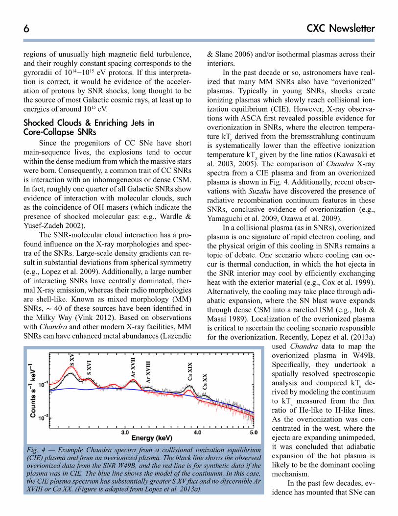
In the past decade or so, astronomers have real-ized that many MM SNRs also have “overionized” plasmas. Typically in young SNRs, shocks create ionizing plasmas which slowly reach collisional ion-ization equilibrium (CIE). However, X-ray observa-tions with ASCA first revealed possible evidence for overionization in SNRs, where the electron tempera-ture kTe derived from the bremsstrahlung continuum is systematically lower than the effective ionization temperature kTz given by the line ratios (Kawasaki et al. 2003, 2005). The comparison of Chandra X-ray spectra from a CIE plasma and from an overionized plasma is shown in Fig. 4. Additionally, recent obser-vations with Suzaku have discovered the presence of radiative recombination continuum features in these SNRs, conclusive evidence of overionization (e.g., Yamaguchi et al. 2009, Ozawa et al. 2009).

In a collisional plasma (as in SNRs), overionized plasma is one signature of rapid electron cooling, and the physical origin of this cooling in SNRs remains a topic of debate. One scenario where cooling can oc-cur is thermal conduction, in which the hot ejecta in the SNR interior may cool by efficiently exchanging heat with the exterior material (e.g., Cox et al. 1999). Alternatively, the cooling may take place through adi-abatic expansion, where the SN blast wave expands through dense CSM into a rarefied ISM (e.g., Itoh & Masai 1989). Localization of the overionized plasma is critical to ascertain the cooling scenario responsible for the overionization. Recently, Lopez et al. (2013a)

used Chandra data to map the overionized plasma in W49B. Specifically, they undertook a spatially resolved spectroscopic analysis and compared kTe de-rived by modeling the continuum to kTz measured from the flux ratio of He-like to H-like lines. As the overionization was con-centrated in the west, where the ejecta are expanding unimpeded, it was concluded that adiabatic expansion of the hot plasma is likely to be the dominant cooling mechanism.

In the past few decades, ev-idence has mounted that SNe can

Fig. 4 — Example Chandra spectra from a collisional ionization equilibrium (CIE) plasma and from an overionized plasma. The black line shows the observed overionized data from the SNR W49B, and the red line is for synthetic data if the plasma was in CIE. The blue line shows the model of the continuum. In this case, the CIE plasma spectrum has substantially greater S XV flux and no discernible Ar XVIII or Ca XX. (Figure is adapted from Lopez et al. 2013a).

7Spring, 2015

have significant deviations from spherical symmetry. In particular, spectropolarimetry studies demonstrate that both Type Ia and CC SNe are aspherical near maximum brightness (e.g., Wang & Wheeler 2008). SNRs retain imprints of the geometry of their progen-itors’ explosions, and spectro-imaging studies with Chandra have revealed marked asymmetries in young SNRs, such as the silicon-rich “jet” in Cassiopeia A which protrudes from the remnant’s forward shock (Hughes et al. 2000). The analysis of the morphology of the Chandra X-ray line emission in Galactic and Large Magellanic Cloud SNRs established that CC SNRs are statistically more asymmetric and elliptical than Type Ia SNRs (Lopez et al. 2009, 2011). Infra-red observations of SNRs were later shown to display these same properties (Peters et al. 2013).

Asymmetric explosions also alter the nucleosyn-thetic yields of the SNe (e.g., Maeda & Nomoto 2003). For example, while spherical CC events are predicted to produce ∼ 0.07– 0.15 M⨀ of 56Ni, bipolar/jet-driv-en CC SNe (with increased kinetic energy at the poles of exploding stars) can have 5–10 times more nickel (Umeda & Nomoto 2008).

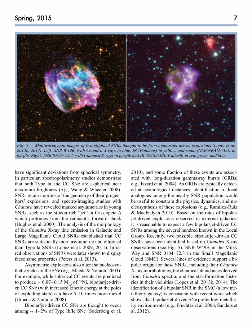
Bipolar/jet-driven CC SNe are thought to occur among ∼ 1– 2% of Type Ib/Ic SNe (Soderberg et al.

2010), and some fraction of these events are associ-ated with long-duration gamma-ray bursts (GRBs; e.g., Izzard et al. 2004). As GRBs are typically detect-ed at cosmological distances, identification of local analogues among the nearby SNR population would be useful to constrain the physics, dynamics, and nu-cleosynthesis of these explosions (e.g., Ramirez-Ruiz & MacFadyen 2010). Based on the rates of bipolar/jet-driven explosions observed in external galaxies, it is reasonable to expect a few bipolar/jet-driven CC SNRs among the several hundred known in the Local Group. Recently, two possible bipolar/jet-driven CC SNRs have been identified based on Chandra X-ray observations (see Fig. 5): SNR W49B in the Milky Way and SNR 0104−72.3 in the Small Magellanic Cloud (SMC). Several lines of evidence support a bi-polar origin for these SNRs, including their Chandra X-ray morphologies, the chemical abundances derived from Chandra spectra, and the star-formation histo-ries in their vicinities (Lopez et al. 2013b, 2014). The identification of a bipolar SNR in the SMC (a low me-tallicity galaxy) is consistent with recent work which shows that bipolar/jet-driven SNe prefer low-metallic-ity environments (e.g., Fruchter et al. 2006, Sanders et al. 2012).

Fig. 5 — Mulitwavelength images of two elliptical SNRs thought to be from bipolar/jet-driven explosions (Lopez et al. 2013b, 2014). Left: SNR W49B, with Chandra X-rays in blue, IR (Palomar) in yellow, and radio (NSF/NRAO/VLA) in purple. Right: SNR 0104−72.3, with Chandra X-rays in purple and IR (NASA/JPL-Caltech) in red, green, and blue.

8 CXC Newsletter

Fleeing Pulsars & Crushed Winds in Composite SNRs

Composite SNRs are a special subclass of CC remnants that are not only characterized by forward and reverse shocks that expand into the ambient medi-um and the cold SN ejecta, but also a highly magnetic, rapidly rotating pulsar that converts its spin-down en-ergy into a wind of relativistic particles. The acceler-ation of these particles in the pulsar’s magnetic field produces a synchrotron-emitting pulsar wind nebula (PWN) that retains a torus and jet morphology im-printed by the rotating magnetic field. In composite SNRs, the evolution of the PWN is coupled to the evo-lution of its host SNR. The complex interaction that occurs allows us to probe the properties of the pulsar, the SN ejecta, the progenitor star, and the structure of the ambient medium. It also alters the relativistic par-ticle population that eventually escapes into the ISM, and gives rise to an excess of low-energy particles that produce γ-ray emission through inverse-Compton scattering (e.g., Abdo et al. 2012, Slane et al. 2010). For these reasons, the study of the composite class of SNRs has been of particular interest.

Chandra observations of composite SNRs in var-ious stages of evolution significantly advanced our un-derstanding of these systems. While the basic picture of their evolution was generally understood, Chandra filled in the crucial details pertaining to the transitional phases of evolution. High-resolution imaging provided unprecedentedly detailed views of the structures that form in each stage of development, from the well-de-fined tori and jets in younger system to highly disrupt-ed nebulae in older ones. Spectral studies revealed the spatially varying spectra of the evolving particle popu-lation injected by the pulsar, and provided evidence for the mixing of SN ejecta with PWN material. Here, we highlight only a selection of studies of the PWN/SNR interaction conducted with Chandra in recent years.

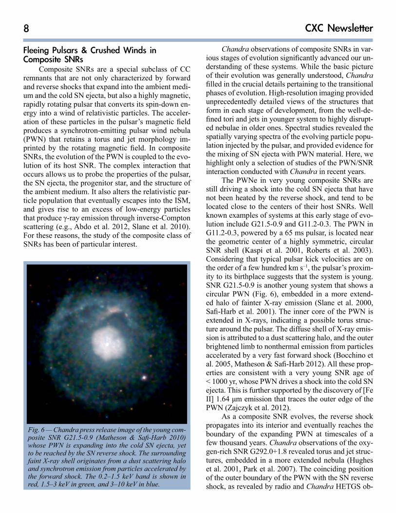
The PWNe in very young composite SNRs are still driving a shock into the cold SN ejecta that have not been heated by the reverse shock, and tend to be located close to the centers of their host SNRs. Well known examples of systems at this early stage of evo-lution include G21.5-0.9 and G11.2-0.3. The PWN in G11.2-0.3, powered by a 65 ms pulsar, is located near the geometric center of a highly symmetric, circular SNR shell (Kaspi et al. 2001, Roberts et al. 2003). Considering that typical pulsar kick velocities are on the order of a few hundred km s−1, the pulsar’s proxim-ity to its birthplace suggests that the system is young. SNR G21.5-0.9 is another young system that shows a circular PWN (Fig. 6), embedded in a more extend-ed halo of fainter X-ray emission (Slane et al. 2000, Safi-Harb et al. 2001). The inner core of the PWN is extended in X-rays, indicating a possible torus struc-ture around the pulsar. The diffuse shell of X-ray emis-sion is attributed to a dust scattering halo, and the outer brightened limb to nonthermal emission from particles accelerated by a very fast forward shock (Bocchino et al. 2005, Matheson & Safi-Harb 2012). All these prop-erties are consistent with a very young SNR age of < 1000 yr, whose PWN drives a shock into the cold SN ejecta. This is further supported by the discovery of [Fe II] 1.64 μm emission that traces the outer edge of the PWN (Zajczyk et al. 2012).

As a composite SNR evolves, the reverse shock propagates into its interior and eventually reaches the boundary of the expanding PWN at timescales of a few thousand years. Chandra observations of the oxy-gen-rich SNR G292.0+1.8 revealed torus and jet struc-tures, embedded in a more extended nebula (Hughes et al. 2001, Park et al. 2007). The coinciding position of the outer boundary of the PWN with the SN reverse shock, as revealed by radio and Chandra HETGS ob-

Fig. 6 — Chandra press release image of the young com-posite SNR G21.5-0.9 (Matheson & Safi-Harb 2010) whose PWN is expanding into the cold SN ejecta, yet to be reached by the SN reverse shock. The surrounding faint X-ray shell originates from a dust scattering halo and synchrotron emission from particles accelerated by the forward shock. The 0.2–1.5 keV band is shown in red, 1.5–3 keV in green, and 3–10 keV in blue.

9Spring, 2015

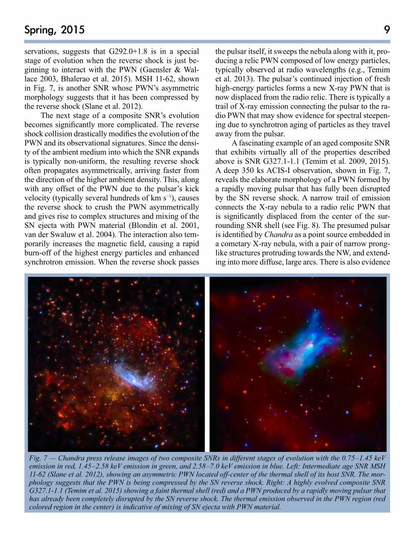
servations, suggests that G292.0+1.8 is in a special stage of evolution when the reverse shock is just be-ginning to interact with the PWN (Gaensler & Wal-lace 2003, Bhalerao et al. 2015). MSH 11-62, shown in Fig. 7, is another SNR whose PWN’s asymmetric morphology suggests that it has been compressed by the reverse shock (Slane et al. 2012).

The next stage of a composite SNR’s evolution becomes significantly more complicated. The reverse shock collision drastically modifies the evolution of the PWN and its observational signatures. Since the densi-ty of the ambient medium into which the SNR expands is typically non-uniform, the resulting reverse shock often propagates asymmetrically, arriving faster from the direction of the higher ambient density. This, along with any offset of the PWN due to the pulsar’s kick velocity (typically several hundreds of km s−1), causes the reverse shock to crush the PWN asymmetrically and gives rise to complex structures and mixing of the SN ejecta with PWN material (Blondin et al. 2001, van der Swaluw et al. 2004). The interaction also tem-porarily increases the magnetic field, causing a rapid burn-off of the highest energy particles and enhanced synchrotron emission. When the reverse shock passes

Fig. 7 — Chandra press release images of two composite SNRs in different stages of evolution with the 0.75 –1.45 keV emission in red, 1.45 –2.58 keV emission in green, and 2.58 –7.0 keV emission in blue. Left: Intermediate age SNR MSH 11-62 (Slane et al. 2012), showing an asymmetric PWN located off-center of the thermal shell of its host SNR. The mor-phology suggests that the PWN is being compressed by the SN reverse shock. Right: A highly evolved composite SNR G327.1-1.1 (Temim et al. 2015) showing a faint thermal shell (red) and a PWN produced by a rapidly moving pulsar that has already been completely disrupted by the SN reverse shock. The thermal emission observed in the PWN region (red colored region in the center) is indicative of mixing of SN ejecta with PWN material.

the pulsar itself, it sweeps the nebula along with it, pro-ducing a relic PWN composed of low energy particles, typically observed at radio wavelengths (e.g., Temim et al. 2013). The pulsar’s continued injection of fresh high-energy particles forms a new X-ray PWN that is now displaced from the radio relic. There is typically a trail of X-ray emission connecting the pulsar to the ra-dio PWN that may show evidence for spectral steepen-ing due to synchrotron aging of particles as they travel away from the pulsar.

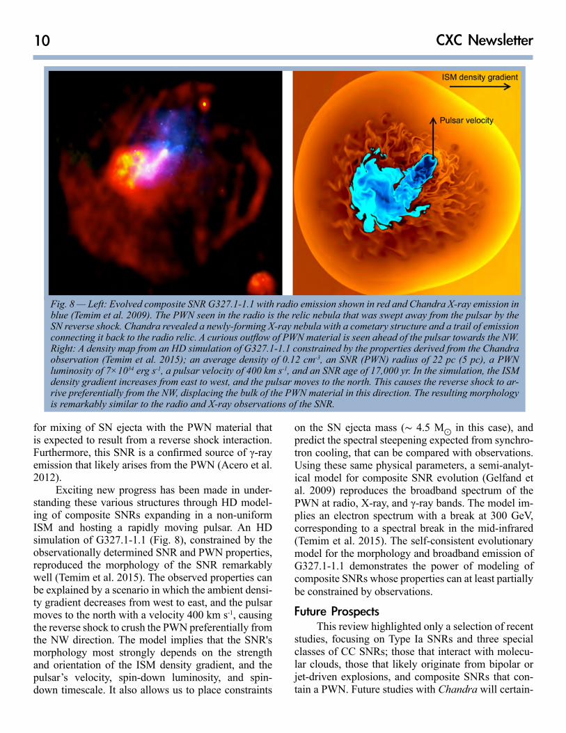
A fascinating example of an aged composite SNR that exhibits virtually all of the properties described above is SNR G327.1-1.1 (Temim et al. 2009, 2015). A deep 350 ks ACIS-I observation, shown in Fig. 7, reveals the elaborate morphology of a PWN formed by a rapidly moving pulsar that has fully been disrupted by the SN reverse shock. A narrow trail of emission connects the X-ray nebula to a radio relic PWN that is significantly displaced from the center of the sur-rounding SNR shell (see Fig. 8). The presumed pulsar is identified by Chandra as a point source embedded in a cometary X-ray nebula, with a pair of narrow prong-like structures protruding towards the NW, and extend-ing into more diffuse, large arcs. There is also evidence

10 CXC Newsletter

for mixing of SN ejecta with the PWN material that is expected to result from a reverse shock interaction. Furthermore, this SNR is a confirmed source of γ-ray emission that likely arises from the PWN (Acero et al. 2012).

Exciting new progress has been made in under-standing these various structures through HD model-ing of composite SNRs expanding in a non-uniform ISM and hosting a rapidly moving pulsar. An HD simulation of G327.1-1.1 (Fig. 8), constrained by the observationally determined SNR and PWN properties, reproduced the morphology of the SNR remarkably well (Temim et al. 2015). The observed properties can be explained by a scenario in which the ambient densi-ty gradient decreases from west to east, and the pulsar moves to the north with a velocity 400 km s-1, causing the reverse shock to crush the PWN preferentially from the NW direction. The model implies that the SNR's morphology most strongly depends on the strength and orientation of the ISM density gradient, and the pulsar’s velocity, spin-down luminosity, and spin-down timescale. It also allows us to place constraints

on the SN ejecta mass (∼ 4.5 M⨀ in this case), and predict the spectral steepening expected from synchro-tron cooling, that can be compared with observations. Using these same physical parameters, a semi-analyt-ical model for composite SNR evolution (Gelfand et al. 2009) reproduces the broadband spectrum of the PWN at radio, X-ray, and γ-ray bands. The model im-plies an electron spectrum with a break at 300 GeV, corresponding to a spectral break in the mid-infrared (Temim et al. 2015). The self-consistent evolutionary model for the morphology and broadband emission of G327.1-1.1 demonstrates the power of modeling of composite SNRs whose properties can at least partially be constrained by observations.

Future ProspectsThis review highlighted only a selection of recent

studies, focusing on Type Ia SNRs and three special classes of CC SNRs; those that interact with molecu-lar clouds, those that likely originate from bipolar or jet-driven explosions, and composite SNRs that con-tain a PWN. Future studies with Chandra will certain-

Fig. 8 — Left: Evolved composite SNR G327.1-1.1 with radio emission shown in red and Chandra X-ray emission in blue (Temim et al. 2009). The PWN seen in the radio is the relic nebula that was swept away from the pulsar by the SN reverse shock. Chandra revealed a newly-forming X-ray nebula with a cometary structure and a trail of emission connecting it back to the radio relic. A curious outflow of PWN material is seen ahead of the pulsar towards the NW. Right: A density map from an HD simulation of G327.1-1.1 constrained by the properties derived from the Chandra observation (Temim et al. 2015); an average density of 0.12 cm-3, an SNR (PWN) radius of 22 pc (5 pc), a PWN luminosity of 7×1034 erg s-1, a pulsar velocity of 400 km s-1, and an SNR age of 17,000 yr. In the simulation, the ISM density gradient increases from east to west, and the pulsar moves to the north. This causes the reverse shock to ar-rive preferentially from the NW, displacing the bulk of the PWN material in this direction. The resulting morphology is remarkably similar to the radio and X-ray observations of the SNR.

11Spring, 2015

ly further increase our knowledge about these systems and provide insight into many of the outstanding ques-tions.

Chandra will potentially identify other prospects for Type Ia SNRs that have CSM interactions, particu-larly in coordination with HD simulations. Its longev-ity has a serendipitous effect in that the baseline for proper motion studies only grows longer. Older mea-surements can be refined and new expansion measure-ments can be made for the first time, even for more distant SNRs.

Chandra and XMM-Newton will be necessary to spatially resolve the overionized plasma and ascertain the cause of the rapid electron cooling in interacting SNRs. Future kinematic studies can confirm the bipo-lar nature of some SNRs, as it is predicted that heavy metals (Cr, Mn, Fe) should have faster velocities than lighter elements (O, Mg, Si). Additionally, improved measurements of chemical abundances via X-ray spec-troscopy may better constrain parameters like the pro-genitor mass, the explosion energy, and the jet opening angle.

Future modeling of composite SNRs in different evolutionary stages promises to further improve our understanding of the PWN/SNR interaction, constrain parameters such as the pulsar’s spin-down timescale and the SN ejecta mass, and help uncover the eventual fate of accelerated particles that escape into the ISM. The models will hinge on high-resolution observation-al studies with Chandra that can constrain the PWN structure, spatial variations in the PWN spectrum, and the properties of the SNR thermal emission.

The fifteen years of Chandra observations have led to extraordinary advances in our understanding of the evolution of SNRs and the origin of their diversity. The next fifteen years hold the promise of many more great discoveries.

Acknowledgments The authors thank Pat Slane for providing in-

sightful comments on the article.

ReferencesAcero, F., Djannati-Ataï, A., Förster, A., et al. 2012, arX-iv:1201.0481.Abdo, A. A., Ackermann, M., Ajello, M., et al. 2010, ApJ, 713, 146.Badenes, C., et al. 2007, ApJ, 662, 472.Bhalerao, J., Park, S., Dewey, D., et al. 2015, ApJ, 800, 65.Blondin, J. M., Chevalier, R. A., & Frierson, D. M. 2001, ApJ, 563, 806.Bocchino, F., van der Swaluw, E., Chevalier, R., & Band-

iera, R. 2005, A&A, 442, 539Borkowski, K. J., et al. 2013, ApJ, 771, 9.Borkowski, K. J., et al. 2014, ApJ, 790, 18.Burkey, M. T., et al. 2013, ApJ, 764, 63.Chiotellis, A., et al. 2012, A&A, 537, 139.Cox, D. P, et al. 1999, ApJ, 524, 179.Eriksen, K. A., et al. 2011, ApJ, 728, 28.Fruchter, A. S., et al. 2006, Nature, 441, 463.Gaensler, B. M., & Wallace, B. J. 2003, ApJ, 594, 326.Gilfanov, M. & Bogdan, A. 2010, Nature, 463, 924.Hughes, J. P., et al. 2000, ApJL, 528, L109.Hughes, J. P., Slane, P. O., Burrows, D. N., et al. 2001, ApJL, 559, L153.Itoh, H. & Masai, K. 1989, MNRAS, 236, 885.Izzard, R. G., et al. 2004, MNRAS, 348, 1215.Kawasaki, M. et al. 2005, ApJ, 631, 935.Kaspi, V. M., Roberts, M. E., Vasisht, G., et al. 2001, ApJ, 560, 371.Katsuda, S., et al. 2013, ApJ, 763, 85.Matheson, H., & Safi-Harb, S. 2010, ApJ, 724, 572.Lopez, L., et al. 2009, ApJ, 706, 106.Lopez, L., et al. 2011, ApJ, 732, 114.Lopez, L., et al. 2013a, ApJ, 777, 145.Lopez, L., et al. 2013b, ApJ, 764, 50.Lopez, L., et al. 2014, ApJ, 777, 5.Maeda, K. & Nomoto, K. 2003, ApJ, 598, 1163.Ozawa, M. et al. 2009, ApJL, 706, L71.Park, S., Hughes, J. P., Slane, P. O., et al. 2007, ApJ, 670, L121.Patnaude, D. J., et al. 2012, ApJ, 756, 6.Peters et al. 2013, ApJL, 771, L38.Ramirez-Ruiz & MacFadyen 2010, ApJ, 716, 1028.Reynolds, S.P., et al. 2007, ApJ, 668, 135.Reynolds, S.P., et al. 2008, ApJ, 680, 41.Roberts, M. S. E., Tam, C. R., Kaspi, V. M., et al. 2003, ApJ, 588, 992.Safi-Harb, S., Harrus, I. M., Petre, R., et al. 2001, ApJ, 561, 308.Sanders, N. E., et al. 2012, ApJ, 758, 132.Seitenzahl, I. R., et al. 2013, MNRAS, 429, 1156.Soderberg, A., et al. 2010, Nature, 463, 513.Slane, P., Castro, D., Funk, S., et al. 2010, ApJ, 720, 266.Slane, P., Chen, Y., Schulz, N. S., et al. 2000, ApJ, 533, L29.Slane, P., Hughes, J. P., Temim, T., et al. 2012, ApJ, 749, 131.Temim, T., Slane, P., Castro, D., et al. 2013, ApJ, 768, 61.Temim, T., Slane, P., Gaensler, B. M., Hughes, J. P., & Van Der Swaluw, E. 2009, ApJ, 691, 895.Temim, T, et al. 2015, ApJ, submitted.Uchida, H., et al. 2013, ApJ, 771, 56.van der Swaluw, E., Downes, T. P., & Keegan, R. 2004, A&A, 420, 937.Vink, J. 2012, A&AR, 20, 49.Wang, L. & Wheeler, C. J. 2008, ARA&A, 46, 433.Wardle, M. & Yusef-Zadeh, F. 2002, Science, 296, 2350.Williams, B.J., et al. 2012, ApJ, 755, 3.

12 CXC Newsletter

Director’s LogChandra Date: 550108804

Belinda Wilkes

It is now a year since my transition to Director of the Chandra X-ray Center on 20 April 2014, follow-ing founding Director, Dr. Harvey Tananbaum’s retire-ment (http://chandra.harvard.edu/press/14_releases/press_031914.html). During this past year, I have vis-ited our various local sites as well as the MSFC Proj-ect Office and NASA HQ, and have met with manag-ers, team leads, and many individual staff. I have very much enjoyed getting to know the team in more depth. The more I learn, the more impressed I am by the tal-ent, professionalism, dedication, in-depth knowledge, and sheer hard work of all the members of the Chan-dra team, many of whom have been with the Program since well before launch.

A number of exciting events have taken place in the past year. Chandra celebrated 15 years of ground-breaking science in 2014! Our talented Pub-lic Communications team arranged a number of on-line and live events, including a press release to mark the launch anniversary (http://chandra.harvard.edu/press/14_releases/press_072214.html). Cake and ice cream were consumed to celebrate other key anniver-saries: e.g., launch on 23 July, first light on 19 Aug, along with many reminiscences and well-deserved pats-on-the-back.

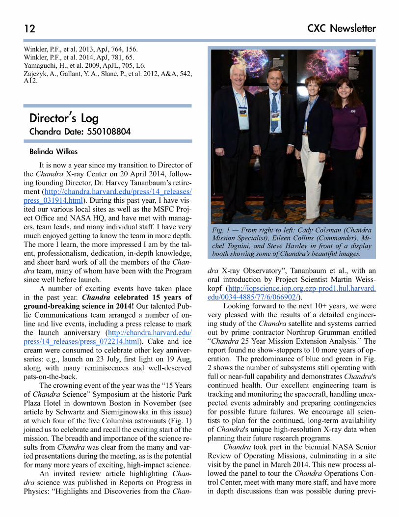
The crowning event of the year was the “15 Years of Chandra Science” Symposium at the historic Park Plaza Hotel in downtown Boston in November (see article by Schwartz and Siemiginowska in this issue) at which four of the five Columbia astronauts (Fig. 1) joined us to celebrate and recall the exciting start of the mission. The breadth and importance of the science re-sults from Chandra was clear from the many and var-ied presentations during the meeting, as is the potential for many more years of exciting, high-impact science.

An invited review article highlighting Chan-dra science was published in Reports on Progress in Physics: “Highlights and Discoveries from the Chan-

Fig. 1 — From right to left: Cady Coleman (Chandra Mission Specialist), Eileen Collins (Commander), Mi-chel Tognini, and Steve Hawley in front of a display booth showing some of Chandra’s beautiful images.

Winkler, P.F., et al. 2013, ApJ, 764, 156.Winkler, P.F., et al. 2014, ApJ, 781, 65.Yamaguchi, H., et al. 2009, ApJL, 705, L6.Zajczyk, A., Gallant, Y. A., Slane, P., et al. 2012, A&A, 542, A12.

dra X-ray Observatory”, Tananbaum et al., with an oral introduction by Project Scientist Martin Weiss-kopf (http://iopscience.iop.org.ezp-prod1.hul.harvard.edu/0034-4885/77/6/066902/).

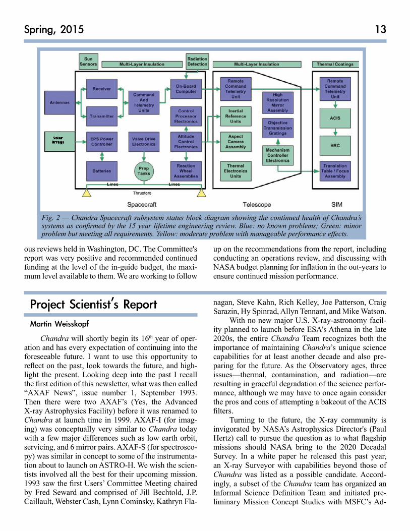
Looking forward to the next 10+ years, we were very pleased with the results of a detailed engineer-ing study of the Chandra satellite and systems carried out by prime contractor Northrop Grumman entitled “Chandra 25 Year Mission Extension Analysis.” The report found no show-stoppers to 10 more years of op-eration. The predominance of blue and green in Fig. 2 shows the number of subsystems still operating with full or near-full capability and demonstrates Chandra's continued health. Our excellent engineering team is tracking and monitoring the spacecraft, handling unex-pected events admirably and preparing contingencies for possible future failures. We encourage all scien-tists to plan for the continued, long-term availability of Chandra's unique high-resolution X-ray data when planning their future research programs.

Chandra took part in the biennial NASA Senior Review of Operating Missions, culminating in a site visit by the panel in March 2014. This new process al-lowed the panel to tour the Chandra Operations Con-trol Center, meet with many more staff, and have more in depth discussions than was possible during previ-

13Spring, 2015

Fig. 2 — Chandra Spacecraft subsystem status block diagram showing the continued health of Chandra’s systems as confirmed by the 15 year lifetime engineering review. Blue: no known problems; Green: minor problem but meeting all requirements. Yellow: moderate problem with manageable performance effects.

ous reviews held in Washington, DC. The Committee's report was very positive and recommended continued funding at the level of the in-guide budget, the maxi-mum level available to them. We are working to follow

up on the recommendations from the report, including conducting an operations review, and discussing with NASA budget planning for inflation in the out-years to ensure continued mission performance.

Project Scientist’s ReportMartin Weisskopf

Chandra will shortly begin its 16th year of oper-ation and has every expectation of continuing into the foreseeable future. I want to use this opportunity to reflect on the past, look towards the future, and high-light the present. Looking deep into the past I recall the first edition of this newsletter, what was then called “AXAF News”, issue number 1, September 1993. Then there were two AXAF’s (Yes, the Advanced X-ray Astrophysics Facility) before it was renamed to Chandra at launch time in 1999. AXAF-I (for imag-ing) was conceptually very similar to Chandra today with a few major differences such as low earth orbit, servicing, and 6 mirror pairs. AXAF-S (for spectrosco-py) was similar in concept to some of the instrumenta-tion about to launch on ASTRO-H. We wish the scien-tists involved all the best for their upcoming mission. 1993 saw the first Users’ Committee Meeting chaired by Fred Seward and comprised of Jill Bechtold, J.P. Caillault, Webster Cash, Lynn Cominsky, Kathryn Fla-

nagan, Steve Kahn, Rich Kelley, Joe Patterson, Craig Sarazin, Hy Spinrad, Allyn Tennant, and Mike Watson.

With no new major U.S. X-ray-astronomy facil-ity planned to launch before ESA's Athena in the late 2020s, the entire Chandra Team recognizes both the importance of maintaining Chandra’s unique science capabilities for at least another decade and also pre-paring for the future. As the Observatory ages, three issues—thermal, contamination, and radiation—are resulting in graceful degradation of the science perfor-mance, although we may have to once again consider the pros and cons of attempting a bakeout of the ACIS filters.

Turning to the future, the X-ray community is invigorated by NASA’s Astrophysics Director's (Paul Hertz) call to pursue the question as to what flagship missions should NASA bring to the 2020 Decadal Survey. In a white paper he released this past year, an X-ray Surveyor with capabilities beyond those of Chandra was listed as a possible candidate. Accord-ingly, a subset of the Chandra team has organized an Informal Science Definition Team and initiated pre-liminary Mission Concept Studies with MSFC’s Ad-

14 CXC Newsletter

vanced Concepts Office to provide input over the next several months to the Physics of the Cosmos Program Advisory Group in support of such a mission. We en-visage this facility to have angular resolution at least as good as Chandra, and effective area of about 2.5 square meters with ∼ 1 arcsec resolution over a 5 arc-min × 5 arcmin field of view. We trust that those mem-bers of the community that especially feel the impact of the number of detected photons on their research will rally around this concept.

I would like to close by mentioning a new Chan-dra/HST result that is soon to be published in Science: “The Non-Gravitational Interactions of Dark Matter in Colliding Galaxy Clusters” by D. Harvey, R. Massey, T. Kitching, A. Taylor, and E. Tittley. Not only does this work, which blends results from Chandra and HST, show the awesome synergy that derives from NASA’s Great Observatory Program, but it also leads us deeper into the mysterious physics of the Dark Matter, which pervades the Universe.

Project Manager’s ReportRoger Brissenden

Chandra has marked over 15 years of success-ful mission operations with continued excellent op-erational and scientific performance. Telescope time remained in high demand, with significant oversub-scription in the Cycle 16 peer review, held in June 2014. The Cycle 16 review approved 190 proposals, out of 634 submitted by researchers worldwide who requested 108 Msec of observing time, ∼ 4.8 times greater than the time available. Among the approved proposals are three X-ray Visionary Projects (XVPs), which were allocated a total of 5.4 Msec. XVPs are longer observing programs intended to address major questions in astrophysics and to produce data sets of lasting value.

In the Fall, the observing program transitioned from Cycle 15 to Cycle 16. Due to the gradual evo-lution of Chandra’s orbit, which has reduced the nonproductive time spent in Earth’s radiation belts, Chandra’s overall observing efficiency has general-ly been near the highest level of the mission, result-ing in higher than average allocated observing time. However, with continued orbit evolution the available time will slowly decrease in future years. We released the Call for Proposals for Cycle 17 in December, with

proposals due in March 2015 and the peer review in June 2015.

In response to NASA’s request for proposals for the 2014 Senior Review of operating missions, Chan-dra X-ray Center (CXC) and Marshall Space Flight Center program staff submitted the Chandra propos-al January 2014. The NASA review committee held a site visit at the CXC in March. In their final report, the committee recognized Chandra’s capabilities and sci-entific productivity, saying “The prospects for further compelling science return in the future are excellent. This panel enthusiastically endorses the extension of the Chandra mission….The staff and infrastructure of the Chandra Project are most effective at enabling new science….Chandra discoveries continue to have an extraordinarily high impact on both the scientific and public understanding of our universe.” The com-mittee recommended that “mission operations and the ground system should be examined by senior engi-neers from other NASA projects for new ideas that may result in cost efficiencies.” The CXC will host an operations review for this purpose in May 2015.

In October, the CXC hosted the annual sympo-sium for the Einstein Fellowship program. A CXC workshop, “The X-ray View of Galaxy Ecosystems,” originally planned for the summer of 2013 but can-celled due to NASA restrictions on conferences and travel, was held in July 2014. As part of the CXC’s regular reviews and consultations with outside orga-nizations, NASA reviewed the CXC’s operations in April and October, and the Chandra Users’ Commit-tee met at the CXC in October.

After several years of very low solar radiation, the sun has become more active, resulting in Chan-dra observing being interrupted three times during the year to protect the instruments from solar particles. In addition, seven requests to observe targets of opportu-nity required the mission planning and flight teams to interrupt and revise on-board command loads. Chan-dra passed through the 2014 spring and fall eclipse seasons with nominal power and thermal performance.

In May of 2014, Chandra encountered a new meteor shower, the Camelopardalids, when the Earth crossed the path of comet 209P/LINEAR. To prepare for this passage, the CXC flight team developed and implemented procedures to point the observatory in the anti-radiant direction and partially feather the solar arrays to reduce their cross section. Chandra passed the shower successfully, with no known damage.

Engineers from the flight team and other experts completed a detailed review of Chandra’s systems to

15Spring, 2015

Chandra Related Meetings and Important Dates

Cycle 17 Peer Review: June 22–26, 2015

Cycle 17 Cost Proposals Due: September 17, 2015

X-ray Spectra Workshop: August 19-21, 2015

Users’ Committee Meeting: Late Sept./Early Oct., 2015

Einstein Fellows Symposium: October 27-28, 2015

Cycle 17 Start: December, 2015

Cycle 18 Call for Proposals: December, 2015

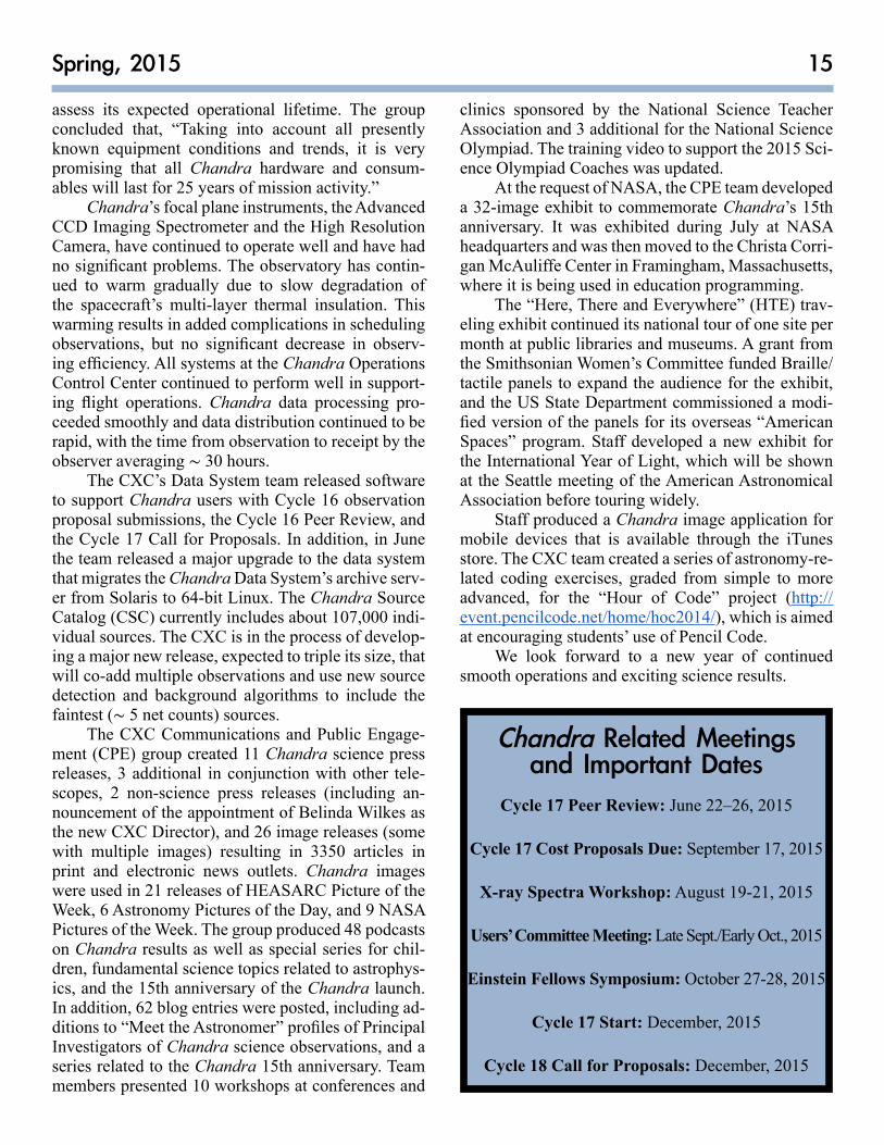
assess its expected operational lifetime. The group concluded that, “Taking into account all presently known equipment conditions and trends, it is very promising that all Chandra hardware and consum-ables will last for 25 years of mission activity.”

Chandra’s focal plane instruments, the Advanced CCD Imaging Spectrometer and the High Resolution Camera, have continued to operate well and have had no significant problems. The observatory has contin-ued to warm gradually due to slow degradation of the spacecraft’s multi-layer thermal insulation. This warming results in added complications in scheduling observations, but no significant decrease in observ-ing efficiency. All systems at the Chandra Operations Control Center continued to perform well in support-ing flight operations. Chandra data processing pro-ceeded smoothly and data distribution continued to be rapid, with the time from observation to receipt by the observer averaging ∼ 30 hours.

The CXC’s Data System team released software to support Chandra users with Cycle 16 observation proposal submissions, the Cycle 16 Peer Review, and the Cycle 17 Call for Proposals. In addition, in June the team released a major upgrade to the data system that migrates the Chandra Data System’s archive serv-er from Solaris to 64-bit Linux. The Chandra Source Catalog (CSC) currently includes about 107,000 indi-vidual sources. The CXC is in the process of develop-ing a major new release, expected to triple its size, that will co-add multiple observations and use new source detection and background algorithms to include the faintest (∼ 5 net counts) sources.

The CXC Communications and Public Engage-ment (CPE) group created 11 Chandra science press releases, 3 additional in conjunction with other tele-scopes, 2 non-science press releases (including an-nouncement of the appointment of Belinda Wilkes as the new CXC Director), and 26 image releases (some with multiple images) resulting in 3350 articles in print and electronic news outlets. Chandra images were used in 21 releases of HEASARC Picture of the Week, 6 Astronomy Pictures of the Day, and 9 NASA Pictures of the Week. The group produced 48 podcasts on Chandra results as well as special series for chil-dren, fundamental science topics related to astrophys-ics, and the 15th anniversary of the Chandra launch. In addition, 62 blog entries were posted, including ad-ditions to “Meet the Astronomer” profiles of Principal Investigators of Chandra science observations, and a series related to the Chandra 15th anniversary. Team members presented 10 workshops at conferences and

clinics sponsored by the National Science Teacher Association and 3 additional for the National Science Olympiad. The training video to support the 2015 Sci-ence Olympiad Coaches was updated.

At the request of NASA, the CPE team developed a 32-image exhibit to commemorate Chandra’s 15th anniversary. It was exhibited during July at NASA headquarters and was then moved to the Christa Corri-gan McAuliffe Center in Framingham, Massachusetts, where it is being used in education programming.

The “Here, There and Everywhere” (HTE) trav-eling exhibit continued its national tour of one site per month at public libraries and museums. A grant from the Smithsonian Women’s Committee funded Braille/tactile panels to expand the audience for the exhibit, and the US State Department commissioned a modi-fied version of the panels for its overseas “American Spaces” program. Staff developed a new exhibit for the International Year of Light, which will be shown at the Seattle meeting of the American Astronomical Association before touring widely.

Staff produced a Chandra image application for mobile devices that is available through the iTunes store. The CXC team created a series of astronomy-re-lated coding exercises, graded from simple to more advanced, for the “Hour of Code” project (http://event.pencilcode.net/home/hoc2014/), which is aimed at encouraging students’ use of Pencil Code.

We look forward to a new year of continued smooth operations and exciting science results.

16 CXC Newsletter

‘‘15 Years of Science with Chandra’’ SymposiumDan Schwartz and Aneta Siemiginowska

July 23, 2014 marked the 15 year anniversary of the launch of the Chandra X-ray Observatory. A Sym-posium was held in Boston Park Plaza on November 18-21, 2014 celebrating the key science results from the recent years of Chandra operations. Topics and themes emphasized the high-resolution imaging and spectroscopy which is only possible with Chandra, including theory and related data from other observa-tories.

The Symposium was attended by more than 150 scientists including 12 invited speakers: Victoria Kaspi, Jacco Vink, David Huenemoerder, Giuseppi-na Fabbiano, Antara Basu-Zych, Francesca Civano, Julie Hlavacek-Larrondo, Brad Benson, Giuseppina Micela, Rodolfo Montez, Daryl Haggard, and Jon Miller. Their excellent review talks together with the contributions from other participants spanned a broad range of science topics, from the sun to stars to distant galaxies, clusters of galaxies and quasars, underly-ing the importance of Chandra and its unprecedented high angular resolution mirrors. Posters remained up throughout the week, with dedicated breaks (with re-freshments) encouraging lively interactions.

Paul Hertz commented on “The past, present and future role of X-ray astronomy at NASA” and pro-vided information about the upcoming opportunities and the timeline for the 2020 Decadal Survey. Alexey Vikhlinin presented a concept for an X-ray Sur-veyor mission, SMART-X (http://smart-x.cfa.harvard.edu/), a high-throughput X-ray observa-tory with Chandra-like angular resolution which utilizes new technologies for adjustable, light-weight mirrors and a new generation of science instruments. SMART-X would be the true suc-cessor to Chandra, and could be realized in the 2020s. Chandra remains robust to any credible single point failure, with many new discoveries to come during the remaining 10+ years of ex-pected lifetime.

The Symposium included a Special Session on future science with Chandra and discussion of the high priority science objectives identified by the Science Panels in the New World, New Horizons Decadal study. The panel discussion was led by the CXC Director Belinda Wilkes and

included the New World, New Horizon’s panel chairs and members: Roger Chevalier, Daniel Wang, Meg Urry, David Weinberg, and Eric Feigelson. Each pan-elist gave a short presentation highlighting the topic of their Decadal panel. All agreed that the Chandra capabilities are unique and could support many of the key science goals identified in the Decadal study.

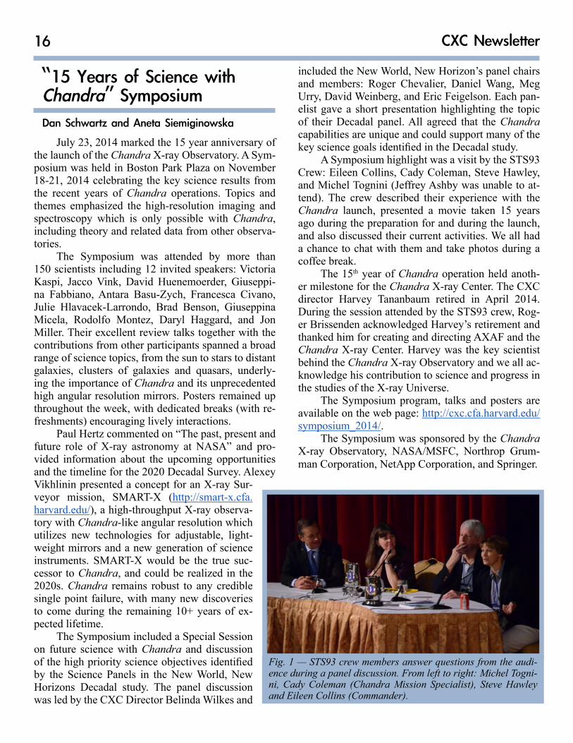
A Symposium highlight was a visit by the STS93 Crew: Eileen Collins, Cady Coleman, Steve Hawley, and Michel Tognini (Jeffrey Ashby was unable to at-tend). The crew described their experience with the Chandra launch, presented a movie taken 15 years ago during the preparation for and during the launch, and also discussed their current activities. We all had a chance to chat with them and take photos during a coffee break.

The 15th year of Chandra operation held anoth-er milestone for the Chandra X-ray Center. The CXC director Harvey Tananbaum retired in April 2014. During the session attended by the STS93 crew, Rog-er Brissenden acknowledged Harvey’s retirement and thanked him for creating and directing AXAF and the Chandra X-ray Center. Harvey was the key scientist behind the Chandra X-ray Observatory and we all ac-knowledge his contribution to science and progress in the studies of the X-ray Universe.

The Symposium program, talks and posters are available on the web page: http://cxc.cfa.harvard.edu/symposium_2014/.

The Symposium was sponsored by the Chandra X-ray Observatory, NASA/MSFC, Northrop Grum-man Corporation, NetApp Corporation, and Springer.

Fig. 1 — STS93 crew members answer questions from the audi-ence during a panel discussion. From left to right: Michel Togni-ni, Cady Coleman (Chandra Mission Specialist), Steve Hawley and Eileen Collins (Commander).

17Spring, 2015

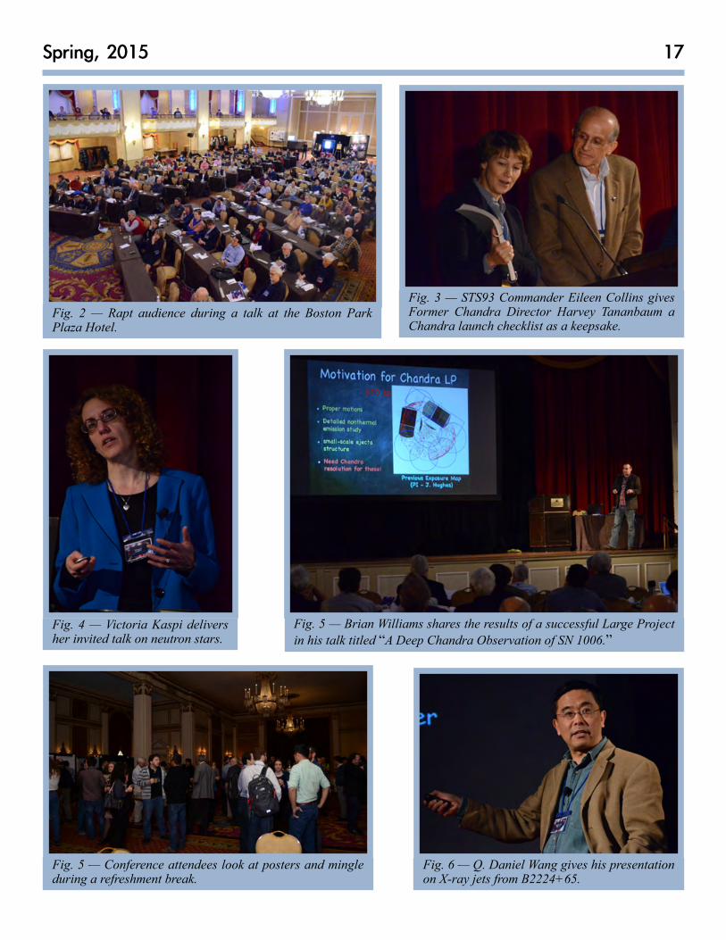
Fig. 3 — STS93 Commander Eileen Collins gives Former Chandra Director Harvey Tananbaum a Chandra launch checklist as a keepsake.

Fig. 2 — Rapt audience during a talk at the Boston Park Plaza Hotel.

Fig. 6 — Q. Daniel Wang gives his presentation on X-ray jets from B2224+65.

Fig. 5 — Conference attendees look at posters and mingle during a refreshment break.

Fig. 4 — Victoria Kaspi delivers her invited talk on neutron stars.

Fig. 5 — Brian Williams shares the results of a successful Large Project in his talk titled “A Deep Chandra Observation of SN 1006.”

18 CXC Newsletter

Chandra Source CatalogIan Evans, for the Chandra Source Catalog team

The current release of the Chandra Source Cat-alog (CSC) continues to be well utilized by the as-tronomical community. Usage over the past year has averaged more than 10,000 searches per month, summed across the various user and virtual observa-tory catalog interfaces supported by the CXC. Ver-sion 1.1 of the CSC, released in late 2010, includes properties and data for 158,071 detections from 5,110 Chandra observations, comprising 106,586 distinct sources on the sky.

When we released version 1.1 of the CSC, our plan was to provide an updated version of the cat-alog once sufficient new data had been accumu-lated. However, during the period since release 1.1, the CSC team at the CXC has received numer-ous suggestions from the community for improve-

ments to be included in release 2.0 of the catalog, and we have carefully considered how to best respond to those requests. The most common request for release 2.0 was to “go deeper”, and that is where our efforts have been concentrated. Release 2.0 will not only go deeper, but will also include 5 more years of data (ob-servations released publicly during 2010–2014) than the previous release.

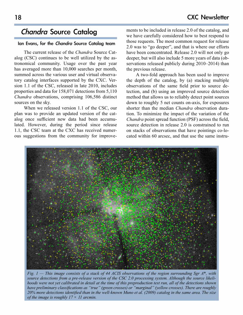
A two-fold approach has been used to improve the depth of the catalog, by (a) stacking multiple observations of the same field prior to source de-tection, and (b) using an improved source detection method that allows us to reliably detect point sources down to roughly 5 net counts on-axis, for exposures shorter than the median Chandra observation dura-tion. To minimize the impact of the variation of the Chandra point spread function (PSF) across the field, source detection in release 2.0 is constrained to run on stacks of observations that have pointings co-lo-cated within 60 arcsec, and that use the same instru-

1.5 1.6 1.8 2.2 3 4.5 7.6 14 26 51 1e+02Fig. 1 — This image consists of a stack of 44 ACIS observations of the region surrounding Sgr A*, with source detections from a pre-release version of the CSC 2.0 processing system. Although the source likeli-hoods were not yet calibrated in detail at the time of this preproduction test run, all of the detections shown have preliminary classifications as “true” (green crosses) or “marginal” (yellow crosses). There are roughly 20% more detections identified than in the well-known Muno et al. (2009) catalog in the same area. The size of the image is roughly 17 × 11 arcmin.

19Spring, 2015

ment. Source detection is performed primarily using the CIAO wavelet detection tool (wavdetect) that was used for release 1.1, but with the tool parame-ters updated to detect fainter candidate sources, albe-it with an unacceptably large false detection rate. A new maximum likelihood estimator, mle, uses Sher-pa to fit the local PSF model (and with the local PSF model convolved with an elliptical Gaussian, to sim-ulate sources with inherent extent) to each candidate source, in order to evaluate the likelihood that the candidate source is real. Candidate source detections will be classified as either “true” or “marginal” in the catalog, depending on their likelihood. However, cat-alog users will be able to access the lists of all candi-date source detections regardless of these thresholds. Fitting with the local PSF should also improve source astrometry, particularly for larger off-axis angles where PSF asymmetries can bias the wavdetect po-sition determinations.

Release 2.0 uses a new Voronoi-tessellation background tool, mkvtbkg, to create improved back-ground maps prior to source detection. In many cases, these background maps perform better than the release 1.1 maps in regions where the background intensity is changing rapidly, for example near galaxy cores, and at large off-axis angles. As a side effect, mkvtbkg can identify regions containing extended emission, and this capability will be used to include bright, extend-ed sources in the CSC for the first time. Such sourc-es will include a bounding convex hull polygon in the catalog. Sets of polygons with multiple intensity thresholds will be available to end users who wish to perform more detailed analyses of detected extended sources. The impact of better backgrounds, stacking observations, and deeper detections using the wav-detect/mle combination is demonstrated spectacu-larly in Figs. 1 and 2, from a preproduction test run of the catalog pipeline on the Sgr A* field.

1.5 1.6 1.7 2 2.6 3.8 6.1 11 20 38 75

18

36

20

85

14114

67

362

12

34

11

4331

33

47

31

7

7

20

15

50

8

16

10

73

10

1516

11

15

13

56

19

12

23

26

30

22

44

12

30

32

20

18

9

10

12

22

52

28

2594

14

16

21

42

39

40

24

17

18

27

11

20

12

100

28

47

44

14

17

23

28

15

30

15

42

48

15

54

14

28

59

25

31

22

130

24

16

35

13

30

33

30

42

28

27

23

24

29

22

40

41

30

16

38

135

37

31

32

22

33

43

90

38

52

40

61

43

22

30

83129

26

61

39

56

17

34

47

129

26

31

73

47

42

45

47

40

53

60

58

30

39

55

113

83

184

277138

44

47

66

84

54

196

35

33

65

6878

103

76

138

165

103

113

310

255

235

257

130

341

1603

1044

1498

372

Fig. 2 — This image zooms in on a region of the field to the South of the core of Sgr A*. The green and yellow crosses indicate the fitted source positions for “true” and “marginal” sources respec-tively, with error ellipses shown in most cases (error ellipses were not generated in all cases in this preproduction test run). The numbers listed with the detections are the raw (i.e., uncalibrated) source likelihood values. The red circles show the source positions from the Muno et al. (2009) cata-log. A number of sources not present in the Muno et al. catalog are visible in the stacked images, and are detected in the CSC 2.0 preproduction test run. Conversely, a small number of sources reported in the Muno et al. catalog are not detected (or are below threshold) in the test run. Some differences in detections are to be expected at the faint limit, since the dataset used herein includes ∼ 1/3 more exposure than the dataset of Muno et al. The size of the image is roughly 128 × 80 arcsec.

20 CXC Newsletter

Enhancements to the Bayesian aperture photom-etry code are included in release 2.0 of the CSC, and the photometric probability density functions are used directly for computing such quantities as hardness ra-tios and temporal variability measures, to avoid some inconsistencies present in release 1.1 of the catalog where these properties were computed independently.

Sources detected at the edges of the field of view, in the gaps between ACIS back-illuminated and front-illuminated chips (on the ACIS-S array), and on readout streaks associated with saturated, bright sources, are excluded from the CSC 2.0. In release 1.1, a significant fraction of sources in these regions were determined to be false. Release 2.0 will include limiting sensitivity maps computed on a fine-grained (4 × 4 arcsec) scale so that users can identify regions that are included in/excluded from the catalog.

As in release 1.1, CSC 2.0 will include numerous raw measurements for each detected source, as well as scientifically useful properties (and associated er-rors) derived from the observations in which a source is located. These properties include estimates of the source position, extent, and aperture photometry flux-es in several energy bands. Cross-band spectral hard-ness ratios will be reported for all detected sources, together with absorbed power-law, bremsstrahlung, and black-body spectral fits for brighter sources. Several source variability measures will be comput-ed, both within a single observation of a source and between multiple observations that include the same source.

In addition to the tabulated properties, CSC 2.0 will provide FITS (and in some cases, JPEG) for-mat data products that include full field event lists, multi-band images, exposure maps, limiting sensitiv-ity maps, merged source lists, and extended source polygons. Source region data products include per-source-region event lists, multi-band images, pho-tometry probability density functions, exposure maps, pulse-invariant spectra, spectral response matrices, and optimally binned light curves.

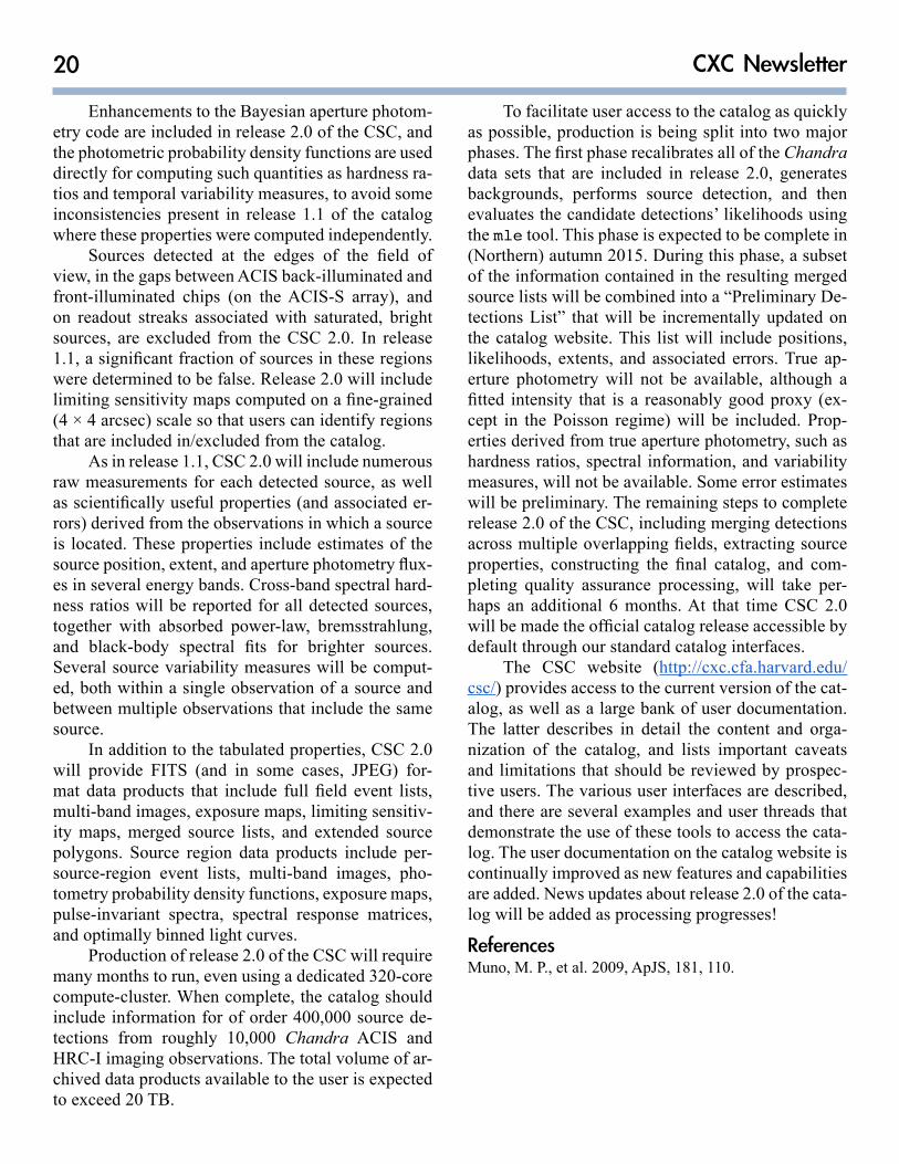
Production of release 2.0 of the CSC will require many months to run, even using a dedicated 320-core compute-cluster. When complete, the catalog should include information for of order 400,000 source de-tections from roughly 10,000 Chandra ACIS and HRC-I imaging observations. The total volume of ar-chived data products available to the user is expected to exceed 20 TB.

To facilitate user access to the catalog as quickly as possible, production is being split into two major phases. The first phase recalibrates all of the Chandra data sets that are included in release 2.0, generates backgrounds, performs source detection, and then evaluates the candidate detections’ likelihoods using the mle tool. This phase is expected to be complete in (Northern) autumn 2015. During this phase, a subset of the information contained in the resulting merged source lists will be combined into a “Preliminary De-tections List” that will be incrementally updated on the catalog website. This list will include positions, likelihoods, extents, and associated errors. True ap-erture photometry will not be available, although a fitted intensity that is a reasonably good proxy (ex-cept in the Poisson regime) will be included. Prop-erties derived from true aperture photometry, such as hardness ratios, spectral information, and variability measures, will not be available. Some error estimates will be preliminary. The remaining steps to complete release 2.0 of the CSC, including merging detections across multiple overlapping fields, extracting source properties, constructing the final catalog, and com-pleting quality assurance processing, will take per-haps an additional 6 months. At that time CSC 2.0 will be made the official catalog release accessible by default through our standard catalog interfaces.

The CSC website (http://cxc.cfa.harvard.edu/csc/) provides access to the current version of the cat-alog, as well as a large bank of user documentation. The latter describes in detail the content and orga-nization of the catalog, and lists important caveats and limitations that should be reviewed by prospec-tive users. The various user interfaces are described, and there are several examples and user threads that demonstrate the use of these tools to access the cata-log. The user documentation on the catalog website is continually improved as new features and capabilities are added. News updates about release 2.0 of the cata-log will be added as processing progresses!

ReferencesMuno, M. P., et al. 2009, ApJS, 181, 110.

21Spring, 2015

ACIS UpdatePaul Plucinsky, Royce Buehler, Gregg Germain, and Richard Edgar

The ACIS instrument continued to perform well over the past year conducting the vast majority of GO observations with Chandra. There were only a few interruptions to the scheduled observations due to anomalies with the ACIS instrument. The most seri-ous of these was the unexpected power off of the side A of the Digital Processing Assembly (DPA) on 11 January 2015. Side A of the DPA had spontaneously turned off on two occasions earlier in the mission. For each of those occurrences, the most likely explana-tion for the anomaly was a single event upset (SEU) that resulted in a spurious power off command to the electronics. An examination of the telemetry from the January 2015 event showed that this anomaly was consistent with the previous anomalies. Based on this conclusion, the ACIS instrument team prepared real-time command procedures to restore the ACIS instru-ment to its nominal configuration to conduct science observations. The recovery to the nominal configura-tion was completed 18.5 hours after the anomaly was detected and science observations resumed soon af-terward. Side A of the DPA has functioned nominally since the recovery.

The charge-transfer inefficiency (CTI) of the FI and BI CCDs is increasing at the expected rate. The contamination layer continues to accumulate on the ACIS optical-blocking filter. A new calibration file (labelled N0009) to model the absorption due to the contamination layer was released by the CXC calibra-tion group in the 4.6.2 release of the Chandra Cali-bration Database (CALDB) on 9 July 2014. This cali-bration file significantly improves the accuracy of the model for data acquired after mid-2013. If GOs are analyzing data since that time and the response at low energies is important for their analysis, they should be using the contamination model in CALDB 4.6.2 or later. Analysis of calibration observations of 1E0102-7219 in March 2015 show that the N0009 contamina-tion model is still accurately predicting the growth of the contamination layer near the aimpoints on the S3 and I3 CCDs. However, these observations indicate that the contamination layer might be growing faster near the bottom and top edges of the S3 CCD. This preliminary result will need to be confirmed with cal-

ibration observations of other sources. Observations of A1795 are in the schedule for April 2015. GOs who have analyses sensitive to the low energy response at the top and bottom of the S3 CCD should monitor the CXC calibration web pages for future updates to the contamination file.

The control of the ACIS focal plane (FP) tem-perature continues to be a major focus of the ACIS Operations Team. As the Chandra thermal environ-ment continues to evolve over the mission, some of the components in the Science Instrument Module (SIM) close to ACIS have been reaching higher tem-peratures, making it more difficult to maintain the de-sired -119.7 °C at the focal plane. GOs can increase the probability that the FP temperature will be cold and stable for their observation by reducing the num-ber of operational CCDs, which reduces the power dissipation in the FP, thereby resulting in a lower FP temperature. GOs can select CCDs that are “required” or “optional” for their observation. Starting in Cycle 16, GOs were encouraged to select 4 or fewer required CCDs for their observations to keep the FP and the electronics cooler, if their science objectives can be met with that arrangement. Starting in Cycle 14, GOs were not allowed to select “Y” for 6 CCDs in the RPS forms when they submit their proposal. If a GO re-quires 6 CCDs for their observation, they are to select 5 CCDs as “Y” and one CCD as “OFF1” at the time of proposal submission. If the proposal is selected, the GO may work with their User Uplink Support Scien-tist and change the “OFF1” to a “Y” if the sixth CCD is required. GOs are still allowed to select 5 CCDs as required when they submit their proposals. GOs should be aware that requesting 6 CCDs increases the likelihood of a warm FP temperature and/or may in-crease the complexity of scheduling the observation. GOs should review the updated material in the Pro-posers’ Observatory Guide on selecting CCDs.

GOs who are new to ACIS are encouraged to read the Proposers’ Guide and the help pages on the RPS form on selecting an energy filter. The RPS forms request two quantities: the “Lower Energy Threshold” and the “Energy Filter Range.” The first parameter sets the minimum energy an event must have to be select-ed for inclusion in the telemetry. The second param-eter sets the range of energies starting from the lower energy threshold that are to be included. For example, if the lower energy threshold is set to 0.3 keV and the energy filter range is set to 12.0 keV, ACIS will select

22 CXC Newsletter

events with energies between 0.3 and 12.3 keV for inclusion in the telemetry. GOs should be advised that the onboard estimate of the energy of an event is not as accurate as the estimate after the data have been processed on the ground. Therefore it is wise to select an energy range that is slightly broader to be more in-clusive such that events are included in telemetry and then a more restrictive filter may be applied by the GO when they analyze their data. The only exception to this is if the energy filter is needed to reduce the count rate to prevent telemetry saturation. In such cases, the GO might want to be more restrictive with the energy filter.

ACIS allows the GO to set two energy filters. The first filter discussed above applies to all events from all CCDs. In addition, ACIS also allows the GO to specify another energy filter in a spatial win-dow. For example, a GO could specify a lower en-ergy threshold of 0.3 keV and an energy filter range of 12.0 keV for all CCDs and specify another energy filter with a lower energy threshold of 1.0 keV and an energy filter range of 5.0 keV. ACIS would only accept events with energies between 1.0 and 6.0 keV inside the region defined by the spatial window but it would accept events with energies between 0.3 keV and 12.3 keV for all regions outside of the spatial re-gion. But GOs should be careful since the energy fil-ters are combined as a logical “AND.” The candidate X-ray event must satisfy both filters in order to be ac-cepted, therefore the filters should be consistent with each other to provide the energies that the GO desires. In the example above, the global energy filter accepts events between 0.3 keV and 12.3 keV and the energy filter in the spatial window accepts events with ener-gies between 1.0 and 6.0 keV. Therefore, the energy filter in the spatial window will reject events if the energy is between 0.3 and 1.0 keV and if the energy is between 6.0 and 12.3 keV. If a GO were to specify a global energy filter with a lower energy threshold of 0.3 keV and an energy filter range of 12.0 keV and an energy filter in the spatial window with a lower energy threshold of 1.0 keV and an energy filter range of 12.0 keV, the events with energies between 12.3 keV and 13.0 keV in the region defined by the spatial window would not be accepted into telemetry because their energies are outside of the range specified by the global filter. If the GO has any questions about this, they should discuss their observation with their User Uplink Support Scientist.

HRC UpdateRalph Kraft and Tomoki Kimura

The most significant news of the past year from the HRC IPI team is the retirement of Jon Chappell. Jon’s contributions to the success of the HRC instru-ment are well known to the Chandra scientists at SAO/CXC, MSFC, MIT, and PSU, but he is probably less well known to the broader Chandra users community. Jon began working on microchannel plate detectors in the 1980s at SAO and performed many of the early investigations on photocathodes, readout techniques, and degapping algorithms that were ultimately used on the flight instrument. He played a central role in the construction, testing, and calibration of the flight instrument in the 90s. After the launch of Chandra, Jon became the project scientist for the HRC IPI team, and was responsible for operations and monitoring its health and safety. His contributions to Chandra span more than 30 years, and his dedication and technical ability were appreciated by all who have worked with him. We wish him well in his future endeavors.

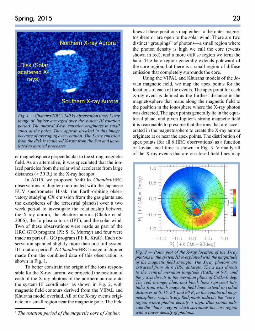
The HRC continues to operate smoothly after more than 15 yrs in orbit, with no significant anoma-lies. The HRC has been used for a wide range of sci-entific investigations over the past year. In this year’s edition of the newsletter, we present results from an HRC observation of Jupiter taken in April 2014 as part of a large international campaign to study the Jovian aurora, inner magnetosphere, and Io plasma torus.

Early Chandra observations of Jupiter showed that the X-ray flux was dominated by two hot spots at the magnetic poles at latitudes poleward of the mag-netic flux lines that map to Io (Gladstone et al. 2002, Elsner et al. 2003, Elsner et al. 2005). The primary X-ray emission process is charge exchange (CX) be-tween neutrals in the Jovian atmosphere and energetic ions accelerated in an electric field parallel to the mag-netic field (Cravens et al. 2003, Bunce et al. 2004). The origin of the ions responsible for the X-ray auro-ra is still an open question, and determining whether they originate from Io or the solar wind has important implications for our understanding about matter and energy transport in the magnetosphere, and the inter-action between the magnetosphere and the solar wind. In the magnetic-dominated plasma of the inner mag-netosphere, it is difficult to understand how ionized particles originating on Io could propagate to the out-

23Spring, 2015

er magnetosphere perpendicular to the strong magnetic field. As an alternative, it was speculated that the ion-ized particles from the solar wind accelerate from large distances (> 30 RJ) to the X-ray hot spot.

In AO15, we proposed 6×40 ks Chandra/HRC observations of Jupiter coordinated with the Japanese EUV spectrometer Hisaki (an Earth-orbiting obser-vatory studying CX emission from the gas giants and the exospheres of the terrestrial planets) over a two week period to investigate the relationship between the X-ray aurora, the electron aurora (Clarke et al. 2006), the Io plasma torus (IPT), and the solar wind. Two of these observations were made as part of the HRC GTO program (PI: S. S. Murray) and four were made as part of a GO program (PI: R. Kraft). Each ob-servation spanned slightly more than one full system III rotation period1. A Chandra/HRC image of Jupiter made from the combined data of this observation is shown in Fig. 1.

To better constrain the origin of the ions respon-sible for the X-ray aurora, we projected the position of each of the X-ray photons of the northern aurora onto the system III coordinates, as shown in Fig. 2, with magnetic field contours derived from the VIPAL and Khurana model overlaid. All of the X-ray events origi-nate in a small region near the magnetic pole. The field

1 The rotation period of the magnetic core of Jupiter.

Fig. 1 — Chandra/HRC (240 ks observation time) X-ray image of Jupiter averaged over the system III rotation period. The auroral X-ray emission originates in small spots at the poles. They appear streaked in this image because of averaging over rotation. The X-ray emission from the disk is scattered X-rays from the Sun and unre-lated to auroral processes.

lines at these positions map either to the outer magne-tosphere or are open to the solar wind. There are two distinct “groupings” of photons—a small region where the photon density is high we call the core (events shown in red), and a more diffuse region we term the halo. The halo region generally extends poleward of the core region, but there is a small region of diffuse emission that completely surrounds the core.

Using the VIPAL and Khurana models of the Jo-vian magnetic field, we map the apex points for the locations of each of the events. The apex point for each X-ray event is defined as the furthest distance in the magnetosphere that maps along the magnetic field to the position in the ionosphere where the X-ray photon was detected. The apex points generally lie in the equa-torial plane, and given Jupiter’s strong magnetic field it is reasonable to presume that the ions that are accel-erated in the magnetosphere to create the X-ray aurora originate at or near the apex points. The distribution of apex points (for all 6 HRC observations) as a function of Jovian local time is shown in Fig. 3. Virtually all of the X-ray events that are on closed field lines map

Fig. 2 — Polar plot of the X-ray location of the X-ray photons in the system III overplotted with the magnitude of the magnetic field strength. The X-ray photons are extracted from all 6 HRC datasets. The x axis directs to the central meridian longitude (CML) of 90°, and the y axis directs to the meridian plane of CML=0 deg. The red, orange, blue, and black lines represent lati-tudes from which magnetic field lines extend to radial distances at 6, 15, 30, and 80 RJ in the equatorial mag-netosphere, respectively. Red points indicate the “core” region where photon density is high. Blue points indi-cate the “halo” region which surrounds the core region with a lower density of photons.

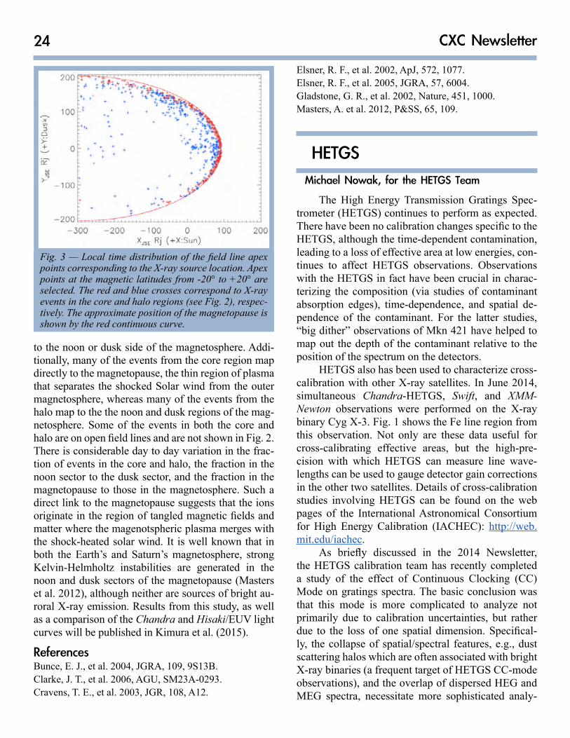
24 CXC Newsletter

to the noon or dusk side of the magnetosphere. Addi-tionally, many of the events from the core region map directly to the magnetopause, the thin region of plasma that separates the shocked Solar wind from the outer magnetosphere, whereas many of the events from the halo map to the the noon and dusk regions of the mag-netosphere. Some of the events in both the core and halo are on open field lines and are not shown in Fig. 2. There is considerable day to day variation in the frac-tion of events in the core and halo, the fraction in the noon sector to the dusk sector, and the fraction in the magnetopause to those in the magnetosphere. Such a direct link to the magnetopause suggests that the ions originate in the region of tangled magnetic fields and matter where the magenotspheric plasma merges with the shock-heated solar wind. It is well known that in both the Earth’s and Saturn’s magnetosphere, strong Kelvin-Helmholtz instabilities are generated in the noon and dusk sectors of the magnetopause (Masters et al. 2012), although neither are sources of bright au-roral X-ray emission. Results from this study, as well as a comparison of the Chandra and Hisaki/EUV light curves will be published in Kimura et al. (2015).

ReferencesBunce, E. J., et al. 2004, JGRA, 109, 9S13B. Clarke, J. T., et al. 2006, AGU, SM23A-0293. Cravens, T. E., et al. 2003, JGR, 108, A12.

Fig. 3 — Local time distribution of the field line apex points corresponding to the X-ray source location. Apex points at the magnetic latitudes from -20° to +20° are selected. The red and blue crosses correspond to X-ray events in the core and halo regions (see Fig. 2), respec-tively. The approximate position of the magnetopause is shown by the red continuous curve.

Elsner, R. F., et al. 2002, ApJ, 572, 1077. Elsner, R. F., et al. 2005, JGRA, 57, 6004. Gladstone, G. R., et al. 2002, Nature, 451, 1000. Masters, A. et al. 2012, P&SS, 65, 109.

HETGSMichael Nowak, for the HETGS Team

The High Energy Transmission Gratings Spec-trometer (HETGS) continues to perform as expected. There have been no calibration changes specific to the HETGS, although the time-dependent contamination, leading to a loss of effective area at low energies, con-tinues to affect HETGS observations. Observations with the HETGS in fact have been crucial in charac-terizing the composition (via studies of contaminant absorption edges), time-dependence, and spatial de-pendence of the contaminant. For the latter studies, “big dither” observations of Mkn 421 have helped to map out the depth of the contaminant relative to the position of the spectrum on the detectors.

HETGS also has been used to characterize cross- calibration with other X-ray satellites. In June 2014, simultaneous Chandra-HETGS, Swift, and XMM- Newton observations were performed on the X-ray binary Cyg X-3. Fig. 1 shows the Fe line region from this observation. Not only are these data useful for cross-calibrating effective areas, but the high-pre-cision with which HETGS can measure line wave-lengths can be used to gauge detector gain corrections in the other two satellites. Details of cross-calibration studies involving HETGS can be found on the web pages of the International Astronomical Consortium for High Energy Calibration (IACHEC): http://web.mit.edu/iachec.

As briefly discussed in the 2014 Newsletter, the HETGS calibration team has recently completed a study of the effect of Continuous Clocking (CC) Mode on gratings spectra. The basic conclusion was that this mode is more complicated to analyze not primarily due to calibration uncertainties, but rather due to the loss of one spatial dimension. Specifical-ly, the collapse of spatial/spectral features, e.g., dust scattering halos which are often associated with bright X-ray binaries (a frequent target of HETGS CC-mode observations), and the overlap of dispersed HEG and MEG spectra, necessitate more sophisticated analy-

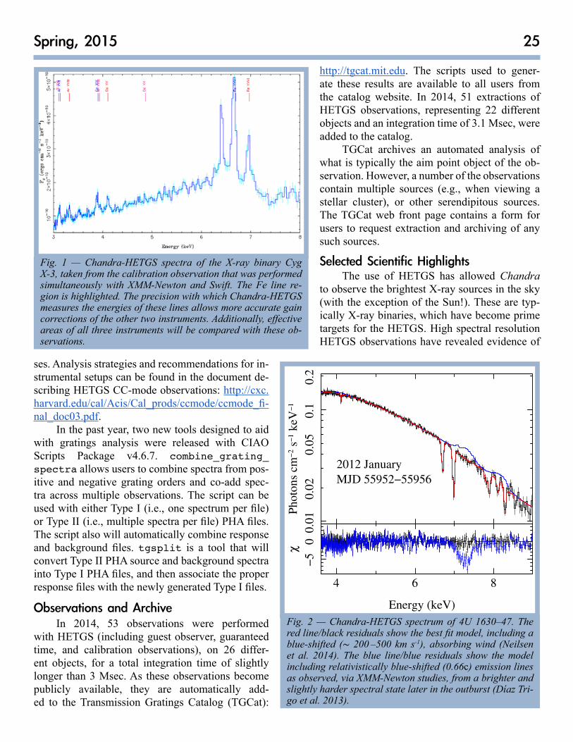
25Spring, 2015

Fig. 1 — Chandra-HETGS spectra of the X-ray binary Cyg X-3, taken from the calibration observation that was performed simultaneously with XMM-Newton and Swift. The Fe line re-gion is highlighted. The precision with which Chandra-HETGS measures the energies of these lines allows more accurate gain corrections of the other two instruments. Additionally, effective areas of all three instruments will be compared with these ob-servations.

ses. Analysis strategies and recommendations for in-strumental setups can be found in the document de-scribing HETGS CC-mode observations: http://cxc.harvard.edu/cal/Acis/Cal_prods/ccmode/ccmode_fi-nal_doc03.pdf.

In the past year, two new tools designed to aid with gratings analysis were released with CIAO Scripts Package v4.6.7. combine_grating_spectra allows users to combine spectra from pos-itive and negative grating orders and co-add spec-tra across multiple observations. The script can be used with either Type I (i.e., one spectrum per file) or Type II (i.e., multiple spectra per file) PHA files. The script also will automatically combine response and background files. tgsplit is a tool that will convert Type II PHA source and background spectra into Type I PHA files, and then associate the proper response files with the newly generated Type I files.

Observations and ArchiveIn 2014, 53 observations were performed

with HETGS (including guest observer, guaranteed time, and calibration observations), on 26 differ-ent objects, for a total integration time of slightly longer than 3 Msec. As these observations become publicly available, they are automatically add-ed to the Transmission Gratings Catalog (TGCat):

http://tgcat.mit.edu. The scripts used to gener-ate these results are available to all users from the catalog website. In 2014, 51 extractions of HETGS observations, representing 22 different objects and an integration time of 3.1 Msec, were added to the catalog.

TGCat archives an automated analysis of what is typically the aim point object of the ob-servation. However, a number of the observations contain multiple sources (e.g., when viewing a stellar cluster), or other serendipitous sources. The TGCat web front page contains a form for users to request extraction and archiving of any such sources.

Selected Scientific HighlightsThe use of HETGS has allowed Chandra

to observe the brightest X-ray sources in the sky (with the exception of the Sun!). These are typ-ically X-ray binaries, which have become prime targets for the HETGS. High spectral resolution HETGS observations have revealed evidence of

Fig. 2 — Chandra-HETGS spectrum of 4U 1630–47. The red line/black residuals show the best fit model, including a blue-shifted (∼ 200 –500 km s-1), absorbing wind (Neilsen et al. 2014). The blue line/blue residuals show the model including relativistically blue-shifted (0.66c) emission lines as observed, via XMM-Newton studies, from a brighter and slightly harder spectral state later in the outburst (Díaz Tri-go et al. 2013).

0.0

10.1

0.0

20.0

50.2

Photo

ns

cm−

2 s

−1 k

eV−

1

2012 January

MJD 55952−55956

4 6 8

−5

0

χ

Energy (keV)

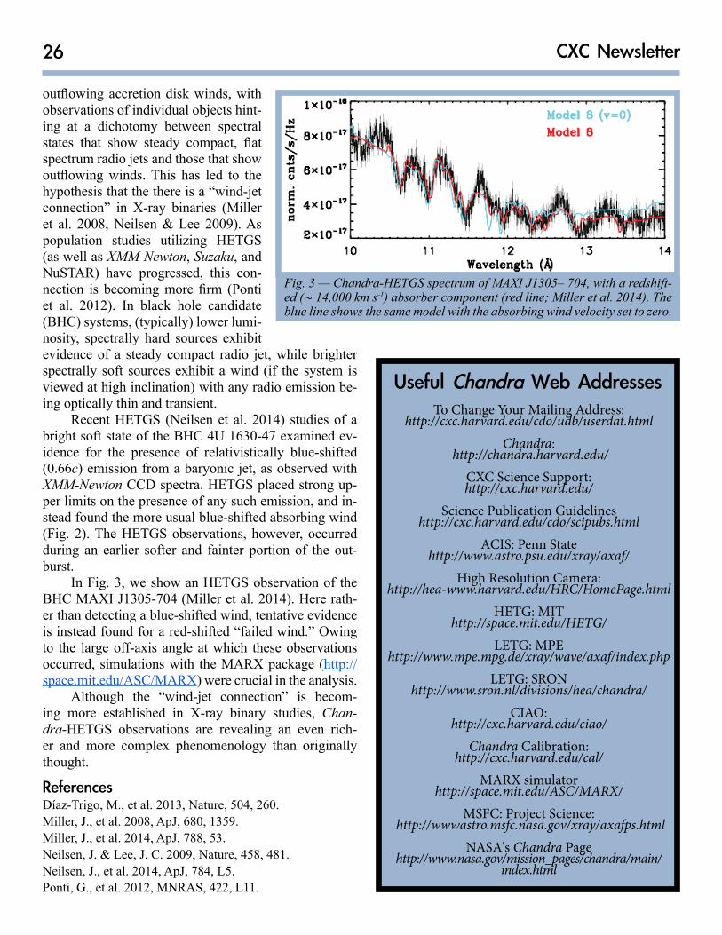
26 CXC Newsletter

Useful Chandra Web AddressesTo Change Your Mailing Address:

http://cxc.harvard.edu/cdo/udb/userdat.htmlChandra:

http://chandra.harvard.edu/ CXC Science Support:http://cxc.harvard.edu/

Science Publication Guidelineshttp://cxc.harvard.edu/cdo/scipubs.html

ACIS: Penn Statehttp://www.astro.psu.edu/xray/axaf/

High Resolution Camera:http://hea-www.harvard.edu/HRC/HomePage.html

HETG: MIThttp://space.mit.edu/HETG/

LETG: MPEhttp://www.mpe.mpg.de/xray/wave/axaf/index.php

LETG: SRONhttp://www.sron.nl/divisions/hea/chandra/

CIAO:http://cxc.harvard.edu/ciao/

Chandra Calibration:http://cxc.harvard.edu/cal/

MARX simulatorhttp://space.mit.edu/ASC/MARX/

MSFC: Project Science: http://wwwastro.msfc.nasa.gov/xray/axafps.html

NASA's Chandra Pagehttp://www.nasa.gov/mission_pages/chandra/main/

index.html

outflowing accretion disk winds, with observations of individual objects hint-ing at a dichotomy between spectral states that show steady compact, flat spectrum radio jets and those that show outflowing winds. This has led to the hypothesis that the there is a “wind-jet connection” in X-ray binaries (Miller et al. 2008, Neilsen & Lee 2009). As population studies utilizing HETGS (as well as XMM-Newton, Suzaku, and NuSTAR) have progressed, this con-nection is becoming more firm (Ponti et al. 2012). In black hole candidate (BHC) systems, (typically) lower lumi-nosity, spectrally hard sources exhibit evidence of a steady compact radio jet, while brighter spectrally soft sources exhibit a wind (if the system is viewed at high inclination) with any radio emission be-ing optically thin and transient.

Recent HETGS (Neilsen et al. 2014) studies of a bright soft state of the BHC 4U 1630-47 examined ev-idence for the presence of relativistically blue-shifted (0.66c) emission from a baryonic jet, as observed with XMM-Newton CCD spectra. HETGS placed strong up-per limits on the presence of any such emission, and in-stead found the more usual blue-shifted absorbing wind (Fig. 2). The HETGS observations, however, occurred during an earlier softer and fainter portion of the out-burst.

In Fig. 3, we show an HETGS observation of the BHC MAXI J1305-704 (Miller et al. 2014). Here rath-er than detecting a blue-shifted wind, tentative evidence is instead found for a red-shifted “failed wind.” Owing to the large off-axis angle at which these observations occurred, simulations with the MARX package (http://space.mit.edu/ASC/MARX) were crucial in the analysis.

Although the “wind-jet connection” is becom-ing more established in X-ray binary studies, Chan-dra-HETGS observations are revealing an even rich-er and more complex phenomenology than originally thought.

ReferencesDíaz-Trigo, M., et al. 2013, Nature, 504, 260.Miller, J., et al. 2008, ApJ, 680, 1359.Miller, J., et al. 2014, ApJ, 788, 53.Neilsen, J. & Lee, J. C. 2009, Nature, 458, 481.Neilsen, J., et al. 2014, ApJ, 784, L5.Ponti, G., et al. 2012, MNRAS, 422, L11.

Fig. 3 — Chandra-HETGS spectrum of MAXI J1305– 704, with a redshift-ed (∼ 14,000 km s-1) absorber component (red line; Miller et al. 2014). The blue line shows the same model with the absorbing wind velocity set to zero.

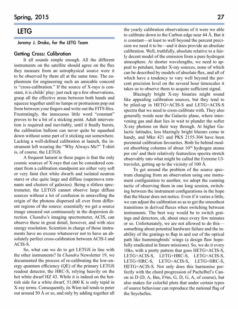
27Spring, 2015

LETGJeremy J. Drake, for the LETG Team

Getting Cross: CalibrationIt all sounds simple enough. All the different

instruments on the satellite should agree on the flux they measure from an astrophysical source were it to be observed by them all at the same time. The eu-phemism for engineering such an amicable concord is “cross-calibration.” If the source of X-rays is con-stant, it is childs’ play: just rack up a few observations, grasp all the effective areas between both hands and squeeze together until no lumps or protrusions pop out from between your fingers and write out the FITS files. Frustratingly, the innocuous little word “constant” proves to be a bit of a sticking point. Adult interven-tion is required and inevitably, until it finally bursts, the calibration balloon can never quite be squashed down without some part of it sticking out somewhere. Lacking a well-defined calibration at launch, the in-strument left wearing the “Why Always Me?” T-shirt is, of course, the LETGS.

A frequent lament in these pages is that the only cosmic sources of X-rays that can be considered con-stant from a calibration standpoint are either very soft or very faint (hot white dwarfs and isolated neutron stars) or else quite large and diffuse (supernova rem-nants and clusters of galaxies). Being a slitless spec-trometer, the LETGS cannot observe large diffuse sources without a lot of confusion in unravelling the origin of the photons dispersed all over from differ-ent regions of the source: essentially we get a source image smeared out continuously in the dispersion di-rection. Chandra’s imaging spectrometer, ACIS, can observe these in great detail, however, and with nice energy resolution. Scientists in charge of those instru-ments have no excuse whatsoever not to have an ab-solutely perfect cross-calibration between ACIS-I and ACIS-S.

So, what can we do to get LETGS in line with the other instruments? In Chandra Newsletter 19, we documented the process of re-calibrating the low-en-ergy quantum efficiency (QE) of the primary LETGS readout detector, the HRC-S, relying heavily on the hot white dwarf HZ 43. While it is indeed on the hot-tish side for a white dwarf, 51,000 K is only tepid in X-ray terms. Consequently, its Wien tail tends to peter out around 50 Å or so, and only by adding together all

the yearly calibration observations of it were we able to calibrate down to the Carbon edge near 44 Å. But it is constant—at least to well beyond the percent preci-sion we need it to be—and it does provide an absolute calibration. Well, truthfully, absolute relative to a fair-ly decent model of the emission from a pure hydrogen atmosphere. At shorter wavelengths, we need to ap-peal to petulant, harder X-ray sources, none of which can be described by models of absolute flux, and all of which have a tendency to vary well beyond the per-cent precision level on the several hour timescales it takes us to observe them to acquire sufficient signal.

Blazingly bright X-ray binaries might sound like appealing calibration sources, but they tend to be piled-up in HETG+ACIS-S and LETG+ACIS-S spectra that we need to cross-calibrate with. They also generally reside near the Galactic plane, where inter-vening gas and dust lies in wait to plunder the softer X-ray photons on their way through. At higher Ga-lactic latitudes, less blazingly bright blazars come in handy, and Mkn 421 and PKS 2155-304 have been perennial calibration favourites. Both lie behind mod-est absorbing columns of about 1020 hydrogen atoms per cm2 and their relatively featureless spectra stretch observably into what might be called the Extreme Ul-traviolet, getting up to the vicinity of 100 Å.

To get around the problem of the source spec-trum changing from an observation using one instru-ment configuration to another, we adopt the cunning tactic of observing them in one long session, switch-ing between the instrument configurations in the hope that the blazar does not notice. Even if it varies a little, we can adjust the calibration so as to get the smoothest transitions in derived fluxes when switching between instruments. The best way would be to switch grat-ings and detectors, oh, about once every few minutes or so. Unfortunately, we are not allowed to do this—something about potential hardware failure and the in-ability of the gratings to flap in and out of the optical path like hummingbirds’ wings (a design flaw hope-fully eradicated in future missions). So, we do it every 10ks, with a pretty pattern that goes HETG+ACIS-S, LETG+ACIS-S, LETG+HRC-S, LETG+ACIS-S, LETG+HRC-S, LETG+ACIS-S, LETG+HRC-S, HETG+ACIS-S. Not only does this harmonise per-fectly with the chord progression of Pachelbel’s Can-on in D (D, A, Bm, F#m, G, D, G, A, of course), but also makes for colorful plots that under certain types of source behaviour can reproduce the national flag of the Seychelles.

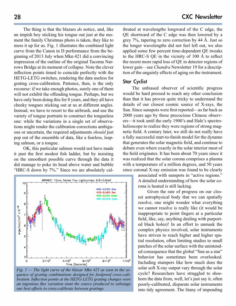
28 CXC Newsletter

The thing is that the blazars do notice, and, like an impish boy sticking his tongue out just at the mo-ment the family Christmas photo is taken, they like to mess it up for us. Fig. 1 illustrates the combined light curve from the Canon in D performance from the be-ginning of 2013 July when Mkn 421 did a convincing impression of the outline of the original Tacoma Nar-rows Bridge at its moment of collapse. Note the clever inflection points timed to coincide perfectly with the HETG-LETG switches, rendering the data useless for grating cross-calibration. Patience, then, is the only recourse: if we take enough photos, surely one of them will not exhibit the offending tongue. Perhaps, but we have only been doing this for 8 years, and they all have cheeky tongues sticking out at us at different angles. Instead, we have to resort to the airbrush, and use the variety of tongue portraits to construct the tongueless one: while the variations in a single set of observa-tions might render the calibration corrections ambigu-ous or uncertain, the required adjustments should just pop out of the ensemble of data, like a fearless, leap-ing salmon, or a tongue.

OK, this particular salmon would not have made it past the first modest fish ladder, but by insisting on the smoothest possible curve through the data it did manage to poke its head above water and bubble “HRC-S down by 7%.” Since we are absolutely cal-

Fig. 1 — The light curve of the blazar Mkn 421 as seen in the se-quence of grating combinations designed for foolproof cross-cali-bration. Inflection points at the HETG-LETG grating changes were an ingenious flux variation stunt the source produced to sabotage our best efforts to cross-calibrate between gratings.

ibrated at wavelengths longward of the C edge, the QE shortward of the C edge was then lowered by a grey 7%, tapering to zero correction by 44 Å. Just so the longer wavelengths did not feel left out, we also applied some few percent time-dependent QE tweaks to the HRC-S QE in the vicinity of 100 Å to reflect the recent more rapid loss of QE in detector regions of lower gain—see Chandra Newsletter 19 for a descrip-tion of the ungainly effects of aging on the instrument.

Star CyclistThe unbiased observer of scientific progress

would be hard pressed to reach any other conclusion than that it has proven quite tricky to understand the details of our closest cosmic source of X-rays, the Sun. Since sunspots were first reported—as far back as 2000 years ago by those precocious Chinese observ-ers—it took until the early 1900’s and Hale’s spectro-helioscope to realize they were regions of strong mag-netic field. A century later, we still do not really have a fully successful start-to-finish model for the dynamo that generates the solar magnetic field, and continue to debate even where exactly in the solar interior most of the field originates. It has been about 70 years since it was realized that the solar corona comprises a plasma with a temperature of a million degrees, and 50 years since coronal X-ray emission was found to be clearly

associated with sunspots in “active regions.” A detailed understanding of how the solar co-rona is heated is still lacking.

Given the rate of progress on our clos-est astrophysical body that we can spatially resolve, one might wonder what everything we cannot resolve is really like (it would be inappropriate to point fingers at a particular field, like, say, anything dealing with purport-ed black holes)! In an effort to unmask the complex physics involved, solar instruments have striven to reach higher and higher spa-tial resolution, often limiting studies to small patches of the solar surface with the unintend-ed consequence that the global “Sun as a star” behavior has sometimes been overlooked. Including stumpers like how much does the solar soft X-ray output vary through the solar cycle? Researchers have struggled to shoe-horn the data from, well, let’s just say it, often poorly-calibrated, disparate solar instruments into tidy agreement. The litany of impending

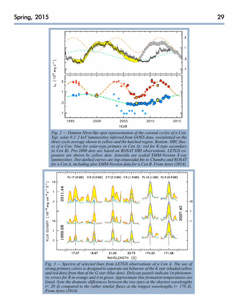
29Spring, 2015

Fig. 2 — Damien Hirst-like spot representation of the coronal cycles of α Cen. Top: solar 0.2–2 keV luminosities inferred from GOES data, overplotted on the three-cycle average shown in yellow and the hatched region. Bottom: HRC flux-es of α Cen: blue for solar-type primary (α Cen A); red for K-type secondary (α Cen B). Pre-2000 dots are based on ROSAT HRI observations. LETGS ex-posures are shown by yellow dots. Asterisks are scaled XMM-Newton X-ray luminosities. Dot-dashed curves are log-sinusoidal fits to Chandra and ROSAT for α Cen A, including also XMM-Newton data for α Cen B. From Ayres (2014).

Fig. 3 — Spectra of selected lines from LETGS observations of α Cen A. The use of strong primary colors is designed to separate out behavior of the K star (shaded yellow and red dots) from that of the G star (blue dots). Delicate pastels indicate 1σ photomet-ric errors for B in orange and A in green. Approximate line formation temperatures are listed. Note the dramatic differences between the two stars at the shortest wavelengths (< 20 Å) compared to the rather similar fluxes at the longest wavelengths (> 170 Å). From Ayres (2014).

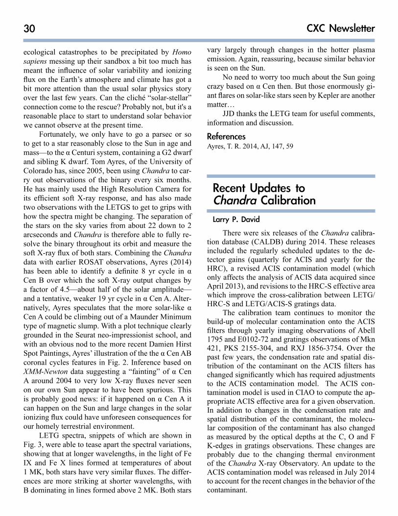
30 CXC Newsletter

ecological catastrophes to be precipitated by Homo sapiens messing up their sandbox a bit too much has meant the influence of solar variability and ionizing flux on the Earth’s atmosphere and climate has got a bit more attention than the usual solar physics story over the last few years. Can the cliché “solar-stellar” connection come to the rescue? Probably not, but it's a reasonable place to start to understand solar behavior we cannot observe at the present time.

Fortunately, we only have to go a parsec or so to get to a star reasonably close to the Sun in age and mass—to the α Centuri system, containing a G2 dwarf and sibling K dwarf. Tom Ayres, of the University of Colorado has, since 2005, been using Chandra to car-ry out observations of the binary every six months. He has mainly used the High Resolution Camera for its efficient soft X-ray response, and has also made two observations with the LETGS to get to grips with how the spectra might be changing. The separation of the stars on the sky varies from about 22 down to 2 arcseconds and Chandra is therefore able to fully re-solve the binary throughout its orbit and measure the soft X-ray flux of both stars. Combining the Chandra data with earlier ROSAT observations, Ayres (2014) has been able to identify a definite 8 yr cycle in α Cen B over which the soft X-ray output changes by a factor of 4.5—about half of the solar amplitude—and a tentative, weaker 19 yr cycle in α Cen A. Alter-natively, Ayres speculates that the more solar-like α Cen A could be climbing out of a Maunder Minimum type of magnetic slump. With a plot technique clearly grounded in the Seurat neo-impressionist school, and with an obvious nod to the more recent Damien Hirst Spot Paintings, Ayres’ illustration of the the α Cen AB coronal cycles features in Fig. 2. Inference based on XMM-Newton data suggesting a “fainting” of α Cen A around 2004 to very low X-ray fluxes never seen on our own Sun appear to have been spurious. This is probably good news: if it happened on α Cen A it can happen on the Sun and large changes in the solar ionizing flux could have unforeseen consequences for our homely terrestrial environment.

LETG spectra, snippets of which are shown in Fig. 3, were able to tease apart the spectral variations, showing that at longer wavelengths, in the light of Fe IX and Fe X lines formed at temperatures of about 1 MK, both stars have very similar fluxes. The differ-ences are more striking at shorter wavelengths, with B dominating in lines formed above 2 MK. Both stars

vary largely through changes in the hotter plasma emission. Again, reassuring, because similar behavior is seen on the Sun.

No need to worry too much about the Sun going crazy based on α Cen then. But those enormously gi-ant flares on solar-like stars seen by Kepler are another matter…

JJD thanks the LETG team for useful comments, information and discussion.

ReferencesAyres, T. R. 2014, AJ, 147, 59

Recent Updates to Chandra CalibrationLarry P. David

There were six releases of the Chandra calibra-tion database (CALDB) during 2014. These releases included the regularly scheduled updates to the de-tector gains (quarterly for ACIS and yearly for the HRC), a revised ACIS contamination model (which only affects the analysis of ACIS data acquired since April 2013), and revisions to the HRC-S effective area which improve the cross-calibration between LETG/HRC-S and LETG/ACIS-S gratings data.

The calibration team continues to monitor the build-up of molecular contamination onto the ACIS filters through yearly imaging observations of Abell 1795 and E0102-72 and gratings observations of Mkn 421, PKS 2155-304, and RXJ 1856-3754. Over the past few years, the condensation rate and spatial dis-tribution of the contaminant on the ACIS filters has changed significantly which has required adjustments to the ACIS contamination model. The ACIS con-tamination model is used in CIAO to compute the ap-propriate ACIS effective area for a given observation. In addition to changes in the condensation rate and spatial distribution of the contaminant, the molecu-lar composition of the contaminant has also changed as measured by the optical depths at the C, O and F K-edges in gratings observations. These changes are probably due to the changing thermal environment of the Chandra X-ray Observatory. An update to the ACIS contamination model was released in July 2014 to account for the recent changes in the behavior of the contaminant.

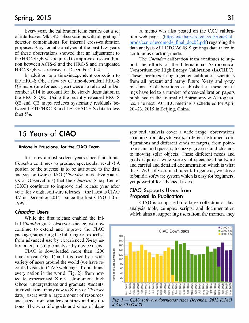
31Spring, 2015

Every year, the calibration team carries out a set of interleaved Mkn 421 observations with all gratings/detector combinations for internal cross-calibration purposes. A systematic analysis of the past few years of these observations showed that an adjustment to the HRC-S QE was required to improve cross-calibra-tion between ACIS-S and the HRC-S and an updated HRC-S QE was released in December 2014.

In addition to a time-independent correction to the HRC-S QE, a new set of time-dependent HRC-S QE maps (one for each year) was also released in De-cember 2014 to account for the steady degradation in the HRC-S QE. Using the recently released HRC-S QE and QE maps reduces systematic residuals be-tween LETG/HRC-S and LETG/ACIS-S data to less than 5%.

A memo was also posted on the CXC calibra-tion web pages (http://cxc.harvard.edu/cal/Acis/Cal_prods/ccmode/ccmode_final_doc02.pdf) regarding the data analysis of HETG/ACIS-S gratings data taken in continuous clocking mode.

The Chandra calibration team continues to sup-port the efforts of the International Astronomical Consortium for High Energy Calibration (IACHEC). These meetings bring together calibration scientists from all present and many future X-ray and γ-ray missions. Collaborations established at these meet-ings have led to a number of cross-calibration papers published in the Journal of Astronomy & Astrophys-ics. The next IACHEC meeting is scheduled for April 20 –23, 2015 in Beijing, China.

15 Years of CIAO

Antonella Fruscione, for the CIAO Team

It is now almost sixteen years since launch and Chandra continues to produce spectacular results! A portion of the success is to be attributed to the data analysis software CIAO (Chandra Interactive Analy-sis of Observations) that the Chandra X-ray Center (CXC) continues to improve and release year after year: forty eight software releases—the latest is CIAO 4.7 in December 2014—since the first CIAO 1.0 in 1999.

Chandra UsersWhile the first release enabled the ini-

tial Chandra guest observer science, we now continue to extend and improve the CIAO package, supporting the full range of expertise from advanced use by experienced X-ray as-tronomers to simple analysis by novice users.

CIAO is downloaded more than 1200 times a year (Fig. 1) and it is used by a wide variety of users around the world (we have re-corded visits to CIAO web pages from almost every nation in the world, Fig. 2): from nov-ice to experienced X-ray astronomers, high school, undergraduate and graduate students, archival users (many new to X-ray or Chandra data), users with a large amount of resources, and users from smaller countries and institu-tions. The scientific goals and kinds of data-

Fig. 1 — CIAO software downloads since December 2012 (CIAO 4.5 to CIAO 4.7).

sets and analysis cover a wide range: observations spanning from days to years, different instrument con-figurations and different kinds of targets, from point-like stars and quasars, to fuzzy galaxies and clusters, to moving solar objects. These different needs and goals require a wide variety of specialized software and careful and detailed documentation which is what the CIAO software is all about. In general, we strive to build a software system which is easy for beginners, yet powerful for advanced users.

CIAO Supports Users from Proposal to Publication

CIAO is comprised of a large collection of data analysis tools, complex scripts, and documentation which aims at supporting users from the moment they

32 CXC Newsletter

plan a Chandra observation to when they are ready to publish a paper (Fig. 3). In addition, except for a few instrument-specific tools, most tools can be used for the analysis of other X-ray and even non X-ray data.

At the proposal planning stage CIAO can be used to assess the feasibility of an observation and to ex-amine the Chandra field-of-view (e.g., with tools like colden and obsvis), it can be used for batch archive and catalog searches (e.g., find_chandra_obsid, download_chandra_obsid, search_csc) and to inspect and explore data sets (What is this dataset? How many photons? What is the instrument configura-tion? Quick look visualization, e.g., with ds9, prism, dmlist, dmstat, dmcopy). When it is time for de-

Fig. 2 — Access to CIAO webpages from all over the world over an approximately two year period.

tailed data reduction, tools are available to apply the latest calibrations to an observation, to locate sources and measure their properties (position, brightness, and variability), and for each source, to generate tailored calibration files (e.g., spectral calibration) via tools like dmextract, wavdetect, specextract, srcflux, and fluximage.

In the final stages of the analysis, the Sherpa application (the CIAO 1D and 2D modeling and fitting package) is invoked. Sherpa is built via a Python interface, which is familiar to the new generation of astronomers and widely used by other missions. Finally, the ChIPS application can be invoked to prepare publication quality graphics.

Documentation and Community SupportOne of the most praised characteristics of CIAO

is the extent of the documentation that accompanies the data analysis system. CIAO documentation spans over 2000 web pages including FAQ, plot galleries, dictionaries, caveats, tips and tricks, bug notes, etc. There are about 200 science-task-oriented, step-by-step, end-to-end, analysis “threads” and about 1000 help files for individual tools and concepts. The latest addition to our outreach effort are YouTube tutorials to walk users through the more interactive tasks.

Personal and prompt support to CIAO users is another aspect of which we are proud. The CXC Help-desk receives hundreds of CIAO-related queries every

Fig. 3 — Flowchart with the CIAO tools that help users from proposal planning to publication.

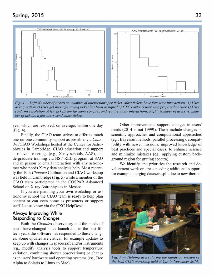
33Spring, 2015

Fig. 4 — Left: Number of tickets vs. number of interactions per ticket. Most tickets have four user interactions: 1) User asks question 2) User get message saying ticket has been assigned 3) CXC contacts user with proposed answer 4) User confirms resolution. A few tickets are far more complex and require many interactions. Right: Number of users vs. num-ber of tickets: a few users send many tickets.

year which are resolved, on average, within one day (Fig. 4).

Finally, the CIAO team strives to offer as much one-on-one community support as possible, via Chan-dra/CIAO Workshops hosted at the Center for Astro-physics in Cambridge, CIAO education and support at relevant meetings (e.g., X-ray schools, AAS), un-dergraduate training via NSF REU program at SAO and in person or email interaction with any astrono-mer who needs X-ray data analysis help. Most recent-ly the 10th Chandra Calibration and CIAO workshop was held in Cambridge (Fig. 5) while a member of the CIAO team participated in the COSPAR Advanced School on X-ray Astrophysics in Mexico.

If you are planning your own workshop or as-tronomy school the CIAO team is ready to help plan content or can even come as presenters or support staff. Let us know via the CXC HelpDesk.

Always Improving While Responding to Changes

Both the Chandra observatory and the needs of users have changed since launch and in the past fif-teen years the software has responded to these chang-es. Some updates are critical, for example updates to keep up with changes in spacecraft and/or instruments (eg., modify analysis tools to support temperature variation, combining shorter observations) or chang-es in users' hardware and operating systems (eg., Dec Alpha to Solaris to Linux to Mac).

Other improvements support changes in users' needs (2014 is not 1999!). These include changes in scientific approaches and computational approaches (eg., Bayesian methods, parallel processing); compat-ibility with newer missions; improved knowledge of best practices and special cases, to enhance science and minimize mistakes (eg., applying custom back-ground region for grating spectra).

We identify and prioritize the research and de-velopment work on areas needing additional support, for example merging datasets split due to new thermal

Fig. 5 — Helping users during the hands-on session of the 10th CIAO workshop held at CfA in November 2014.

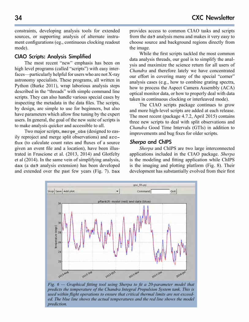
34 CXC Newsletter

constraints, developing analysis tools for extended sources, or supporting analysis of alternate instru-ment configurations (eg., continuous clocking readout mode).

CIAO Scripts: Analysis SimplifiedThe most recent “new” emphasis has been on

high level programs (called “scripts”) with easy inter-faces—particularly helpful for users who are not X-ray astronomy specialists. These programs, all written in Python (Burke 2011), wrap laborious analysis steps described in the “threads” with simple command line scripts. They can also handle various special cases by inspecting the metadata in the data files. The scripts, by design, are simple to use for beginners, but also have parameters which allow fine tuning by the expert users. In general, the goal of the new suite of scripts is to make analysis quicker and accessible to all.

Two major scripts, merge_obs (designed to eas-ily reproject and merge split observations) and src-flux (to calculate count rates and fluxes of a source given an event file and a location), have been illus-trated in Fruscione et al. (2013, 2014) and Glotfelty et al (2014). In the same vein of simplifying analysis, dax (a ds9 analysis extension) has been developed and extended over the past few years (Fig. 7). Dax

provides access to common CIAO tasks and scripts from the ds9 analysis menu and makes it very easy to choose source and background regions directly from the image.

While the first scripts tackled the most common data analysis threads, our goal is to simplify the anal-ysis and maximize the science return for all users of Chandra and therefore lately we have concentrated our effort in covering many of the special “corner” analysis cases (e.g., how to combine grating spectra, how to process the Aspect Camera Assembly (ACA) optical monitor data, or how to properly deal with data taken in continuous clocking or interleaved mode).

The CIAO scripts package continues to grow and more high-level scripts are added at each release. The most recent (package 4.7.2, April 2015) contains three new scripts to deal with split observations and Chandra Good Time Intervals (GTIs) in addition to improvements and bug fixes for older scripts.

Sherpa and ChIPSSherpa and ChIPS are two large interconnected

applications included in the CIAO package. Sherpa is the modeling and fitting application while ChIPS is the imaging and plotting platform (Fig. 8). Their development has substantially evolved from their first

Fig. 6 — Graphical fitting tool using Sherpa to fit a 20-parameter model that predicts the temperature of the Chandra Integral Propulsion System tank. This is used within flight operations to ensure that critical thermal limits are not exceed-ed. The blue line shows the actual temperatures and the red line shows the model prediction.

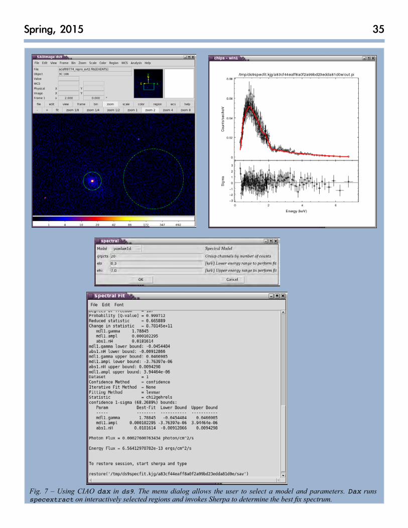
35Spring, 2015

Fig. 7 – Using CIAO dax in ds9. The menu dialog allows the user to select a model and parameters. Dax runs specextract on interactively selected regions and invokes Sherpa to determine the best fix spectrum.

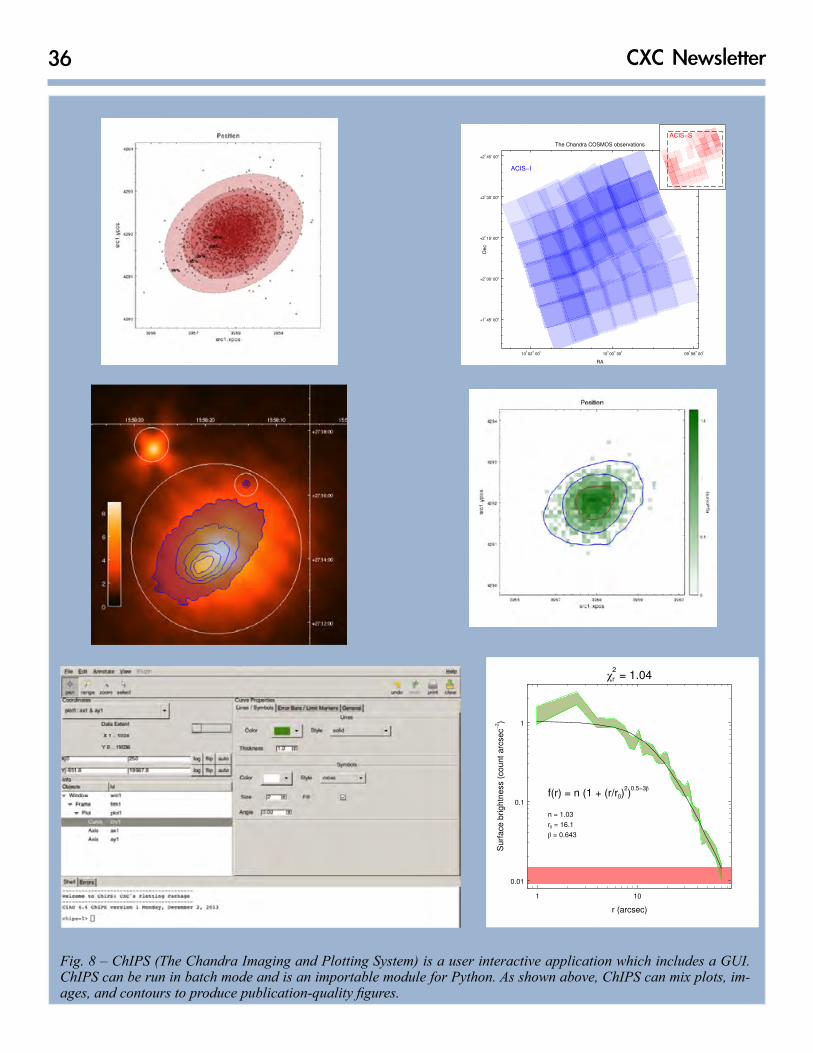
36 CXC Newsletter

c2r = 1.04

r (arcsec)

1 10

Sur

face

brig

htne

ss (

coun

t arc

sec−2

)

0.01

0.1

1

f(r) = n (1 + (r/r0)2)0.5−3b

n = 1.03r0 = 16.1b = 0.643

The Chandra COSMOS observations

RA

10h 02

m 00

s10

h 00

m 00

s09

h 58

m 00

s

Dec

+1o 45’ 00"

+2o 00’ 00"

+2o 15’ 00"

+2o 30’ 00"

+2o 45’ 00"

ACIS−I

ACIS−S

Fig. 8 – ChIPS (The Chandra Imaging and Plotting System) is a user interactive application which includes a GUI. ChIPS can be run in batch mode and is an importable module for Python. As shown above, ChIPS can mix plots, im-ages, and contours to produce publication-quality figures.

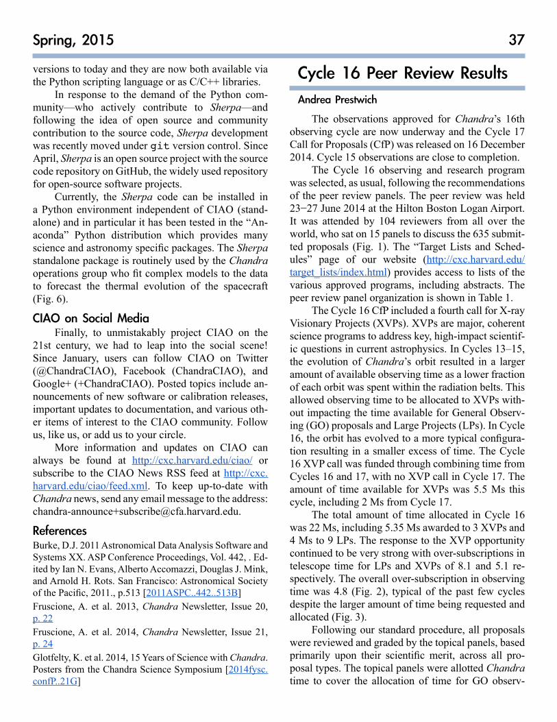
37Spring, 2015

versions to today and they are now both available via the Python scripting language or as C/C++ libraries.

In response to the demand of the Python com-munity—who actively contribute to Sherpa—and following the idea of open source and community contribution to the source code, Sherpa development was recently moved under git version control. Since April, Sherpa is an open source project with the source code repository on GitHub, the widely used repository for open-source software projects.

Currently, the Sherpa code can be installed in a Python environment independent of CIAO (stand-alone) and in particular it has been tested in the “An-aconda” Python distribution which provides many science and astronomy specific packages. The Sherpa standalone package is routinely used by the Chandra operations group who fit complex models to the data to forecast the thermal evolution of the spacecraft (Fig. 6).

CIAO on Social MediaFinally, to unmistakably project CIAO on the

21st century, we had to leap into the social scene! Since January, users can follow CIAO on Twitter (@ChandraCIAO), Facebook (ChandraCIAO), and Google+ (+ChandraCIAO). Posted topics include an-nouncements of new software or calibration releases, important updates to documentation, and various oth-er items of interest to the CIAO community. Follow us, like us, or add us to your circle.

More information and updates on CIAO can always be found at http://cxc.harvard.edu/ciao/ or subscribe to the CIAO News RSS feed at http://cxc.harvard.edu/ciao/feed.xml. To keep up-to-date with Chandra news, send any email message to the address: chandra-announce+subscribe@cfa.harvard.edu.

ReferencesBurke, D.J. 2011 Astronomical Data Analysis Software and Systems XX. ASP Conference Proceedings, Vol. 442, . Ed-ited by Ian N. Evans, Alberto Accomazzi, Douglas J. Mink, and Arnold H. Rots. San Francisco: Astronomical Society of the Pacific, 2011., p.513 [2011ASPC..442..513B]Fruscione, A. et al. 2013, Chandra Newsletter, Issue 20, p. 22Fruscione, A. et al. 2014, Chandra Newsletter, Issue 21, p. 24Glotfelty, K. et al. 2014, 15 Years of Science with Chandra. Posters from the Chandra Science Symposium [2014fysc.confP..21G]

Cycle 16 Peer Review ResultsAndrea Prestwich

The observations approved for Chandra’s 16th observing cycle are now underway and the Cycle 17 Call for Proposals (CfP) was released on 16 December 2014. Cycle 15 observations are close to completion.

The Cycle 16 observing and research program was selected, as usual, following the recommendations of the peer review panels. The peer review was held 23−27 June 2014 at the Hilton Boston Logan Airport. It was attended by 104 reviewers from all over the world, who sat on 15 panels to discuss the 635 submit-ted proposals (Fig. 1). The “Target Lists and Sched-ules” page of our website (http://cxc.harvard.edu/target_lists/index.html) provides access to lists of the various approved programs, including abstracts. The peer review panel organization is shown in Table 1.

The Cycle 16 CfP included a fourth call for X-ray Visionary Projects (XVPs). XVPs are major, coherent science programs to address key, high-impact scientif-ic questions in current astrophysics. In Cycles 13–15, the evolution of Chandra’s orbit resulted in a larger amount of available observing time as a lower fraction of each orbit was spent within the radiation belts. This allowed observing time to be allocated to XVPs with-out impacting the time available for General Observ-ing (GO) proposals and Large Projects (LPs). In Cycle 16, the orbit has evolved to a more typical configura-tion resulting in a smaller excess of time. The Cycle 16 XVP call was funded through combining time from Cycles 16 and 17, with no XVP call in Cycle 17. The amount of time available for XVPs was 5.5 Ms this cycle, including 2 Ms from Cycle 17.

The total amount of time allocated in Cycle 16 was 22 Ms, including 5.35 Ms awarded to 3 XVPs and 4 Ms to 9 LPs. The response to the XVP opportunity continued to be very strong with over-subscriptions in telescope time for LPs and XVPs of 8.1 and 5.1 re-spectively. The overall over-subscription in observing time was 4.8 (Fig. 2), typical of the past few cycles despite the larger amount of time being requested and allocated (Fig. 3).

Following our standard procedure, all proposals were reviewed and graded by the topical panels, based primarily upon their scientific merit, across all pro-posal types. The topical panels were allotted Chandra time to cover the allocation of time for GO observ-

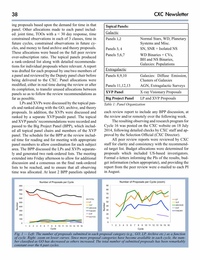
38 CXC Newsletter

Fig. 1 — Left: The number of proposals submitted in each proposal category (e.g., GO, LP, Archive etc.) as a function of cycle. Right: zoom on lower curves. Since more proposal categories have become available in each cycle, the num-ber classified as GO has decreased as others increased. The total number of submitted proposals has been remarkably constant over the 6 past cycles.

Table 1: Panel Organization

ing proposals based upon the demand for time in that panel. Other allocations made to each panel includ-ed: joint time, TOOs with a < 30 day response, time constrained observations in each of 3 classes, time in future cycles, constrained observations in future cy-cles, and money to fund archive and theory proposals. These allocations were based on the full peer review over-subscription ratio. The topical panels produced a rank-ordered list along with detailed recommenda-tions for individual proposals where relevant. A report was drafted for each proposal by one/two members of a panel and reviewed by the Deputy panel chair before being delivered to the CXC. Panel allocations were modified, either in real time during the review or after its completion, to transfer unused allocations between panels so as to follow the review recommendations as far as possible.

LPs and XVPs were discussed by the topical pan-els and ranked along with the GO, archive, and theory proposals. In addition, the XVPs were discussed and ranked by a separate XVP/pundit panel. The topical and XVP panels’ recommendations were recorded and passed to the Big Project Panel (BPP), which includ-ed all topical panel chairs and members of the XVP panel. The schedule for the BPP at the review includ-ed time for reading and for meeting with appropriate panel members to allow coordination for each subject area. The BPP discussed the LPs and XVPs separate-ly and generated two rank-ordered lists. The meeting extended into Friday afternoon to allow for additional discussion and a consensus on the final rank-ordered lists to be reached, and to ensure that all observing time was allocated. At least 2 BPP panelists updated

each review report to include any BPP discussion, at the review and/or remotely over the following week.

The resulting observing and research program for Cycle 16 was posted on the CXC website on 18 July 2014, following detailed checks by CXC staff and ap-proval by the Selection Official (CXC Director).

All peer review reports were reviewed by CXC staff for clarity and consistency with the recommend-ed target list. Budget allocations were determined for proposals which included US-based investigators. Formal e-letters informing the PIs of the results, bud-get information (when appropriate), and providing the report from the peer review were e-mailed to each PI in August.

0

100

200

300

400

500

600

700

800

900

1 2 3 4 5 6 7 8 9 10 11 12 13 14 15 16

Num

ber

Cycle

Number of Proposals per Cycle

TOTAL

LP

VLP

ARCHIVE

THEORY

XVP

GO/TOO

0

10

20

30

40

50

60

70

80

90

1 2 3 4 5 6 7 8 9 10 11 12 13 14 15 16

Num

ber

Cycle

Number of Proposals per Cycle (zoom)

LP VLP ARCHIVE XVP THEORY

Topical Panels:GalacticPanels 1,2 Normal Stars, WD, Planetary

Systems and Misc.Panels 3, 4 SN, SNR + Isolated NSPanels 5,6,7 WD Binaries + CVs,

BH and NS Binaries, Galaxies: Populations

ExtragalacticPanels 8,9,10 Galaxies: Diffuse Emission,

Clusters of GalaxiesPanels 11,12,13 AGN, Extragalactic SurveysXVP Panel X-ray Visionary ProposalsBig Project Panel LP and XVP Proposals

39Spring, 2015

Joint Time AllocationChandra time was also allocated to joint programs

by the proposal review processes of XMM-Newton (1 proposal) and HST (1 proposal).

The Chandra review accepted joint proposals with time allocated on: Hubble (15), XMM-Newton (1), Suzaku (1), NuSTAR (2), and NRAO (17).

Constrained ObservationsAs observers are aware, the biggest challenge

to efficient scheduling of Chandra observations is in regulating the temperature of the various satellite com-ponents (see POG Section 3.3.3, http://cxc.harvard.edu/proposer/POG/html/chap3.html#tth_sEc3.3.3). In Cycle 9, we instituted a classification scheme for con-

Fig. 3 — The requested and approved time as a function of cycle in Ms including allowance for the probability of trig-gering each TOO. The available time increased over the first 3 cycles, and in Cycle 5 with the introduction of Very Large Projects (VLPs). The subsequent increase in time to be awarded due to the increasing observing efficiency and the corresponding increase in requested time in response to the calls for X-ray Visionary Projects (XVPs) in Cycles 13–16 is clear.

0  

1  

2  

3  

4  

5  

6  

7  

8  

1   2   3   4   5   6   7   8   9   10   11   12   13   14   15   16  

Oversub

scrip+

on  Ra+

o  

Cycle  

Total  Oversubscrip+on  in  Time  

strained observations which accounts for the difficulty of scheduling a given observation (CfP Section 5.2.8, http://cxc.harvard.edu/proposer/CfP/CfP.pdf). Each class was allocated an annual quota based on our ex-perience in previous cycles. The same classification scheme was used in Cycles 10 –16. There was a large demand for constrained time so that not all proposals which requested time constrained observations and had a passing grade (> 3.5) could be approved. Effort was made to ensure that the limited number of constrained observations were allocated to the highest-ranked pro-posals review-wide. Detailed discussions were carried out with panel chairs to record the priorities of their panels in the event that more constrained observations could be allocated. Any uncertainty concerning pri-orities encountered during the final decision process was discussed with the relevant panel chairs before the recommended target list was finalized.

Please note that the most over-subscribed class was “EASY” while “AVERAGE” was only margin-ally over-subscribed. In practice, these two classes were combined when determining which observations should be allocated time. The same 3 classes will be retained in Cycle 17 so as to ensure a broad distribu-tion in the requested contraints. We urge proposers to request the class of constraint required to achieve the science goals.

Fig. 2 — The final over-subscription in observing time based on requested and allocated time in each cycle. The numbers are remarkably constant. The decrease in Cycle 12 reflects the late 16% increase in the amount of time awarded by the peer review in that cycle to offset the significantly increasing observing efficiency as the orbit evolved (see article in 2011 Newsletter).

Fig. 4 — The effective oversubscription ratio in terms of ob-serving time for each proposal category as a function of cy-cle. Note that some of the fluctuations are due to small num-ber statistics (e.g. Theory proposals).

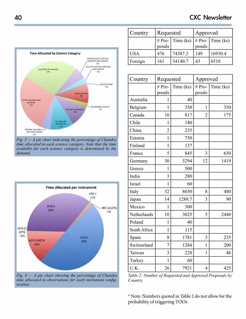
40 CXC Newsletter

Table 2: Number of Requested and Approved Proposals by Country

Country Requested Approved# Pro-posals

Time (ks) # Pro-posals

Time (ks)

USA 476 74387.2 149 16930.4Foreign 161 34140.7 43 6510

Country Requested Approved# Pro-posals

Time (ks) # Pro-posals

Time (ks)

Australia 1 40Belgium 1 350 1 350Canada 10 817 2 175Chile 1 140China 2 235Estonia 1 750Finland 1 137France 5 845 3 650Germany 30 5294 12 1419Greece 1 500India 3 280Israel 1 60Italy 32 8650 8 480Japan 14 1288.7 3 90Mexico 1 300Netherlands 10 3025 5 2440Poland 1 40South Africa 1 115Spain 8 1781 3 235Switzerland 7 1284 1 200Taiwan 3 228 1 46Turkey 1 60U.K. 26 7921 4 425

* Note: Numbers quoted in Table 2 do not allow for the probability of triggering TOOs

Fig. 6 — A pie chart showing the percentage of Chandra time allocated to observations for each instrument config-uration.

SOLAR  SYSTEM  <1%  

STARS  AND  WD  9%  

WD  BINARIES  AND  CV  2%  BH  AND  NS  BINARIES  

10%  

SN,  SNR  AND  ISOLATED  NS  

11%  

NORMAL  GALAXIES:  X-­‐RAY  POPULATIONS  

5%  

ACTIVE  GALAXIES  AND  QUASARS  

27%  

CLUSTERS  OF  GALAXIES  27%  

EXTRAGALACTIC  DIFFUSE  EMISSION  AND  SURVEYS  

5%  

GALACTIC  DIFFUSE  EMISSION  AND  SURVEYS  

3%  

Time  Allocated  by  Science  Category  

Fig. 5 — A pie chart indicating the percentage of Chandra time allocated in each science category. Note that the time available for each science category is determined by the demand.

41Spring, 2015

Einstein Postdoctoral Fellowship ProgramPaul Green

“The most beautiful experience we can have is the mysterious.”- Albert Einstein

Well then, black holes, dark energy, or relativis-tic magnetohydrodynamics are all beautiful! That's a sampler of what Einstein Postdoctoral Fellows study, supported by NASA for up to three years of research relevant to NASA missions in high energy or grav-itational astrophysics, or cosmology. Each year, we invite applications and convene a review committee who get to see what young cutting-edge researchers are interested in. This year, we received 148 applica-tions for 14 positions. That's a lower oversubscription than usual, due in part to a number of current Fellows taking faculty jobs! Applications were due by Novem-ber 7, 2014, and the selection panel met January 14, 2015. That same day, we contacted applicants to offer our congratulations or condolences, or for a few har-ried aspirants, their waitlist chances. The list of new 2015 Fellows is now confirmed. Their names, brief bios, and their Host Institutions can be seen at http://cxc.harvard.edu/fellows/.

Every year we convene an Einstein Fellows Sym-posium, which is a whirlwind of cool ideas, devilish puzzles, and ever more spectacular graphics, but also a shmoozefest for the Fellows. Abstracts, PDFs, and even video of the presentations from the symposium of October 2014 are available at http://cxc.harvard.edu/fellows/program_2014.html, and we look for-ward to another such exchange this coming Fall.

What have current Fellows been up to? Wen-fai Fong (2014, University of Arizona) received a 2014 Fireman Fellowship, awarded annually to a Harvard graduating student with the most impactful thesis in experimental astrophysics. Chris Nixon (2012, UC Boulder) accepted an STFC Ernest Rutherford Fel-lowship to the University of Leicester. Grant Tremblay (2014, Yale) had a press release (http://hubblesite.org/newscenter/archive/releases/2014/26/full/) about a string of “super star clusters” strung like pearls be-tween two massive ellipticals in a z ∼ 0.335 lensing cluster imaged by Hubble, Chandra, and soon ALMA. A NASA press release (http://svs.gsfc.nasa.gov/cgi-bin/details.cgi?aid=10082) highlighted the discov-ery by Laura Blecha of a powerful blue object 2,600 light years from the dwarf galaxy Markarian 177 that could be a black hole recoiling after a galaxy merg-er, or perhaps a very unusual type of star known as a Luminous Blue Variable. Rutger van Haasteren and his wife report, despite the ripples it will surely cause, the non-detection by gravitational wave detectors of a new baby boy.

This year, I took over the duties of Einstein Fel-lowship Program Scientist from Andrea Prestwich, who has ably shepherded and developed the program since 2010. Though faced with a steep learning curve, I haven't screwed anything up too badly. Yet. To my knowledge. One development we are all excited about is a new Einstein Fellows Alumni Mentorship Pro-gram. The breadth of experience amongst previous Fellows presents a wonderful opportunity for current Fellows to share their hopes, concerns, and strategies with others who have explored a variety of paths of mystery, beauty, and befuddlement.

Cost ProposalsPIs of proposals with US collaborators were in-

vited to submit a Cost Proposal, due in September 2014 at SAO. In Cycle 16, each project was allocated a budget based on the details of the observing pro-gram (see CfP Section 8.4). Awards were made at the allocated or requested budget levels, whichever was lower. The award letters were emailed in December, in time for the official start of Cycle 16 on 1 January 2015.

Proposal StatisticsStatistics on the results of the peer review for a

given cycle can be found on our website (http://cxc.harvard.edu/target_lists/index.html). We present a subset of those statistics here. Fig. 4 displays the ef-fective over-subscription rate for each proposal type as a function of cycle. Figs. 5, 6 show the percentage of time allocated to each science category and to each instrument combination. Table 2 lists the numbers of proposals submitted and approved per country of or-igin.

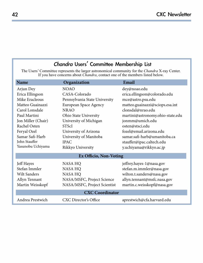
42 CXC Newsletter

Chandra Users’ Committee Membership ListThe Users’ Committee represents the larger astronomical community for the Chandra X-ray Center.

If you have concerns about Chandra, contact one of the members listed below.

NOAO dey@noao.eduCASA-Colorado erica.ellingson@colorado.eduPennsylvania State University mce@astro.psu.eduEuropean Space Agency matteo.guainazzi@sciops.esa.intNRAO clonsdal@nrao.eduOhio State University martini@astronomy.ohio-state.eduUniversity of Michigan jonmm@umich.eduSTScI osten@stsci.eduUniversity of Arizona fozel@email.arizona.eduUniversity of Manitoba samar.safi-harb@umanitoba.caIPAC stauffer@ipac.caltech.eduRikkyo University y.uchiyama@rikkyo.ac.jp

Name Organization Email

Ex Officio, Non-Voting

CXC Coordinator

NASA HQ jeffrey.hayes-1@nasa.govNASA HQ stefan.m.immler@nasa.govNASA HQ wilton.t.sanders@nasa.govNASA/MSFC, Project Science allyn.tennant@msfc.nasa.govNASA/MSFC, Project Scientist martin.c.weisskopf@nasa.gov

CXC Director’s Office aprestwich@cfa.harvard.edu

Arjun DeyErica EllingsonMike EracleousMatteo GuainazziCarol LonsdalePaul MartiniJon Miller (Chair)Rachel OstenFeryal OzelSamar Safi-HarbJohn StaufferYasunobu Uchiyama

Jeff HayesStefan ImmlerWilt SandersAllyn TennantMartin Weisskopf

Andrea Prestwich

43Spring, 2015

Date PI Objects Title

8 January Peter Maksym(University of Alabama) Abell 1795 Death by Black Hole in Small Galaxy?

27 January Neil Gehrels (GSFC) SN 2014J NASA Spacecraft Take Aim at Nearby Supernova

18 February Lucia Pavan (University of Geneva) IGR J11014-6103 NASA’s Chandra Sees Runaway Pulsar

Firing an Extraordinary Jet

5 March Rubens Reis (University of Michigan) RX J1131-1231 Chandra and XMM-Newton Provide Direct

Measurement of Distant Black Hole’s Spin

19 March CXC CXC Director Dr. Belinda Wilkes Chosen to Lead Chandra X-ray Center

2 April NASA/CXC Einstein Fellows 2014 Einstein Fellows Chosen

7 May Konstantin Getman(Penn State)

NGC 2024 & Orion Nebula Cluster

NASA’s Chandra Delivers New Insight into Formation of Star Clusters

24 June Esra Bulbul (CfA) Perseus Cluster Mysterious X-ray Signal IntriguesAstronomers

22 July NASA/CXC Chandra’s Anniversary NASA’s Chandra X-ray ObservatoryCelebrates 15th Anniversary

14 August Raffella Margutti (CfA) SN 2014J NASA’s Chandra Observatory Searches for Trigger of Nearby Supernova

16 September Ignazio Pillitteri (INAF) WASP-18 NASA’s Chandra X-ray Observatory Finds Planet That Makes Star Act Deceptively Old

27 October Irina Zhuravleva (Stanford University)

Perseus & Virgo Clus-ters

NASA’s Chandra Observatory Identifies Impact of Cosmic Chaos on Star Birth

13 November Yang Bai (University of Wisconsin) Galactic Center NASA X-ray Telescopes Find Black Hole

May Be a Neutrino Factory

18 December Paolo Tozzi (INAF) XDCP J0044.0-2033 NASA’s Chandra Weighs Most Massive Galaxy Cluster in the Universe

Links to all of these press releases can be found at: http://www.chandra.harvard.edu/press/14_releases/.

Additional image releases and other features that were issued during 2014 are available at:http://www.chandra.harvard.edu/photo/chronological14.html.

2014 CXC Press ReleasesMegan Watzke

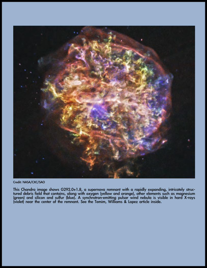
Credit: NASA/CXC/SAO

This Chandra image shows G292.0+1.8, a supernova remnant with a rapidly expanding, intricately struc-tured debris field that contains, along with oxygen (yellow and orange), other elements such as magnesium (green) and silicon and sulfur (blue). A synchrotron-emitting pulsar wind nebula is visible in hard X-rays (violet) near the center of the remnant. See the Temim, Williams & Lopez article inside.