change detection from heterogeneous data...

Change Detection From Heterogeneous DataSources

Tsuyoshi Ide

Abstract Detecting the changes in business situations is an important technicalchallenge. This chapter focuses onchange detectiontechnologies, including outlierdetection and change-point detection. In particular, we focus on how to handle theheterogeneous and dynamic features of the data in service businesses. We intro-duce a method of the singular spectrum transformation for change-point detectionin heterogeneous data. We also introduce a technique for proximity-based outlierdetection to handle dynamic　 data. Using real-world sensor data, we demonstratethe utility of the proposed methods.

1 Introduction

Recent advances in sensing and storage technologies are making it possible to col-lect and store real-valued time-series data in various domains. Examples of the datainclude POS (point-of-sales), biomarker, geospatio-temporal, etc. Unlike human-generated data such as call center text logs, analyzing real-valued time-series datais generally challenging, since the values of the sensors are not directly meaningfulin general, and the amount of data is often intractably huge.

For industrial domains such as transportation, manufacturing, energy & utilities,etc., where optimized operations of physical systems are at the heart of successfulbusiness, the effective use of sensor data is critical. For example, early detection of asystematic occurrence of defective products is essential to avoid potential losses. Wehave recently witnessed rapid changes towards service businesses in various indus-tries. Recent examples include system monitoring services for production systemsand construction equipment. Another example where the analysis of sensor data iscritical is location-based services, which are growing rapidly. To exploit geospatial

Tsuyoshi IdeIBM Research – Tokyo, 1612-14 Shimo-tsuruma, Yamato-shi, 242-8502 Kanagawa, Japan, e-mail:[email protected]

1

2 Tsuyoshi Ide

data, real-time position information needs to be analyzed by combining it with cer-tain data from individual products and consumers. All these examples clearly showthe need for practical methods for analyzing sensor data in service businesses.

In spite of the growing awareness of sensor data analytics for service businesses,little about this topic appears in the literature. This is possibly due to the fact thatknowledge discovery from noisy sensor data is quite difficult with traditional ap-proaches, and the problem settings can be quite different from traditional situations.Figuratively, traditional methods are capable of handling only a small percentage ofthe data, leaving the rest unused. This also means that practical new technologiescould lead to a major business advantage in the unexplored spaces, just as informa-tion retrieval techniques based on new disciplines of machine learning opened newdoors to business on the Internet.

In this chapter, we focus onanomaly detectiontechnologies, including the tasksof outlier detection and change-point detection. In particular, we focus on how tohandle the heterogeneous and dynamic data that is often collected by service busi-nesses. Toward this goal, we propose two new technologies. First, we introduce achange-point detection method calledsingular spectrum transformation(SST). Al-though traditional approaches to change-point detection consist of two separatedsteps, typically density estimation and scoring, SST unifies them to give a one-step algorithm with the aid of the mathematical theory called the Krylov subspacemethod. Thanks to the simplified structure of the algorithm, SST is quite robust toheterogeneities in the data.

Second, we propose a novel technique for proximity-based outlier detection. Inthis approach, we use a regularization technique to automatically discover modularstructures of the system. In other words, for each variable, the algorithm automat-ically finds a set of variables that are in proximity to the variable. The size of theproximity sets is automatically determined in accordance with the strength of reg-ularization. This feature is quite useful in heterogeneous systems, since how manyneighbors each variable has depends on the nature of each variable. Based on theproximity analysis, we compute the degree of outlier-ness in a probabilistic fashion.

Here is the structure of the chapter. In Section 2, we first review previous ap-proaches to anomaly detection, and then summarize the motivation behind our ap-proach. In Section 3, we describe the practical change-point detection method calledSST based on our previous work [13, 17]. In Section 4, we propose a novel outlierdetection method based on sparse structure learning. In Section 5, we briefly presentsome experimental results that demonstrate the utility of our methods. Finally, inSection 6, we summarize our results.

2 Previous work and our motivation

As mentioned in the introduction, sensor data has different features from traditionaldata such as that used in statistics and data mining. Except for cases in which wehave detailed knowledge of the internal structures of the systems, there are only

Change Detection From Heterogeneous Data Sources 3

a few options available. In practice, detecting signs of changes is perhaps the mostimportant task. The first half of this section reviews existing anomaly detection tech-niques and their limitations. For a more complete survey, see [5].

There are many scenarios for anomaly detection, depending on the perspectivesand the definitions of anomalies. In the data mining community, these scenariosappear in the literature:

• Outlier detection• Change-point detection• Discord discovery

We will give a brief description of each task in the following subsections. Inwhat follows, we assume that we are given a sequence in anM-dimensional vec-tor D ≡ {xxx(1),xxx(2), ...,xxx(N)} up to a discrete time pointN. By definition, xxx(n) =(x1

(n),x2(n), · · · ,xM

(n))>, and at each time point, which is assumed to be equi-interval, we observeM values from individual sensors. The superscript> representsthe transpose operation.

2.1 Outlier detection

Outlier detection looks at how much novelty a single sample reveals. Examplesinclude temperature monitoring of a chemical plant, where an alert must be raisedwhen an exceptionally high temperature is observed. In general, outlier detectionconsists of two steps:density estimationandscoring.

In the context of sensor data, density estimation is the same as creating a pre-dictive model, and the goal of this step is to find a probability densityp(xxx|D) thatpredicts the value of a newly observed sample, given the previous dataD . Thereare roughly two types of approaches for this step. One is based on density estima-tion techniques for i.i.d. (identically and independently distributed) samples, and theother is based on time-series prediction techniques. First we look at the i.i.d. modelsand time-series prediction methods are covered in the next subsection.

In statistics, a standard approach is to assume a Gaussian distribution:

N (xxx|µµµ ,Λ−1) =|Λ| 12

(2π)M2

exp

{−1

2(xxx−µµµ)>Λ(xxx−µµµ)

}. (1)

For the model parameters, the meanµµµ and the precision matrixΛ, are typicallydetermined using maximum likelihood. By using estimated parameters,µµµ andΛ, inthe model, we havep(xxx|D) = N (xxx|µµµ, Λ−1). Although the Gaussian is the simplestmodel for multivariate data, accurately estimatingΛ, which is defined as the inverseof the covariance matrixS, is challenging in practice, as explained below.

Based on this model, Hotelling’sT2-test is widely used as the standard techniqueof outlier detection [1]. The idea is to use the (squared) Mahalanobis distance

4 Tsuyoshi Ide

T2(xxx|µµµ ,Λ) = (xxx−µµµ)>Λ(xxx−µµµ)

as the measure of outlier-ness. Note thatT2 itself is a random variable givenxxx, sinceestimated values ofµµµ andΛ will not be perfect for finite training samples. In thisdefinition, the precision matrix represents the effect of heterogeneities of differentdimensions. Specifically, if one variable has a large variance (i.e. small precision),then the distribution should be stretched along the axis, giving an ellipsoidal distri-bution.

Although the Hotelling test is theoretically mature, in practice it is known toproduce many false alerts. This is because the set of assumptions behind the theoryare not fully satisfied. Problems that have been addressed to date in the literatureinclude:

1. Non-stationarity. The distribution may change over time.2. Multi-modality. The distribution consists of several clusters of densities.3. Numerical instability. If the dimensionality is high (M % 30) or collinear, then

the rank-deficiency makes it hard to invert the covariance matrix.

For the first and second problems, Yamanishi et al. [32] proposed using a se-quential parameter estimation algorithm for Gaussian mixtures. Although in theorythis approach seems useful to handle the problems of non-stationarity and multi-modality, their algorithm is known to be numerically unstable in practice. This be-cause estimation of a covariance matrix is much harder than expected especially forhigh dimensional systems. Breunig proposed a simpler and numerically stable ap-proach with a metric for outlier-ness called LOF (local outlier factor) [4]. AlthoughLOF was first introduced in an intuitive fashion, this metric amounts to an approxi-mation for the density estimation step, where ak-nearest neighbor (k-NN) heuristicis used in place of full density estimation. Thanks to the locality ofk-NN, LOF canin principle handle multi-modality. However, again, the intuitive notion of LOF doesnot necessarily work with many dimensions, where, due to the curse of dimension-ality, all of the samples are necessarily very close to each other. Also, choosing anoptimalk requires a heuristic approach. In addition, thek-NN approach is memoryintensive since all of the previous samples must be available.

For the third problem, numerical instability, which is essentially due to thegap between the nominal and intrinsic dimensionalities, there are at least two ap-proaches. The first approach isdimensionality reduction, which focuses on a sub-space where the redundant dimensions are ignored. One of the earliest work in thisdirection in the context of anomaly detection is [14], where the use of PCA (prin-cipal component analysis) was proposed to detect anomalies in computer networks.The second approach involves the use ofregularization. In Section 4, we explainhow useful it is in outlier detection.


2.2 Change-point detection

Change-point detection is the problem of detecting structural changes in the datageneration mechanism behind observed data. For example, one might want to raisean alert when the system starts producing unusual vibrations even if the variablesare within standard ranges.

Unlike outliers, change-points can take various forms, such as cusps, steps,changes in frequency, etc. A general-purpose approach is to learn a generative modelfor the data based on previous recordings, and compute the degree of goodness offit for the model with the present data. If the goodness of the model is sufficient forthe present data, we determine that a change is occurring in the system [3].

In this procedure, there are two steps in change-point detection:density estima-tion andscoring. In the first step, we try to find a generative model based on recently

observed data. Letw be the size of window along the time axis, and letD(t)w be a

notation for{xxx(t−w+1), xxx(t−w+2), ..., xxx(t)}. Our first step is to find the probability

function that best fits the recent dataD(t)w for the modelp(xxx|D). For the next scor-

ing step, the likelihood ratio is a basic metric for scoring the degree of change:

z(t)≡ ∑xxx∈D(t)

w

lnp(xxx|D (t)

w )

q(xxx), (2)

whereq(·) represents a baseline distribution. In practical scenarios,q(·) is oftenthought of as the distribution under the normal situation. In this case, the likelihoodratio is a metric of the faultiness of the system．

For a single variable that is Gaussian-distributed around a constant value, amethod called CUSUM (cumulated summation) is well-known as a baseline methodfor change-point detection [3]. If the Gaussian assumption is allowed, the likeli-hood ratio has a number of desirable properties with Chi-squared distribution andNeyman-Pearson optimality [1]. However, as expected, in most cases in sensor dataanalytics, its utility is quite limited due to the dynamic and non-stationary nature ofthe systems.

To tackle the problems in traditional approaches, there are three prominent andrecent approaches to change-detection in the data mining community. The first ap-proach, which is perhaps the most similar to the traditional statistical analysis, isbased on direct estimation of the density ratio [20]. In this approach, rather thanseparately estimating the densities of the numerator and denominator, the likelihoodratio is directly modeled and estimated using a kernel method. For details, see [28].

In the second approach, a time-series prediction model is estimated rather thanusing i.i.d. models to handle the dynamic nature of the data. One of the earliest de-scriptions includes [31], where a sequential update algorithm is proposed for fittingan AR (auto-regressive) model. We can focus on the simplest case ofM = 1 forsimplicity. The AR model of orderm is defined as

p(x(t)|aaa,b) = x(t−1)a1+x(t−2)a2+ · · ·+x(t−m)am+b,

6 Tsuyoshi Ide

whereaaa ∈ Rm andb ∈ R1 are parameters to be estimated from the data in a se-quential fashion. As is well-known, the AR model assumes a specific periodicitythroughm, the order of the AR model. This means that the AR model is not capableof handling non-stationary dynamics. One approach to this problem is to introducea latent state into the model. The earliest work in this direction includes the methodof SST [13, 17], and its theoretical analysis was given in [21], which shows a clearrelationship between SST and system identification of state-space models. In a latersection, we will revisit this point.

Finally, in the third but maturing approach, the task of change-point detection istreated as a model selection problem [30, 29]. This is a new and interesting researcharea, where the practical requirements interact with deep theoretical analysis.

2.3 Discord discovery

So far we have looked at approaches explicitly based on probabilistic methods. Inaddition, algorithmic approaches are also popular in the data mining community.One of the typical tasks in the present context isdiscord discovery. In this task,the time series data is first transformed into a set of subsequences, and then eachsubsequence is checked to see if it is far from the average behavior. This type ofapproach is practically useful in some applications. For example, if an unusual pulsepattern is found in the time-series data of an ECG (electro-cardiogram), it may bean indication of a heart attack [22]．

Let us consider the simplest case ofM = 1 for simplicity. Letw be the size ofthe sliding windows. Usingw, we transform the data into a set of subsequences{sss(w),sss(w+1), ...,sss(N)}, where

sss(t) ≡ (x(t−w+1), x(t−w+2), ..., x(t))> (3)

is a subsequence represented as a vector in aw-dimensional space. Adiscord isdefined as an outlier in the set of subsequences. As metrics of the outlier-ness, themean and median of thek-NN distances are often used. In this approach, one needsto compute thek-NNs for each sample, which is computationally expensive andmemory intensive. To address these limitations, several heuristics have been pro-posed [33].

In the data mining community, the task of discord discovery (and closely relatedtask of motif discovery) is often handled with a technique called SAX [22]. SAX isa data compression method that converts real-valued time series into discrete sym-bols. After the conversion, a number of useful techniques in discrete mathematicssuch as dynamic programming can be used. However, the optimality of the sym-bolic representations has not been deeply addressed in the literature to date. Thisis an interesting research topic, which calls for a combination with probabilisticapproaches [11].


One subtle problem in the sliding window approach is that the overlap betweenneighboring windows may cause pathological phenomena such as sinusoidal effectsin the subsequence time-series clustering [24, 12]. How to avoid such effects isanother interesting research topic [8].

2.4 Goal of this chapter

As mentioned, outlier detection and change-point detection are traditional problemsettings in statistics for anomaly detection. However, methods developed in statisticsare known to be of limited effectiveness in practice in many cases. A typical exam-ple is asymptotic theories. In modern sensor data that can be dynamic and noisy, thenumber of samples is almost infinite along the time axis. Therefore it is sometimesthe case that the confidence interval derived from an asymptotic distribution can betoo narrow to produce a reasonable false positive rate. These types of difficultiesare well-known in such tasks as FDC (fault detection and classification) in semicon-ductor manufacturing processes. Therefore recent research focus has been on newlydeveloped approaches in the data mining and machine learning communities.

This chapter covers these new approaches to anomaly detection from two per-spectives. First we look at SST for change-point detection. As mentioned in the in-troduction, SST has the unique feature that the density estimation and scoring stepsare unified. As a result, we can avoid numerically unstable parameter estimation.Although SST relies on SVD (singular value decomposition) that is usually com-putationally expensive, we will show our algorithm based on the Krylov subspacemethod allows overcoming this issue.

Next we propose a novel method for outlier detection, which is based on sparsestructure learning of the graphical Gaussian model (GGM). Our method has a num-ber of advantages over existing methods. First, our algorithm is numerically stablethanks to a regularization technique. Second, the sparse structure learning providesinsights into the system. Identifying a sparse structure between variables amountsto looking at an essential relationship between those variables. More importantly,thanks to the sparseness, we can automatically find modular or cluster structureswithin the system. Finally, based on the modular structure, our algorithm is capa-ble of doinganomaly localization[16, 15, 18]. This means that, forM-dimensionaltime series, our output isM anomaly scores for a single sample, rather than a singlescalar. This is a very important feature in practice, since we can easily come up witha response for a detected anomaly once we know which variables are responsiblefor the fault.

8 Tsuyoshi Ide

3 Change-point detection

Before getting into the details of the algorithm, let us first look at an motivating ex-ample of change-point detection in heterogeneous systems [13]. The essence of ouridea is illustrated in Fig. 1, where two artificially generated data sets and their SSTsare shown. While it is difficult to infer any relationship between the two originalvariables, SST clearly reveals a hidden relationship involving the synchronizationof their change points. Note that the results in Fig. 1 (b) and (d) were obtained usinga common algorithm and a shared parameter set, so we see that, by performing SST,the problem of data mining in heterogeneous systems can be reduced to those of ho-mogeneous problems without using any detailed knowledge about the behavior ofdata. The notion ofchange-point correlation[13] is indeed a key idea for knowledgediscovery from dynamic systems that are strongly-correlated and heterogeneous.

change-point score

change-point scoreapparentlydifferent

Similar

time

time

(d)

(c)

(b)

(a)

0 100 200 300 400 5000

0.020.040.06

0 100 200 300 400 5000

0.020.040.06

Fig. 1 Example of SST in a heterogeneous system. The original time-series in (a) and (c) are trans-formed into change-point scores in (b) and (d), revealing a hidden similarity. Clear synchronizationof the two change points suggests a causal relationship between the two variables.

3.1 Overview of the SST algorithm

For clarity in the presentation, let us consider a one-dimensional time-series{x(t) ∈R | t = 1,2, ...}. We are given a subsequence of lengthw as Eq. (3) (We assume that


t time

Fig. 2 Overview of SST.

the data points are collected at constant intervals). At each timet, letH1 andH2 bematrices containingn subsequences defined as

H1(t)≡[sss(t−n), ...,sss(t−2),sss(t−1)]

H2(t)≡[sss(t−n+ γ), ...,sss(t−1+ γ)],

whereγ is a positive integer. Fig. 2 shows an example where three subsequences aretaken both in the vicinity of the present time and in the past.

The column space ofH1(t), the space spanned by the column vectors, should con-tain the information about the patterns appearing in the past domain of the time se-ries. The SST uses the principal components as typical representative patterns of thecolumn space: Find ther (<w,n) top left singular vectors ofH1(t), uuu(1),uuu(2), ...,uuu(r).We assume these are orthonormal. Hereafter, we omit the argumentt unless confu-sion is likely. Let the subspace spanned by these vectors be

Hr ≡ span{uuu(1),uuu(2), ...,uuu(r)}. (4)

Similarly, we can get the representative patterns around the present timet byperforming the SVD ofH2. We use the top principal componentµµµ of H2 as therepresentative pattern.

We define the change-point (CP) scorez at timet as

z≡ 1−r

∑i=1

K(i,µµµ)2, (5)

which can be interpreted as the distance between the subspaces. Since it is empiri-cally true that the score is not very sensitive to the choices ofn andγ [13], we setn=w andγ =w/2. Forw, a value less than 100 typically works well. An appropriatepreprocess (e.g. down-sampling) can be used to adjustw to this range. Empirically,a value of three or four works well forr even whenw is on the order of 100.

10 Tsuyoshi Ide

3.2 Introducing Krylov subspace

By definition, the singular vectorsuuu(i) are in the column space ofH1. Instead ofusing the full column space, we attempt to use ak-dimensional subspaceVk, andthus reduce the original eigen problem to ak× k matrix problem (assumingr <k < w). Notice that what we want is not singular vectors themselves but the innerproduct w.r.t. a given vectorµµµ .

Imagine that we havek orthonormal bases representing such a subspace:{qqq1, ...,qqqk},and we approximate each of the singular vectoruuu(i) as

uuu(i) 'k

∑α=1

b(i)α qqqα , (6)

whereb(i)α is a coefficient that is assumed to be unknown at this point. Since our goalis to compute the overlap withµµµ and there is arbitrariness in the choice of the basesin the subspace, we assume

qqq1 = µµµ ,

which is always possible. Because of the orthogonality of theqqqαs and the fact thatqqq1 = µµµ , computingµµµ>uuu(i) can be reduced to taking the first element of thebbb(i)s.Explicitly, the kernel function is approximated by

K(i,µµµ)'k

∑α=1

b(i)α µµµ>qqqα = b(i)1 , (7)

which means thatthe inner product can be computed directly from the k-dimensionalvectors bbb(i)s without explicitly using the uuu(i)s.

Now our remaining problem is how to findVk and the coefficient vectorsbbb(i). Tofind Vk, let us consider this problem:Given an s-dimensional subspaceVs⊂ Rw, construct a subspaceVs+1 by adding avector toVs so that the increase of the overlap betweenVs+1 and{uuu(1), ...,uuu(s)} ismaximized.

Let us start withV1 spanned byµµµ . Recall that finding the left singular vector forH1 is equivalent to the eigen problem ofC ≡ H1H1

>, and the eigen equation forC is equivalent to the maximization problem of the Rayleigh quotient [9], which isdefined by

R(uuu) =uuu>Cuuuuuu>uuu

.

To satisfy the requirement, when we constructV2 = span{µµµ ,∆∆∆} by adding∆∆∆ ∈Rw,the added vector should contain the steepest ascent direction ofR given by

dduuu

R(uuu)

∣∣∣∣uuu=µµµ

=−2

µµµ>µµµ[R(µµµ)µµµ−Cµµµ ] .

Thus, if we chooseCµµµ as∆∆∆ , span{µµµ ,Cµµµ} contains this steepest direction.


Continuing this procedure, we see that ak-dimensional space

Vk(µµµ ,C)≡ span{µµµ,Cµµµ, ...,Ck−1µµµ}

is the bestk-dimensional subspace in terms of maximization ofR, givenµµµ . In otherwords, there are many choices of ak-dimensional subspace over the entire columnspace ofH1, but among all of the choices, the subspace that has the largest weight ofuuu(1), ...,uuu(r) isVk(µµµ ,C), under the constraint thatµµµ is the starting base. In mathemat-ics, Vk(µµµ ,C) is called theKrylov subspaceinduced byµµµ andC [9]. Alternatively,one may say thatµµµ is theseedof the Krylov subspace.

3.3 Fast computation ofz

Let us consider our next question: how to find the coefficient vectorsbbb(i). Beforedirectly consideringbbb(i), let us consider how to find the orthonormal set{qqq1, ...,qqqk}.This is an easy task, since, givenVk(µµµ,C) ≡ span{µµµ,Cµµµ, ...,Ck−1µµµ}, we can useGram-Schmidt orthogonalization starting fromµµµ to produce the orthonormal set.Note that the Gram-Schmidt orthogonalization is essentially equivalent to the QRfactorization of

Vk(µµµ ,C)≡[µµµ,Cµµµ , ...,Ck−1µµµ

],

which is called the Krylov matrix. Fortunately, in the QR factorization of the Krylovmatrix, a special and helpful property holds (for proof, see [9]):

Theorem 1 The orthogonal matrixQk ≡ [qqq1, ...,qqqk] ∈ Rw×k given by the QR fac-torization ofVk(µµµ ,C) tridiagonalizesC.

This theorem says thatQ>k CQk is a tridiagonal matrix. What is this matrix? Tosee it, note that Eq. (6) can be written as

uuu(i) 'k

∑α=1

b(i)α qqqα = Qkbbb(i).

Then the eigen equation forC, which is equivalent to SVD ofH1, is rewritten as

Q>k CQkbbb= λbbb. (8)

This means that we can directly find the coefficient vectors{bbb(1), ...,bbb(r)} by diago-nalizing a tridiagonal matrixTk ≡ Q>k CQk.

Let α1, ...,αk andβ1, ...,βk−1 be the diagonal and subdiagonal elements ofTk. Ifwe consider thes-th column of the equationCkQk = QkTk, it follows that

Cqqqs = αsqqqs+βs−1qqqs−1+βsqqqs+1,

12 Tsuyoshi Ide

whereqqqs is thes-th column vector ofQk. Using the orthogonal relationqqq>i qqq j = δi, j ,we immediately haveαs = qqqs

>Cqqqs. In this way, it is easy to construct an algorithmto find αs andβs sequentially from this recurrent equation:

Subroutine 1 Lanczos( C,µµµ ,k) InputC ∈Rw×w, µµµ ∈Rw, and a positive integerk (< w). Initialize as rrr0 = µµµ , β0 = 1, qqq0 = 0, and s= 0. Repeat

qqqs+1 = rrrs/βs

s← s+1αs = qqqs

>Cqqqsrrrs = Cqqqs−αsqqqs−βs−1qqqs−1βs = ||rrrs||

until s= k. Return{α1, ..,αk} and{β1, ..,βk−1}.By running this procedure up tok<w, we obtainTk (=Q>k CQk) directly. Notice

that we donot need to explicitly computeqqq1, ...,qqqk. This tridiagonalization proce-dure is called the Lanczos algorithm.

Finally, the CP score is computed using Eqs. (5) and (7) as

z' 1−r

∑i=1

x(i)2. (9)

Notice that we do not at all need to explicitly compute either theuuu(i)s or the innerproduct. We call this implicit kernel calculation based on Krylov subspace learningthe implicit Krylov approximation(IKA).

Our fast SST algorithm is summarized as:

Algorithm 1 (IKA-SST) At each t, do

1. Computeµµµ as the SVD ofH2.2. α1, ..,αr ,β1, ..,βk−1← Lanczos( C,µµµ,k) .3. Compute the r top eigenvectors of the tridiagonal matrixTk.4. Compute the CP score using Eq. (9).

For the dimension of the Krylov subspaceVk(µµµ ,C), one reasonable choice is

k=

{2r r ∈ even2r−1 r ∈ odd

. (10)

The rationale of this rule is that the Krylov subspace is also the best subspace for thesmallest eigenstates as well as for the largest eigenstates [9], sok should be abouttwice r. Note that the IKA is independent of the choice of the SST-native parametersn andγ.

3.4 Relationship to subspace identification method

The SVD approach for the SST is similar to the subspace identification methodin control theory [25]. This is indeed the case, and the equivalence between them


was theoretically explored by Kawahara [20]. This work showed that SST can bethought of as an approximated version of the subspace identification algorithm todetermine the system parameters of a state-space model. This suggests that SST hasa unique feature that unifies the previous sequential AR model approach [31] into asingle, computationally efficient framework. Due to space limitations, however, wewill discuss this in a separate paper.

4 Proximity-based outlier detection

This section proposes a new outlier detection method based on sparse structurelearning. We first consider how to learn a sparse structure from the data. We as-sume thatD has been standardized to have zero mean and unit variance. Then thesample covariance matrixS is given by

Si, j ≡1N

N

∑n=1

x(n)i x(n)j , (11)

which is the same as the correlation coefficient matrix for this data.The use of sparse structure learning in anomaly detection was first proposed

in [15]. While the work [15] addresses an anomaly scoring problem in a settingsimilar to two-sample test in statistics, we extend their framework to include outlierdetection by considering a conditional probability function.

4.1 Penalized maximum likelihood

In the GGM, structure learning is reduced to finding a precision matrixΛ for themultivariate Gaussian (Eq. (1)). If we do not consider any regularization for now,we can getΛ by maximizing the log-likelihood

lnN

∏t=1

N (xxx(t)|000,Λ−1) = const.+N2{lndet(Λ)− tr(SΛ)} ,

where tr represents the matrix trace (sum over the diagonal elements), and we used

the well-known identityxxx(t)>

xxx(t) = tr(xxx(t)xxx(t)>) and Eq. (11). If we use the well-

known formulas for matrix derivatives

∂∂Λ

lndet(Λ) = Λ−1,∂

∂Λtr(SΛ) = S, (12)

then we readily obtain the formal solutionΛ= S−1. However, as mentioned before,this produces less practical information on the structure of the system, since the

14 Tsuyoshi Ide

sample covariance matrix is often rank deficient and the resulting precision matrixwill not be sparse in general.

Therefore, instead of the standard maximum likelihood estimation, we solve anL1-regularized version of the maximum likelihood:

Λ∗ = argmaxΛ

f (Λ;S,ρ), (13)

f (Λ;S,ρ)≡ lndetΛ− tr(SΛ)−ρ||Λ||1, (14)

where||Λ||1 is defined as∑Mi, j=1 |Λi, j |. Thanks to the penalty term, many of the en-

tries inΛ will be exactly zero. The penalty weightρ is an input parameter, whichworks as a threshold below which correlation coefficients are thought of as zero, asdiscussed later.

4.2 Graphical lasso algorithm

Since Eq. (13) is a convex optimization problem [2], one can use subgradient meth-ods to solve it. Recently, Friedman, Hastie, and Tibshirani [7] proposed an efficientsubgradient algorithm named graphical lasso. We recapitulate it in this subsection.

The graphical lasso algorithm first reduces the problem Eq. (13) to a series ofrelated L1-regularized regression problems by utilizing a block coordinate descenttechnique [2, 6]. Using the formula Eq. (12), we see that the gradient of Eq. (13) isgiven by

∂ f∂Λ

= Λ−1−S−ρ sign(Λ), (15)

where the sign function is defined so that the(i, j) element of the matrix sign(Λ) isgiven by sign(Λi, j) for Λi, j 6= 0, and a value∈ [−1,1] for Λi, j = 0.

To use a block coordinate descent algorithm for solving∂ f/∂Λ= 0, we focus ona particular single variablexi , and partitionΛ and its inverse as

Λ=

(L llllll> λ

), Σ≡ Λ−1 =

(W wwwwww> σ

), (16)

where we assume that rows and columns are always arranged so that thexi-related entries are located in the last row and column. In these expressions,W,L ∈R(M−1)×(M−1), λ ,σ ∈R, andwww, lll ∈RM−1. Corresponding to thisxi-based partition,we also partition the sample covariance matrixS in the same way, and write it as

S=

(S\i ssssss> si,i

). (17)

Now let us find the solution of the equation∂ f/∂Λ = 0. SinceΛ must be posi-tive definite, the diagonal elements must be strictly positive. Thus, for the diagonalelements, the condition of the vanishing gradient leads to


σ = si,i +ρ. (18)

For the off-diagonal entries represented bywww and lll , the optimal solution underwhich all the other variables are hold constant is obtained by solving

minβββ

{12||W

12 βββ −bbb||2+ρ ||βββ ||1

}= 0, (19)

whereβββ ≡W−1www, bbb≡W−1/2sss, and||βββ ||1 ≡ ∑l |βl |. For the proof, see [15]. Thisis an L1-regularized quadratic programming problem, and again can be solved effi-ciently with a coordinate-wise subgradient method [7].

Now to obtain the final solutionΛ∗, we repeatedly solve Eq. (19) forx1,x2, ...,xM,x1, ...until convergence. Note that the matrixW is full rank due to Eq. (18). This suggeststhe algorithm is numerically stable. In fact, as shown later, it gives a stable andreasonable solution even when some of the variables are highly correlated.

4.3 Connection to Lasso

The coordinate-wise optimization problem (Eq. (19)) derived by the graphical lassoalgorithm has a clear similarity to the lasso-based structure learning algorithm. Thealgorithm of Ref. [26] solves separate lasso regression problems for eachxi :

minβββ

{12||Ziβββ −yyyi ||2+µ ||βββ ||1

}, (20)

where we definedyyyi ≡ (x(1)i , ...,x(N)i )> and a data matrixZi ≡ [zzz(1)i , ...,zzz(N)

i ]> with

zzz(n)i ≡ (x(n)1 , ..,x(n)i−1,x(n)i+1, ...,x

(n)M )> ∈ RM−1.

Using the definition ofS (Eq. (11)), it is easy to see that this problem is equivalentto Eq. (19), when

W = S\i and ρ ∝ µ (21)

are satisfied. SinceW is a principal submatrix ofΛ−1, we see that there is a corre-spondence betweenW andS\i whenρ is small. It will never be satisfied forρ > 0,however. In this sense, the graphical lasso algorithm solves an optimization problemsimilar to but different from the one in [26]. This fact motivates us to empiricallystudy the difference between the two algorithms as shown in the next section.

16 Tsuyoshi Ide

4.4 Choosingρ

So far we have treated the penalty parameterρ as a given constant. In manyregularization-based machine learning methods, how to choose the penalty parame-ter is a subtle issue. In the present context, however,ρ should be treated as an inputparameter since our goal is not to find the “true” structure but to reasonably selectthe neighborhood.

To gain insight on how to relateρ with the neighborhood size, we note this result:

Proposition 1 If we consider a2×2 problem defined only by two variables xi andx j (i 6= j), the off-diagonal element of the optimalΛ as the solution to Eq.(13) isgiven by

Λi, j =

{− sign(r)(|r|−ρ)

(1+ρ)2−(|r|−ρ)2 for |r|> ρ0 for |r| ≤ ρ,

where r is the correlation coefficient between the two variables.

For the proof, see [15].Although this is not the solution to the full system, it gives us a useful guide

about how to chooseρ. For example, if a user wishes to think of any dependenciescorresponding to absolute correlation coefficients less than 0.5 as noise, then theinput ρ should be less than the intended threshold, and possibly a value aroundρ = 0.3 would work. If ρ is close to 1, the resulting neighborhood graphs will bevery small, while a value close to 0 leads to an almost complete graph where all ofthe variables are thought of as being connected.

We should also note that sparse structure learning allows us to conduct neigh-borhood selection in an adaptive manner. If a variable is isolated with almost no de-pendencies on other variables, then the number of selected neighbors will be zero.Also, we naturally expect that variables in a tightly-connected cluster would selectthe cluster members as their neighbors. We will see, however, that the situationswhen there are highly correlated variables are much trickier than they seem.

4.5 Outlier score

Now that a complete probabilistic model has been defined, let us proceed to the nextstep. Here we define the anomaly score for thei-th variable as

zi(xxx|Λ)≡− ln p(xi |x1, ..,xi−1,xi+1, ...,xM,Λ). (22)

Note that we haveM scores, corresponding to individual variables, for a single ob-servationxxx. The definition tells us the discrepancy between the value of thei-thvariable and its expected value given surrounding variables. Thanks to the sparse-


ness, the surrounding variables should be in the same module or cluster of thei-thvariable.

Since the right hand side of Eq. (22) is Gaussian, we can analytically write downthe expression. For example, for the first variable, the conditional distribution is

p(x1|x2, · · · ,xM) = N

(x1

∣∣∣∣∣− 1Λ1,1

M

∑i=2

Λ1,i xi ,1

Λ1,1

),

and the score is given as

s1≡12

ln2π

Λ1,1+

12Λ1,1

(M

∑i=1

Λ1,i xi

)2

. (23)

Putting together theM scores into a single vectorial expression, we get the finalresult of the outlier scores as

sss≡ sss0+12

diag(ΛxxxD−1xxx>Λ),

whereD≡ diag2(Λ) and

(sss0)i ≡12

ln2πΛi,i

.

5 Experiment

This section presents experimental results for the two anomaly detection methodsintroduced in the previous sections: IKA-SST for change-point detection, and theproximity-based outlier detection.

5.1 Parameter dependence of SST

An example of SST was already shown in Fig. 1. The time series (a) was generatedusing three linear functions with slopes of 1/300, 0, and−1/200. The other time-series (c) was generated using a sine functionx(t) = sin(2πt/λ ), for λ =

√80,√

120, and√

70. In (c), we also added random fluctuations to the amplitude and theperiods of up to±7.5% and±0.5%, respectively, to simulate fluctuations in realisticobservations. For both data sets, the change points are located att = 150 and 300.The results of SST in Figs. 1 (b) and (d) were calculated withw = 20 andr = 3.No IKA approximation was used. In spite of the apparent differences in the originaldata, we see that SST strikingly reveals the similarities without any ad hoc tuningfor individual time series. Existing methods such as differentiation [10] and wavelet-

18 Tsuyoshi Ide

based approaches [19] fail to detect the change points if a common parameter set isused for both sets.

The dependence onw is of particular interest in SST. We calculated SST as afunction of w for r = 3. The results are shown in Fig. 3. It is surprising that theessential features remain unchanged over a very wide range ofw, 6. w. 40, whilethe widths of the major features become broader asw increases. This robustness isquite advantageous for heterogeneous systems.

050

100150

200250

300350

400450

6

12

18

24

30

360

0.05

0.1

0.15

0.2

0.25

0.3

change-poin

t score

time

w

(a)

050

100150

200250

300350

400450

6

14

22

30

3800.020.040.060.080.10.120.140.160.180.2

change-poin

t score

time

w

(b)

Fig. 3 The dependence of SST onw for (a) the linear function and for (b) the oscillatory functionshown in Fig. 1 (a) and (c), respectively.


Table 1 Tested methods.

# symbol µµµ feedback{uuu(i)} kernel1 OI power no OI explicit2 EM EMPCA no EMPCA explicit3 OI FB power yes OI explicit4 EM FB EMPCA yes EMPCA explicit5 IKA power yes - implicit

0 1000506070

0 1000

40506070

0 10000

100200300

0 10000

50100150

0 10000

100200300

0 1000

0

200

400

0 1000

0

200

400

0 100052

56

60

(a) X_Acc

(b) Y_Acc

(c) Light1

(d) Light2

(e) Touch

(f) Microp1

(g) Microp2

(h) Temp

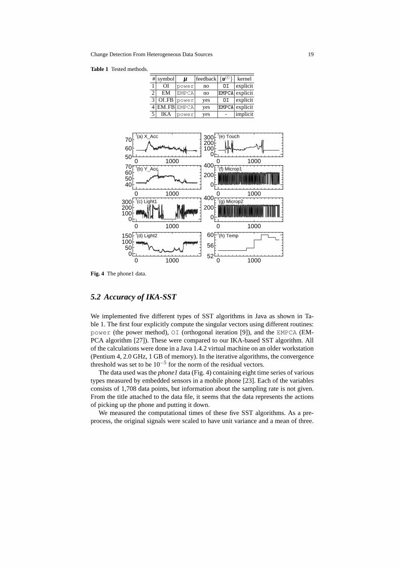
Fig. 4 The phone1 data.

5.2 Accuracy of IKA-SST

We implemented five different types of SST algorithms in Java as shown in Ta-ble 1. The first four explicitly compute the singular vectors using different routines:power (the power method),OI (orthogonal iteration [9]), and theEMPCA(EM-PCA algorithm [27]). These were compared to our IKA-based SST algorithm. Allof the calculations were done in a Java 1.4.2 virtual machine on an older workstation(Pentium 4, 2.0 GHz, 1 GB of memory). In the iterative algorithms, the convergencethreshold was set to be 10−5 for the norm of the residual vectors.

The data used was thephone1data (Fig. 4) containing eight time series of varioustypes measured by embedded sensors in a mobile phone [23]. Each of the variablesconsists of 1,708 data points, but information about the sampling rate is not given.From the title attached to the data file, it seems that the data represents the actionsof picking up the phone and putting it down.

We measured the computational times of these five SST algorithms. As a pre-process, the original signals were scaled to have unit variance and a mean of three.

20 Tsuyoshi Ide

110100100010000100000

10 25 50 75 100 250window sizetotal calc. time [s] 1: OI, 2: EM, 3: OI_FB, 4: EM_FB, 5: IKA1 2 3 45

Fig. 5 Total computation time of SST.

We imposed a periodic boundary condition on the data in performing SST. This iswas keep the number of data points the same over different values ofw. We used(r,k) = (3,5).

Figure 5 compares the computational times of the different algorithms on a loga-rithmic scale, averaged over five trials. We see that the improvement with the IKA-SST is drastic. It is about 50 times faster than the conventional SST methods foreachw.

Notice that this was accomplished with no significant approximation error. Toshow this, Fig. 6 compares the CP scores between EM and IKA forw = 50. Asshown, the overall fit between the EM and IKA results is very good, although thereare a few peaks which are not reproduced by IKA as indicated in Figs. 6 (b) and (g).Again, it is surprising that the IKA almost perfectly reproduces the results of EM,since IKA solves only 5× 5 problems while EM performs the complete SVD for50×50 matrices.

5.3 Outlier detection: hot box detection

We used the proximity-based anomaly detection method with a real problem in therail road industry. The task is often called hot box detection, where the goal is todetect anomalously behaving wheel axles based on temperature recordings. Undernormal operations, the temperature of an axle is expected to be highly correlatedwith the temperature of the other axles. Thus the proximity-based outlier detectionis useful in this application.

In contrast with obvious faults that are easily detected by a temperature thresh-old, detecting subtle signs of correlation anomalies is generally challenging. This


0 1000

0 1000

0 1000

0 1000

0 1000

0 1000

0 1000

0 1000

(a) X_Acc

(b) Y_Acc

(c) Light1

(d) Light2

(e) Touch

(f) Microp1

(g) Microp2

(h) Temp

EM

IKA

EMIKA

EMIKA

EMIKA

EMIKA

EM

IKA

EMIKA

EM

IKA

Fig. 6 CP score of the phone1 data (w= 50, r = 3).

is mostly because the temperature measurements are quite sensitive to externalwhether conditions. For example, the temperatures on rainy days are more than 10degrees lower than those on sunny days. Also, the temperatures of the first and thelast cars exhibit considerably different behaviors from the other cars.

We tested our outlier detection method, and compared the performance with astate-of-the-art method created by domain experts using extensive domain knowl-edge. The results were quite encouraging. Our method was several times better in adetection power, which is defined for a truly faulty axlei as

1σi[si(xxx)−〈si〉].

Here〈si〉 andσi are the mean and the standard deviation of thei-th outlier scoreover all of the samples, whilesi(xxx) is the outlier score of the faulty sample.

6 Summary

We have discussed approaches to anomaly detection for sensor data. We first re-viewed existing methods and their limitations. We then described two new ap-proaches to anomaly detection that are capable of handling heterogeneous variables.

22 Tsuyoshi Ide

First we gave a fast change-point detection method called IKA-SST. Thanks tothe robustness of SVD, this approach has a remarkable feature that no parametertuning is needed to handle heterogeneities of the variables. Second, we presenteda proximity-based outlier detection method, which has a very useful feature forautomatic discovery of the modular structure of a system. Finally, we showed someexperimental results for these methods.

References

1. T. W. Anderson.An Introduction to Multivariate Statistical Analysis. Wiley-Interscience, 3rd.edition, 2003.

2. O. Banerjee, L. E. Ghaoui, and G. Natsoulis. Convex optimization techniques for fitting sparseGaussian graphical models. InProc. Intl. Conf. Machine Learning, pp. 89–96. Press, 2006.

3. M. Basseville and I. Nikiforov.Detection of Abrupt Changes. Prentice Hall, Englewood Cliffs,New Jersey, 1993.

4. M. M. Breunig, H.-P. Kriegel, R. T. Ng, and J. Sander. LOF: identifying density-based localoutliers.ACM SIGMOD Record, 29(2):93–104, 2000.

5. V. Chandola, A. Banerjee, and V. Kumar. Anomaly detection: A survey.ACM ComputingSurvey, 41(3):1–58, 2009.

6. J. Friedman, T. Hastie, H. Hofling, and R. Tibshirani. Pathwise coordinate optimization.An-nals of Applied Statistics, 1(2):302–332, 2007.

7. J. Friedman, T. Hastie, and R. Tibshirani. Sparse inverse covariance estimation with the graph-ical lasso.Biostatistics, 9(3):432–441, 2008.

8. R. Fujimaki, S. Hirose, and T. Nakata. Theorectical analysis of subsequence time-series clus-tering from a frequency-analysis viewpoint. InProc. SIAM Intl. Conf. Data Mining, pp. 506–517, 2008.

9. G. H. Golub and C. F. V. Loan.Matrix computations (3rd ed.). Johns Hopkins UniversityPress, Baltimore, MD, 1996.

10. S. Hirano and S. Tsumoto. Mining similar temporal patterns in long time-series data and itsapplication to medicine. InProc. 2002 IEEE International Conference on Data Mining, pp.219–226, 2002.

11. B. Hu, T. Rakthanmanon, Y. Hao, S. Evans, S. Lonardi, and E. Keogh. Discovering the in-trinsic cardinality and dimensionality of time series using mdl. InProc. of the 11th IEEE Intl.Conf. on Data Mining (ICDM 11), 2011.

12. T. Ide. Why does subsequence time-series clustering produce sine waves? InProc. 10th Euro-pean Conference on Principles and Practice of Knowledge Discovery in Databases, (PKDD06), pp. 211–222, 2006.

13. T. Ide and K. Inoue. Knowledge discovery from heterogeneous dynamic systems usingchange-point correlations. InProc. 2005 SIAM Intl. Conf. Data Mining (SDM 05), pp. 571–575, 2005.

14. T. Ide and H. Kashima. Eigenspace-based anomaly detection in computer systems. InProc.ACM SIGKDD Intl. Conf. Knowledge Discovery and Data Mining, pp. 440–449, 2004.

15. T. Ide, A. C. Lozano, N. Abe, and Y. Liu. Proximity-based anomaly detection using sparsestructure learning. InProc. of 2009 SIAM International Conference on Data Mining (SDM09), pp. 97–108.

16. T. Ide, S. Papadimitriou, and M. Vlachos. Computing correlation anomaly scores usingstochastic nearest neighbors. InProc. of IEEE Intl. Conf. Data Mining (ICDM 07), pp. 523–528, 2007.

17. T. Ide and K. Tsuda. Change-point detection using krylov subspace learning. InProc. 2007SIAM Intl. Conf. Data Mining (SDM 07), pp. 515–520, 2007.


18. R. Jiang, H. Fei, and J. Huan. Anomaly localization for network data streams with graphjoint sparse PCA. InProceedings of the 17th ACM SIGKDD international conference onKnowledge discovery and data mining, pp. 886–894, 2011.

19. S. Kadambe and G. Boudreaux-Bartels. Application of the wavelet transform for pitch detec-tion of speech signals.IEEE Trans. Information Theory, 38:917–924, 1992.

20. Y. Kawahara and M. Sugiyama. Change-point detection in time-series data by direct density-ratio estimation. InProc. of 2009 SIAM Intl. Conf. on Data Mining (SDM 09), 2009.

21. Y. Kawahara, T. Yairi, and K. Machida. Change-point detection in time-series data based onsubspace identification. InProc. of the 7th IEEE Intl. Conf. on Data Mining (ICDM 07), 2007.

22. E. J. Keogh, J. Lin, and A. W.-C. Fu. HOT SAX: Efficiently finding the most unusual timeseries subsequence. InProc. of the 5th IEEE Intl. Conf. Data Mining (ICDM 05), pp. 226–233,2005.

23. E. Keogh and T. Folias. The UCR time series data mining archive [http://www.cs.ucr.edu/ ˜ eamonn/TSDMA/index.html ]. 2002.

24. E. Keogh, J. Lin, and W. Truppel. Clustering of time series subsequences is meaningless:Implications for previous and future research. InProc. IEEE Intl. Conf. on Data Mining, pp.115–122. IEEE, 2003.

25. L. Ljung. System Identification – Theory For the User. PTR Prentice Hall, 2nd. edition, 1999.26. N. Meinshausen and P. Buhlmann. High-dimensional graphs and variable selection with the

lasso.Annals of Statistics, 34(3):1436–1462, 2006.27. S. Roweis. EM algorithms for PCA and SPCA. In M. I. Jordan, M. J. Kearns, and S. A. Solla

eds.,Advances in Neural Information Processing Systems, Vol. 10. The MIT Press, 1998.28. M. Sugiyama, T. Suzuki, and T. Kanamori.Density Ratio Estimation in Machine Learning.

Cambridge University Press, 1st. edition, 2012.29. Y. Urabe, K. Yamanishi, R. Tomioka, and H. Iwai. Real-time change-point detection using

sequentially discounting normalized maximum likelihood coding. InProc. of the 15th Pacific-Asia Conference Conf. on Knowledge Discovery and Data Mining (PAKDD 11), 2011.

30. X. Xuan and K. Murphy. Modeling changing dependency structure in multivariate time series.In Proc. the 24th Intl. Conf. Machine Learning, pp. 1055–1062, 2007.

31. K. Yamanishi and J. Takeuchi. A unifying framework for detecting outliers and change pointsfrom non-stationary time series data. InProc. the Eighth ACM SIGKDD Intl. Conf. KnowledgeDiscovery and Data Mining (KDD 02), pp. 676–681, 2002.

32. K. Yamanishi, J. Takeuchi, G. Williams, and P. Milne. On-line unsupervised outlier detectionusing finite mixtures with discounting learning algorithms. InProc. the Sixth ACM SIGKDDIntl. Conf. on Knowledge Discovery and Data Mining, pp. 320–324, 2000.

33. D. Yankov, E. J. Keogh, and U. Rebbapragada. Disk aware discord discovery: Finding unusualtime series in terabyte sized datasets. InProc. of the 7th IEEE Intl. Conf. on Data Mining(ICDM 07), 2007.

change detection from heterogeneous data...

Documents