changes in the volatility of ibex35 during the crisis 2007 ... · changes in the volatility of...

REVISTA DE ECONOMIA FINANCIERA2010; 20:7–21

Changes in the Volatility of IBEX35 during the Crisis2007-2009

Dawid Brychcy1

ABSTRACT

This paper investigates the structural break in the volatility of IBEX35. We investigate the volatility of theindex over the period 2004-2009. Applying the Quadratic GARCH model and the LLM-test for possible breakin the conditional volatility at the end of every month, we detect a structural break test around June 2007,few months after the beginning of financial and economic crisis. We observe different behaviour of conditionalvolatility in the pre- and post-break sample. The post-break model shows a better forecasting performance thanthe full sample model.

Keywords: Volatility, Structural Break, GARCH, Stock Markets, IBEX35.

JEL Classification: F3, G1, C5, C12.

Los cambios en la volatilidad del IBEX 35 durante la crisis 2007-2009

RESUMEN

Este trabajo analiza el cambio estructural en la volatilidad del IBEX35. El periodo de estudio abarca desde 2004

hasta 2009. Aplicando el modelo QGARCH y el test LLM para los cambios estructurales con fecha desconocidaal final de cada mes, se detecta un cambio alrededor de Junio del 2007, unos meses despues del comienzo de lacrisis. Se observan diferencias en el comportamiento de la volatilidad antes y despues del cambio estructural.

Las predicciones de la volatilidad del IBEX35 obtenidas con el modelo con el cambio structural impuesto son

mejores que las predicciones obtenidas con el modelo sin cambio estructural impuesto.

Palabras Clave: Volatilidad; Cambio Estructural; GARCH; Mercados Financieros; IBEX35.

Clasificacion JEL: F3, G1, C5, C12.

1Departament d’Economia i d’Historia EconomicaIDEA, Universitat Autonoma de Barcelona.

Recibido el 5 de Agosto de 2009Aceptado el 22 de Diciembre de 2009

8 BRYCHCY

1. INTRODUCTION

Volatility of stock prices and its forecasting play an important role in many areas of business life.

Changes in volatility and especially an increase in the level of volatility of financialmarkets can impact the economic activity through many channels. Investors may equate the

higher volatility with higher risk and may alter or postpone their investments. Since shares area part of household wealth, an increase in volatility may depress the consumer confidence and

private consumptions.

The level of volatility in financial markets can also influence corporations’ investmentdecisions and banks’ willingness and ability to extend credit. Sharp changes in the level of

financial market volatility can also be of concern to policymakers since it can threaten the

viability of financial institutions and the smooth functioning of financial markets (see Beckettiand Sellon (1989) for further discussion). Not to mention is the importance of volatility and

volatility forecasting in asset pricing and risk management. Blanchard (2009) discusses the impact

of increased volatility in the time of the crises, concentrating on the current economic situation.He points out that the main objective of the policy makers in the time of the severe contraction

and the uncertainty indicators at the near of all-time heights should be to reduce the uncertaintyusing all the available tools bringing among others the volatility of .nancial markets to the normal

levels.

The volatility of financial variables is a dynamic process that changes over time. Thechanges in volatility can be driven by the arrival of new information that changes the expected

returns on stock due to changes in local or global economic environment.

Another factor driving the volatility can be changing traded volume or sociological or

psychological factors like panic or fears that drive the stock prices from their fundamental values.

Technological progress that allows the quicker and more precise carrying out thetransactions on the stock markets is another factor that makes the volatility to increase.

Finally the changes in volatility can be a consequence of stronger transmission of shocks

due to increased interdependence and interconnectivity of stock markets coming from removingthe barriers of trading in different markets (e.g. introduction of Euro significantly contributed to

the increase in correlation among European stock markets (see Cappiello et al. (2006)).

The underlying process for volatility must be well specified to give the correct predictions

about the development of volatility levels. This requires that the parameters of the model are

stable over time. Parameters instability is an evidence of model misspecification. The structuralbreak test is a useful tool for investigating the stability of the parameters of the model.

In this paper we concentrate on IBEX 35, the index of the blue chips traded on theSpanish stock market. Initiated in 1992, the IBEX 35 is a market capitalization weighted index

of the 35 most liquid Spanish stocks in the Madrid Stock Exchange. We consider the dailyquotations of the index over the period January 2004-May 2009, which account for three years oftranquil period and strong positive development of the market and two and a half of the recent

economic and financial crises.

We consider the IBEX 35 due to many reasons - first of all we are interested in thevolatility of the Spanish stock market. Secondly comparing to FTSE and DAX, the leading

indexes from London and Frankfurt, the IBEX 35 was characterized by the higher volatility over

the time of the crises (1.9528% for the second part of the sample, comparing to 1.8654% forLondon and 1.9013%).

Finally the integration of the Spanish stock market with the world economy and theexposure of Spanish companies to Latin America make the volatility of the index not only

sensitive to the national territory but also induces a high exposure to the news coming fromEurozone, USA and Latin America.

Cunado et al. (2004) analyze the changes in volatility of the monthly returns of the

Spanish stock market over 1941-2001. They detect the structural break around 1972, coincidingwith the opening of the Spanish economy. They observe higher level of volatility and lowerpersistence from 1972 to 2001 mostly attributable to the increased growth of trading volume

brought about by the economic development of the Spanish economy.

Copyright c© 2010 AEFIN Revista de Economıa Financiera 2010. 20:7–21ISSN: 1697-9761

CHANGES IN THE VOLATILITY OF IBEX35 DURING THE CRISIS 2007-2009 9

Gil-Alana et al. (2008) examine the stochastic volatility of the Spanish stock market over

the period 2001-2006. They use the long memory model that takes into account the existence of

the endogenous structural break. When a single break point is allowed they find a possible breakaround April 2003.

In this paper we analyze the volatility of the index using Quadratic GARCH (QGARCH)

model of Sentana (1995). This model not only allows for asymmetry in the conditional volatilitybut also makes this effect depending on the size of the shocks, which can be especially important

in the period of financial crises. This model proves to be a useful tool in modelling conditionalvolatility. Franses and van Dijk (1996) employed random walk, GARCH, TARCH and QGARCH

models to examine the volatility forecasting performance in four developed countries including

Dutch, German, Italian, Spanish and Swedish. using the weekly returns over the period 1986 to1994 and find that QGARCH outperforms the other models. To investigate the possible structural

break in the conditional volatility we use the LM-based structural break tests of Andrews (1993)

and Andrews and Ploberger (1994) which as shown by Smith (2008) have a superior performancecomparing to tests based on iterative cumulative sums of squares algorithm.

Using the before mentioned techniques we detect a structural break in the volatility of

IBEX 35 around the end of June 2007, few months after the financial meltdown started. Thepost break sample is characterized by the higher unconditional volatility and stronger reaction

to negative returns, especially those of significant size, comparing to the pre-break sample.

The paper is structured as follows - in the next section we discuss the structural break testapplied to volatility of index returns, discuss the models applied and present the loss functions

used to evaluate the forecasting performance. Section 3 discusses the evolution of IBEX35 over theperiod of interests and presents the statistics of the data. Section 4 concentrates on the empirical

results of the structural break tests and estimation of the models. Next section discusses the

forecasting performance of the models. Section 6 concludes.

2. METHODOLOGY

In this section we discuss the volatility model applied in this paper, the news impact curve (NIC)

used to show different impact of positive and negative shocks on the volatility, the structural

break test used to detect the possible change in the volatility of the stock index and the evaluationof the forecasting power of the volatility model.

2.1. GARCH model

Given the daily quotations of the index (Pt) we define continuously compounded returns as

rt = ln(Pt) − ln(Pt−1). We filter the series of returns using an appropriate ARMA filtereliminating the deterministic component of the series. The purely stochastic series of returnsare defined as rt = σtεt, where εt is an i.i.d. series with given distribution, mean of zero and

unit variance.The Generalized Autoregressive Conditional Heteroscedastic (GARCH) models,

introduced by Engle (1982) and Bollerslev (1986), have been proposed to capture the empirical

properties of financial time series like changing volatility and volatility clustering. The simplestGARCH(1, 1) model is defined as

σ2t = ω + αε2t−1 + βiσ

2t−1 (1)

This model forecasts the variance of date t return as a weighted average of a constant, pastvariance and past shock.

In the standard GARCH model the effect of the shock on volatility only depends on the

size of the shocks - positive and negative shocks have the same impact on conditional volatility.Black (1976) observes the tendency of stock market volatility to fall when there is “good

news” and to rise when there is “bad news” Engle and Ng (1993) propose tests to examine this


10 BRYCHCY

different impact of positive and negative returns on volatility (Sign Bias, Negative Size Bias and

Positive Size Bias tests).

Most nonlinear GARCH models are motivated by the desire to capture the different

effects of positive and negative shocks on conditional volatility or other types of asymmetry.

In this paper we use the QGARCH model introduced by Sentana (1995), which not only

allows for asymmetry in the conditional variance but also makes this effect depending on the

size of the shock, which in time of high volatility should allow capturing the impact of severalextreme market movements.

Sentana (1995) introduces the GQGARCH (Generalized Quadratic GARCH) model

defined as

σ2t = ω +

q∑i=1

γiεt−i +

q∑i=1

αiiε2t−i + 2

q∑i=1

q∑j=1

αijεt−iεt−j +

p∑i=1

βjσ2t−j (2)

The GQGARCH model allows for asymmetry by introducing the lagged values of εt and thelagged values of the cross-product terms in the conditional variance specification.

In this study we focus on the simplest QGARCH(1,1) specification given as

σ2t = ω + γεt−1 + αε2t−1 + βσ2

t−1 (3)

that can be rewritten as

σ2t = ω + (

γ

εt−1+ α)ε2t−1 + βσ2

t−1 (4)

This model can be interpreted as the second-order Taylor approximation to the unknown

conditional variance function. Positivity of the variance is achieved if α, β ≥ 0 and γ < 4αω.

The model is covariance stationary if α+ β < 0.

Asymmetry is introduced by parameterγ. If γ < 0 the effect of negative shocks on theconditional variance will be larger than the effect of positive shock of the same size. This effect

in turns depends on the size of the shock.

The unconditional variance implied by QGARCH is σ2 = ω/(1 − (α+ β)).

The kurtosis, which governs the thickness of the tails, implied by the model is the functionof the asymmetry parameterγ.

κ =3[1 − (α+ β)2 − γ2(1 − α− β)/ω

]1 − (α+ β)2 − 2α2

(5)

The kurtosis of the QGARCH model is an increasing function of parameter γ.

The news impact curves (NIC), introduced by Pagan and Schwert (1990) and discussed

by Engle and Ng (1993), measure how new information is incorporated into volatility. The NICfor QGARCH(1, 1) discussed above is given as

NIC =

{ω + βσ2 + αε2t + γεtω + βσ2 + αε2t + γεt

εi < 0

εi > 0(6)

The nice feature of the GARCH models is that they can be easily estimated using the

maximum likelihood technique. Using the normal distribution as the underlying distribution of

the errors instead of the true distribution we obtain quasi maximum likelihood estimators of theparameters of the model, which as shown by Bollerslev and Wooldridge (1992), are consistent and

asymptotically normal, provided that the models for conditional mean and variance are correctly

specified.



2.2. Structural break

Structural breaks are important diagnostic tools in econometrics. In the similar way as themean of economic variables, the heteroscedastic volatility can be affected by structural breaks

in the underlying process. When modelling the time-varying volatility we require the parameters

describing the data generating process to be stable over time. Otherwise the model can be miss-specified and the volatility forecast can be affected.

Early work of Lamoureux and Lastreps (1990) questions the high level of persistence in

the volatility estimated by GARCH models. They analyze 30 stock returns and demonstrate that

the persistence was overstated because of the existence of deterministic structural shifts.

Inclan and Tiao (1994) are the first to provide a method of detecting structural breaksin volatility. They propose the Iterative Cumulative Sums of Squares (ICSS) algorithm to detect

multiple changes in variance. The ICSS algorithm uses cumulative sums of squares and searches

for change points in unconditional volatility systematically at different moments of time.

Aggarwal et al. (1999) use the ICSS algorithm to identify the points of change in thevariance of ten largest stock markets in Asia and Latin America. They find that the high volatility

of emerging markets is characterized by frequent sudden changes in variance, majority of whichare associated with important events in each country rather than the global event, with the

October 1987 crash as the only global one that has significantly increased volatility of all the

stock markets considered.

Testing for breaks when the break date is known is straightforward. However, testing forstructural breaks when the break date is unknown is much more complicated. Andrews (1993)

and Andrews and Ploberger (1994) construct test statistics based on the supremum or averages of

the traditional LM test across a range of different break dates (they propose three test statistics- supLM , aveLM and expLM). These tests do not have the standard distributions and the

critical values are calculated by the authors. Hansen (1997) presents a numerical procedure for

computing asymptotic p-values of the test statistics.

Smith (2008) compares the performance of the LM-based structural breaks tests ofAndrews (1993) and Andrews and Ploberger (1994) and the ICSS break test of Inclan and

Tiao (1994). The Monte Carlo simulation results show a tendency to over-reject in the supLM

and expLM tests but the empirical rejection frequency for the aveLM test is remarkably closeto its nominal size. The ICSS test rejects too frequently to be acceptable even in the quite large

samples, but when applied to standardized normally distributed residuals the test has quitegood size; the performance of this test degrades significantly when the standardized residuals are

leptokurtic.

He also finds that both the LM and ICSS tests have good power to detect breaks in the

unconditional level of volatility but only LM-based tests statistics have the ability to consistentlydetect breaks in volatility dynamics that do not affect the unconditional level of volatility.

Smith concludes that LM-based tests are preferable to the ICSS test. In the empirical

part the author detects the structural breaks in 12 different financial time series considering

the possible breaks in either unconditional volatility or all the parameters of the volatilityspecification.

In this paper, following the conclusions of Smith (2008), we apply the LM based tests

and the results of Andrews (1993), Andrews and Ploberger (1994) and Hansen (1997) to detect

the structural breaks in the volatility of the index returns.

We test for the structural breaks in all the parameters of the volatility equation. Sincethe model with the structural break at the date τ nests the standard model we can easily test

for the break in volatility using the likelihood ratio test statistic as presented in Andrews (1993)and Andrews and Ploberger (1994).

They consider a functionFn(τ), where n is the number of observations and F (τ) is the

value of the likelihood ratio test statistics for the break at the date τ versus the model without

the break. We assume that τ lies between two dates T1 = 0.15 ∗ n and T2 = 0.85 ∗ n.We impose the possible break at the end of each month and estimate the following model


12 BRYCHCY

σ2t = I[τ ](ω1 + γ1εt−1 + α1ε

2t−1 + β1σ

2t−1) + (1 − I[τ ])(ω2 + γ2εt−1 + α2ε

2t−1 + β2σ

2t−1) (7)

where I [τ ] is an indicator function that takes the value of one for t = 1, ..., τ and zero otherwise.

Andrews (1993) discusses the asymptotic properties of the test statistic

supT1≤τ≤T2

Fn = supFn(τ) (8)

and reports asymptotic critical values. In this test, the date of the break τ that maximizes Fn(τ)

will be the estimated date of the break.

Andrews and Ploberger (1994) propose two additional test statistics - expFn and aveFnthat are calculated as

expFn = ln(1

nτ) ∗

T2∑τ=T1

exp(0.5 ∗ Fn(τ)) (9)

aveFn =1

nτ

T2∑τ=T1

Fn(τ) (10)

where nτ is the total number of breaks considered.

The p-values associated with these statistics are calculated using the numericalapproximation proposed by Hansen (1997).

2.3. Forecasting and forecast evaluation

As mentioned before forecasting future volatility based on the available information is an

important and useful task in many areas of economic life. The expected future volatility offinancial market returns is the main ingredient in assessing asset or portfolio risk and plays a key

role in derivatives pricing models.

The family of GARCH model proves to be a useful tool for forecasting future volatility.

As GARCH models specify the conditional variances as the explicit function of observed values,

one-step ahead forecasts are easily obtained. More distant predictions are obtained by repeatedsubstitution.

To select the best for model for conditional volatility based only on the in-sampleestimation and model evaluation is only a part of the task. The out-of-sample forecasting abilityof the GARCH models is an alternative approach to judge the adequacy of different volatility

models.

Considering our QGARCH(1, 1) model σ2t = ω+γεt−1+αε2t−1+βσ2

t−1 we are interested

in the forecast of σ2t at future time s given all the available information at time t. We denote

this forecast as ht+s|t. We can evaluate the forecasts recursively as

h t+s|t = ω + αε2t+s−1|t + βh t+s−1|t (11)

where ε2t+s|t = h t+s|tfor s > 0 by definition.

We can work out the formula for conditional forecast in the case of QGARCH model

and obtain

h t+s|t = ω

s−1∑i=0

(α+ β)s−1 + (α+ β)s−1h t+1|t (12)

Notice that this allows us to compute all the forecasts having estimated parameter models and



ht+1|t. ht+1|t is contained in the information set at time t and can be computed from all theavailable observations and using the estimated model for the conditional volatility.

The “true” and unobservable volatility is needed to evaluate the forecasting performances

of the competing GARCH models. As the proxy for the volatility we use the realized volatility.Andersen and Bollerslev (1998) suggest that the high frequency data can be used to compute

the unobserved volatility measure. Cumulative intra-day squared returns provide a reduction in

noise and a radical improvement in temporal stability relative to classical measure of volatilitybased on the squared daily returns.

Following the results from Andersen and Bollerslev (1998) we use 1-minute squared

returns of IBEX 35 obtained from Bloomberg. The proxy for the daily volatility σ2t is defined as

σ2t =

511∑1

r2i,i+1 (13)

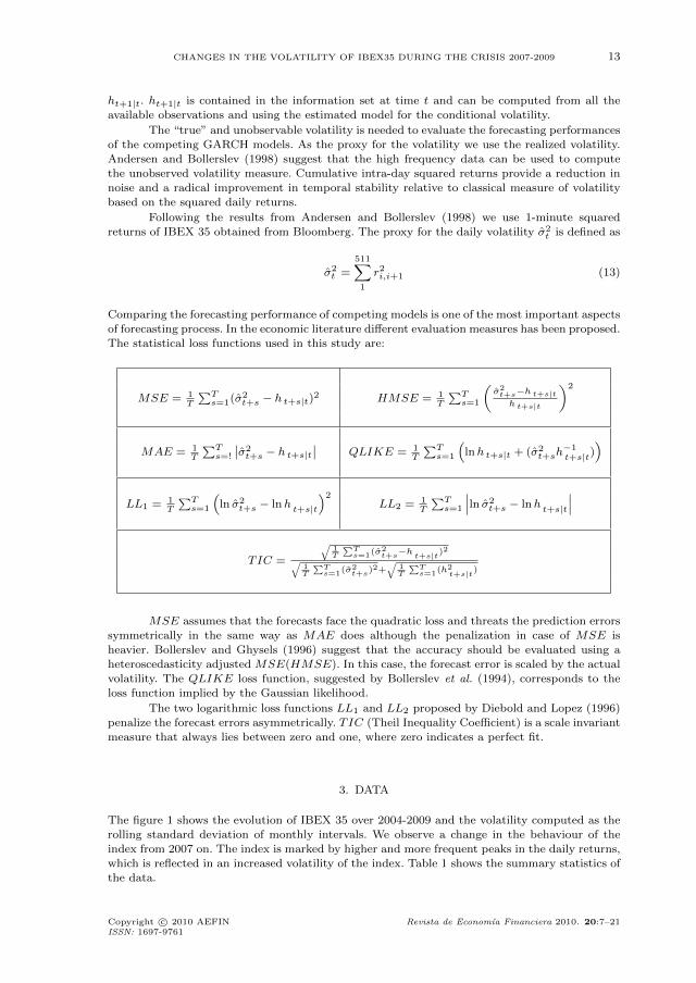
Comparing the forecasting performance of competing models is one of the most important aspectsof forecasting process. In the economic literature different evaluation measures has been proposed.

The statistical loss functions used in this study are:

MSE = 1T

∑Ts=1(σ2

t+s − h t+s|t)2 HMSE = 1

T

∑Ts=1

(σ2t+s−h t+s|th t+s|t

)2

MAE = 1T

∑Ts=!

∣∣σ2t+s − h t+s|t

∣∣ QLIKE = 1T

∑Ts=1

(lnh t+s|t + (σ2

t+sh−1t+s|t)

)

LL1 = 1T

∑Ts=1

(ln σ2

t+s − lnht+s|t

)2LL2 = 1

T

∑Ts=1

∣∣∣ln σ2t+s − lnh

t+s|t

∣∣∣

TIC =

√1T

∑Ts=1(σ2

t+s−h t+s|t)2√1T

∑Ts=1(σ2

t+s)2+√

1T

∑Ts=1(h2

t+s|t)

MSE assumes that the forecasts face the quadratic loss and threats the prediction errorssymmetrically in the same way as MAE does although the penalization in case of MSE isheavier. Bollerslev and Ghysels (1996) suggest that the accuracy should be evaluated using a

heteroscedasticity adjusted MSE(HMSE). In this case, the forecast error is scaled by the actualvolatility. The QLIKE loss function, suggested by Bollerslev et al. (1994), corresponds to theloss function implied by the Gaussian likelihood.

The two logarithmic loss functions LL1 and LL2 proposed by Diebold and Lopez (1996)penalize the forecast errors asymmetrically. TIC (Theil Inequality Coefficient) is a scale invariantmeasure that always lies between zero and one, where zero indicates a perfect fit.

3. DATA

The figure 1 shows the evolution of IBEX 35 over 2004-2009 and the volatility computed as therolling standard deviation of monthly intervals. We observe a change in the behaviour of theindex from 2007 on. The index is marked by higher and more frequent peaks in the daily returns,

which is reflected in an increased volatility of the index. Table 1 shows the summary statistics ofthe data.


14 BRYCHCY

-10

0

10

IBEX 2004-2009 and Rolling Standard Deviation (Window Width 1 month)

06/04 12/04 06/05 12/05 06/06 12/06 06/07 12/07 06/08 12/080

2

4

6

Figure 1. IBEX 35 returns (upper plot) and the rolling standard deviation (lower plot) over 2004-2009.

IBEX 35Mean St.Dev Max Min Skewness Kurtosis ADF test

0.0102 1.4203 10.11 -9.58 -0.11 12.55 -37.89 (0.000)

Table 1. The main statistics of the data.

The mean is very low and almost zero although the series has the maximum returnsof 10.11% and minimum of -9.58%. The skewness is negative which shows that the returns are

left-skewed and the kurtosis indicates fat tails in the distribution. The value of the AugmentedDickey Fuller Test (the critical value of -2.8619 at 5% level of significance) shows that the series

is stationary.

We apply the ARMA filter (the lowest value of the Schwarz Information Criterion we have

obtained for ARMA(1,1)) for estimation of volatility models and evaluation of the forecasts.

We apply the ARCH-LM test of Engle (1982) to the series of residuals εt obtained fromthe mean equation. For the valued of q = 1, ..., 5 we obtain following values of ARCH-LM teststatistic – ARCH(1)=37.19 and ARCH(5)=70.55 with the p − values = 0.0000 for both tests.Clearly we have the presence of ARCH effects in conditional volatility.

We can further investigate the nature of the ARCH effects by the means of the Sign Bias,

Negative Size Bias and Positive Size Bias tests proposed by Engle and Ng (1993).

For the Sign Bias we have obtained the value of the t -statistic for the parameter γ1 of

3.8203, for the Negative Size Bias of -11.33 and for the Positive Size Bias of 0.3449. There issubstantial evidence of asymmetric ARCH effects, coming especially from negative returns.

The first part of the sample 2004 - 2006 covers the period of rapid development of the stockmarket in Spain, driven by the strong economic growth, full integration in the world economy

and the expansion of the Spanish companies outside the country. On the other hand from March2007 the world, European and Spanish economy experience the most severe, initially financial,but than economic, crises from the Great Depression.

The table 2 below shows the average return and standard deviation of returns for these

periods.

The Table 2 shows how differently the index was behaving over the period of interest. The

first subsample (2004-2006) is characterized by the positive average returns and low volatility,

the second (2007-2009) has a negative average return but at the same time much higher volatility



Full Sample 2004-2006 2007-2009

Mean 0.0102 0.0781 -0.0767St.Deviation 1.4203 0.7806 1.9528

Table 2. The average returns and standard deviation of IBEX 35.

of the returns. The Figure 2 shows the daily changes in the index over this period of crisis.

IV V VI VII VIII IX X XI XII.07 I II III IV V VI VII VIII IX X XI XII.08 I II III IV

-10

-8

-6

-4

-2

0

2

4

6

8

10

12IBEX March 2007 - April 2009

Figure 2. IBEX 35 returns March 2007 – April 2009.

The financial and economic crisis 2007-2009 that started with credit crunch in March2007 brought a lot of volatility to the stock markets across the world and daily movements of

the indexes and individual stocks not noticed before.Over this period IBEX 35 moved seven times above 5% daily return and eight time below

the negative 5% return. On 10/10/2008 the index fell by 9.14%, the biggest drop in its history.

It was a final chapter of the turbulent week that suffered the decline of 21% of the value ofthe index. Panic seemed spread to other than financial sectors with heavy punishment of leadingenergy suppliers and telecoms. On this single day Banco Santander lost 11.95%, Telefonica 9.10%,

BBVA 11.37%, Iberdrola 10.57%.Three day later, on 13/10/2008, the index rose by 10.65%, its biggest daily increase since

its creation. The markets worldwide surged in value following the efforts of the governments

to ease the effects of the financial crises. Over the weekend the G-7 governments agreed on ajoint plan to face the crises, consisting in supporting financial institutions and guaranteeing theinterbank loans. The main gainers of the day were the big blue chips of the market - Banco

Santander rose by 12.35%, Telefonica 9.57%, BBVA 10.16%, Iberdrola 18.80%.These dramatic changes of the index motivate the investigation of the correct model for

volatility of the index.

4. EMPIRICAL RESULTS

In this section we present and discuss the results of empirical estimation of the models. First we

discuss the results of the structural test in volatility equation, estimation of the volatility models


16 BRYCHCY

and present the results of volatility forecasting.

4.1. Structural tests in volatility

As mentioned before Andrews (1993) and Andrews and Ploberger (1994) develop tests for

structural breaks which are valid for unknown break points and provide asymptotic critical valuesfor these test statistics. Hansen (1997) presents numerical procedures for computing approximate

asymptotic p− values for these statistics.

We allow for structural breaks in all the parameters of the unconditional volatilityequation at unknown break point. To capture the asymmetric behavior of volatility we use the

QGARCH(1, 1) model proposed by Sentana (1995). We allow for a potential structural break

at the end of every month (at time τ) between 15% and 85% of the sample. For each potentialbreak point τ we estimate the conditional volatility specification given as

σ2t = I[τ ](ω1 + γ1εt−1 + α1ε

2t−1 + β1σ

2t−1) + (1 − I[τ ])(ω2 + γ2εt−1 + α2ε

2t−1 + β2σ

2t−1) (14)

For each potential point of break at time τ we define the test statistic as Fn(τ) = −2(lr − lu),where lr and lu are maximized valued of the loglikelihood function of the restricted and

unrestricted model, respectively.

The Figure 3 shows the values of Fn(τ) for each month from October 2004 to June 2008.

12.2004 06.2005 12.2005 06.2006 12.2006 06.2007 12.2007 06.20085

10

15

20

25

30

35

40

45

50Structural Break Test Statistics

Figure 3. Structural Break test statistics.

The Table 3 shows the supLM, aveLM and expLM structural break test statistics of

Andrews (1993) and Andrews and Ploberger (1994) with numerical p-values calculated as inHansen (1997).

supFn ExpFn AveFn

Stat 42.23 20.35 28.55p-value 0.0000 0.0000 0.0000

Table 3. Structural break tests.



We observe a break in conditional volatility of oil prices around June 2007, few monthsafter the financial crisis has started (where the test statistic takes the highest value). We also

checked the presence of the structural break using other asymmetric GARCH model. We applythe model proposed by Glosten, Jagannathan and Runkle (1993) (GJR-GARCH), which allows

for asymmetric effects of positive and negative shocks on volatility and the Volatility Switching

GARCH model of Fornari and Mele (1996), further extension of the GJR-GARCH model thatalso takes into account the diference between the forecasted and realized volatility, and detect

the structural break in June 2007 as well.

Table 4 and Table 5 show the estimated GARCH model for IBEX returns on the date of

the break (June 2007) and for the full sample.

IBEX

ω1 α1 γ1 β1 ω2 α2 γ2 β2

0.1257∗ 0.0934∗ −0.2072∗ 0.7331∗ 0.0703∗ 0.0695∗ −0.2461∗ 0.9067∗

(0.0314) (0.0351) (0.0426) (0.0620) (0.0260) (0.0191) (0.0514) (0.0202)

Q(5) Q(10) Q(5)2 Q(10)2

3.0092 3.7893 2.8709 4.8679(0.6985) (0.9563) (0.7198) (0.8998)

Table 4. The results of the estimation of the conditional variance equation, in parenthesis the standarderror, * significant at 5% level of significance, Q(5) and Q(10) are the values of the Ljung-Box teststatistic for the presence of correlation at lag 5 and 10 in the series of standardized and squared

standardized residuals.

IBEXω α γ β Q(5) Q(10) Q(5)2 Q(10)2

0.0528∗ 0.0971∗ −0.1693∗ 0.8668∗ 2.0372 3.0001 6.1129 9.4589(0.0146) (0.0181) (0.0362) (0.0229) (0.8439) (0.9814) (0.2953) (0.4891)

Table 5. The results of the estimation of the conditional variance equation, in parenthesis the standarderror, * significant at 5% level of significance, Q(5) and Q(10) are the values of the Ljung-Box teststatistic for the presence of correlation at lag 5 and 10 in the series of standardized and squared

standardized residuals.

First of all the estimated models are correctly specified as Ljung-Box Q-statistics forstandardized and squared standardized residuals at lag 5 and 10 are not statistically significant.

The loglikelihood for the model with break improved comparing to the model for the fullsample (-1910.92 versus -1934.54). Schwarz Information Criterion for the model with break issmaller (2.9145 versus 2.9258) even with four additional parameters estimated.

The estimated unconditional volatility for the model for the full sample is 1.4586, whereasfor the model before break 0.7252 and after break 2.9647. This goes in line with the observedchanged in standard deviation for the pre- and post-break sample (see Table 2).

All the parameters for the models are statistically significant at 5% level of significance.

The persistence in volatility, the clustering effect, defines the speed at which the newshocks die out. Higher persistence, defined for QGARCH model as α+β, means that the volatility

shocks die out slowly and would swing prices more than in the past. For the model with the breakwe observe the change in the persistence of volatility from 0.8266 to 0.9762. The persistence forthe post-break sample (the period of financial crises) is higher from the persistence observed inthe model for the full sample (0.9639). It shows a stronger clustering behaviour of the conditional

volatility during the period of financial meltdown.

The parameter γ that governs the impact of negative shocks on conditional volatility isas expected negative and higher in the post-break period than in the model for the full sample

and the pre-break sample. It clearly shows a stronger reaction of conditional volatility to negativeshocks in the period of financial crisis.


18 BRYCHCY

The before discussed kurtosis of the model is a linear function of the absolute value ofthe γ parameter. The kurtosis in the post-break sample is higher than in the pre-break sample

and the full sample (5.43 versus 3.76 and 5.22). This shows that the model correctly capturesthe higher number of bigger both positive and negative returns in the course of 2007-2009.

The Figure 4 shows the fitted series of volatility for both models. We observe thatespecially in the post-break sample the model with the break estimates higher level of conditional

volatility than the model for whole sample.

Jun 2004 Dec 2004Jun 2005 Dec 2005Jun 2006 Dec 2006Jun 2007 Dec 2007Jun 2008 Dec 20080

0.5

1

1.5

2

2.5

3

3.5

4

4.5

5

5.5Conditional standard deviation for the model with whole sample and the model with estimated break

breakwhole

Figure 4. Conditional standard deviation for the model of full sample and with imposed break.

As already mentioned the news impact curves are a useful tool to show how new

information is incorporated into volatility. We have computed the NIC for the model estimated

for the full sample and for the model for each of the subsamples - the pre- and post-break sampleand present them in Figure 5.

The impact of news on the conditional volatility in the pre-break sample is much smallerfor both smaller and bigger news. This is mainly due to lower unconditional variance in the period

2004-2007. On the other hand we observe first much stronger reaction of conditional volatility tonews in the period 2007-2009 (the up-shift of the curve). Also the reaction to big negative newsis much stronger in this period than in the pre-break period.

5. FORECASTING AND FORECAST EVALUATION

We have computed the out-of-sample volatility forecasts for one day, one week and one month.

To evaluate the forecast we use the 1-minute ticks for the IBEX 35 for May 2009, which we have

not used in estimation of the models.

To evaluate the out-of-sample forecasting performance of the models we use (as explained

in the section 2.4) the loss functions like MSE, HMSE, MAE, QLIKE, LL1, LL2 and TICwhich in different ways penalize the prediction errors.

The tables 6 and 7 summarize the results of volatility forecasting. Table 6 presents the

results for each loss function and Table 7 shows which model (either Full for full sample or Breakfor the model with imposed structural break in June 2007) has a lowest value of the loss function.



-10 -8 -6 -4 -2 0 2 4 6 8 100

2

4

6

8

10

12

14

16

18News Impact Curve - QGARCH

full samplepre-breakpost-break

Figure 5. News Impact Curves for the full simple, pre- and postbreak model.

Criterion MSE HMSE MAE QLIKE LL1 LL2 TIC

1-dayFull 1.5009 0.2344 1.2251 1.4442 0.4382 0.6620 0.4303Break 1.3150 0.2187 1.1467 1.4292 0.3975 0.6305 0.4128

1-weekFull 0.6589 0.1049 0.6244 1.6849 0.1950 0.3284 0.2287Break 0.6061 0.1002 0.5787 1.6803 0.1835 0.3098 0.2161

1-monthFull 0.5681 0.1093 0.6168 1.8414 0.1173 0.2786 0.2287Break 0.5779 0.0894 0.6132 1.8419 0.1296 0.2769 0.2161

Table 6. Evaluation of the forecasting performance of the full sample and the model with the detectedbreak

Criterion MSE HMSE MAE QLIKE LL1 LL2 TIC

1-day Break Break Break Break Break Break Break1-week Break Break Break Break Break Break Break1-month Full Break Break Full Full Break Break

Table 7. Evaluation of the forecasting performance of the full sample and the model with the detectedbreak

The results of the out-of-sample forecasting show that the model with break in June 2007

is preferred for each of the forecasting period. For one-day and one-week forecasting horizon themodel with break produces better forecasts as indicated by all the loss functions. For the one-

month forecasting period the model with break is preferred by the majority of the evaluation

indicators.

Assuming that the economic stability will finally be restored in the markets the volatilityof the .nancial variable should return to the normal levels. It will be interesting to redo the

exercise to detect another break after which the model inducing lower volatility should be used

for forecasting purposes.


20 BRYCHCY

6. CONCLUSIONS

This paper investigates the structural break in the volatility of IBEX 35. We investigate the

volatility of the index over the period 2004-2009, the period that encompasses the period of

strong increases in the index and the period of the one of the most severe crises.Applying the Quadratic GARCH model and the LLM-test for possible break in the

conditional volatility at the end of every month, we detect a structural break test around

June 2007, few months after the beginning of .nancial and economic crisis. We also applyother asymmetric GARCH models to check the robustness of our findings. We observe different

behaviour of conditional volatility in the pre- and post-break sample. The post break sample is

determined by the higher unconditional volatility and stronger reaction to negative shocks. Wecheck the forecasting power of the models for full sample and the model with the detected break

in June 2007. The post-break model shows a better forecasting performance than the full samplemodel.

REFERENCES

Aggarwal, R., C. Inclan and R.Leal, 1999. Volatility in Emerging Stock Markets, Journal of Financial andQuantitative Analysis 34, 33-55.

Andersen, T.G., T. Bollerslev, 1998. Answering the Skeptics: Yes, Standard Volatility Models Do ProvideAccurate Forecasts, International Economic Review 39, 885-905.

Andrews, D.W.K., 1993. Tests for Parameter Instability and Structural Change with Unknown Change Point,Econometrica 61, 821-856.

Andrews, D.W.K., W. Ploberger, 1994. Optimal Tests when a Nuisance Parameter is Present Only Under theAlternative, Econometrica 62, 1383-1414.

Becketti, S., G.Sellon, 1989. Has Financial market volatility increased?, Federal Reserve Bank of Kansas City,Economic Review 2, 17-30.

Black, F., 1976. Studies on stock price volatility changes, Proceedings of the American Statistical Association,Business and Economic Statistics Section, 177-81.

Blanchard, O., 2009. (Nearly) nothing to fear but fear itself, The Economist, January 31st 2009.

Bollerslev, T., 1986. Generalized autoregressive heteroscedasticity, Journal of Econometrics 31, 307-327.

Bollerslev, T., E. Ghysels, 1996. Periodic autoregressive conditional heteroscedasticity, Journal of Business andEconomic Statistics, 14, 139-157.

Bollerslev, T., J. Wooldridge, 1992. Quasi-Maximum Likelihood Estimation and Inference in Dynamic Modelswith Time Varying Covariance, Econometric Reviews 11, 143-172.

Capiello, L., Engle, R.F. and K. Sheppard, 2006. Asymmetric Dynamics in the Correlations of Global Equityand Bond Returns, Journal of Financial Econometrics 4, 537-572.

Cunado, J.C., Gomez Biscarri, J. and F. Perez de Gracia Hidalgo, 2004. Structural changes in volatility andstock market development: Evidence from Spain, Journal of Banking & Finance 28, 1745-1773.

Diebold, F., J.Lopez, 1996. Forecast evaluation and combination in G. Maddala and C. Rao, Hanbook ofStatistics, Elsevier, Amsterdam.

Engle, R.F., 1982. Autoregressive conditional heteroscedasticity with estimates of the variance of UnitedKingdom inflation, Econometrica 20, 987-1007.

Engle, R.F., V.K. Ng, 1993. Measuring and Testing the Impact of News on Volatility, Journal of Finance 48,1749-1778.

Fornari, F., A. Mele, 1996. Modeling the changing asymmetry of conditional variances, Economics Letters 50,



197-203.

Franses. P. H., D. van Dijk, 1996. Forecasting stock market volatility using (nonlinear) GARCH models, Journalof Forecasting 15, 229-235.

Gil-Alana, L., Cunado, J. and F. Perez de Gracia, 2008. Stochastic volatility in the Spanish stock market: along memory model with a structural break, European Journal of Finance 14, 23-31.

Glosten, R.T., Jagannathan, R. and D. Runkle, 1993. On the Relation between the Expected Value and theVolatility of the Nominal Excess Return on Stocks, Journal of Finance 48, 1779-1801.

Hansen, B.E., 1997. Approximate Asymptotic P Values for Structural-Change Tests, Journal of Business andEconomic Statistics 15, 60-67.

Inclan, C., G.C. Tiao, 1994. Use of Cumulative Sums of Squares for Retrospective Detection of Changes ofVariance, Journal of American Statistical Association 89, 913-923.

Lamoureux, Ch.G., W.D. Lastrapes, 1990. Persistence in Variance, Structural Change and the GARCH model,Journal of Business and Economic Statistics 8, 225-234.

Pagan, A., G.W. Schwert, 1990. Alternative Models for Conditional Stock Volatility, Journal of Econometrics45, 267-290.

Sentana, E., 1995. Quadratic ARCH Models, Review of Economic Studies 62, 639-661.

Smith, D.R., 2008. Testing for Structural Breaks in GARCH Models, Applied Financial Economics 18, 845-862.


changes in the volatility of ibex35 during the crisis 2007 ... · changes in the volatility of...

Documents