chap 7 transportation problems
TRANSCRIPT

8/7/2019 CHAP 7 TRANSPORTATION PROBLEMS
http://slidepdf.com/reader/full/chap-7-transportation-problems 1/22
TRANSPORTATION PROBLEMS
Transportation problem is a case of LPP in which the objective is to transport
various amounts of a single homogeneous commodity to various destinations
for a minimum transport cost.
1. Feasible Solution
For a set of non negative values xij that satisfies the constraints are called the
feasible solution of the transportation problem.
2. Basic Feasible Solution
A feasible solution that contains not more than m+n-1 non negative allocation
is called BF solution to the TP.
3. Optimal Solution A feasible solution is said to be optimal if it minimizes the total transportation
cost.
4. Degenerate & Non- degenerate Basic Feasible Solution
A BF solution to the m × n TP that contains exactly m+n-1 allocation in
independent position is called non degenerate BF solution.
A feasible solution that contains less than m+n-1 non negative allocation is
said to be degenerating.
Methods to find initial basic feasible solution
1. North West Corner Rule (NWCR)
Ques : Find the IBFS whose cost matrix is given by
D1 D2 D3 D4 Capacity
6 4 1 5 14
8 9 2 7 16
4 3 6 2 15
6 10 15 14 Demand
8/7/2019 CHAP 7 TRANSPORTATION PROBLEMS
http://slidepdf.com/reader/full/chap-7-transportation-problems 2/22
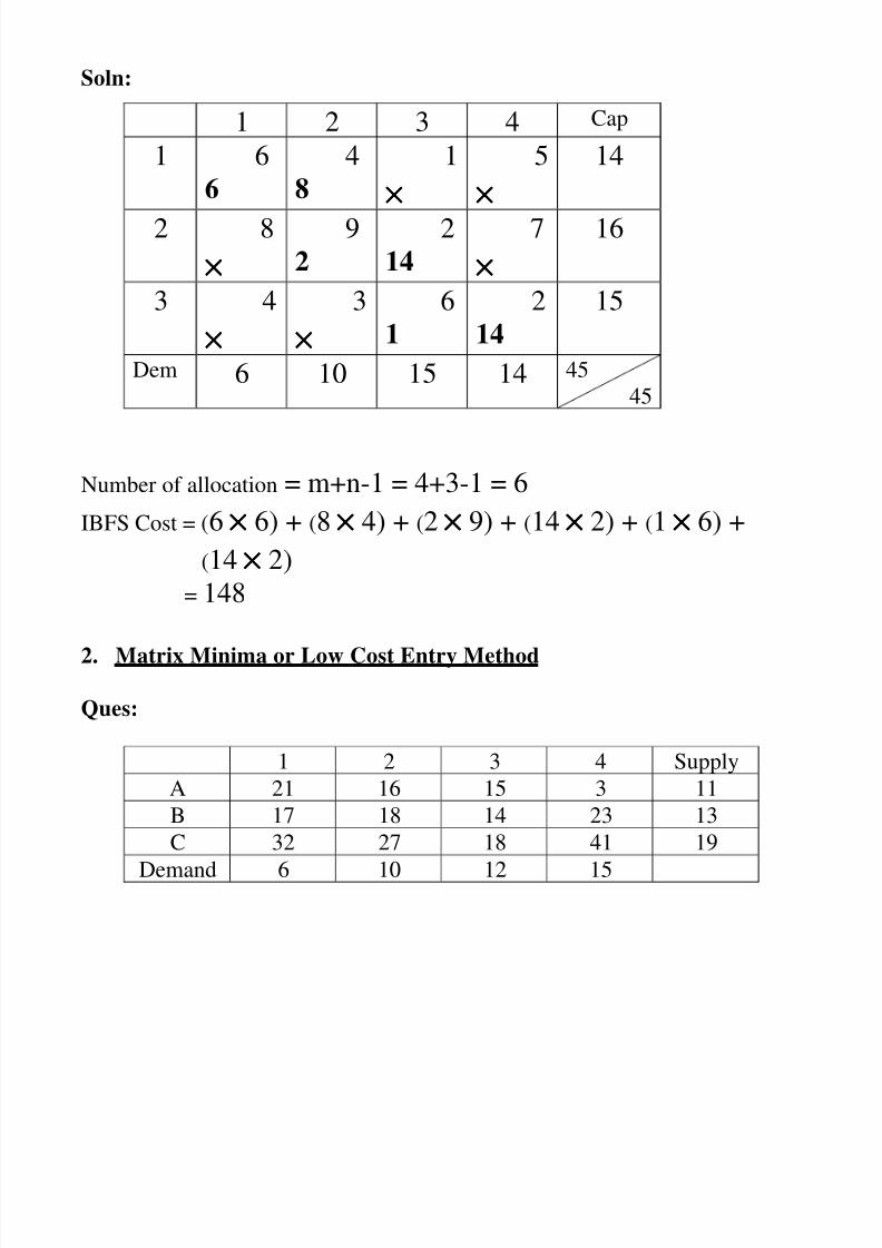
Soln:
Number of allocation = m+n-1 = 4+3-1 = 6
IBFS Cost = (6 ×××× 6) + (8 ×××× 4) + (2 ×××× 9) + (14 ×××× 2) + (1 ×××× 6) +
(14 ×××× 2)
= 148
2. Matrix Minima or Low Cost Entry Method
Ques:
1 2 3 4 Supply
A 21 16 15 3 11
B 17 18 14 23 13
C 32 27 18 41 19
Demand 6 10 12 15
1 2 3 4 Cap
1 6
6
4
8
1
×××× 5
××××
14
2 8
××××
92
214
7
××××
16
3 4
××××
3
××××
6
1
2
14
15
Dem 6 10 15 14 45
45
8/7/2019 CHAP 7 TRANSPORTATION PROBLEMS
http://slidepdf.com/reader/full/chap-7-transportation-problems 3/22
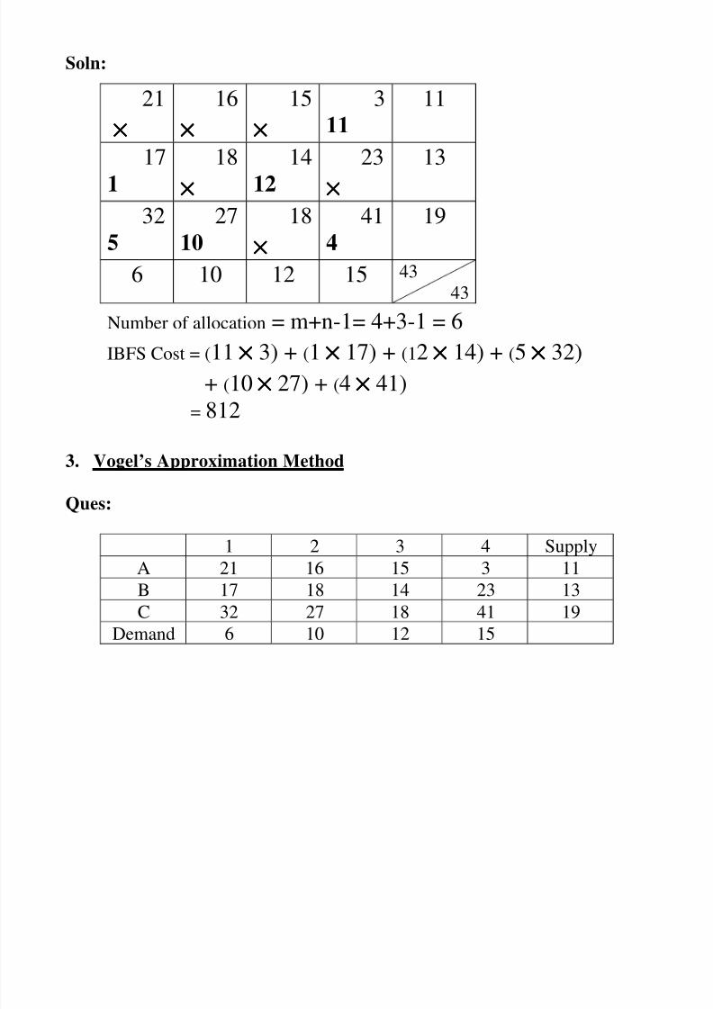
Soln:
Number of allocation = m+n-1= 4+3-1 = 6
IBFS Cost = (11 ×××× 3) + (1 ×××× 17) + (12 ×××× 14) + (5 ×××× 32)+ (10 ×××× 27) + (4 ×××× 41)
= 812
3. Vogel’s Approximation Method
Ques:
1 2 3 4 Supply
A 21 16 15 3 11
B 17 18 14 23 13
C 32 27 18 41 19
Demand 6 10 12 15
21
××××
16
××××
15
×××× 3
11
11
17
1
18
××××
14
12
23
××××
13
32
5
27
10
18
××××
41
4
19
6 10 12 15 43
43
8/7/2019 CHAP 7 TRANSPORTATION PROBLEMS
http://slidepdf.com/reader/full/chap-7-transportation-problems 4/22
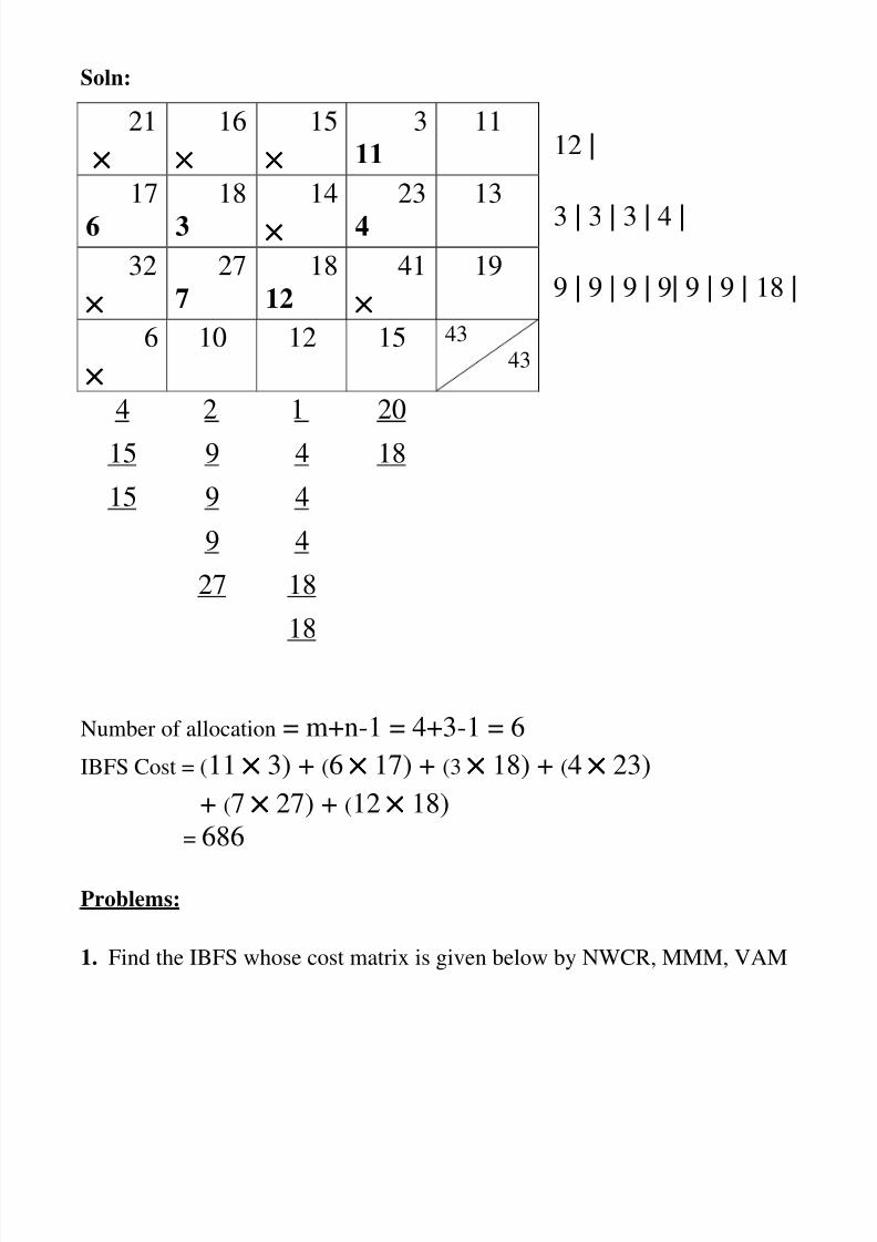
Soln:
12 |
3 | 3 | 3 | 4 |
9 | 9 | 9 | 9| 9 | 9 | 18 |
Number of allocation = m+n-1 = 4+3-1 = 6
IBFS Cost = (11 ×××× 3) + (6 ×××× 17) + (3 ×××× 18) + (4 ×××× 23)
+ (7 ×××× 27) + (12 ×××× 18)
= 686
Problems:
1. Find the IBFS whose cost matrix is given below by NWCR, MMM, VAM
21
××××
16
××××
15
×××× 3
11
11
17
6
18
3
14
××××
23
4
13
32
××××
27
7
18
12
41
××××
19
6
××××
10 12 15 43
43
4 2 1 20
15 9 4 18
15 9 4
9 4
27 18
18

8/7/2019 CHAP 7 TRANSPORTATION PROBLEMS
http://slidepdf.com/reader/full/chap-7-transportation-problems 5/22
E F G H I J Supply
A 14 19 32 9 21 0 200
B 15 10 18 7 11 0 225
C 20 12 13 18 16 0 175
D 11 32 14 14 18 0 350
Demand 130 110 140 260 180 130
Soln:
a. NWCR:
IBFS Cost = (130 ×××× 14) + (70 ×××× 19) + (40 ×××× 10) + (140 ×××× 18)
+ (45 ×××× 7) + (175 ×××× 18) + (40 ×××× 14) + (180 ×××× 18)
+ (0 ×××× 130)
= 13335
14
130
19
70
32
××××9
××××
21
××××
0
××××200
15
××××
10
40
18
140
7
45
11
××××
0
××××
225
20
×××× 12
××××
13
××××
18
175
16
××××
0
××××
175
11
××××32
××××
14
××××
14
40
18
180
0
130
350
130 110 140 260 180 130

8/7/2019 CHAP 7 TRANSPORTATION PROBLEMS
http://slidepdf.com/reader/full/chap-7-transportation-problems 6/22
b. VAM:
IBFS Cost = 10315
14
××××
19
××××
32
×××× 9
35
21
35
0
130 200 9 5 5
15××××
10××××
18××××
7225
11××××
0××××
225 7 3 3 3
20
×××× 12
110
13
65
18
××××
16
××××
0
××××
175 12 1 1 1 1
11
130 32
××××
14
75
14
××××
18
145
0
××××
350 11 3 3 3 3 3
130 110 140 260 180 130 950
3 2 1 2 5 0
3 2 1 2 5 0
3 2 1 2
4 2 1 7
9 20 1 4
11 32 14 14
8/7/2019 CHAP 7 TRANSPORTATION PROBLEMS
http://slidepdf.com/reader/full/chap-7-transportation-problems 7/22
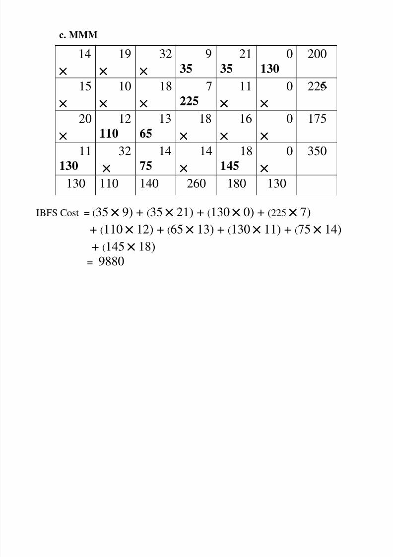
c. MMM
c.
IBFS Cost = (35 ×××× 9) + (35 ×××× 21) + (130 ×××× 0) + (225 ×××× 7)
+ (110 ×××× 12) + (65 ×××× 13) + (130 ×××× 11) + (75 ×××× 14)
+ (145 ×××× 18)
= 9880
14
××××
19
××××
32
×××× 9
35
21
35
0
130 200
15
××××
10
××××
18
××××
7
225
11
××××
0
××××
225
20
×××× 12
110
13
65
18
××××
16
××××
0
××××
175
11
130 32
××××
14
75
14
××××
18
145
0
××××
350
130 110 140 260 180 130

8/7/2019 CHAP 7 TRANSPORTATION PROBLEMS
http://slidepdf.com/reader/full/chap-7-transportation-problems 8/22
Test for optimality
1. Number of allocation = m+n-1
2. These allocations must be in independent positions
Non independent
Non independent
Independent
Prob: Test the optimality of the given problem by Modi method or UVmethod
19 30 50 10 7
70 30 40 60 9
40 8 70 20 18
5 8 7 14
8/7/2019 CHAP 7 TRANSPORTATION PROBLEMS
http://slidepdf.com/reader/full/chap-7-transportation-problems 9/22
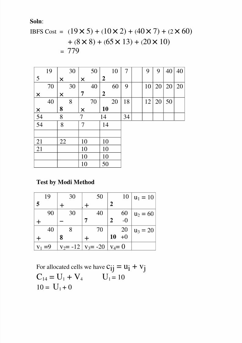
Soln:
IBFS Cost = (19 ×××× 5) + (10 ×××× 2) + (40 ×××× 7) + (2 ×××× 60)
+ (8 ×××× 8) + (65 ×××× 13) + (20 ×××× 10)
= 779
Test by Modi Method
19
5
30
+50
+
10
2u1 = 10
90
+
30
−−−−
40
7
60
2 -0u2 = 60
40
+
8
8888
70
+
20
10 +0u3 = 20
v1 =9 v2= -12 v3= -20 v4= 0
For allocated cells we have cij = ui + v j
C14 = U1 + V4 U1 = 10 10 = U1 + 0
19
5
30
××××
50
×××× 10
2
7 9 9 40 40
70
××××
30
××××
40
7
60
2
9 10 20 20 20
40
×××× 8
8
70
××××
20
10
18 12 20 50
54 8 7 14 3454 8 7 14
21 22 10 10
21 10 10
10 10
10 50

8/7/2019 CHAP 7 TRANSPORTATION PROBLEMS
http://slidepdf.com/reader/full/chap-7-transportation-problems 10/22
C24 = U2 + V4 U2 = 10 60 = U2 + 0
C34 = U3 + V4 U3 = 0 20 = U3 + 0
C11 = U1 + V1 V1 = 9 19 = V1 + 10
C23 = U2 + V3 V3 = -20
40 = V3 + 60
C32 = U3 + V2 V2 = -12 8 = V1 + 20
For empty cells
dij
= cij – ( u
j + v
j )
d12 = 30 – (10 – 12 )d12 = 32
d13 = 50 – (10 – 20 )d13 = 60
d21 = 90 – (9 + 60 ) d22 = 30 – (60 – 12 )d21 = 21 d22 = -18
d31 = 40 – (9 + 20 ) d33 = 70 – (20 – 20 )d31 = 11 d33 = 70 Ans: 743
8/7/2019 CHAP 7 TRANSPORTATION PROBLEMS
http://slidepdf.com/reader/full/chap-7-transportation-problems 11/22
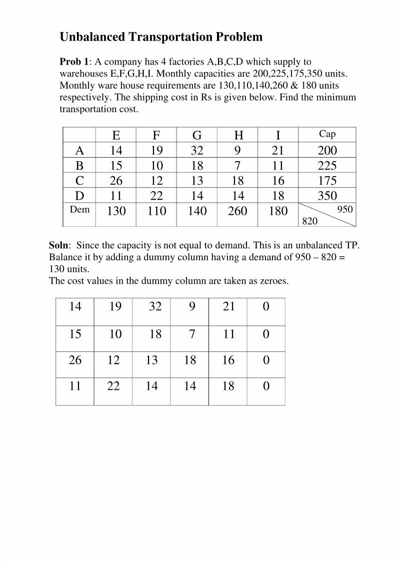
Unbalanced Transportation Problem
Prob 1: A company has 4 factories A,B,C,D which supply to
warehouses E,F,G,H,I. Monthly capacities are 200,225,175,350 units.
Monthly ware house requirements are 130,110,140,260 & 180 units
respectively. The shipping cost in Rs is given below. Find the minimumtransportation cost.
Soln: Since the capacity is not equal to demand. This is an unbalanced TP.
Balance it by adding a dummy column having a demand of 950 – 820 =
130 units.
The cost values in the dummy column are taken as zeroes.
14 19 32 9 21 0
15 10 18 7 11 0
26 12 13 18 16 0
11 22 14 14 18 0
E F G H I Cap
A 14 19 32 9 21 200
B 15 10 18 7 11 225
C 26 12 13 18 16 175
D 11 22 14 14 18 350Dem 130 110 140 260 180 950
820

8/7/2019 CHAP 7 TRANSPORTATION PROBLEMS
http://slidepdf.com/reader/full/chap-7-transportation-problems 12/22
14
××××
19
××××
32
×××× 9
200
21
××××
0
×××× 200
15
××××
10
××××
18
××××
7
45
11
80
0
××××
225
26
×××× 12
45
13
××××
18
××××
16
××××
0
130
175
11
130 22
65
14
140
14
15
18
××××
0
××××
350
130 110 140 260 180 130
14
××××
19
××××
32
×××× 9
200
21
××××
0
×××× 200
15
××××
10
××××
18
××××
7
45
11
80
0
××××
225
26
×××× 12
45
13
××××
18
××××
16
××××
0
130
175
11
130 22
65
14
140
14
15
18
××××
0
××××
350
14
××××
19
××××
32
×××× 9
200
21
××××
0
××××15
××××
10
××××
18
××××
7
60
11
165
0
××××
26
×××× 1245
13
××××
18
××××
16
××××
0130
11
130 22
65
14
40
14
××××
18
15
0
××××

8/7/2019 CHAP 7 TRANSPORTATION PROBLEMS
http://slidepdf.com/reader/full/chap-7-transportation-problems 13/22
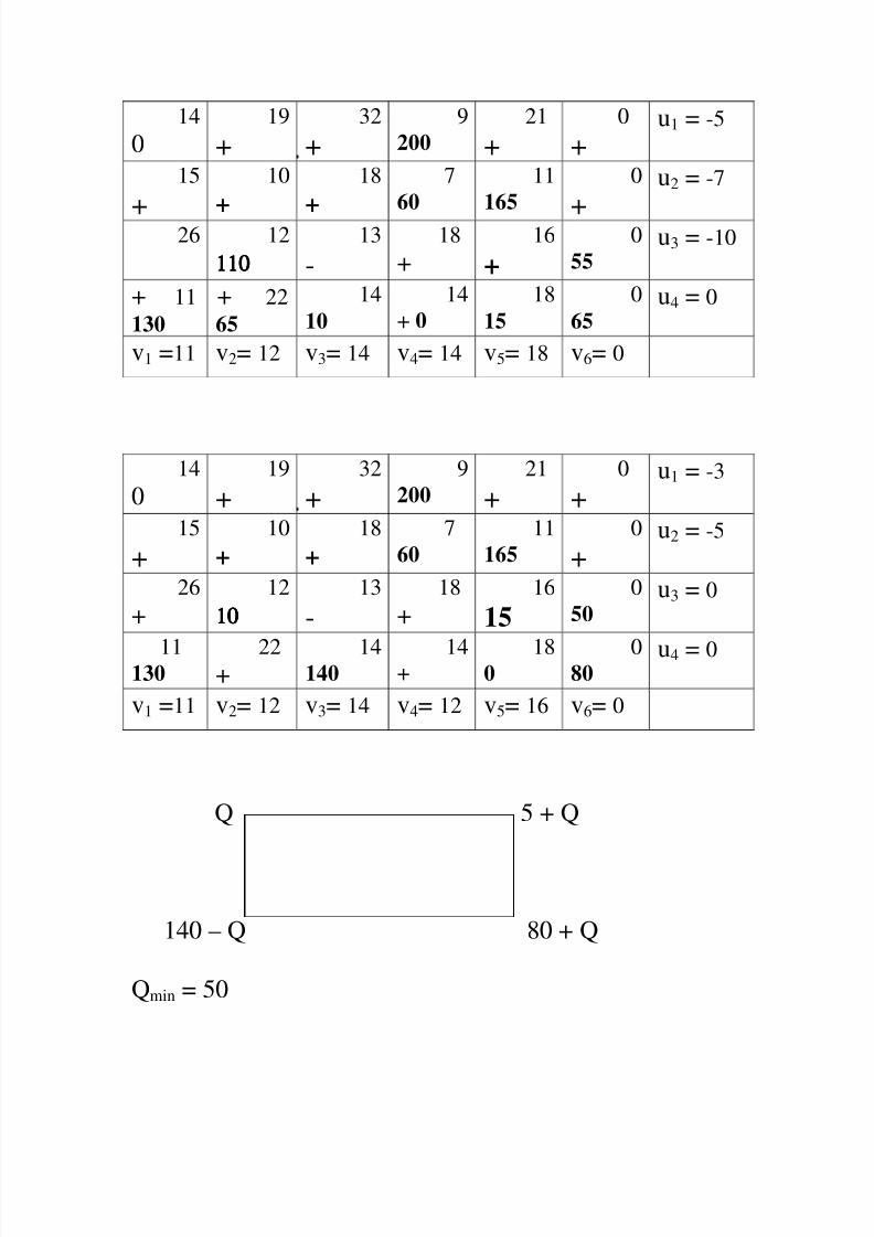
Test for optimality
14
+19
+32
+
9
200
21
+
u1 = -5
5
+
30
−−−−
40
7
60
2 -0
11
165
u2 = -7
26
+
8
8888
70
+
20
10 +0
16
+u3 = -10
11
130
22
65
14
140
14
0
18
100 u4 = 0
v1 =11 v2= 22 v3= 14 v4= 14 v5= 18 v6= 10
(45 + 0) Q -Q (130-0)
(65 – 0) –Q Q
130 – Q = 0And, 65 – 0 =0
Q = 65 & 130
Qmin = 65
Q 65 - Q
15 – Q 65 + Q
Qmin = 15
8/7/2019 CHAP 7 TRANSPORTATION PROBLEMS
http://slidepdf.com/reader/full/chap-7-transportation-problems 14/22
8/7/2019 CHAP 7 TRANSPORTATION PROBLEMS
http://slidepdf.com/reader/full/chap-7-transportation-problems 15/22
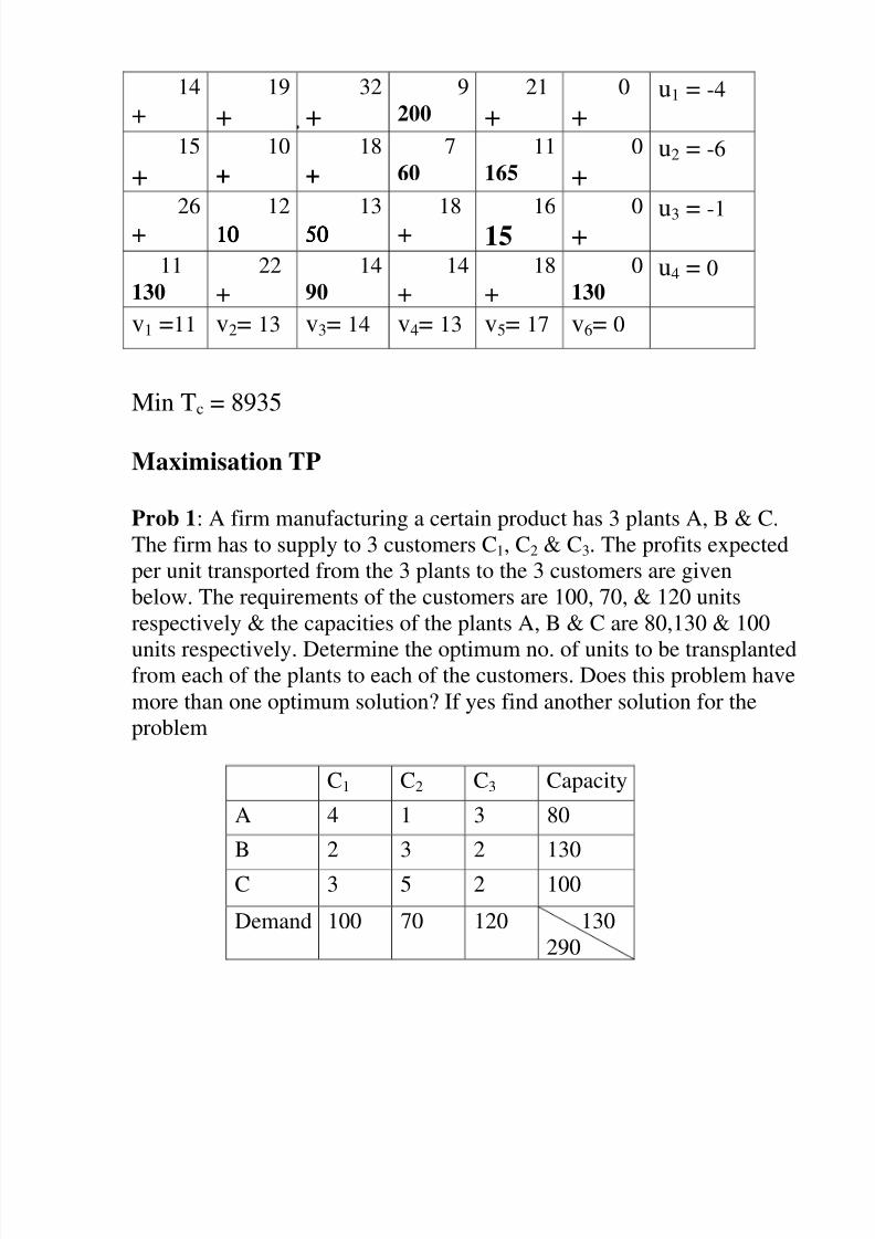
Min Tc = 8935
Maximisation TP
Prob 1: A firm manufacturing a certain product has 3 plants A, B & C.
The firm has to supply to 3 customers C1, C2 & C3. The profits expected
per unit transported from the 3 plants to the 3 customers are given
below. The requirements of the customers are 100, 70, & 120 units
respectively & the capacities of the plants A, B & C are 80,130 & 100
units respectively. Determine the optimum no. of units to be transplantedfrom each of the plants to each of the customers. Does this problem have
more than one optimum solution? If yes find another solution for the
problem
C1 C2 C3 Capacity
A 4 1 3 80
B 2 3 2 130
C 3 5 2 100
Demand 100 70 120 130
290
14
+19
+32
+
9
200
21
+
0
+
u1 = -4
15
+
10
+
18
+
7
60
11
165
0
+
u2 = -6
26+ 1210101010 1350505050 18+ 1615 0+ u3 = -1
11
130
22
+
14
90
14
+
18
+
0
130 u4 = 0
v1 =11 v2= 13 v3= 14 v4= 13 v5= 17 v6= 0

8/7/2019 CHAP 7 TRANSPORTATION PROBLEMS
http://slidepdf.com/reader/full/chap-7-transportation-problems 16/22
Soln: Since the capacity is not equal to demand. This is an unbalanced
TP. Balance it by adding a dummy column having a demand of 310 –
290 = 20 units.
C1 C2 C3 C4 Capacity
A 4 1 3 0 80
B 2 3 2 0 130
C 3 5 2 0 100
Demand 100 70 120 20
Since the given matrix is a profit matrix it has to be maximized. The
given matrix is converted to solve for maximization.
(1) Select highest element in the matrix and subtract all other
elements from it.
For the revised matrix apply regular procedure
IBFS Cost = (70 ×××× 4) + (10 ×××× 3) + (110 ×××× 2) + (20 ×××× 0)
+ (30 ×××× 3) + (70 ×××× 5)
= 970
1
70
4
××××
10
×××× 5
××××
80 1 1 1 3
3
××××
2
××××
3110
520
130 1 0 1 2
2
30 0
70
3
××××
5
××××
100 2 1
100 70 120 20
1 2 1 0
1 1 0
2 1 0
1 0
8/7/2019 CHAP 7 TRANSPORTATION PROBLEMS
http://slidepdf.com/reader/full/chap-7-transportation-problems 17/22
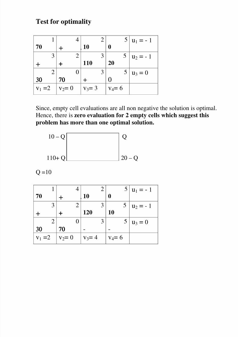
Test for optimality
Since, empty cell evaluations are all non negative the solution is optimal.
Hence, there is zero evaluation for 2 empty cells which suggest thisproblem has more than one optimal solution.
10 – Q Q
110+ Q 20 – Q
Q =10
1
70 4
+2
10
5
0u1 = - 1
3+ 2+ 3110 520 u2 = - 1
2
30303030 0
70707070
3
+
5
0u3 = 0
v1 =2 v2= 0 v3= 3 v4= 6
1
70 4
+2
10
5
0u1 = - 1
3
+
2
+
3
120
5
10u2 = - 1
2
30303030 0
70707070
3
- 5
-u3 = 0
v1 =2 v2= 0 v3= 4 v4= 6
8/7/2019 CHAP 7 TRANSPORTATION PROBLEMS
http://slidepdf.com/reader/full/chap-7-transportation-problems 18/22
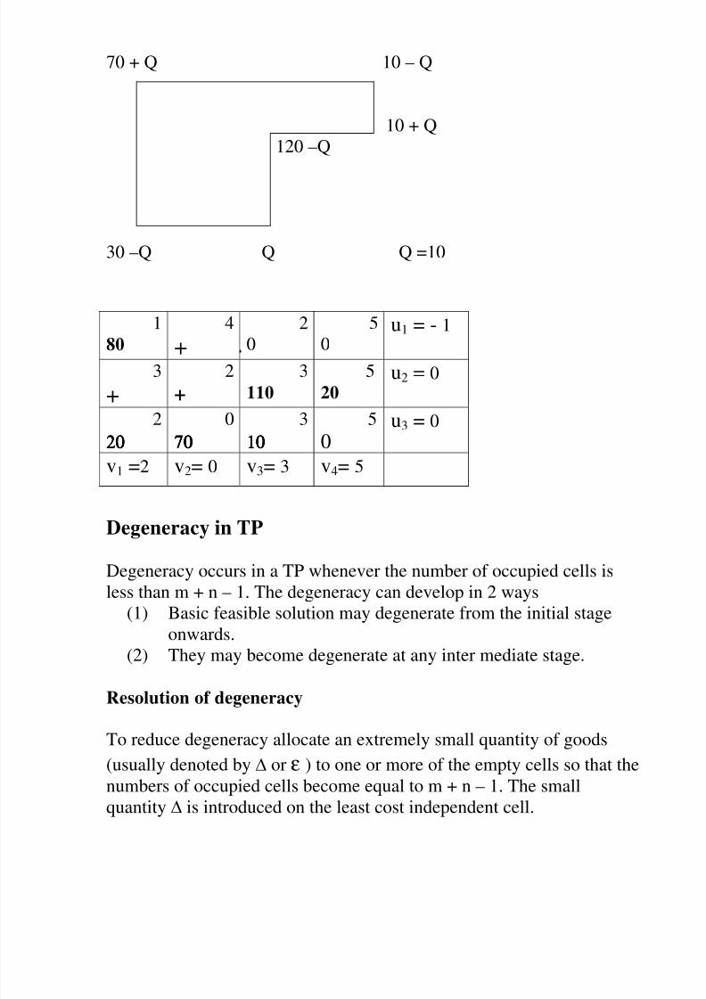
70 + Q 10 – Q
10 + Q
120 –Q
30 –Q Q Q =10
Degeneracy in TP
Degeneracy occurs in a TP whenever the number of occupied cells is
less than m + n – 1. The degeneracy can develop in 2 ways
(1) Basic feasible solution may degenerate from the initial stage
onwards.
(2) They may become degenerate at any inter mediate stage.
Resolution of degeneracy
To reduce degeneracy allocate an extremely small quantity of goods
(usually denoted by or ε ) to one or more of the empty cells so that the
numbers of occupied cells become equal to m + n – 1. The small
quantity is introduced on the least cost independent cell.
1
80
4
+
2
0
5
0
u1 = - 1
3
+
2
+
3
110
5
20u2 = 0
2
20202020 0
70707070
3
10101010
5
0u3 = 0
v1 =2 v2= 0 v3= 3 v4= 5
8/7/2019 CHAP 7 TRANSPORTATION PROBLEMS
http://slidepdf.com/reader/full/chap-7-transportation-problems 19/22
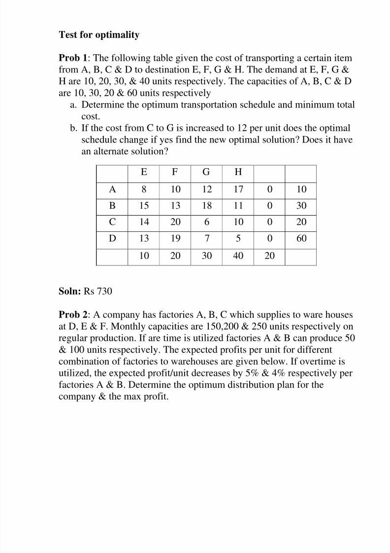
Test for optimality
Prob 1: The following table given the cost of transporting a certain item
from A, B, C & D to destination E, F, G & H. The demand at E, F, G &
H are 10, 20, 30, & 40 units respectively. The capacities of A, B, C & D
are 10, 30, 20 & 60 units respectivelya. Determine the optimum transportation schedule and minimum total
cost.
b. If the cost from C to G is increased to 12 per unit does the optimal
schedule change if yes find the new optimal solution? Does it have
an alternate solution?
Soln: Rs 730
Prob 2: A company has factories A, B, C which supplies to ware houses
at D, E & F. Monthly capacities are 150,200 & 250 units respectively on
regular production. If are time is utilized factories A & B can produce 50
& 100 units respectively. The expected profits per unit for different
combination of factories to warehouses are given below. If overtime is
utilized, the expected profit/unit decreases by 5% & 4% respectively per
factories A & B. Determine the optimum distribution plan for thecompany & the max profit.
E F G H
A 8 10 12 17 0 10B 15 13 18 11 0 30
C 14 20 6 10 0 20
D 13 19 7 5 0 60
10 20 30 40 20
8/7/2019 CHAP 7 TRANSPORTATION PROBLEMS
http://slidepdf.com/reader/full/chap-7-transportation-problems 20/22
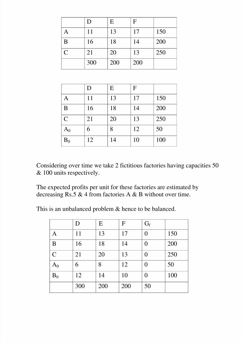
D E F
A 11 13 17 150
B 16 18 14 200
C 21 20 13 250
300 200 200
D E F
A 11 13 17 150
B 16 18 14 200
C 21 20 13 250A0 6 8 12 50
B0 12 14 10 100
Considering over time we take 2 fictitious factories having capacities 50
& 100 units respectively.
The expected profits per unit for these factories are estimated by
decreasing Rs.5 & 4 from factories A & B without over time.
This is an unbalanced problem & hence to be balanced.
D E F Gf
A 11 13 17 0 150
B 16 18 14 0 200
C 21 20 13 0 250
A0 6 8 12 0 50
B0 12 14 10 0 100
300 200 200 50
8/7/2019 CHAP 7 TRANSPORTATION PROBLEMS
http://slidepdf.com/reader/full/chap-7-transportation-problems 21/22
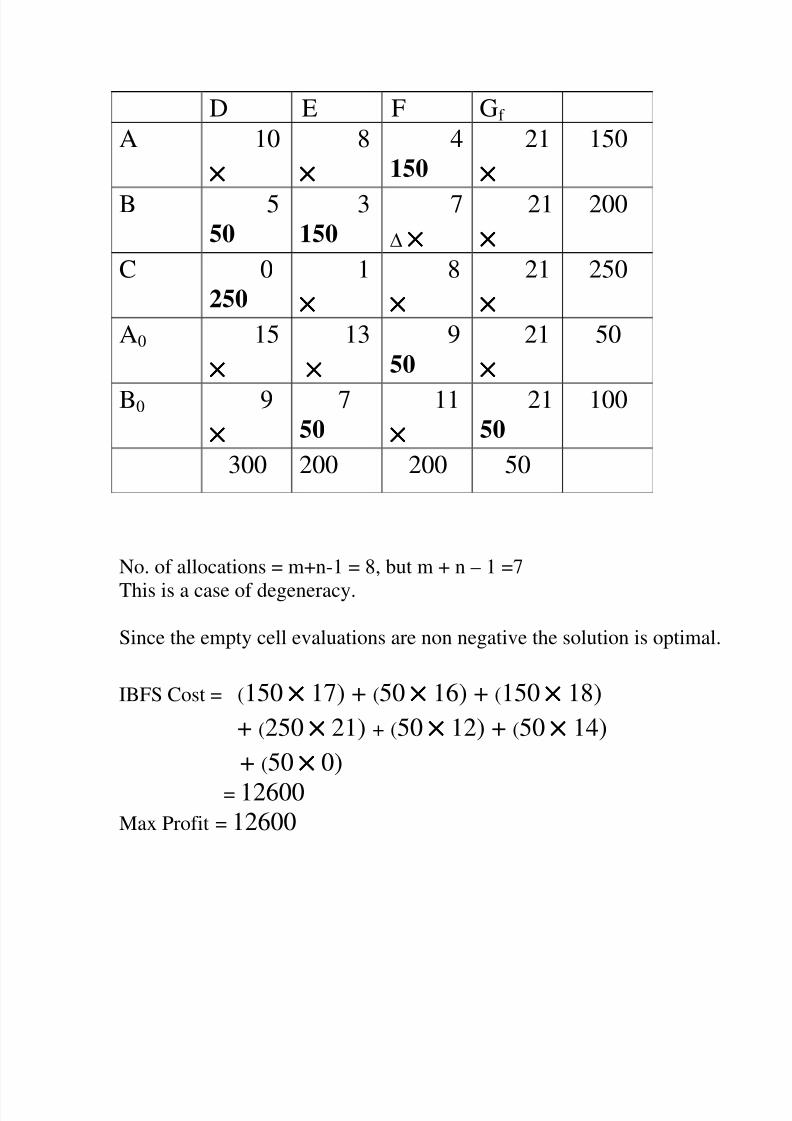
No. of allocations = m+n-1 = 8, but m + n – 1 =7
This is a case of degeneracy.
Since the empty cell evaluations are non negative the solution is optimal.
IBFS Cost = (150 ×××× 17) + (50 ×××× 16) + (150 ×××× 18)
+ (250 ×××× 21) + (50 ×××× 12) + (50 ×××× 14)
+ (50 ×××× 0)
= 12600Max Profit = 12600
D E F Gf
A 10
××××
8
××××
4
150 21
××××
150
B 550
3150
7
××××
21
××××
200
C 0
250 1
××××
8
××××
21
××××
250
A0 15
×××× 13
××××
9
50
21
××××
50
B0 9
××××
750
11
××××
2150
100
300 200 200 50

8/7/2019 CHAP 7 TRANSPORTATION PROBLEMS
http://slidepdf.com/reader/full/chap-7-transportation-problems 22/22
D E F Gf
A 10
+
8
+
4
50 21
+
u1 = -3
B 550
3150
7
21+
u2 = 0
C 0
250 1
+
8
+
21
+
u3 = -5
A0 15
+ 13
+
9
50
21
+
u4 = 2
B0
90 750 11+ 2150
u5 = 4
v1 =5 v2= 3 v3= 7 v4= 17
13
+
11
1
16
+ 23
+
u1 = -3
11
1
19
4
26
+
16
-
u2 = 8
12
+ 11
2
4
5
9
3
u3 = 0
7
8 15
0
9
+
14
+
u4 = 4
v1 = 3 v2= 11 v3= 4 v4= 9