chapter 1 – math toolbox - university of illinoislight.ece.illinois.edu/ece460/pdf/appendix 1-xx -...
TRANSCRIPT
Chapter 1 – Math Toolbox
Gabriel Popescu
University of Illinois at Urbana‐Champaign y p gBeckman Institute
Quantitative Light Imaging Laboratory
Electrical and Computer Engineering, UIUCPrinciples of Optical Imaging
Quantitative Light Imaging Laboratoryhttp://light.ece.uiuc.edu

Objectives
ECE 460 – Optical Imaging
Develop a set of tools useful throughout the course
Objectives
p g
Chapter 1: Math Toolbox 2
1.1 Linear Systems
ECE 460 – Optical Imaging
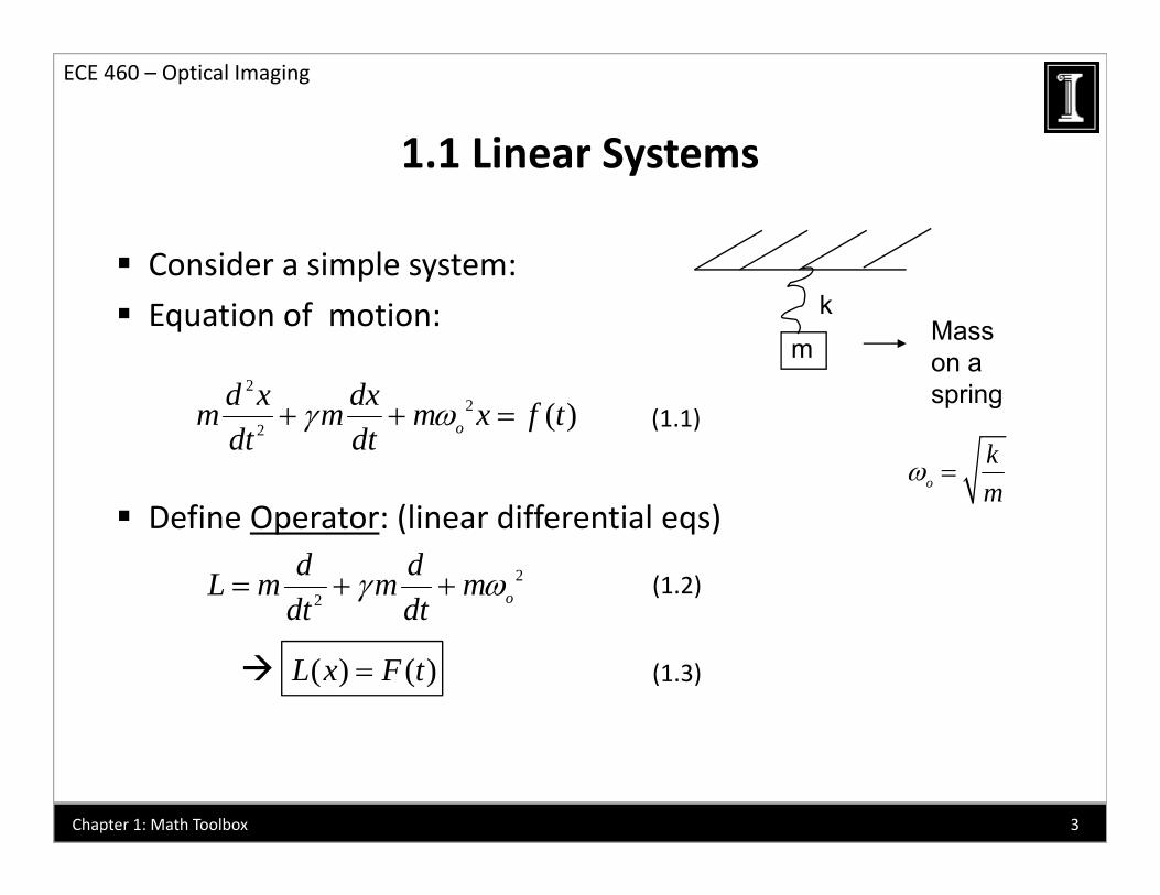
Consider a simple system:
1.1 Linear Systems
p y
Equation of motion:
2d x dxm
kMass on a spring
( )
22 ( )o
d x dxm m m x f tdt dt
o
km
(1.1)spring
Define Operator: (linear differential eqs)
22 o
d dL m m mdt dt
(1.2)
dt dt
( ) ( )L x F t (1.3)
3Chapter 1: Math Toolbox
1.1 Linear Systems
ECE 460 – Optical Imaging
Operator L has important properties:
1.1 Linear Systems
p p p p
a) 22
( ) ( )( ) ( )o
d ax d axL ax m m m axdt dt
2
dt dt2
2
( ) ( ) ( )o
d x d xa m m m xdt dt
2
b) 2( ) ( )( ) ( )d x y d x yL x y m m m x y
( )aL x (1.4)
b) ( ) ( )oL x y m m m x ydt dt
( ) ( )L x L y (1.5)
4Chapter 1: Math Toolbox
1.1 Linear Systems
ECE 460 – Optical Imaging
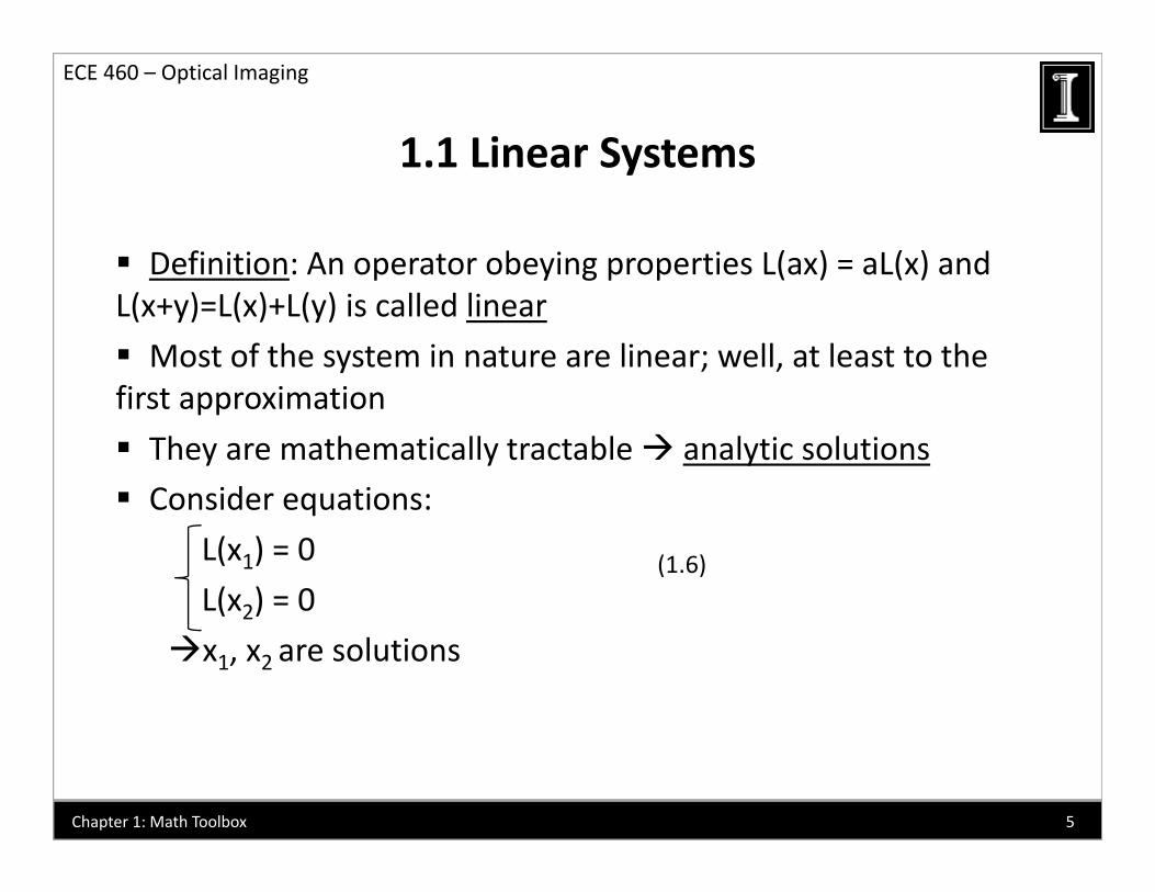
Definition: An operator obeying properties L(ax) = aL(x) and
1.1 Linear Systems
p y g p p ( ) ( )L(x+y)=L(x)+L(y) is called linear
Most of the system in nature are linear; well, at least to the fi t i tifirst approximation
They are mathematically tractable analytic solutions Consider equations:Consider equations:
L(x1) = 0
L(x2) = 0(1.6)
( 2)
x1, x2 are solutions
5Chapter 1: Math Toolbox
1.1 Linear Systems
ECE 460 – Optical Imaging
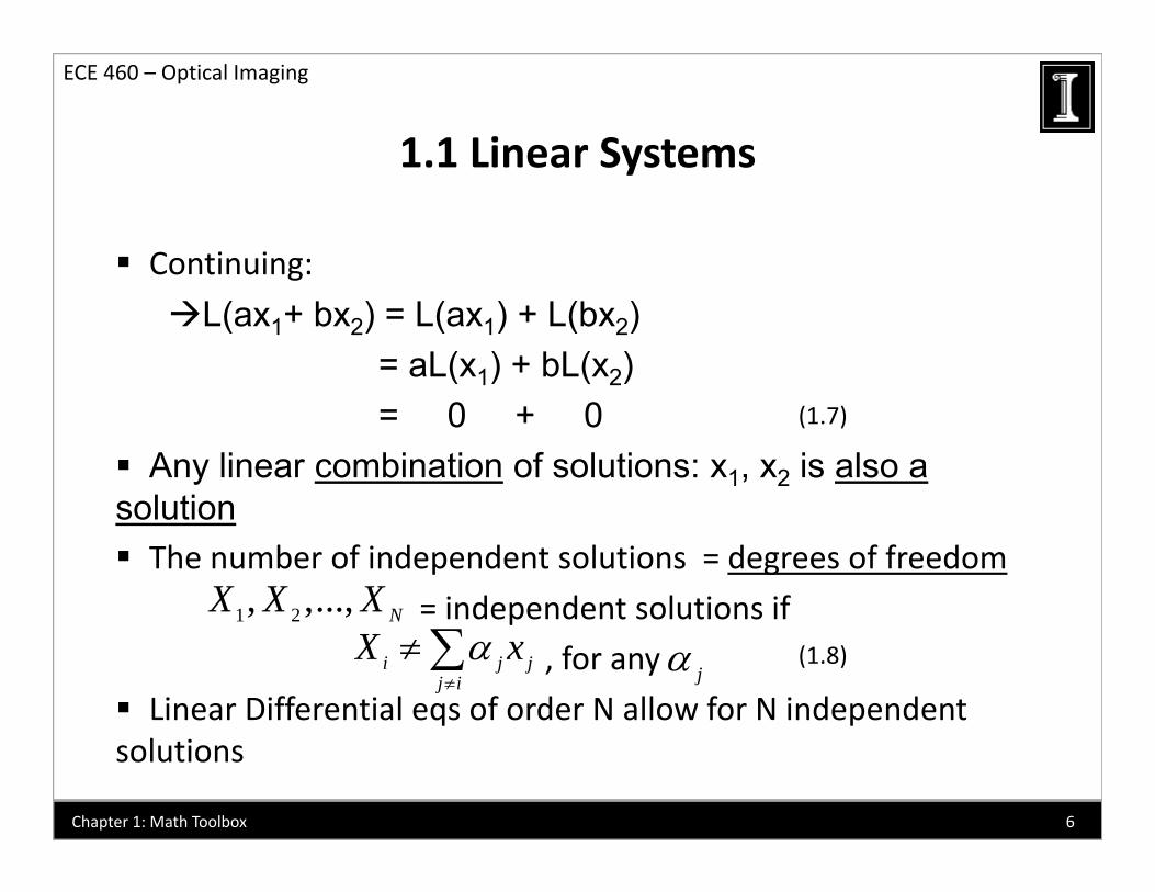
Continuing:
1.1 Linear Systems
g
L(ax1+ bx2) = L(ax1) + L(bx2)= aL(x1) + bL(x2)= 0 + 0
Any linear combination of solutions: x1, x2 is also a solution
(1.7)
solution The number of independent solutions = degrees of freedom
= independent solutions if1 2, ,..., NX X X independent solutions if
, for any
Linear Differential eqs of order N allow for N independent
1 2, , , N
i j jj i
X x
j (1.8)
solutions
6Chapter 1: Math Toolbox
1.2 Light‐matter interaction
ECE 460 – Optical Imaging
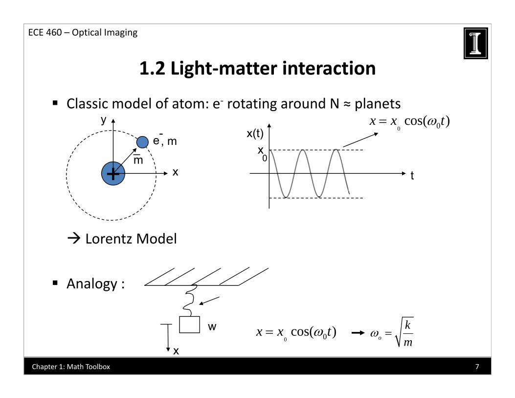
Classic model of atom: e‐ rotating around N ≈ planets
1.2 Light matter interaction
y0cos( )x x ty
+ x
e-, m
m_
x(t)
t
x0
0 0cos( )x x t
+ x t
Lorentz Model
Analogy :
kwo
km
x
w0 0cos( )x x t
7Chapter 1: Math Toolbox
1.2 Light‐matter interaction
ECE 460 – Optical Imaging
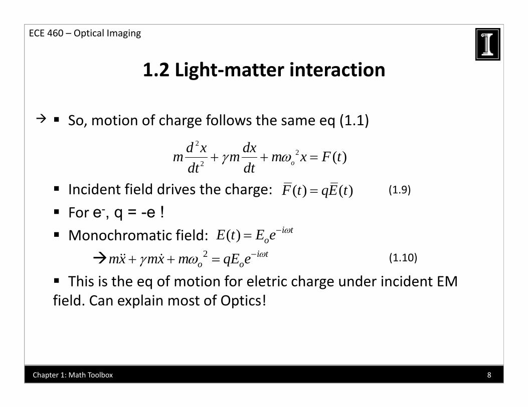
So, motion of charge follows the same eq (1.1)
1.2 Light matter interaction
, g q ( )2
22 ( )o
d x dxm m m x F tdt dt
Incident field drives the charge:
For e-, q = -e !( ) ( )F t qE t
( ) i t
(1.9)
Monochromatic field:
This is the eq of motion for eletric charge under incident EM
( ) i toE t E e
2 i to omx mx m qE e (1.10)
This is the eq of motion for eletric charge under incident EM field. Can explain most of Optics!
8Chapter 1: Math Toolbox
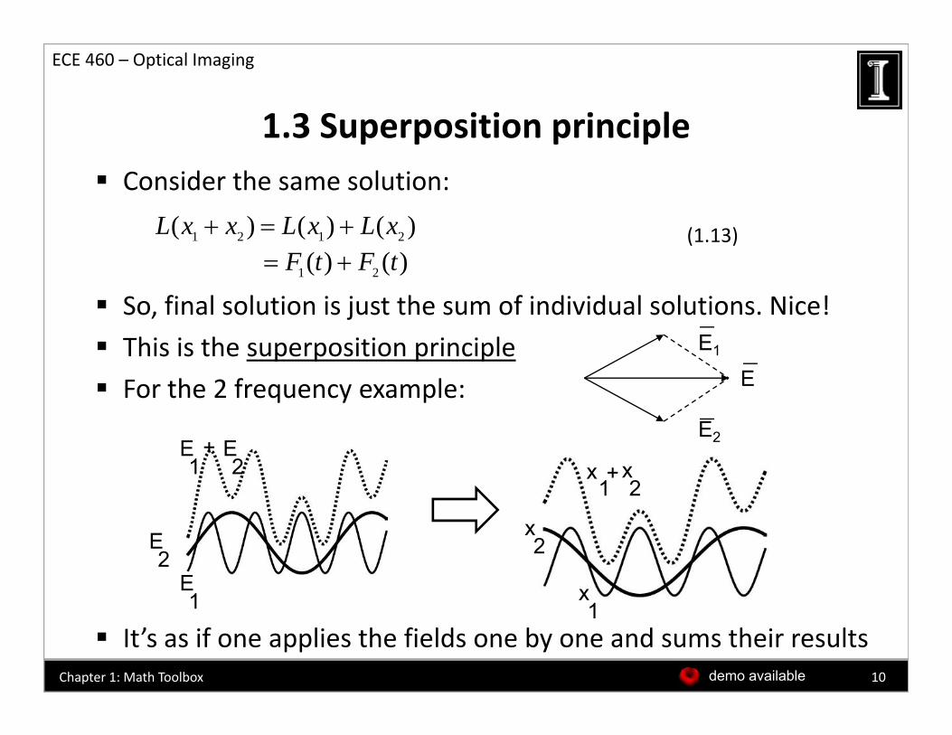
1.3 Superposition principle
ECE 460 – Optical Imaging
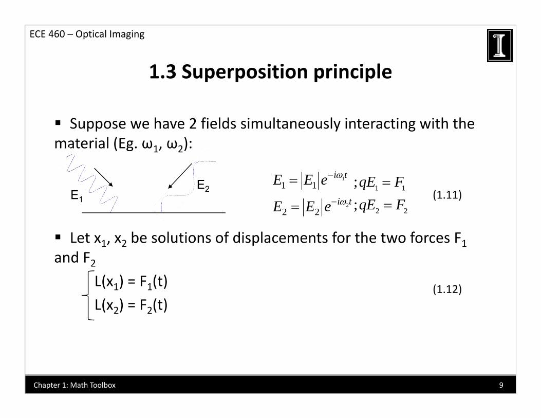
Suppose we have 2 fields simultaneously interacting with the
1.3 Superposition principle
pp y gmaterial (Eg. ω1, ω2):
11 1
i tE E e ;qE FE
Let x x be solutions of displacements for the two forces F
2
1 1
2 2i t
E E e
E E e 1 1
2 2
;;qE FqE F
(1.11)E1E2
Let x1, x2 be solutions of displacements for the two forces F1and F2
L(x1) = F1(t) (1 12)( 1) 1( )
L(x2) = F2(t)(1.12)
9Chapter 1: Math Toolbox
1.3 Superposition principle
ECE 460 – Optical Imaging
Consider the same solution:
1.3 Superposition principle
( ) ( ) ( )L x x L x L x (1 13)
So, final solution is just the sum of individual solutions. Nice!
1 2 1 2( ) ( ) ( )L x x L x L x
1 2( ) ( )F t F t (1.13)
This is the superposition principle
For the 2 frequency example: EE1
E2E1
E2
+
1x2
+x
E1
E2
x
x2
It’s as if one applies the fields one by one and sums their results1 x
1
10demo availableChapter 1: Math Toolbox
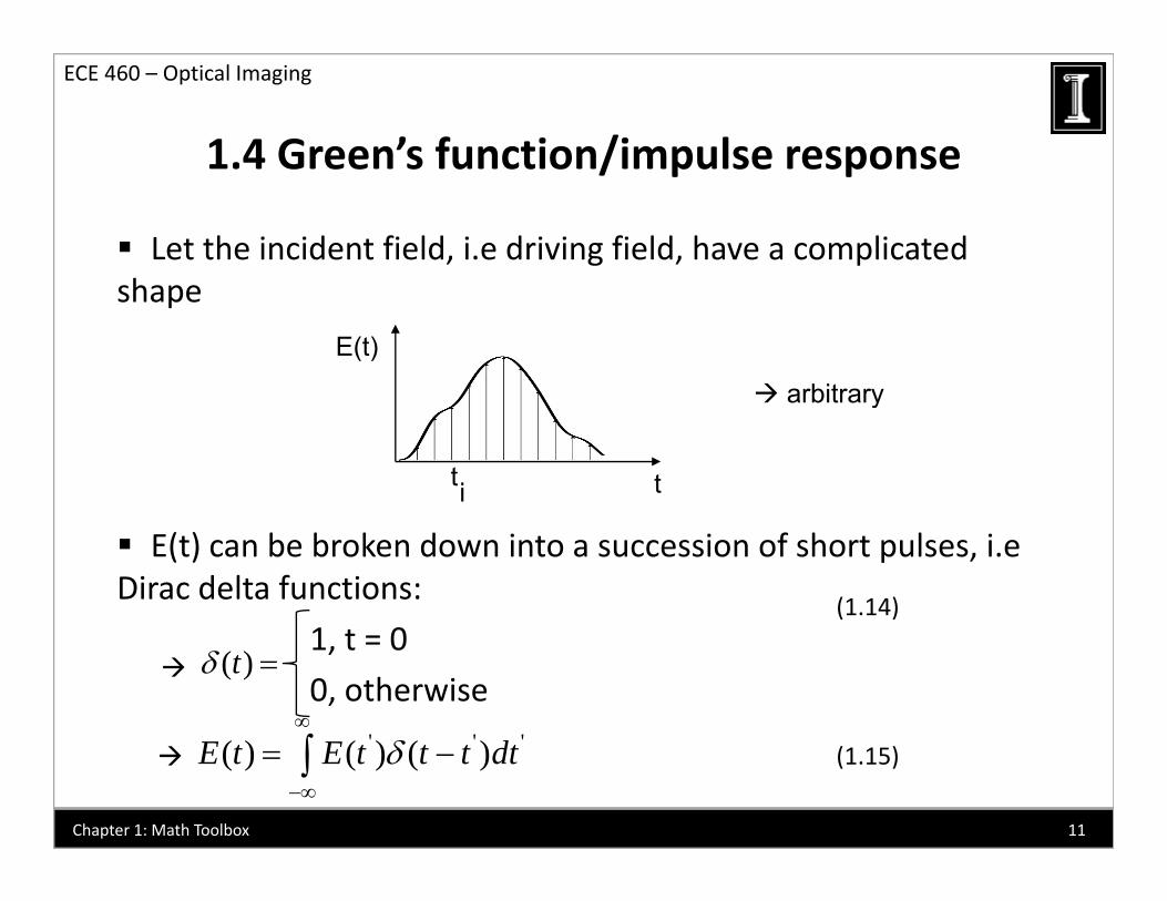
1.4 Green’s function/impulse response
ECE 460 – Optical Imaging
Let the incident field, i.e driving field, have a complicated h
1.4 Green s function/impulse response
shape
arbitrary
E(t)
arbitrary
tti
E(t) can be broken down into a succession of short pulses, i.e Dirac delta functions:
(1.14)1, t = 0
0, otherwise( )t
' ' '
' ' '( ) ( ) ( )E t E t t t dt
(1.15)
11Chapter 1: Math Toolbox
1.4 Green’s function/impulse response
ECE 460 – Optical Imaging
If we know the response of the system to a short pulse, ,
1.4 Green s function/impulse response
( )tp y p , ,the problem is solved
Let h(t) be the solution to
( )
( )t The final solution for an arbitrary force is:( ) ( )F t qE t
' ' '( ) ( ) ( )x t E t h t t dt
(1.16)
This is the Green’s method of solving linear problems
h(t) = Green’s function or impulse response of the system
h(t) Green s function or impulse response of the system
Complicated problems become easily tractable!
12Chapter 1: Math Toolbox
1.5 Fourier Transforms
ECE 460 – Optical Imaging
Very efficient tool for analyzing linear (and non‐linear) processes
1.5 Fourier Transforms
Definition: 2[ ( )] ( ) xi xff x f x e dx
( ) ( )F f f
(1.17)
F is the Fourier transform of f
f must satisfy:
( ) ( )xF f f
: ;f ( , , ) ( , , )x y z , f must satisfy:a) - modulus integrableb) f has finite number of discontinuities in the finite
: ;f f
( , , ) ( , , )y
)domainc) f has no infinite discontinuities
I i f h di i i
In practice, some of these conditions are sometimes relaxed
13demo availableChapter 1: Math Toolbox
1.5 Fourier Transforms
ECE 460 – Optical Imaging
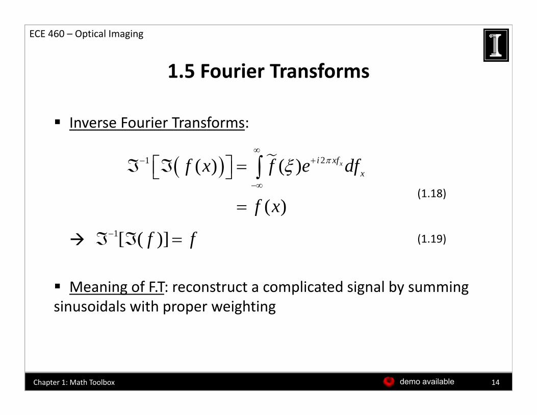
Inverse Fourier Transforms:
1.5 Fourier Transforms
21 ( ) ( ) xi xfxf x f e df
( )f x(1.18)
1[ ( )]f f
Meaning of FT: reconstruct a complicated signal by summing
1[ ( )]f f (1.19)
Meaning of F.T: reconstruct a complicated signal by summing sinusoidals with proper weighting
14demo availableChapter 1: Math Toolbox
1.5 Fourier Transforms
ECE 460 – Optical Imaging
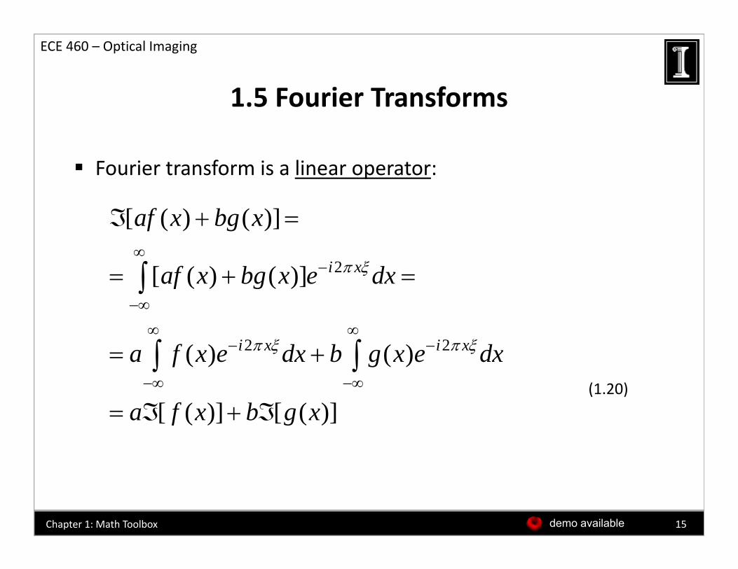
Fourier transform is a linear operator:
1.5 Fourier Transforms
p
[ ( ) ( )]af x bg x
2[ ( ) ( )] i xaf x bg x e dx
2 2( ) ( )i x i xa f x e dx b g x e dx
(1.20)
[ ( )] [ ( )]a f x b g x (1.20)
15demo availableChapter 1: Math Toolbox
1.6 Basic Theorems with Fourier Transforms
ECE 460 – Optical Imaging
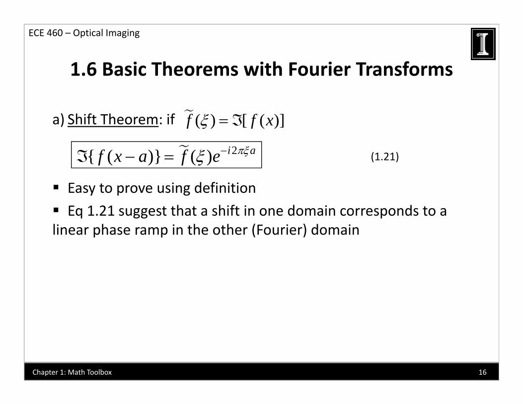
a) Shift Theorem: if
1.6 Basic Theorems with Fourier Transforms
( ) [ ( )]f f x )
(1.21)
( ) [ ( )]f f
2{ ( )} ( ) i af x a f e
Easy to prove using definition
Eq 1.21 suggest that a shift in one domain corresponds to a linear phase ramp in the other (Fourier) domainlinear phase ramp in the other (Fourier) domain
16Chapter 1: Math Toolbox
1.6 Basic Theorems with Fourier Transforms
ECE 460 – Optical Imaging
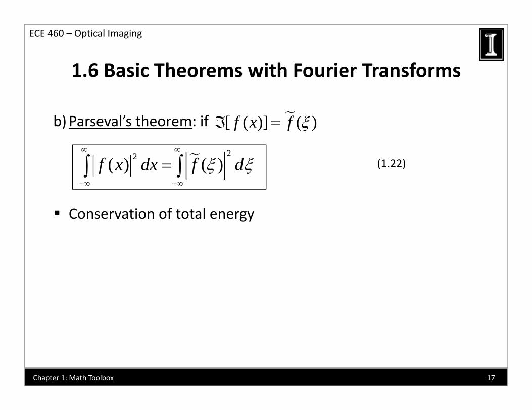
b)Parseval’s theorem: if
1.6 Basic Theorems with Fourier Transforms
[ ( )] ( )f x f )
(1.22)
[ ( )] ( )f x f
22( ) ( )f x dx f d
Conservation of total energy
17Chapter 1: Math Toolbox

1.6 Basic Theorems with Fourier Transforms
ECE 460 – Optical Imaging
c) Similarity theorem: if
1.6 Basic Theorems with Fourier Transforms
) y
, i.e. is the F.T of [ ( )] ( )xf x f f
1
f f
(1.23)1[ ( )]| |
f ax fa a
Theorem 1.23 provides intuitive feeling for F.T
Let’s consider
18Chapter 1: Math Toolbox
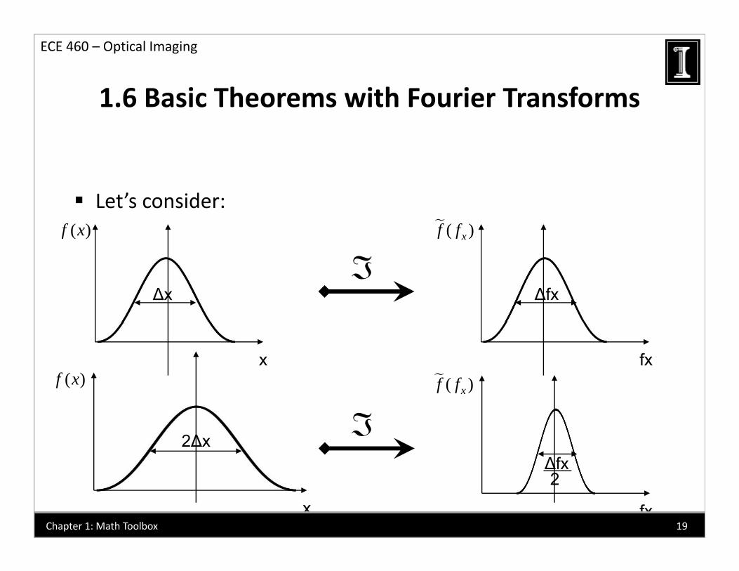
1.6 Basic Theorems with Fourier Transforms
ECE 460 – Optical Imaging
c) Similarity theorem:
1.6 Basic Theorems with Fourier Transforms
) y
Let’s consider:( )xf f( )f x
( )
ΔfxΔx
(Figures pageII‐8)x fx
( )xf f( )f x
Δfx
x
2Δx
x fx
Δfx2
19Chapter 1: Math Toolbox
1.6 Basic Theorems with Fourier Transforms
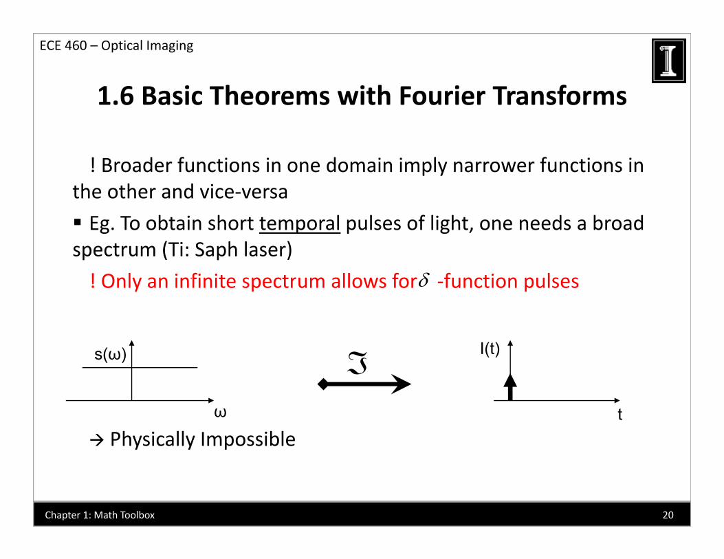
ECE 460 – Optical Imaging
! Broader functions in one domain imply narrower functions in
1.6 Basic Theorems with Fourier Transforms
p ythe other and vice‐versa
Eg. To obtain short temporal pulses of light, one needs a broad t (Ti S h l )spectrum (Ti: Saph laser)
! Only an infinite spectrum allows for ‐function pulses
s(ω) I(t)
Physically Impossibleω t
20Chapter 1: Math Toolbox
1.6 Basic Theorems with Fourier Transforms
ECE 460 – Optical Imaging
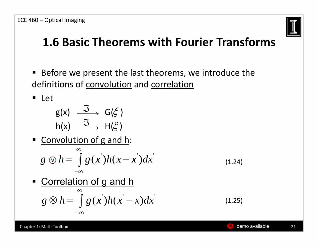
Before we present the last theorems, we introduce the
1.6 Basic Theorems with Fourier Transforms
p ,definitions of convolution and correlation
Let g(x) G( )
h(x) H( ) Convolution of g and h:
Convolution of g and h:
' ' '( ) ( )g h g x h x x dx
(1.24)
Correlation of g and h
' ' '( ) ( )g h g x h x x dx
(1 25)( ) ( )g h g x h x x dx
(1.25)
21demo availableChapter 1: Math Toolbox
1.6 Basic Theorems with Fourier Transforms
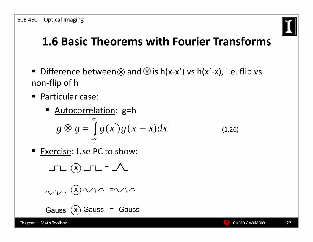
ECE 460 – Optical Imaging
Difference between and is h(x‐x’) vs h(x’‐x), i.e. flip vs
1.6 Basic Theorems with Fourier Transforms
v ( ) ( ), pnon‐flip of h
Particular case:
Autocorrelation: g=h
(1.26)' ' '( ) ( )g g g x g x x dx
Exercise: Use PC to show:
x =(Figures page II‐9)
x =
=x
Gauss x Gauss = Gauss
22demo availableChapter 1: Math Toolbox
1.6 Basic Theorems with Fourier Transforms
ECE 460 – Optical Imaging
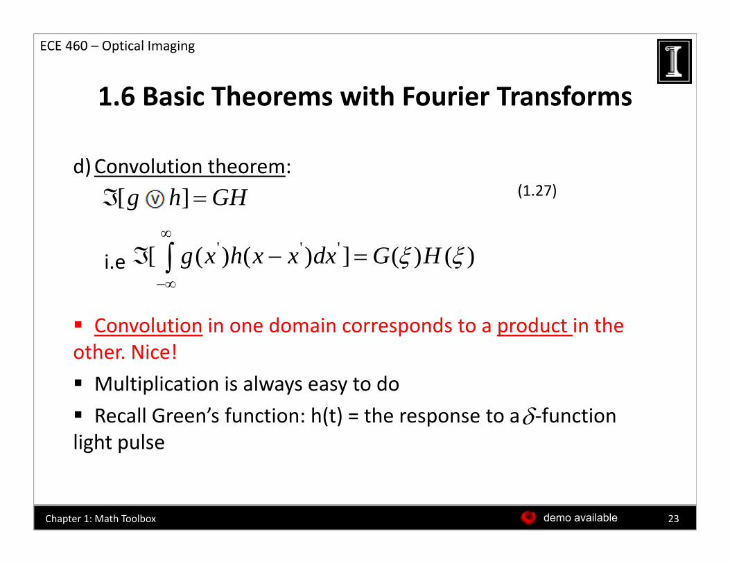
d)Convolution theorem:
1.6 Basic Theorems with Fourier Transforms
)
[ ]g h GH v (1.27)
' ' '
i.e' ' '[ ( ) ( ) ] ( ) ( )g x h x x dx G H
Convolution in one domain corresponds to a product in the other. Nice!
Multiplication is always easy to doMultiplication is always easy to do
Recall Green’s function: h(t) = the response to a ‐function light pulse
23demo availableChapter 1: Math Toolbox
1.6 Basic Theorems with Fourier Transforms
ECE 460 – Optical Imaging
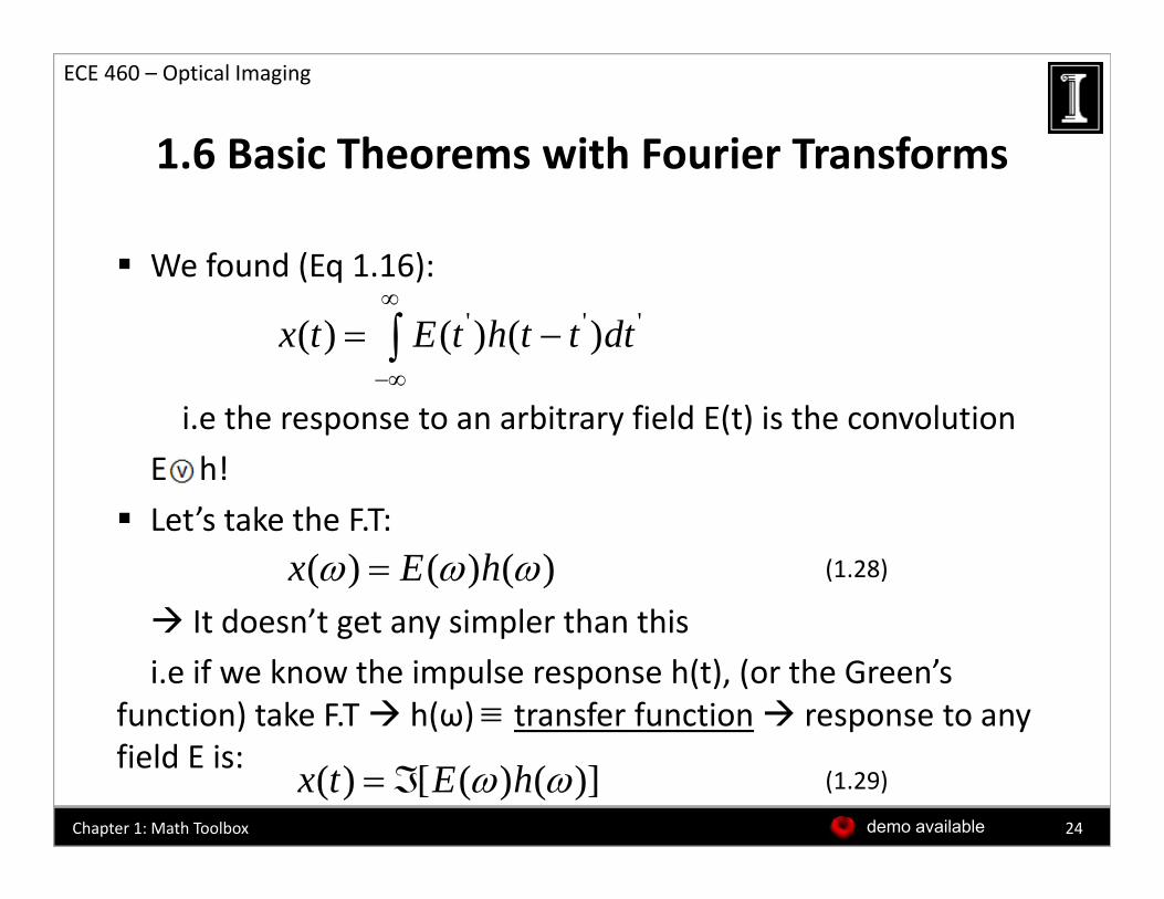
We found (Eq 1.16):
1.6 Basic Theorems with Fourier Transforms
( q )
' ' '( ) ( ) ( )x t E t h t t dt
i.e the response to an arbitrary field E(t) is the convolution
E h!
Let’s take the F.T:
It doesn’t get any simpler than this
( ) ( ) ( )x E h (1.28)
It doesn t get any simpler than thisi.e if we know the impulse response h(t), (or the Green’s
function) take F.T h(ω) transfer function response to any field E is: ( ) [ ( ) ( )]x t E h (1.29)
24demo availableChapter 1: Math Toolbox
1.6 Basic Theorems with Fourier Transforms
ECE 460 – Optical Imaging
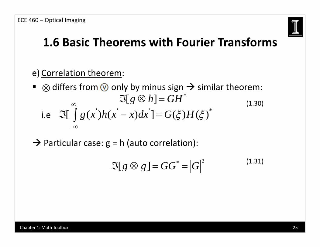
e) Correlation theorem:
1.6 Basic Theorems with Fourier Transforms
)
differs from only by minus sign similar theorem:
(1.30)*[ ]g h GH
i.e
' ' ' *[ ( ) ( ) ] ( ) ( )g x h x x dx G H
Particular case: g = h (auto correlation):
2*[ ]g g GG G (1.31)[ ]g g
25Chapter 1: Math Toolbox

1.6 Basic Theorems with Fourier Transforms
ECE 460 – Optical Imaging
e) Correlation theorem:
1.6 Basic Theorems with Fourier Transforms
)
Eg: F.T of an auto correlation is the power spectrum
Very important for both time and space fluctuating fields:
( ) ( ') ( ' )t E t E t t dt
*[ ( )] ( ) ( ) ( )E E S
= auto correlation
t(1.32)
We’ll meet them again later!
*[ ( )] ( ) ( ) ( )t E E S = power spectrum(Wiener–Khinchin theorem)
We ll meet them again later!
26Chapter 1: Math Toolbox
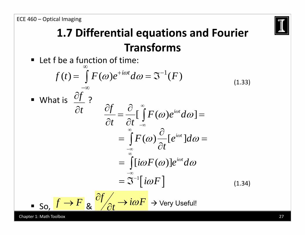
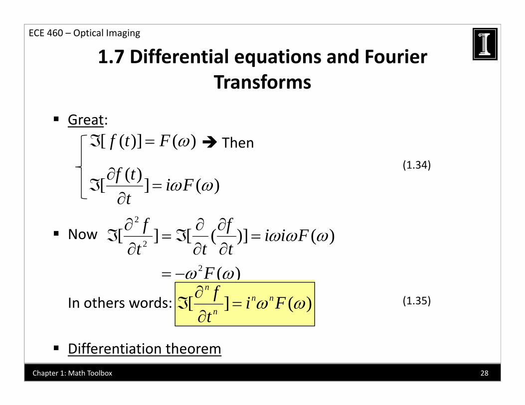
1.7 Differential equations and Fourier f
ECE 460 – Optical Imaging
Let f be a function of time:Transforms
1( ) ( ) ( )i tf F d F
What is ?
1( ) ( ) ( )i tf t F e d F
(1.33)
fWhat is ?t [ ( ) ]i tf F e d
t t
( ) [ ]i tF e d
t
[ ( )] i ti F e d
[ ( )]i F e d
(1.34) 1 i F
So, & f F f i Ft 27Chapter 1: Math Toolbox
Very Useful!
1.7 Differential equations and Fourier f
ECE 460 – Optical Imaging
Great:
Transforms
Then[ ( )] ( )f t F
( )f t(1.34)( )[ ] ( )f t i F
t
2 f f Now
2[ ] [ ( )] ( )f f i i Ft t t
2 ( )F
In others words:
( )
[ ] ( )n
n nn
f i Ft
(1.35)
Differentiation theorem28Chapter 1: Math Toolbox
1.7 Differential equations and Fourier f
ECE 460 – Optical Imaging
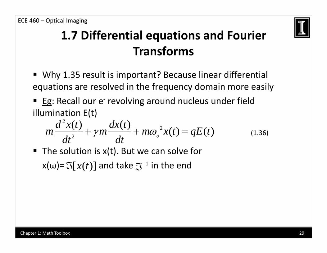
Why 1.35 result is important? Because linear differential
Transforms
y pequations are resolved in the frequency domain more easily
Eg: Recall our e‐ revolving around nucleus under field ill i ti E(t)illumination E(t)
22
2
( ) ( ) ( ) ( )o
d x t dx tm m m x t qE tdt dt
(1.36)
The solution is x(t). But we can solve for
x(ω)= and take in the end
dt dt
[ ( )]x t 1
29Chapter 1: Math Toolbox
1.7 Differential equations and Fourier f
ECE 460 – Optical Imaging
So, let’s take F.T of 1.36, using the differentiation
Transforms
, , gtheorem:
2 2[ ( )] ( ) ( ) ( )om x i mx m x qE
Since q= e:
2 2
[ ( )] ( ) ( ) ( )( )[ ] ( )
o
o
qx m i m m qE
Since q=-e:( )
( )
e Emx
(1.37)
2 2( )o
xi
30Chapter 1: Math Toolbox

1.7 Differential equations and Fourier f
ECE 460 – Optical Imaging
Exercise: use PC to take of Eq. 1.37
Transforms1 q
“damped” oscilation = damping factor damped oscilation, = damping factor! Problem solved
31Chapter 1: Math Toolbox
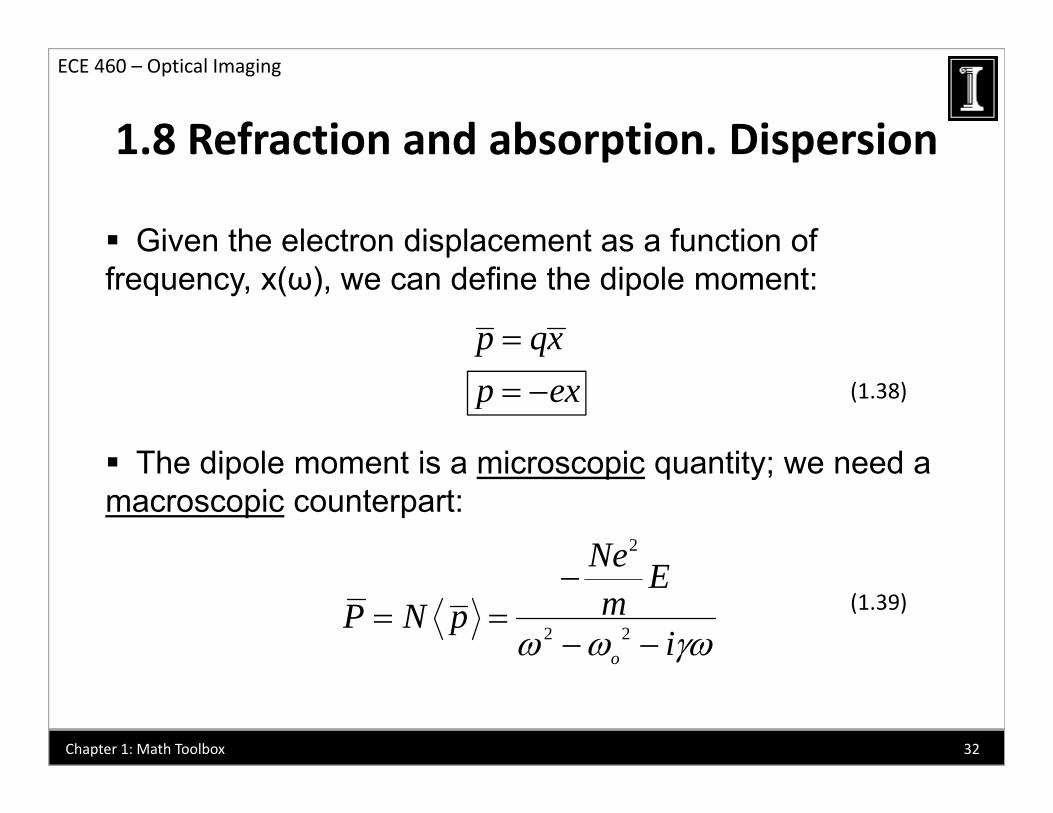
1.8 Refraction and absorption. Dispersion
ECE 460 – Optical Imaging
Given the electron displacement as a function of
1.8 Refraction and absorption. Dispersion
pfrequency, x(ω), we can define the dipole moment:
p qx
The dipole moment is a microscopic quantity; we need a
p qp ex (1.38)
The dipole moment is a microscopic quantity; we need a macroscopic counterpart:
2Ne
2 2o
Ne EmP N p
i
(1.39)
o
32Chapter 1: Math Toolbox
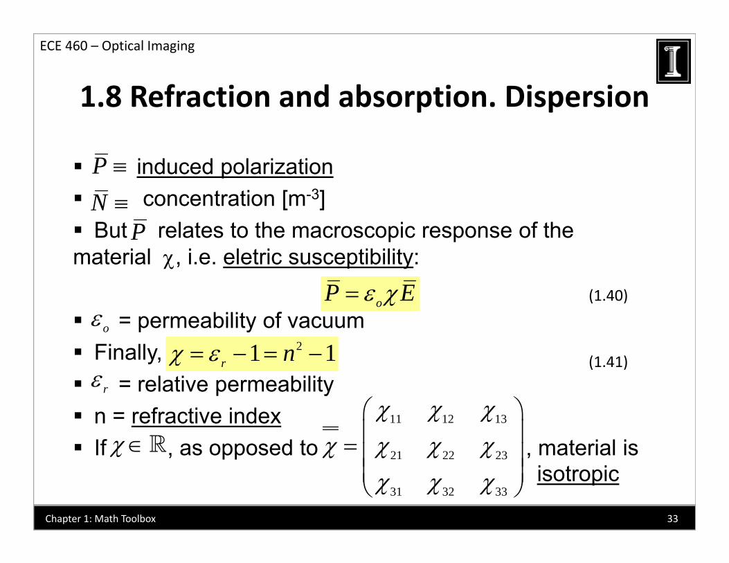
1.8 Refraction and absorption. Dispersion
ECE 460 – Optical Imaging
induced polarization
1.8 Refraction and absorption. Dispersion
P p concentration [m-3] But relates to the macroscopic response of the
N P
material , i.e. eletric susceptibility:
= permeability of vacuumoP E (1.40)
= permeability of vacuum Finally, = relative permeability
o21 1r n
r(1.41)
relative permeability n = refractive index If , as opposed to , material is
r
11 12 13
21 22 23
ppisotropic
3
31 32 33
33Chapter 1: Math Toolbox
1.8 Refraction and absorption. Dispersion
ECE 460 – Optical Imaging
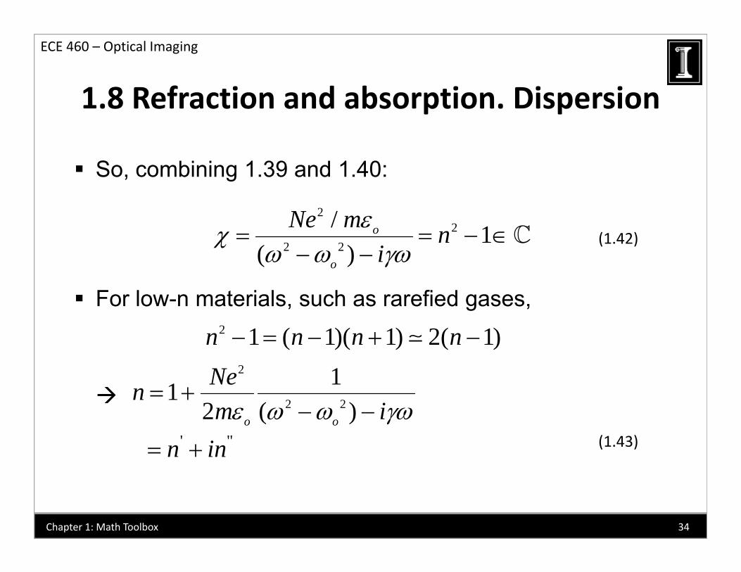
So, combining 1.39 and 1.40:
1.8 Refraction and absorption. Dispersion
, g
22
2 2
/ 1( )
oNe m ni
(1.42)
For low-n materials, such as rarefied gases,
2 2( )o i
2 1 ( 1)( 1) 2( 1)n n n n 2 11 Nen 2 21
2 ( )o o
nm i
' "n in (1.43)
34Chapter 1: Math Toolbox
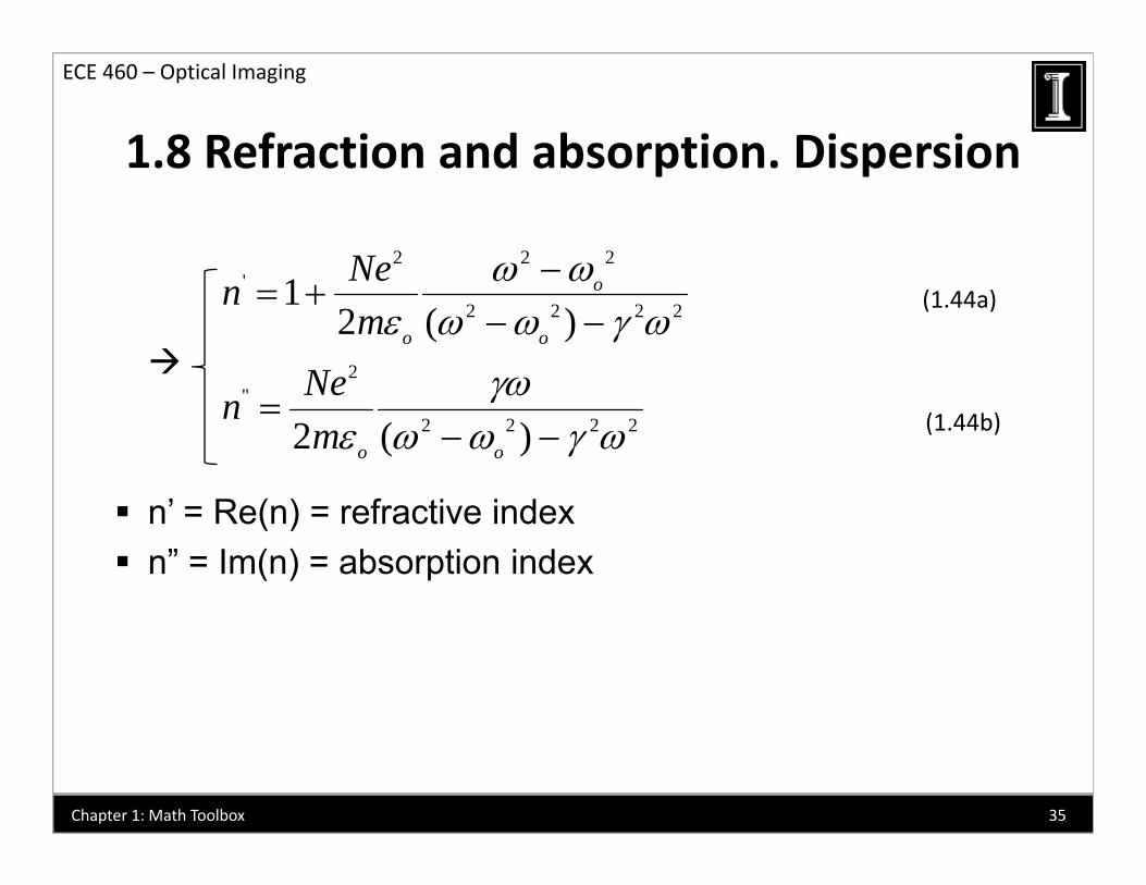
1.8 Refraction and absorption. Dispersion
ECE 460 – Optical Imaging
1.8 Refraction and absorption. Dispersion
2 2 2' Ne
'2 2 2 2
2
12 ( )
o
o o
Nenm
Ne
(1.44a)
’ ( ) f
(1.44b)"
2 2 2 22 ( )o o
Nenm
n’ = Re(n) = refractive index n” = Im(n) = absorption index
35Chapter 1: Math Toolbox
1.8 Refraction and absorption. Dispersion
ECE 460 – Optical Imaging
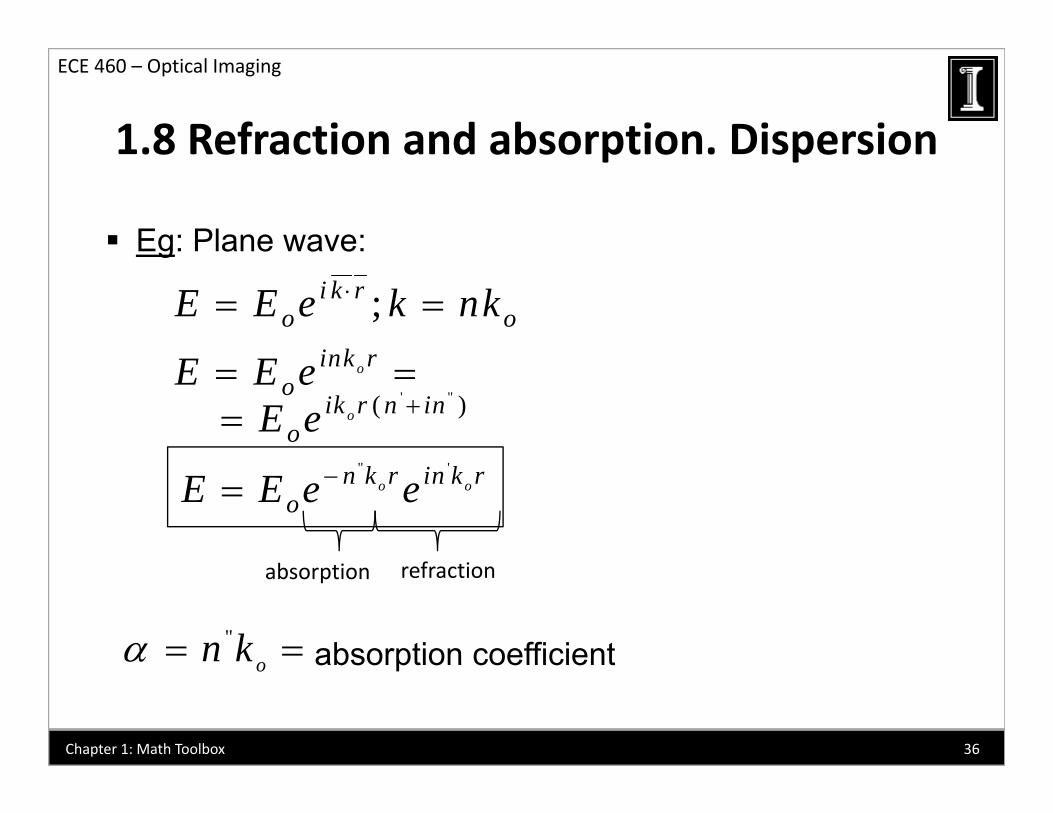
Eg: Plane wave:
1.8 Refraction and absorption. Dispersion
g
;i k ro o
ink r
E E e k nk oink r
oE E e ' "( )oik r n in
oE e " '
o on k r in k roE E e e
absorption coefficient
absorption refraction
"on k absorption coefficiento
36Chapter 1: Math Toolbox
1.8 Refraction and absorption. Dispersion
ECE 460 – Optical Imaging
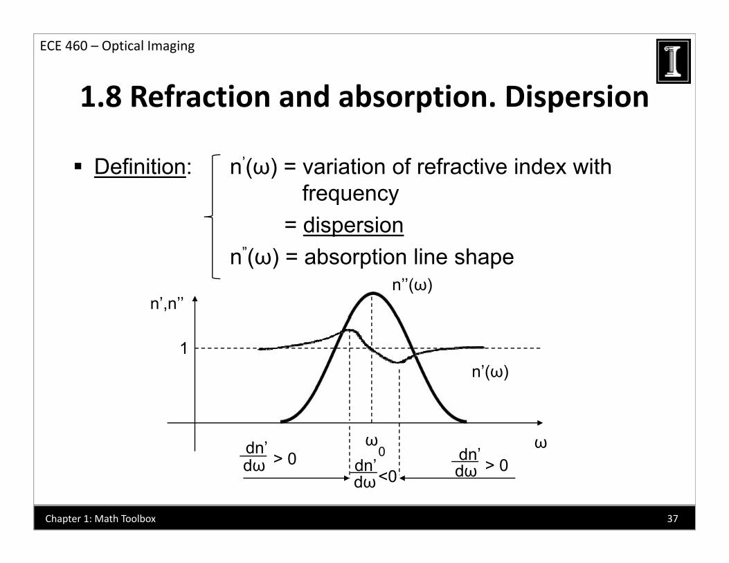
Definition: n’(ω) = variation of refractive index with
1.8 Refraction and absorption. Dispersion
( )frequency
= dispersionn”(ω) = absorption line shape
n’,n’’n’’(ω)
(Figure page II-16) 1n’(ω)
ωω0 dn’
d > 0 0dn’
d ’dn
dω > 0dω > 0dn’
dω<0
37Chapter 1: Math Toolbox

1.8 Refraction and absorption. Dispersion
ECE 460 – Optical Imaging
Note the line shape:
1.8 Refraction and absorption. Dispersion
p
2 22 2 2 2
1 1 1 1( ) ( )2
f
( ) ( )21 1/ 2
o o o o
o
Lorentz function:
; a = width1 1( )
; a = width2( )1 ( / )a a
38Chapter 1: Math Toolbox
1.8 Refraction and absorption. Dispersion
ECE 460 – Optical Imaging
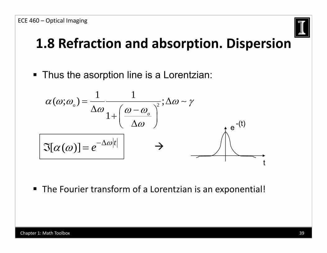
Thus the asorption line is a Lorentzian:
1.8 Refraction and absorption. Dispersion
p
2
1 1( ; ) ;o
1 o
t
e -(t)
[ ( )] te t
The Fourier transform of a Lorentzian is an exponential!
39Chapter 1: Math Toolbox
1.8 Refraction and absorption. Dispersion
ECE 460 – Optical Imaging
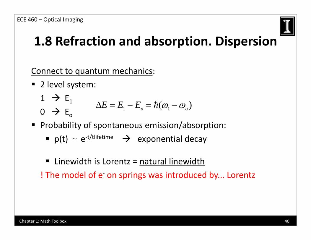
Connect to quantum mechanics:
1.8 Refraction and absorption. Dispersion
q
2 level system:
1 E1 ( )E E E 0 Eo
Probability of spontaneous emission/absorption:/ lif i
1 1( )o oE E E
p(t) e‐t/tlifetime exponential decay
Linewidth is Lorentz = natural linewidth
! The model of e‐ on springs was introduced by... Lorentz
40Chapter 1: Math Toolbox
1.9 Maxwell’s Equations
ECE 460 – Optical Imaging
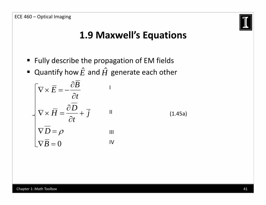
Fully describe the propagation of EM fields
1.9 Maxwell s Equations
y p p g
Quantify how and generate each otherE HBE
IEt
DH j
II (1.45a)
0
jt
DB
III
IV
(1.45a)
0B IV
41Chapter 1: Math Toolbox
1.9 Maxwell’s Equations
ECE 460 – Optical Imaging
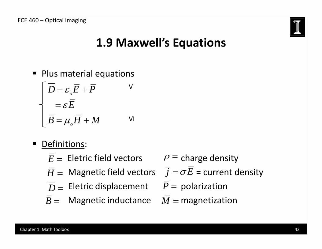
Plus material equations
1.9 Maxwell s Equations
q
oD E P
E
V
oB H M VI
Definitions:
Eletric field vectors charge density
Magnetic field vectors = current densityE H
j EMagnetic field vectors = current density
Eletric displacement polarization
Magnetic inductance magnetization
H D
B
j EP M Magnetic inductance magnetizationB M
42Chapter 1: Math Toolbox
1.9 Maxwell’s Equations
ECE 460 – Optical Imaging
Let’s combine I and II (assume no free charge: = 0, =0)
1.9 Maxwell s Equations
j( g , )
Use property:
Since
j2( ) ( )E E E
20 0 ( )E E E
Take ( ) :EqI
( ) BEt
(1.46)
t 2 ( )E B
t
( )o Ht
(see next slide)
( )ot t
43Chapter 1: Math Toolbox
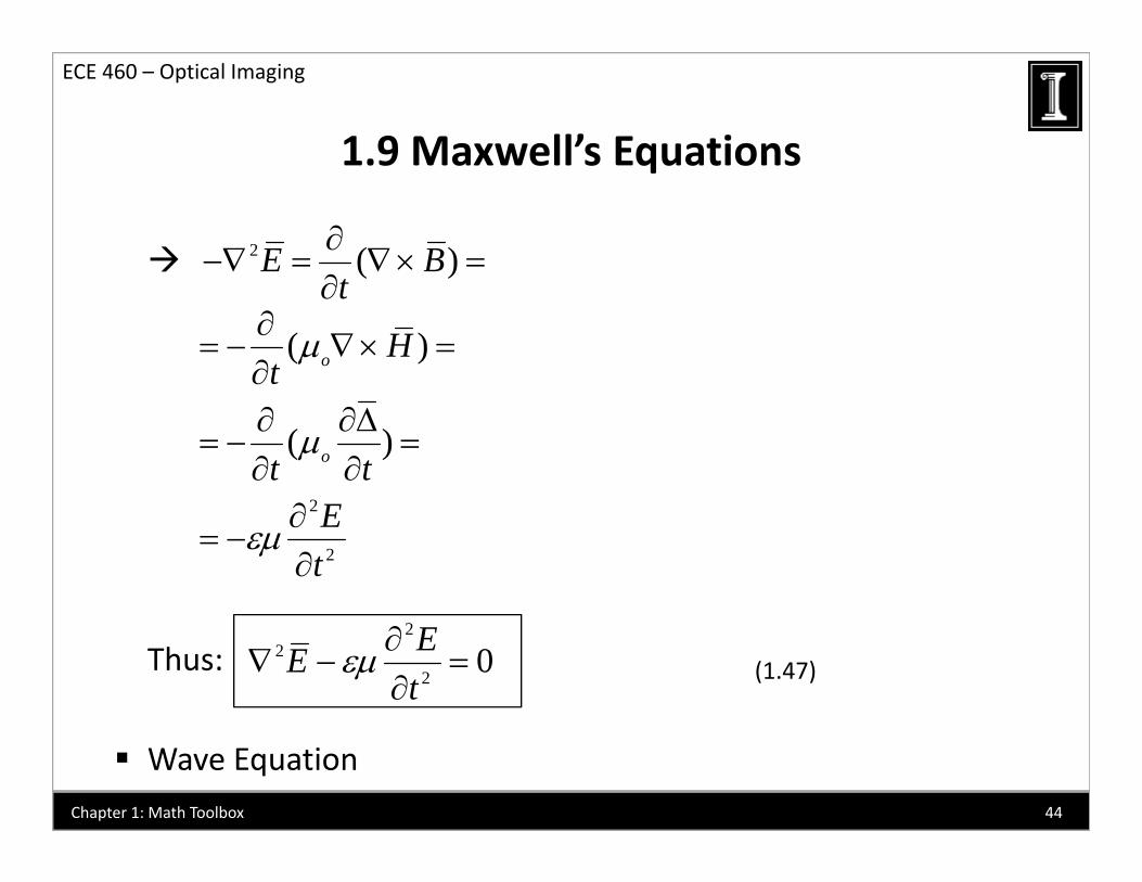
1.9 Maxwell’s Equations
ECE 460 – Optical Imaging
1.9 Maxwell s Equations
2 ( )E B
( )o Ht
( )t
( )ot t
2
2
Et
Thus:2
22
0EEt
(1.47)
Wave Equation44Chapter 1: Math Toolbox
1.9 Maxwell’s Equations
ECE 460 – Optical Imaging
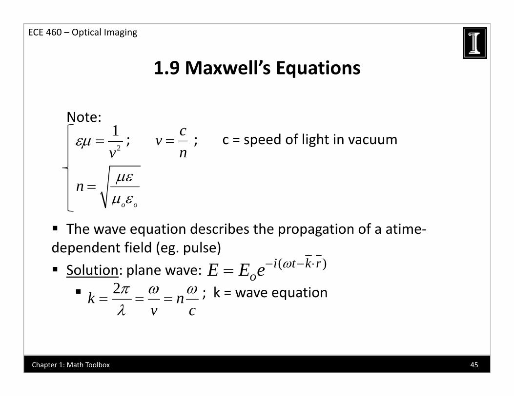
Note:
1.9 Maxwell s Equations
; ; c = speed of light in vacuum2
1v
cvn
o o
n
The wave equation describes the propagation of a atime‐dependent field (eg. pulse)
Solution: plane wave: ( )i t k rE E e Solution: plane wave:
; k = wave equationoE E e
2k nv c
45Chapter 1: Math Toolbox
1.9 Maxwell’s Equations
ECE 460 – Optical Imaging
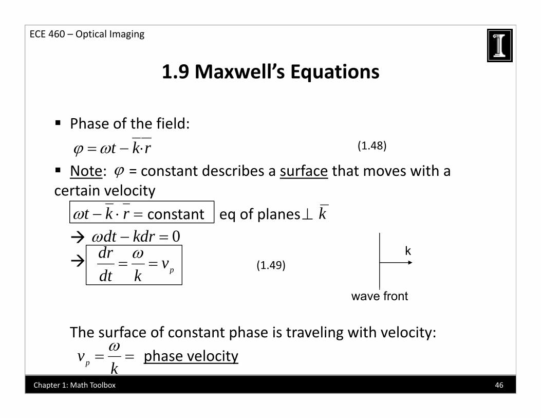
Phase of the field:
1.9 Maxwell s Equations
Note: = constant describes a surface that moves with a t k r
(1.48)
certain velocity
constant eq of planes
t k r k0dt kdr
0dt kdr
p
dr vdt k
(1.49)
k
The surface of constant phase is traveling with velocity:
wave front
phase velocitypvk
46Chapter 1: Math Toolbox
1.9 Maxwell’s Equations
ECE 460 – Optical Imaging
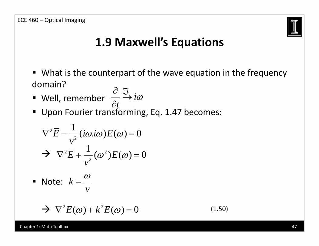
What is the counterpart of the wave equation in the frequency
1.9 Maxwell s Equations
p q q ydomain?
Well, remember it
Upon Fourier transforming, Eq. 1.47 becomes:
22
1 ( . ) ( ) 0E i i E
2v2 2
2
1 ( ) ( ) 0E Ev
Note: kv
2 2( ) ( ) 0E k E (1.50)
47Chapter 1: Math Toolbox

1.9 Maxwell’s Equations
ECE 460 – Optical Imaging
1.9 Maxwell s Equations
2 2( ) ( ) 0E k E The equation above is the “Helmholtz equation”
Describes how each frequency ω propagates
( ) ( )
48Chapter 1: Math Toolbox