chapter 11 scalability and distribution of collaborative …chri2951/chapter11.pdf ·...

September 19, 2018 14:15 ws-rv9x6-9x6 Book Title 11131-11 page 375

Chapter 11

Scalability and Distribution ofCollaborative Recommenders

Evangelia Christakopoulou

Computer Science & EngineeringUniversity of Minnesota, Minneapolis, MN

[email protected]

Shaden Smith


[email protected]

Mohit Sharma


[email protected]

Alex Richards

Department of Computer EngineeringSan Jose State [email protected]

David Anastasiu

Department of Computer EngineeringSan Jose State [email protected]

George Karypis


[email protected]

375


376 E. Christakopoulou et al.

Recommender systems are ubiquitous; they are foundational to a widevariety of industries ranging from media companies such as Netflix to e-commerce companies such as Amazon. As recommender systems continueto permeate the marketplace, we observe two major shifts which must beaddressed. First, the amount of data used to provide quality recommen-dations grows at an unprecedented rate. Secondly, modern computer ar-chitectures display great processing capabilities that significantly outpacememory speeds. These two trend shifts must be taken into account in orderto design recommendation systems that can e�ciently handle the amountof available data by distributing computations in order to take advantageof modern parallel architectures. In this chapter, we present ways to scalepopular collaborative recommendation methods via parallel computing.

11.1. Introduction

Recommender systems are ubiquitous; they are foundational to a widevariety of industries ranging from media companies such as Netflix to e-commerce companies such as Amazon. Their popularity is attributed totheir ability to e↵ectively navigate users through a plethora of productoptions which would otherwise go unexplored. As recommender systemscontinue to permeate the marketplace, we observe two major shifts whichmust be addressed.

First, the amount of data used to provide quality recommendationsgrows at an unprecedented rate. For example, companies such as Netflixstream millions of movies each day. Secondly, modern computer archi-tectures forego great changes. The last two decades have seen availableprocessing capabilities significantly outpace memory speeds. This disparityhas shifted the cost of many computations from mathematical operationsto data movements. In consequence, algorithm designers must now exposelarge amounts of parallelism while reducing data movement costs. Thesetwo trend shifts must be taken into account in order to design recommen-dation systems that can e�ciently handle the amount of available data bydistributing computations in order to take advantage of modern parallelarchitectures.

Unfortunately, designing successful recommendation systems that cane↵ectively utilize modern parallel architectures is not always straightfor-ward. Most popular recommendation algorithms are inherently unstruc-tured, meaning that data accesses are not known apriori because they aredetermined by the structure of the input data. The unstructured nature of


Scalability and Distribution of Collaborative Recommenders 377

the underlying computations is further complicated by non-uniform distri-butions exhibited by real-world ratings datasets. A small number of popularitems and prolific users cause the data to follow a power-law distribution,which presents challenges when partitioning work to processing cores in abalanced manner.

In this chapter, we present ways to scale popular collaborative recom-mendation methods via parallel computing. The methods we present spanboth of the primary recommendation tasks: the top-N recommendationtask, where we are interested in whether a user will likely purchase an item,and the rating prediction task, which focuses on determining how much auser would enjoy a product. The nearest neighbor methods presented inSection 11.2 are used for both tasks. The sparse linear methods presentedin Section 11.3 are oriented towards the top-N recommendation task. Fi-nally, the matrix and tensor factorization methods presented in Section 11.4can be used for both tasks, but for the purposes of this chapter, they areprimarily viewed in the context of rating prediction.

The presented methods are very di↵erent from each other and exhibitdi↵erent parallelization opportunities. For each method, an overview ispresented, along with a discussion of how it can be scaled and experimentalresults showing the runtimes and speedup achieved on the MovieLens 10M(ML10M) dataset.

The rest of the chapter has the following structure: Subsections 11.1.1and 11.1.2 present the notation and evaluation methodology used in therest of the chapter. Section 11.2 presents methods to e�ciently identifyneighbors in the nearest-neighbor approaches. Section 11.3 describes sparselinear methods, where both the neighbors to a target item and their similar-ities are estimated through solving an optimization problem and discussestheir scalability. Finally, Section 11.4 gives an overview and discusses thee�ciency of matrix and tensor factorization approaches.

11.1.1. Notation

In the rest of the chapter, we will use bold capital letters to refer to matrices(e.g., A) and bold lower case letters to refer to vectors (e.g., p). The vectorsare assumed to be column vectors. Thus, ai refers to the ith column ofmatrix A and we will use the transpose (aT

i ) to describe row vectors.We note the rating matrix, which contains the feedback given by n users

to m items as R. The dimensions of R are n ⇥m. We will use the termu to note a user, and i to note an item. The rating given by a user u to



an item i will be noted by rui and with a slight abuse of notation will beused to show both the explicit rating that user u gave to item i and/or theimplicit feedback (purchase/like) from u to i. We will use the notation rui

to refer to the predicted rating. Finally, we use the notation | · | to refer tothe number of non-zeros in the corresponding matrix or vector.

11.1.2. Evaluation

Dataset Throughout this chapter, we will demonstrate the e�ciency ande↵ectiveness of di↵erent recommender methods using the MovieLens 10Million (ML10M) [Harper and Konstan (2015)] ratings dataset. ML10Mconsists of 10 million ratings provided to 10677 movies by 69878 users. Eachrating is accompanied by a timestamp. The timestamps span 158 monthsand are used in tensor factorization approaches in Section 11.4.

Evaluation In order to evaluate the performance of the methods, weemploy a leave-one-out validation scheme. For every user, we leave outone rating and we train the model on the rest of the user’ ratings. Allthe left-out ratings comprise the test set. We repeat this procedure threetimes, thus resulting in three folds (three train sets and three associatedtest sets). In the end, for every method, we report the average time takenand the average performance of the folds.

As the exact rating is not used in top-N methods, the implicit feedbackof the ML10M dataset is used instead in Section 11.3. In this scenario,non-zero rating values in R are replaced with 1s, signifying the existenceof a rating given by a user to an item in the original data. To evaluatetop-N recommendation methods, we need to investigate whether the itemof the user that belongs to the test set is included in the list of top-Nrecommendations to the user, and in which position. Therefore, we use twoperformance metrics: HR and ARHR, where:

HR =#hits

#users, (11.1)

and

ARHR =#hitsX

i=1

1

pi. (11.2)

The #hits denotes the number of times that the test items were includedin the top-N recommendation list and pi is the position of the test item inthe recommended list, with pi = 1 being the top position. In this chapter,



we have evaluated the top-N recommendation methods by computing HRand ARHR for N = 10.

In the rating prediction methods, the explicit ratings are used. Also,when presenting the tensor factorization methods in Section 11.4, the as-sociated timestamps are used beyond the ratings. To evaluate the ratingprediction methods, we need to see how similar or di↵erent the predictedvalues of the ratings are with the actual ratings. We employ the Root MeanSquared Error (RMSE) to do that:

RMSE =

sPu

Pi (rui � rui)2

|R|. (11.3)

More details on RMSE, HR, ARHR and other evaluation measures canbe found in Chapter 9. A thorough explanation of the di↵erence betweenexplicit and implicit feedback can be found in Chapter 7.

System characteristics For consistency and comparison purposes, allexperiments are executed on the same system1 consisting of identical nodesequipped with 64 GB RAM and two twelve-core 2.5 GHz Intel Xeon E5-2680v3 (Haswell) processors. Each core is equipped with 32 KB L1 cacheand 256 KB of L2 cache, and the 12 cores on each socket share 30 MB ofL3 cache.

11.2. Scaling up nearest-neighbor approaches

A number of recommender systems rely on finding nearest neighbors amongusers or items as an integral part of deriving recommendations or traininga predictive recommendation model. More details on nearest-neighbor ap-proaches can be found in Chapter 1. A neighbor is defined as a user/itemwho is similar to the target user/item, based on a similarity notion (e.g.the target user and the neighbor user have co-rated a lot of items). Thesymbol Ni(u) represents the set of neighbors of the item i rated by theuser u. Similarly, the symbol Nu(i) represents the set of neighbors of useru, who have rated item i. In this section, we discuss approaches to speedup neighborhood identification, which directly a↵ects recommendation ef-ficiency.

1https://www.msi.umn.edu/content/mesabi



11.2.1. Use of neighborhoods in Recommender Systems

Collaborative filtering based recommenders, such as the user-based neigh-borhood method [Konstan et al. (1997)] or item-based neighborhood meth-ods [Sarwar et al. (2001); Deshpande and Karypis (2004)], first identify aset of neighbors and then use the ratings associated with those neighborsto derive the predicted rating for the user in question. User-based methodsidentify a set of users similar to target user u and predict the rating of useru on item i as

rui = µu +

Pv2Nu(i)

sim(u, v)(rvi � µv)Pv2Nu(i)

sim(u, v),

where sim(u, v) denotes the similarity between the users u and v, and µu

and µv are the means of the ratings provided by users u and v, respectively.Item-based neighborhood methods, however, derive the rating of user u

on target item i by considering other items that have been rated (generallyhigh) by the user u. The predicted rating of u on i is given by

rui = µi +

Pj2Ni(u)

sim(i, j)(ruj � µj)Pj2Ni(u)

sim(i, j).

where sim(i, j) denotes the similarity between the items i and j, and µi

and µj are the means of the ratings received by items i and j, respectively.A number of di↵erent recommenders can be designed given di↵erent

choices in applying the formulas above with respect to user and item repre-sentations, similarity function, or neighborhood construction. The standardapproach is to represent user u as the sparse vector of ratings for items ratedby the user (row u in the ratings matrix R) and item i as the vector of allratings given to item i by users (column i in R). Given a vector represen-tation of users and items, the similarity between users or between items ismost often computed as the cosine similarity or Pearson correlation coef-ficient between their respective vectors. Finally, the neighborhoods Nu(i)and Ni(u) can be constructed by finding all neighbors with a similarityabove some minimum threshold ✏, or one may consider only the k closestneighbors to the target user or item.

Beyond deriving recommendations by relying on similar users or items,some optimization-based recommenders learn a recommendation model byfocusing only on the ratings of similar users or items during the learningprocess (e.g., the fs-SLIM model [Ning and Karypis (2011)]).



Naıve approaches will compare each user to every other user, thus lead-ing to quadratic complexity in the number of computed similarities. In theremainder of this section, we will discuss e�cient methods that identifynearest neighbors given user-item ratings. The methods rely on aggressivepruning of the search space by identifying pairs of users or items that can-not be similar enough based on theoretic upper bounds on their computedsimilarity. Additional performance gains are achieved via e�cient use ofthe memory hierarchy of modern computing systems and shared-memoryparallelism.

We focus our discussion on two nearest neighbor problems useful inthe recommender systems context. The ✏-nearest neighbor graph (✏NNG)construction problem, also known as all-pairs similarity search (APSS) orsimilarity join, identifies, for each user/item in a set, all other users/itemswith a similarity of at least ✏. On the other hand, the k-nearest neighborgraph (kNNG) construction constrains each identified neighborhood to thek users/items closest to the target user/item. To simplify the discussion,we will describe the methods in the context of constructing item neighbor-hoods. The same methods can be applied to find user-based neighbors.

11.2.2. ✏-nearest neighbor graph construction

Recently, several methods have been proposed that e�ciently constructthe ✏NNG by filtering (or ignoring) pairs of items that cannot be neighbors[Bayardo et al. (2007); Anastasiu and Karypis (2014, 2015b); Anastasiu(2017)]. Item rating profile vectors are inherently sparse, as few users mayconsume and rate each item. The proposed methods take advantage ofthis sparsity and use data structures and processing strategies designed toeliminate unnecessary memory accesses and multiplication operations. TheL2-norm All Pairs (L2AP) [Anastasiu and Karypis (2014)] and Parallel L2-norm All Pairs (pL2AP) [Anastasiu and Karypis (2015b)] methods con-struct an exact neighborhood graph, finding the same neighbors as thosefound by a brute-force method that compares each user/item against allother users/items. Cosine Approximate Nearest Neighbors (CANN) [Anas-tasiu (2017)], on the other hand, finds most but not necessarily all of theneighbors with a similarity of at least ✏.

These methods use an inverted index data structure to eliminate unnec-essary comparisons. The inverted index is represented by the sparse userrating profiles. It consists of a set of lists, one for each user, such thatthe uth list contains pairs (i, rui) for all items i that have a non-zero rui



rating. Many unnecessary memory accesses and similarity computationscan be avoided by only comparing an item against the set of items foundin the inverted index lists for the users that rated it. In this way, twoitems that have not been rated by any common user will never have theirsimilarity computed.

Additional savings can be achieved by taking advantage of the inputsimilarity threshold ✏. Note that cosine similarity measures the cosine ofthe angle between the two vectors and is thus independent of the vectorlengths. A standard preprocessing step in computing cosine similarity is tonormalize the vectors with respect to their L2-norm, which reduces com-puting the cosine similarity of two vectors to finding their dot-product. Themethods compute only part of the dot-product of profile vectors for mostpairs of items, e.g., using only the tail-end features in the profile vector.Several theoretic upper bounds of vector dot-products are used to estimatethe portion of the dot-product for the leading features. If the sum of theestimate and computed portions of the dot-product is below ✏, the itemscannot be similar enough and are pruned.

Many item comparisons are completely avoided through a partial index-ing strategy. Only a few of the leading features of the profile of an item i

are indexed, enough to ensure that any item j with a similarity of at least✏ will be found by traversing the partial index. This strategy leads to a twophase process for constructing the exact ✏NNG. First, partial similarities(dot-products) are computed using values stored in the inverted index listsfor users that rated item i, which are called candidates. In the second phase,the un-indexed portion of each of the candidate profile vectors is used tofinish computing similarities only for those items with non-zero similarityafter the first phase. In both phases, additional similarity upper-boundsare used to eliminate candidates that cannot be similar enough.

Parallelization of pL2AP focuses on a cache-tiling strategy that aims tofit critical data structures used during similarity search in the high-speedyet limited cache memory of the system. The method splits the set of itemssuch that each subset has a partial inverted index that can fit in cachememory. Each core is then assigned small sets of neighborhood searches for20 consecutive items, which could be independently executed. Additionally,a small-memory footprint hash table data structure is proposed which isuniquely suited to the memory access patterns in pL2AP and providesfast access to profile vector values and meta-data necessary for computingsimilarity upper bounds. Algorithm 1 provides a sketch of the pL2APprocessing pipeline. Additional details for the algorithm and the di↵erent



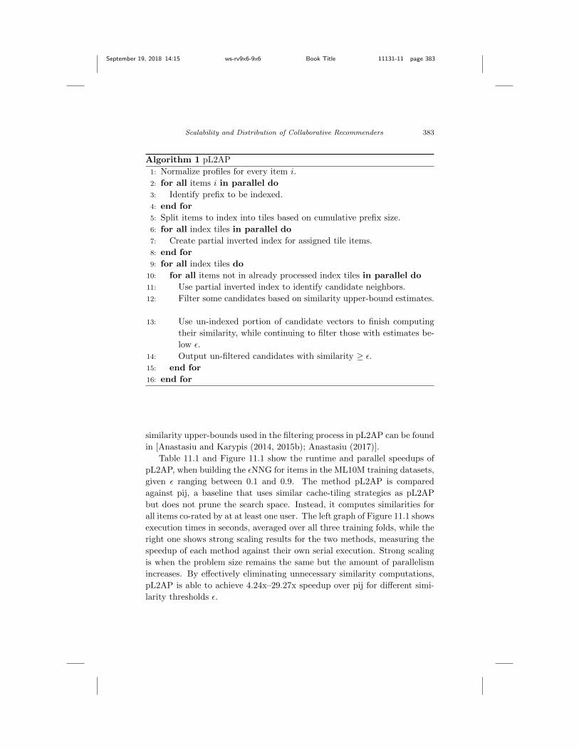
Algorithm 1 pL2AP

1: Normalize profiles for every item i.2: for all items i in parallel do3: Identify prefix to be indexed.4: end for5: Split items to index into tiles based on cumulative prefix size.6: for all index tiles in parallel do7: Create partial inverted index for assigned tile items.8: end for9: for all index tiles do

10: for all items not in already processed index tiles in parallel do11: Use partial inverted index to identify candidate neighbors.12: Filter some candidates based on similarity upper-bound estimates.

13: Use un-indexed portion of candidate vectors to finish computingtheir similarity, while continuing to filter those with estimates be-low ✏.

14: Output un-filtered candidates with similarity � ✏.15: end for16: end for

similarity upper-bounds used in the filtering process in pL2AP can be foundin [Anastasiu and Karypis (2014, 2015b); Anastasiu (2017)].

Table 11.1 and Figure 11.1 show the runtime and parallel speedups ofpL2AP, when building the ✏NNG for items in the ML10M training datasets,given ✏ ranging between 0.1 and 0.9. The method pL2AP is comparedagainst pij, a baseline that uses similar cache-tiling strategies as pL2APbut does not prune the search space. Instead, it computes similarities forall items co-rated by at at least one user. The left graph of Figure 11.1 showsexecution times in seconds, averaged over all three training folds, while theright one shows strong scaling results for the two methods, measuring thespeedup of each method against their own serial execution. Strong scalingis when the problem size remains the same but the amount of parallelismincreases. By e↵ectively eliminating unnecessary similarity computations,pL2AP is able to achieve 4.24x–29.27x speedup over pij for di↵erent simi-larity thresholds ✏.



Table 11.1. Runtime and speedup of pL2AP over pij on the ML10M dataset, when

executed using 24 cores.

Method ✏ = 0.1 0.2 0.3 0.4 0.5 0.6 0.7 0.8 0.9

time (s)

pij 3.22 3.22 3.22 3.22 3.22 3.22 3.22 3.23 3.22

pL2AP 0.76 0.55 0.42 0.34 0.26 0.21 0.15 0.13 0.11

speedup

pL2AP 4.24 5.85 7.67 9.38 12.38 15.60 21.47 24.82 29.27

Fig. 11.1. Runtime (left) and strong scaling (right) of pL2AP and the naıve baseline

pij when executed on the ML10M dataset.

11.2.3. k-nearest neighbor graph construction

One potential problem with using the ✏NNG to derive recommendationsis that, given a high enough value for ✏, some neighborhoods may notcontain any neighbors. The kNNG provides a guaranteed estimate of lo-cal preferences by retrieving the k nearest neighbors for each item in theset. L2Knng [Anastasiu and Karypis (2015a)] and pL2Knng [Anastasiuand Karypis (2016)] have been proposed for the purpose of e�ciently con-structing the exact kNNG. The main idea in L2Knng is to bootstrap thesimilarity search with a quickly constructed approximate graph. The min-imum similarities in the approximate neighborhoods can then be used asfiltering criteria in a search framework similar to the one in L2AP.



In the first phase of constructing the kNNG, L2Knng e�ciently findsmost, but not necessarily all of the k items closest to each target item,heuristically choosing a finite set of comparison items that are likely to be inthe exact neighborhood. First, L2Knng identifies items that have high-valueratings in common with the target item, building an initial approximatekNNG. This graph is then iteratively improved by looking for neighborsamong the neighbors of current neighbors. Finally, a filtering frameworksimilar to the one described in Section 11.2.2 is employed to construct theexact kNNG. Unlike L2AP, L2Knng does not have an input threshold ✏ thatcould be used for pruning. Instead, it relies on the idea that any item thathas the potential to be in the exact neighborhood of the target must have asimilarity greater than the minimum similarity of the target with any itemin its current approximate neighborhood. These minimum neighborhoodsimilarities are used to forgo most of the item pair comparisons.

Similar to pL2AP, parallelization in pL2Knng focuses on cache-tilingand strategies for maximizing load balance among the cores. Unlike pL2AP,neighborhood searches are not independent. Given that cosine similarityis commutative, a neighbor j that the method finds for an item i couldalso benefit from the search if item i is not yet in j’s neighborhood andthe similarity between i and j is greater than the minimum neighborhoodsimilarity in j’s neighborhood. A lock-free update strategy is used for thein-memory shared neighborhood graph to address the potential resourcecontention encountered when items i and j are being processed by di↵erentcores. Algorithm 2 provides a high-level sketch of the pL2Knng method.Additional details regarding the initial approximate graph construction andfiltering used to build the exact kNNG solution can be found in [Anastasiuand Karypis (2015a, 2016); Anastasiu (2017)].

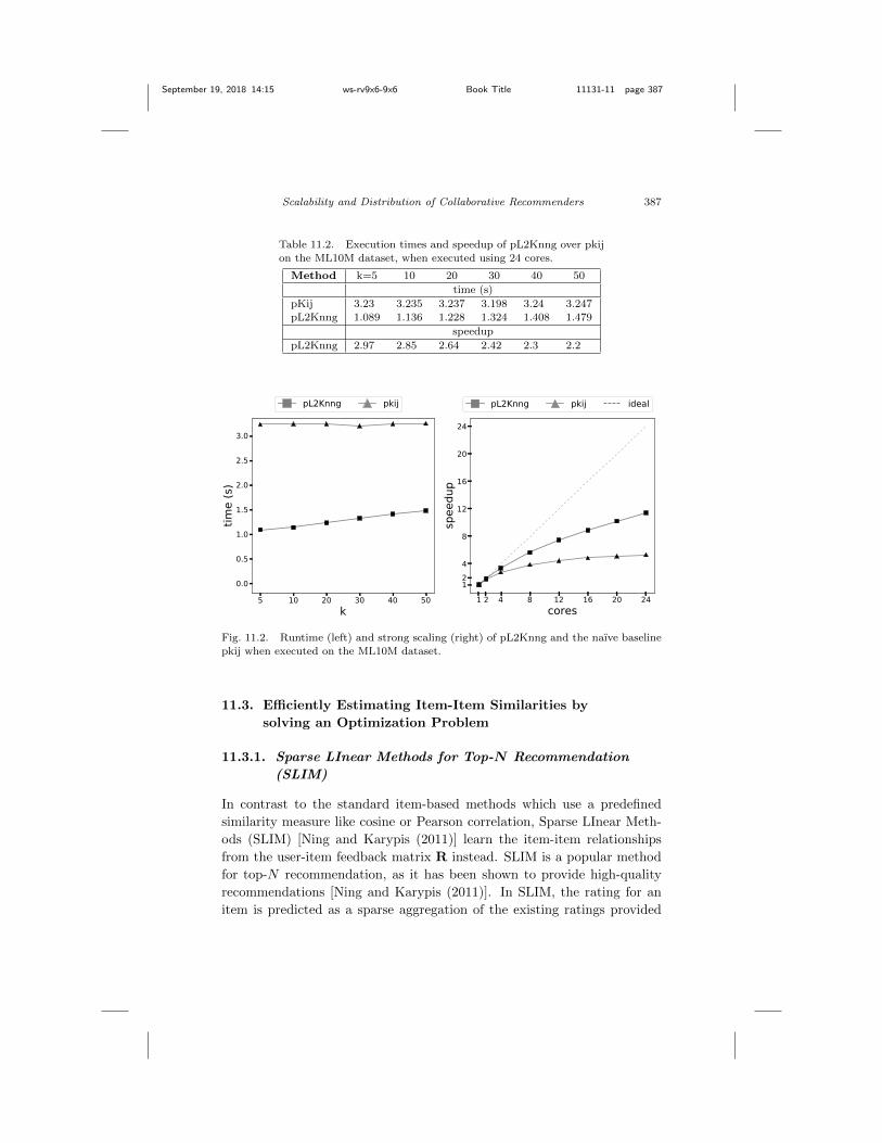
Table 11.2 and Figure 11.2 show the e�ciency of the parallel method,pL2Knng, when building the kNNG for items in the ML10M trainingdatasets, given k ranging between 5 and 50. Our method, pL2Knng, iscompared against pkij, a similar baseline to pij that uses similar cache-tiling strategies but does not prune the search space. The left graphof Figure 11.2 shows execution times in seconds, averaged over all threetraining folds, while the right one shows strong scaling results for thetwo methods, measuring the speedup of each method against their ownserial execution. By e↵ectively eliminating unnecessary similarity compu-tations, pL2Knng is able to achieve 2.2x–2.97x speedup over pkij for di↵er-ent k values. Given larger datasets, such as one containing 1M pages fromthe English Wikipedia Web site, containing almost half a billion non-zero



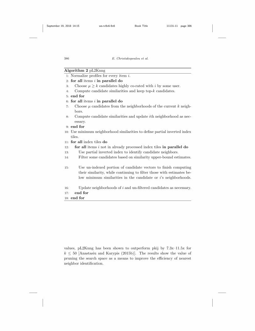
Algorithm 2 pL2Knng

1: Normalize profiles for every item i.2: for all items i in parallel do3: Choose µ � k candidates highly co-rated with i by some user.4: Compute candidate similarities and keep top-k candidates.5: end for6: for all items i in parallel do7: Choose µ candidates from the neighborhoods of the current k neigh-

bors.8: Compute candidate similarities and update ith neighborhood as nec-

essary.9: end for

10: Use minimum neighborhood similarities to define partial inverted indextiles.

11: for all index tiles do12: for all items i not in already processed index tiles in parallel do13: Use partial inverted index to identify candidate neighbors.14: Filter some candidates based on similarity upper-bound estimates.

15: Use un-indexed portion of candidate vectors to finish computingtheir similarity, while continuing to filter those with estimates be-low minimum similarities in the candidate or i’s neighborhoods.

16: Update neighborhoods of i and un-filtered candidates as necessary.17: end for18: end for

values, pL2Knng has been shown to outperform pkij by 7.3x–11.5x fork 50 [Anastasiu and Karypis (2015b)]. The results show the value ofpruning the search space as a means to improve the e�ciency of nearestneighbor identification.



Table 11.2. Execution times and speedup of pL2Knng over pkij

on the ML10M dataset, when executed using 24 cores.

Method k=5 10 20 30 40 50

time (s)

pKij 3.23 3.235 3.237 3.198 3.24 3.247

pL2Knng 1.089 1.136 1.228 1.324 1.408 1.479

speedup

pL2Knng 2.97 2.85 2.64 2.42 2.3 2.2

Fig. 11.2. Runtime (left) and strong scaling (right) of pL2Knng and the naıve baseline

pkij when executed on the ML10M dataset.

11.3. E�ciently Estimating Item-Item Similarities bysolving an Optimization Problem

11.3.1. Sparse LInear Methods for Top-N Recommendation

(SLIM)

In contrast to the standard item-based methods which use a predefinedsimilarity measure like cosine or Pearson correlation, Sparse LInear Meth-ods (SLIM) [Ning and Karypis (2011)] learn the item-item relationshipsfrom the user-item feedback matrix R instead. SLIM is a popular methodfor top-N recommendation, as it has been shown to provide high-qualityrecommendations [Ning and Karypis (2011)]. In SLIM, the rating for anitem is predicted as a sparse aggregation of the existing ratings provided



by the user:

rui = rTu si,

where rTu is the uth row of the rating matrix R and si is a sparse vec-

tor containing non-zero aggregation coe�cients over all items. The sparseaggregation coe�cient matrix S of size m ⇥ m, capturing the item-itemrelationships is estimated by solving the following optimization problem:

minimizeS

1

2||R�RS||2F +

�

2||S||2F + �||S||1

subject to S � 0

diag(S) = 0.

(11.4)

The optimization problem of Equation 11.4 tries to minimize the train-ing error, denoted by ||R � RS||2F , while also regularizing the matrix S.The problem uses two regularizers. The first one is the Frobenius norm ofthe matrix S (noted by ||S||2F ), which is controlled by the parameter �, inorder to prevent overfitting. The other regularizer is the l1 norm of thematrix S (noted by ||S||1), which is controlled by the parameter �, in orderto promote sparsity [Tibshirani (1996)]. Larger values of � and � leads tomore severe regularization. The use of both lF and l1 regularization makesthe optimization problem of Equation 11.4 an elastic net problem [Zou andHastie (2005)].

The non-negativity constraint on S imposes the item-item relations tobe positive. The constraint diag(S) = 0 is added to avoid trivial solutions(e.g., S corresponding to the identity matrix) and ensure that rui is notused to compute rui.

11.3.1.1. Parallelizing SLIM

Equation 11.4 can be accelerated by learning similarities in parallel for everytarget item i, as every column of S can be learned independently from theother columns. Then the optimization problem of Equation 11.4 changesto a set of optimization problems of the form:

minimizesi

1

2||ri �Rsi||

22 +

�

2||si||

22 + �||si||1

subject to si � 0

sii = 0,



which allows us to estimate the ith column of S, noted by si. The term ri

refers to the ith column of the training matrix R. The problem is solvedwith the use of coordinate descent and soft thresholding [Friedman et al.(2010)].

The software implementation of SLIM provided by the author Xia Ning2

utilizes the property that di↵erent columns of the sparse aggregation coef-ficient matrix can be solved independently and allows the users to specifywhich columns of the sparse aggregation coe�cient matrix they would liketo estimate. The software is implemented with the use of the Bound Con-strained Least Squares (BCLS) library3.

In order to fully utilize the benefits from the parallel estimation of dif-ferent columns of S, we use a multithreaded implementation of SLIM whichrelies on OpenMP. This allows us to have parallelism within a multi-corenode. Each thread is assigned a set of columns i and estimates the as-sociated sparse aggregation coe�cient vectors si. After all the threadshave estimated the set of si vectors, the vectors are combined into theoverall sparse aggregation coe�cient matrix S. We will refer to the mul-tithreaded implementation of SLIM, as mt-SLIM. Figure 11.3 shows thespeedup achieved by mt-SLIM on the ML10M dataset, with respect to theserial runtime (cores = 1). The results shown correspond to the time takenfor model estimation and they correspond to the average of three folds.

Fig. 11.3. The speedup achieved by mt-SLIM on the ML10M dataset, while increasing

the number of cores (strong scaling).

2http://www-users.cs.umn.edu/⇠xning/slim/html/3http://www.cs.ubc.ca/⇠mpf/bcls/index.html



As both the rating matrix and the estimated sparse aggregation coe�-cient matrix are sparse, they are stored in CSR (Compressed Sparse Row)format, in which three one-dimensional arrays are stored, that contain thenon-zero values, with their associated row and column indices.

11.3.1.2. Accelerating the training time of SLIM during parametersearch

In order to find the pair of regularization parameters � and � that give thebest results, a parameter search needs to be conducted. However, the num-ber of models to estimate increases quadratically with the number of valuesof the regularization parameters � and � explored. In order to be able toestimate the models more e�ciently, mt-SLIM utilizes ‘warm-start’. Thismeans that with the exception of the model estimated with the very firstchoice of parameters, every subsequent model is initialized with the previ-ous model estimated with a di↵erent choice of regularization parameters,instead of being initialized with zero values.

Figure 11.4 compares the time spent by mt-SLIM without initializationand mt-SLIM with warm start, for the same number of cores and and forthe same choice of regularization parameters (� = 10, � = 1). We can seethat mt-SLIM with warm start is on average 15 times faster than mt-SLIMwith no initialization.

Fig. 11.4. The time in minutes achieved by mt-SLIM with and without warm start on

the ML10M dataset for � = 10 and � = 1, while increasing the number of cores (strong

scaling).

By evaluating the performance of mt-SLIM with no initialization andwith warm start, we get the same performance results, which shows thatwith warm start, we gain in estimation times, without compromising thequality of the performance.



11.3.2. Global and Local Sparse LInear Methods for Top-NRecommendation (GLSLIM)

A limitation of SLIM is that it estimates only a single model for all theusers. In many cases, there are di↵erences in users’ behavior, who canhave diverse preferences. These cannot be captured by a single model.Recently, GLSLIM [Christakopoulou and Karypis (2016)] was proposed,which utilizes both user-subset specific models and a global model, andwas shown to improve the top-N recommendation quality. The models,(which are estimated with SLIM) are jointly optimized and combined in apersonalized way. Also, GLSLIM automatically identifies the appropriateuser subsets. If we note the global model as S and the local user-subsetspecific models as Spu , where pu 2 {1..k} denotes the user subset, thenthe predicted rating of user u, who belongs to subset pu for item i, will beestimated as:

rui =X

l2Ru

gusli + (1� gu)spu

li , (11.5)

where sli shows the global item-item similarity between the lth item ratedby the user u and the target item i and s

pu

li shows the pu user-subset specificsimilarity between the lth rated item by u and the target item i. The termgu is the personalized weight which controls the interplay between the globaland the local model and ranges between 0 and 1.

GLSLIM is an iterative algorithm which jointly optimizes the globaland local models, the user assignment and the personalized weights. Theglobal and local models are estimated by solving an elastic net optimizationproblem. Following SLIM, GLSLIM can estimate the columns of its globaland local models independent of the other columns. Separate regulariza-tion is enforced on the global and on the local models, in order to allowmore flexibility in model estimation: we thus have the global l2 regulariza-tion parameter �g, the global l1 regularization parameter �g, the local l2regularization parameter �l and the local l1 regularization parameter �l.Initially, the users are assigned to clusters. In each iteration, every useris assigned to the subset that resulted in the smallest training error, andhis personalized weight is updated accordingly. The models and the userassignment with the personalized weights are updated iteratively, until con-vergence (the algorithm converges when the users switching subsets are lessthan one percent). An overview of the algorithm is shown in Algorithm 3.



Algorithm 3 GLSLIM1: Assign gu = 0.5, to every user u.2: Compute the initial clustering of users with CLUTO4.3: while number of users who switched clusters > 1% of the total number

of users do4: Estimate S and Spu , 8pu 2 {1, . . . , k}. The estimation is initialized

in all iterations but the first one with the corresponding matrices Sand Spu , 8pu 2 {1, . . . , k} computed in the previous iteration.

5: for all user u do6: for all cluster pu do7: Compute gu for cluster pu by minimizing the squared error.8: Compute the training error.9: end for

10: Assign user u to the cluster pu that has the smallest training errorand update gu to the corresponding one for cluster pu.

11: end for12: end while

After having completed the training, the top-N recommendation is per-formed in the following way: for user u, the ratings of all the unrated items iare estimated with Equation 11.5, and the items with the N highest ratingsare recommended to the user.

11.3.2.1. Parallelizing GLSLIM

We can see from Algorithm 3 that every iteration has two parts: estimatingthe global and local models (line 4) and user refinement (lines 5�11). Bothparts allow for parallelization, each in its own way. The model estimationpart can be parallelized with respect to the items, since every column of themodels can be estimated independently of the others. The user refinementpart can be parallelized with respect to the users, as provided the modelsare fixed, the assignment and personalized weight of each user does notdepend on the other users.

Taking advantage of these parallelization opportunities, there is an MPI-based GLSLIM software5, which we use for our subsequent experiments.GLSLIM relies on MPI, instead of OpenMP which was used for mt-SLIM,as it requires more computations than SLIM. SLIM solves one elastic net4http://glaros.dtc.umn.edu/gkhome/cluto/cluto/overview5http://www-users.cs.umn.edu/⇠evangel/code.html



problem for the whole training matrix R, while GLSLIM is iterative andin each iteration, a new elastic net problem is solved for the global matrixand for all user subsets. Thus, the distributed framework MPI is employed,which allows model estimation and user refinement to be done in a dis-tributed way, thus taking advantage of multiple nodes (where each nodeconsists of cores).

Figure 11.5 shows the speedup achieved by GLSLIM on di↵erent nodes,with respect to the time taken by GLSLIM on one node (which consists of24 cores in our shown results), for the ML10M dataset.

Fig. 11.5. The speedup achieved by GLSLIM on the ML10M dataset, while increasing

the number of nodes. The speedup is computed with respect to the time of running

GLSLIM on one node.

11.3.2.2. Accelerating the training time of GLSLIM duringparameter search

GLSLIM has many parameters, for which a parameter search needs to beconducted in order to find the set of them that gives the best performance:the regularization parameters �g, �g, �l, �l, and the number of user subsetsk. We can see that the cost of finding the best possible set of parametersincreases exponentially. It is thus crucial to be able to run GLSLIM ase�ciently as possible.

In order to do so, we again employ warm start. This is done in thefollowing way: When estimating a model with a new choice of parameters,we use another model learned with a di↵erent choice of parameters as itsinitialization. Thus, the only time it is needed to estimate a model with



no initialization is when estimating the very first model for this dataset(model of the first iteration with the first choice of parameters). After it isestimated, the models of the subsequent iterations get initialized with themodels of the previous iterations. Then, when moving on to a new choiceof parameters, the model of the first iteration is initialized with the modelestimated with the previous choice of parameters and so on.

Figure 11.6 shows the time taken in minutes to run GLSLIM on ML10Mwith ‘warm start’ and with ‘no initialization’. Figure 11.6 shows the to-tal time for all iterations when run with k = 5 user subsets and with l2

regularizations parameters �g = �l = 10 and l1 regularization parameters�g = �l = 1. Note that four iterations were needed until convergence. Alsonote that the greatest part of the time shown corresponds to the modelestimations, as the user refinement does not take more than a couple ofseconds (in this example, the user refinement part took fourteen secondswhen run on one node). A speedup of 4⇥ is achieved by employing warmstart.

Fig. 11.6. The total time in minutes achieved by GLSLIM with and without warm start

on the ML10M dataset, while increasing the number of nodes.

Table 11.3 shows the top-N recommendation performance and trainingtimes of SLIM and GLSLIM with warm start, when run with the sameparameters � = �g = �l = 10 and � = �g = �l = 1. Five user sub-sets were used for GLSLIM. The top-N performance is measured in termsof HR (Equation 11.1) and ARHR (Equation 11.2). The reported timecorresponds to running SLIM and GLSLIM on one node (24 cores). Thisis done for fairness of comparison between the two methods. The showntimes correspond to the warm-start right-most column of Figure 11.4 andthe warm-start left-most column of Figure 11.6. We can see that GLSLIMhas an average performance gain of 9.5% over SLIM, while requiring more



Table 11.3. Comparison of SLIM with GLSLIM in

terms of top-N performance and training time.

Method HR ARHR Time (min)

SLIM 0.310 0.152 2.56

GLSLIM 0.336 0.167 51.72

Time corresponds to ‘warm start’ time in minutes, andcorresponds to the time taken on one node (24 cores).GLSLIM time corresponds to total time of all iterationsuntil convergence.

time-consuming training; although higher number of nodes used allows forgreat decrease in running time.

11.4. Scaling up latent factor approaches

Latent factor approaches are a class of methods that map users and items tovectors in a common low-rank space known as the latent space. A detailedoverview of latent space approaches can be found in Chapter 2. Latentfactor approaches are perhaps the most popular techniques used for ratingprediction. The success of these approaches has led to a wealth of researchon developing algorithms to facilitate high-quality recommendations frommassive training datasets. These algorithms exhibit complex tradeo↵s interms of computational characteristics, convergence rate, and available par-allelism.

11.4.1. Overview of matrix and tensor factorization

Matrix factorization approaches [Koren (2008)] are state-of-the-art collab-orative filtering methods and have gained high popularity since the NetflixPrize [Koren (2009); Takacs et al. (2009)]. They assume that the user-itemrating matrix R is low rank and can be computed as a product of twomatrices known as the user and the item latent factors (denoted P and Q,respectively). Rows of P and Q are F -dimensional vectors which representthe corresponding user or item. The value F is referred to as the rank ofthe factorization.

An item’s latent factor, denoted qi, represents a few characteristics ofthe item, and a user’s latent factor, denoted pu, signifies how much a userweights these characteristics. The predicted rating for the user u on theitem i is given by

rui = pTu qi.



The completed matrix R = PQT is used to serve the recommendationto the user for the items for which their preferences were unknown in theoriginal matrix R.

The user and the item latent factors are estimated by minimizing aregularized squared loss

minimizeP,Q

1

2

X

rui2R

�rui � pT

u qi

�2+

�

2

�||P||

2F + ||Q||

2F

�, (11.6)

where the parameter � controls the Frobenius norm regularization to pre-vent overfitting.

Additionally, instead of optimizing for rating predictions, one can op-timize for ranking performance by substituting a ranking loss function in-stead of the squared error loss function. For example, Bayesian PersonalizedRanking (BPR) [Rendle and Schmidt-Thieme (2010)], Collaborative Less-is-More Filtering (CLiMF) [Shi et al. (2012)] and CofiRank [Weimer et al.(2008)] optimize approximation of di↵erent ranking metrics to estimate theuser and the item latent factors for better ranking performance.

Ratings are often accompanied by contextual information associatedwith the ratings. For example, the ML10M dataset provides both times-tamps and tags which can be used to improve recommendation quality.

The traditional ratings matrix can be extended to include contextualinformation in the form of a tensor, which is the generalization of a matrixto higher orders. For example, associating each rating with a timestampwould result in a third-order tensor whose modes represent users, items,and time. Latent factor approaches can be extended to include higher-orderdata provided by tensors. The canonical polyadic decomposition (CPD) isa popular model for tensor factorization which has be used successfully forrating prediction. The CPD seeks to model a ratings tensor R as the com-bination of user factor P, item factor Q, and context factor C. The resultingoptimization problem closely resembles that of matrix factorization:

minimizeP,Q,C

1

2

X

ruik2R

0

@ruik �

FX

f=1

pufqifckf

1

A2

+�

2

�||P||

2F + ||Q||

2F + ||C||

2F

�.

The estimation of user and item latent factors by solving Equation 11.6 isone method of solving a problem referred to as matrix completion. It is anon-convex and computationally expensive problem. Several optimizationalgorithms have been successfully applied for matrix completion on largescale datasets.



Experimental environment. In the remaining discussion, we evaluatethree latent factor approaches that solves matrix completion problem. Eachalgorithm is iterative in nature, though by convention we refer to theseiterations as epochs. We define an epoch as the work required to updatethe latent factors one time using all available rating data. Convergenceis detected when the RMSE does not improve for twenty epochs. We fixF , the rank of the factorization, to 40. All presented results are collectedusing SPLATT [Smith and Karypis (2015)], a publicly available6 toolkit forhigh-performance sparse tensor factorizations. While optimized for tensors,SPLATT supports matrix factorizations because a matrix is equivalent toa two-mode tensor. SPLATT has also been integrated into the Spark+MPIframework [Anderson et al. (2017)], achieving over 10⇥ speedup over pureSpark solutions.

11.4.2. Alternating Least Squares (ALS)

ALS was one of the first matrix completion algorithms applied to large scaledata [Zhou et al. (2008)]. ALS is based on the observation that if we solveEquation 11.6 for one latent factor at a time, the solution has a linear leastsquares solution. ALS is an iterative algorithm which first minimizes withrespect to P and then Q. The process is repeated until convergence.

Let ru be the vector of all ratings supplied by user u. Hu is an |ru|⇥F

matrix whose rows are the feature vectors qi, for each item i rated in ru.Similarly, ri is the vector of all ratings supplied for item i, and Hi is an|ri|⇥F matrix. ALS proceeds by updating all pu followed by all qi:

pu

⇣HT

u Hu + �I⌘�1

HTu ru, 8u 2 1, . . . ,m

qi

⇣HT

i Hi + �I⌘�1

HTi ri, 8i 2 1, . . . , n.

(11.7)

The full procedure is outlined in Algorithm 4. Extending Equation 11.7to tensors changes the construction of the Hu matrices [Shao (2012)]. Forexample, the row of Hu associated with rating ruik is the elementwisemultiplication of the corresponding feature vectors qi and ck. The Hi andHk matrices are constructed similarly.

Each row in Equation 11.7 is independent and thus can be computed inparallel [Zhou et al. (2008)]. The simplicity of this approach has led ALSto be optimized for high-performance shared- and distributed-memory sys-tems[Karlsson et al. (2015); Smith et al. (2017)], GPUs [Gates et al. (2015);6http://cs.umn.edu/⇠splatt/



Algorithm 4 Matrix factorization via alternating least squares (ALS)

1: Initialize P and Q randomly.2: while P and Q have not converged do3: for all user u in parallel do4: Hu 0.5: For each rating rui in ru, append row qi to Hu.

6: pu

⇣HT

u Hu + �I⌘�1

HTu ru.

7: end for8: for all item i in parallel do9: Hi 0.

10: For each rating rui in ri, append row pu to Hi.

11: qi

⇣HT

i Hi + �I⌘�1

HTi ri.

12: end for13: end while

Tan et al. (2016)], Hadoop [Shin and Kang (2014)], and is implemented inSpark’s MLlib7. Successful approaches distribute the ratings data in a one-dimensional fashion such that all of the ratings required to construct anH matrix are located on the same node. By distributing the data in thisfashion, none of the partially-constructed H matrices need to be commu-nicated or aggregated. However, this distribution requires that each nodestores potentially the entire latent factors. Fortunately, in practice this isnot prohibitive on most modern systems.

The computational complexity of ALS is O�F

2|R|+ F

3(m+ n)�per

epoch. In practice, the O(F 2) computation per rating that comes from con-structing the various H matrices dominates the computation. A commonimplementation strategy is to process one rating at a time and accumulatedirectly into HT

u Hu and Huru instead of explicitly constructing Hu. How-ever, this strategy ignores the details of modern hardware architectures inwhich memory movement is more expensive than floating-point operations.Each rating produces an accumulation that is a rank-1 update performingO(F 2) work on F

2 data. Alternatively, performing a single rank-k updateby explicitly forming Hu instead performs O(|ru|F

2) work on (|ru|F +F2)

data [Gates et al. (2015); Smith et al. (2017)]. While the final amount ofwork is the same, the rank-k update fetches less data from memory andis thus better suited for modern processors. We explore this phenomenon

7https://spark.apache.org/mllib/



(a) Matrix (b) Tensor

Fig. 11.7. Average time per epoch when using rank-1 and rank-k updates during ALS.

Execution is on 24 cores and an epoch is counted as updating each factor matrix once.

in Figure 11.7, which illustrates runtime per epoch as F is increased. Us-ing rank-k updates can be over 10⇥ faster than the more common rank-1updates.

11.4.3. Stochastic Gradient Descent (SGD)

SGD is an optimization algorithm that trades a large number of epochs fora low computational complexity. An epoch consists of processing all ratingsone-at-a-time in random order and updating the factorization based on thelocal gradient. Updates are of the form:

eui rui � pTu qi,

pu pu + ⌘ (euiqi � �pu) ,

qi qi + ⌘ (euipu � �qi) ,

(11.8)

where ⌘ is a hyperparameter representing the learning rate. The complexityof Equation 11.8 is linear in F , resulting in a total complexity of O(F |R|)per epoch. The low complexity and simple implementation of SGD has ledto it being widely adopted by researchers and industry alike. The detailsof SGD are outlined in Algorithm 5.

SGD is less straightforward than ALS to parallelize. Since processinga rating updates rows of both P and Q, special care must be taken toprevent the same rows from being modified at the same time (called a racecondition). There are two broad approaches for parallelizing SGD.

Stratified methods are based on the observation that if two ratings donot overlap (i.e., they have neither a row nor a column in common) thenthey can be updated with Equation 11.8 in parallel. This strategy was



Algorithm 5 Matrix factorization via stochastic gradient descent (SGD)

1: Initialize P and Q randomly.2: while P and Q have not converged do3: Shu✏e the permutation of ratings.4: for all rating rui do5: eui rui � pT

u qi

6: pu pu + ⌘ (euiqi � �pu).7: qi qi + ⌘ (euipu � �qi).8: end for9: end while

P

QT

P

QT

P

QT

(a) (b) (c)

Fig. 11.8. Stratified SGD with three workers. Colored blocks represent independent

sets of ratings and the rows of P and Q which model them. Each colored block of

ratings and their corresponding rows can be processed in parallel.

introduced by DSGD [Gemulla et al. (2011)], which imposes a grid on Rto identify blocks that can be processed in parallel. Stratification is illus-trated in Figure 11.8. Stratification has proven to be an e↵ective strategyfor parallelizing SGD and has been extended in works on multithreadedenvironments, distributed systems, and GPUs [Zhuang et al. (2013); Yunet al. (2014); Xie et al. (2017)].

Asynchronous methods rely on the stochastic nature of SGD to allowoverlapping updates. This technique was popularized by Hogwild [Rechtet al. (2011)] on shared-memory systems. The key idea is to simply allowrace conditions to occur without attempting to avoid them. Convergenceis still achieved due to the iterative nature of SGD and infrequent overlapsfrom the high level of sparsity in R. Teflioudi et al. later introduced asyn-chronous SGD (ASGD) [Teflioudi et al. (2012)] for distributed computingenvironments. During ASGD, nodes maintain locally modified copies of P



and Q and updates are asynchronously communicated several times perepoch. Overlapping updates are averaged with the master copy and sentto workers.

Extending the formulation of SGD to tensors is straightforward andagain only requires additional elementwise multiplications [Shao (2012)].However, parallelization becomes a significant challenge when a contextualmode is added to the data. The number of blocks in a stratified SGD al-gorithm increases exponentially with the number of tensor modes despitethe work per rating only increasing linearly, and thus the time of syn-chronization and communication quickly dominate the factorization time.Asynchronous methods also su↵er because the number of unique contextsis typically much smaller than the number of users or items, resulting inmore frequent update conflicts. A hybrid of stratification and asynchronousSGD addresses these challenges, but the hybrid is still bested by ALS atlarge numbers of cores [Smith et al. (2017)].

11.4.4. Coordinate Descent (CCD++)

Coordinate descent is a class of optimization algorithms which update oneparameter of the output at a time. CCD++ is a column-oriented de-scent algorithms for matrix completion [Yu et al. (2012)]. CCD++ updatescolumns of P and Q in sequence, with a single parameter update takingthe form

puf

Prui2R(rui � pT

u qi + pufqif )qif

� +P

rui2R q2if

. (11.9)

The full procedure is outlined in Algorithm 4. If all (rui � pTu qi) are

pre-computed, CCD++ has a complexity of O(F |R|) per epoch, match-ing SGD. The extension of CCD++ to tensors follows that of ALS andSGD, in which additional elementwise multiplications are introduced tothe formulation [Karlsson et al. (2015)].

Similar to ALS, each column entry is independent and can thus becomputed in parallel. CCD++ has accordingly been parallelized on shared-and distributed-memory systems [Yu et al. (2012); Karlsson et al. (2015);Smith et al. (2017)] and GPUs [Nisa et al. (2017)]. However, unlike ALS,the communication cost from aggregating partial computations is only ofconstant size per column as opposed to the larger H matrices of ALS.The lower communication volume a↵ords more flexible partitionings of theratings. Recent work has shown that a Cartesian (i.e., grid) distribution



Algorithm 6 Matrix factorization via coordinate descent (CCD++)

1: Initialize P and Q randomly.2: while P and Q have not converged do3: for all column f do4: Pre-compute all error terms: (rui � pT

u qi).5: for all user u in parallel do6: Update puf following (11.9).7: end for8: for all item i in parallel do9: Update qif following (11.9).

10: end for11: end for12: end while

of the data is an e↵ective formulation and has been scaled to over sixteenthousand cores [Smith et al. (2017)].

11.4.5. Evaluation of optimization algorithms

Parallel scalability. We examine the parallel scalability of ALS, SGD,and CCD++ for matrix and tensor completion in Figure 11.9. ALS scalesnotably better than the competing methods. The scalability of ALS comesfrom being rich in dense linear algebra kernels which e↵ectively use thefloating-point hardware found in each core, instead of being bound by mem-ory bandwidth which is a shared resource. In contrast, SGD and CCD++perform a factor of F fewer floating-point operations per rating processed,resulting in heavy reliance on available memory bandwidth. Interestingly,the scalability of CCD++ and SGD is also more dependent on the size andcharacteristics of the ratings dataset. Figure 11.10 shows parallel scalabil-ity on a tensor of 210 million Yahoo! music ratings with timestamps fromthe 2011 KDD cup [Dror et al. (2012)]. CCD++ achieves perfect speedupon this significantly larger and more sparse dataset.

Time to solution. Finally, we compare solution qualities and conver-gence times for the latent factor approaches in Table 11.4. In the matrixcase, SGD arrives at the lowest RMSE while being competitive in runtimeto ALS. CCD++ obtains the lowest RMSE in the tensor case, but at 5⇥ theruntime of the similar-quality ALS. Utilizing the timestamp for tensor com-pletion notably improves the RMSE for ALS and CCD++, but not SGD.



(a) Matrix (b) Tensor

Fig. 11.9. Speedup on ML10M dataset scaling from 1 to 24 cores. SGD is parallelized

using Hogwild [Recht et al. (2011)].

Fig. 11.10. Parallel speedup on a three-mode tensor made from 210 million Yahoo!

music ratings.

Since timestamps are grouped by month (133 months in total), the numberof independent months is significantly more limited than the number of in-dependent users or items. Thus, there are frequent overlapping updates tothe C latent factor. Lastly, we note that the time-to-solution for CCD++is longer in the matrix case than the tensor case, despite performing lesswork and arriving at a higher RMSE. While the tensor completion algo-rithm performs more work than the matrix equivalent, in practice we findthat it converges in fewer epochs.



Table 11.4. Comparison of solution quality and time.

Matrix TensorAlgorithm RMSE Time (s) RMSE Time (s)ALS 0.8805 4.82 0.8662 50.26

SGD 0.8747 11.54 0.9107 17.19

CCD++ 0.8955 435.61 0.8622 256.25

RMSE is evaluated on the test dataset, averaged over three folds.Time measures the time to convergence.

11.4.6. Singular Value Decomposition (SVD)

The key idea of SVD-based models is to factorize the user-item rating ma-trix to a product of two lower rank matrices, one containing the user factorsand the other containing the item factors. Since conventional SVD is unde-fined in the presence of missing values, PureSVD [Cremonesi et al. (2010)]treats all the missing values as zeros prior to the application of the standardSVD method. PureSVD is shown to be suitable for the top-N recommen-dations task. The better top-N recommendation performance of PureSVDin comparison to the standard matrix completion-based approaches thatare optimized for rating predictions, can be attributed to the fact that itconsiders all the items present in the catalog rather than considering onlythe items rated by the user. Additionally, for ranking purposes, it doesnot need to predict the exact ratings but only requires to achieve a correctrelative ordering of the predictions for a user.

PureSVD estimates the rating matrix R as

R = U⌃QT,

where U is a n⇥F orthonormal matrix, Q is an m⇥F orthonormal matrixand ⌃ is an F ⇥ F diagonal matrix, containing the F largest singularvalues. It can be noted that the matrix P representing the user factors canbe derived by

P = U⌃.

The matrices U, ⌃ and Q can be estimated by solving the following opti-mization problem with orthonormal constraints

minimizeU,Q,⌃

1

2||R�

FX

i=1

�iuiqTi ||

2F

subject to UT U = I

QT Q = I,

(11.10)



where I is the identity matrix, �i denotes the ith largest singular value,ui represents the ith column vector of U and qi denotes the ith columnvector of Q. The application of PureSVD on large scale sparse matricescan be optimized with the Golub-Kahan-Lanczos Bidiagonalization [Goluband Kahan (1965); Lanczos (1950)] approach. It computes the SVD of givenmatrix R in two steps. First, it bidiagonalizes R using Lanczos procedureas,

R = PBQT, (11.11)

where P and Q are unitary matrices, and B is an upper bidiagonal matrix.The Lanczos procedure can take advantage of optimized sparse matrix-vector multiplications and e�cient orthogonalization. Then, it uses ane�cient method [Demmel and Kahan (1990)] to compute the singular valuesof B without computing BT B as,

B = X⌃YT. (11.12)

Now, using Equations 11.11 and 11.12 we can compute left singular vectors,i.e., U = PX, and right singular vectors, i.e., V = QY, of matrix R.

Modern randomized matrix approximation techniques [Halko et al.(2011)] can be used to compute a faster but approximate SVD of the ratingmatrix. We will refer to these approximation techniques as RandomizedSVD. Essentially, Randomized SVD technique is carried out in two steps.First, it tries to find Q with F orthonormal columns such that,

R ⇡ QQT A. (11.13)

Next, it constructs B = QT A, and since B has relatively smaller numberof rows, i.e., F , we can employ standard methods to e�ciently computeSVD of B as,

B = U⌃VT. (11.14)

Thus, left singular vector of R can be approximated by, U = QU, andright singular vectors can be approximated by V. Randomized SVD cantake advantage of e�cient sparse matrix-matrix multiplication to find Qand to compute B.

For our experiments, we used the optimized and parallel implementationof Golub-Kahan-Lanczos Bidiagonalization approach available in SLEPc8

[Hernandez et al. (2007)] for PureSVD, and utilized the implementationof Randomized SVD available in RedSVD9. These implementations rely8slepc.upv.es

9https://github.com/ntessore/redsvd-h



Fig. 11.11. Speedup (left) and total time in seconds (right) achieved by PureSVD and

Randomized SVD on the ML10M dataset (F = 500).

on well-studied sparse and dense linear algebra operations, that are fur-ther optimized for e�cient usage on high-performance computers [Ander-son et al. (1990)]. Figure 11.11 shows the speedup and total time achievedby PureSVD and Randomized SVD on ML10M dataset with increasingnumber of cores. As can be seen in the figure, the parallel implementationof PureSVD achieves better speedup than Randomized SVD with increasein the number of cores. Also, the time taken by Randomized SVD is lowerin comparison to that of PureSVD on a single core. Table 11.5 presentsthe results for the best ranking performance achieved by both the methodson ML10M dataset. As can be seen in the table, PureSVD and Random-ized SVD do not outperform SLIM for top-N recommendation but thetime taken by PureSVD and Randomized SVD is lower than that of SLIM.Furthermore, PureSVD outperforms Randomized SVD for top-N recom-mendation performance. We should note though that the performance ofRandomized SVD is comparable to that of PureSVD, and therefore Ran-domized SVD can serve as an alternative to PureSVD under time andcompute resource constraints. Also, Randomized SVD needs higher rankto achieve its best performance.

11.5. Conclusion

In this chapter, we presented di↵erent methods which speed up popularcollaborative recommenders, by taking advantage of modern parallel multi-core architectures. We discussed ways to e�ciently identify neighbors in



Table 11.5. Comparison of PureSVD with Randomized SVD in

terms of top-N performance and training time.

Method HR ARHR Rank (F ) Time (sec)

PureSVD 0.292 0.139 60 9.24

Randomized SVD 0.247 0.112 400 15.46

Time corresponds to the time taken on one node (24 cores).

k-nearest neighbor approaches in Section 11.2. We investigated how toparallelize the sparse linear methods well-suited for the top-N recommen-dation task, presented in Section 11.3 and how to speed up their parametersearch. Finally, in Section 11.4, we showed ways to scale up the latent fac-tor approaches, which could extend to tensor factorization approaches. Ineach section, we also presented experimental results on the popular ML10Mdataset, illustrating the runtimes and speedup achieved in comparison toserial core implementations. Overall, the goal of this chapter is to illustratethat modern popular collaborative recommenders, although of very di↵er-ent nature, are able to be parallelized. We believe that research that focuseson ways to distribute and scale popular collaborative recommenders is cru-cial, as it leads to faster training times without sacrificing recommendationquality.

References

Anastasiu, D. C. (2017). Cosine approximate nearest neighbors, in P. Haber,T. Lampoltshammer and M. Mayr (eds.), Data Science – Analytics andApplications, iDSC 2017 (Springer Fachmedien Wiesbaden, Wiesbaden),ISBN 978-3-658-19287-7, pp. 45–50.

Anastasiu, D. C. and Karypis, G. (2014). L2ap: Fast cosine similarity search withprefix l-2 norm bounds, in 30th IEEE International Conference on DataEngineering, ICDE ’14, pp. 784–795, doi:10.1109/ICDE.2014.6816700.

Anastasiu, D. C. and Karypis, G. (2015a). L2knng: Fast exact k-nearest neigh-bor graph construction with l2-norm pruning, in 24th ACM Interna-tional Conference on Information and Knowledge Management, CIKM ’15(ACM, New York, NY, USA), ISBN 978-1-4503-3794-6, pp. 791–800, doi:10.1145/2806416.2806534, http://doi.acm.org/10.1145/2806416.2806534.

Anastasiu, D. C. and Karypis, G. (2015b). Pl2ap: Fast parallel cosine similaritysearch, in Proceedings of the 5th Workshop on Irregular Applications: Archi-tectures and Algorithms, IA3 ’15 (ACM, New York, NY, USA), pp. 8:1–8:8.

Anastasiu, D. C. and Karypis, G. (2016). Fast parallel cosine k-nearest neigh-bor graph construction, in 2016 6th Workshop on Irregular Applications:Architecture and Algorithms (IA3), pp. 50–53, doi:10.1109/IA3.2016.013.



Anderson, E., Bai, Z., Dongarra, J., Greenbaum, A., McKenney, A., Du Croz, J.,Hammarling, S., Demmel, J., Bischof, C. and Sorensen, D. (1990). Lapack:A portable linear algebra library for high-performance computers, in Pro-ceedings of the 1990 ACM/IEEE Conference on Supercomputing, Supercom-puting ’90 (IEEE Computer Society Press, Los Alamitos, CA, USA), ISBN0-89791-412-0, pp. 2–11, http://dl.acm.org/citation.cfm?id=110382.110385.

Anderson, M., Smith, S., Sundaram, N., Capota, M., Zhao, Z., Dulloor, S., Satish,N. and Willke, T. L. (2017). Bridging the gap between HPC and Big Dataframeworks, Proceedings of the VLDB Endowment (PVLDB ’17).

Bayardo, R. J., Ma, Y. and Srikant, R. (2007). Scaling up all pairs similaritysearch, in Proceedings of the 16th International Conference on World WideWeb, WWW ’07 (ACM, New York, NY, USA), pp. 131–140.

Christakopoulou, E. and Karypis, G. (2016). Local item-item models for top-nrecommendation, in Proceedings of the 10th ACM Conference on Recom-mender Systems (ACM), pp. 67–74.

Cremonesi, P., Koren, Y. and Turrin, R. (2010). Performance of recommender al-gorithms on top-n recommendation tasks, in Proceedings of the Fourth ACMConference on Recommender Systems, RecSys ’10 (ACM, New York, NY,USA), ISBN 978-1-60558-906-0, pp. 39–46, doi:10.1145/1864708.1864721,http://doi.acm.org/10.1145/1864708.1864721.

Demmel, J. and Kahan, W. (1990). Accurate singular values of bidiagonal matri-ces, SIAM Journal on Scientific and Statistical Computing 11, 5, pp. 873–912.

Deshpande, M. and Karypis, G. (2004). Item-based top-n recommendation algo-rithms, ACM Transactions on Information Systems (TOIS) 22, 1, pp. 143–177.

Dror, G., Koenigstein, N., Koren, Y. and Weimer, M. (2012). The yahoo! musicdataset and kdd-cup’11. in KDD Cup, pp. 8–18.

Friedman, J., Hastie, T. and Tibshirani, R. (2010). Regularization paths for gen-eralized linear models via coordinate descent, Journal of statistical software33, 1, p. 1.

Gates, M., Anzt, H., Kurzak, J. and Dongarra, J. (2015). Accelerating collabora-tive filtering using concepts from high performance computing, in Big Data(Big Data), 2015 IEEE International Conference on (IEEE), pp. 667–676.

Gemulla, R., Nijkamp, E., Haas, P. J. and Sismanis, Y. (2011). Large-scale matrixfactorization with distributed stochastic gradient descent, in Proceedings ofthe 17th ACM SIGKDD international conference on Knowledge discoveryand data mining (ACM), pp. 69–77.

Golub, G. and Kahan, W. (1965). Calculating the singular values and pseudo-inverse of a matrix, Journal of the Society for Industrial and Applied Math-ematics, Series B: Numerical Analysis 2, 2, pp. 205–224.

Halko, N., Martinsson, P.-G. and Tropp, J. A. (2011). Finding structure withrandomness: Probabilistic algorithms for constructing approximate matrixdecompositions, SIAM review 53, 2, pp. 217–288.

Harper, F. M. and Konstan, J. A. (2015). The movielens datasets: History andcontext, ACM Trans. Interact. Intell. Syst. 5, 4, pp. 19:1–19:19.



Hernandez, V., Roman, J., Tomas, A. and Vidal, V. (2007). Restarted lanczosbidiagonalization for the svd in slepc, STR-8, Tech. Rep.

Karlsson, L., Kressner, D. and Uschmajew, A. (2015). Parallel algorithms fortensor completion in the cp format, Parallel Computing.

Konstan, J. A., Miller, B. N., Maltz, D., Herlocker, J. L., Gordon, L. R. andRiedl, J. (1997). Grouplens: Applying collaborative filtering to usenet news,Commun. ACM 40, 3, pp. 77–87, doi:10.1145/245108.245126, http://doi.acm.org/10.1145/245108.245126.

Koren, Y. (2008). Factorization meets the neighborhood: a multifaceted col-laborative filtering model, in Proceedings of the 14th ACM SIGKDD in-ternational conference on Knowledge discovery and data mining (ACM),pp. 426–434.

Koren, Y. (2009). The bellkor solution to the netflix grand prize, Netflix prizedocumentation 81, pp. 1–10.

Lanczos, C. (1950). An iteration method for the solution of the eigenvalue problemof linear di↵erential and integral operators (United States Governm. PressO�ce Los Angeles, CA).

Ning, X. and Karypis, G. (2011). Slim: Sparse linear methods for top-n rec-ommender systems, in 2011 IEEE 11th International Conference on DataMining (IEEE), pp. 497–506.

Nisa, I., Sukumaran-Rajam, A., Kunchum, R. and Sadayappan, P. (2017). Paral-lel CCD++ on GPU for matrix factorization, in Proceedings of the GeneralPurpose GPUs (GPGPU) (ACM), pp. 73–83.

Recht, B., Re, C., Wright, S. and Niu, F. (2011). Hogwild: A lock-free approach toparallelizing stochastic gradient descent, in Advances in Neural InformationProcessing Systems, pp. 693–701.

Rendle, S. and Schmidt-Thieme, L. (2010). Pairwise interaction tensor factoriza-tion for personalized tag recommendation, in Proceedings of the third ACMinternational conference on Web search and data mining (ACM), pp. 81–90.

Sarwar, B., Karypis, G., Konstan, J. and Riedl, J. (2001). Item-based collabora-tive filtering recommendation algorithms, in Proceedings of the 10th inter-national conference on World Wide Web (ACM), pp. 285–295.

Shao, W. (2012). Tensor Completion, Master’s thesis, Universitat des SaarlandesSaarbrucken.

Shi, Y., Karatzoglou, A., Baltrunas, L., Larson, M., Oliver, N. and Hanjalic,A. (2012). Climf: learning to maximize reciprocal rank with collaborativeless-is-more filtering, in Proceedings of the sixth ACM conference on Rec-ommender systems (ACM), pp. 139–146.

Shin, K. and Kang, U. (2014). Distributed methods for high-dimensional andlarge-scale tensor factorization, in Data Mining (ICDM), 2014 IEEE Inter-national Conference on, pp. 989–994.

Smith, S. and Karypis, G. (2015). SPLATT: the Surprisingly Parallel spArseTensor Toolkit, http://cs.umn.edu/⇠splatt/.

Smith, S., Park, J. and Karypis, G. (2017). Hpc formulations of optimizationalgorithms for tensor completion, Parallel Computing.



Takacs, G., Pilaszy, I., Nemeth, B. and Tikk, D. (2009). Scalable collaborativefiltering approaches for large recommender systems, Journal of machinelearning research 10, Mar, pp. 623–656.

Tan, W., Cao, L. and Fong, L. (2016). Faster and cheaper: Parallelizing large-scale matrix factorization on gpus, in Proceedings of the 25th ACM Inter-national Symposium on High-Performance Parallel and Distributed Com-puting (ACM), pp. 219–230.

Teflioudi, C., Makari, F. and Gemulla, R. (2012). Distributed matrix comple-tion, in Data Mining (ICDM), 2012 IEEE 12th International Conferenceon (IEEE), pp. 655–664.

Tibshirani, R. (1996). Regression shrinkage and selection via the lasso, Journalof the Royal Statistical Society. Series B (Methodological), pp. 267–288.

Weimer, M., Karatzoglou, A., Le, Q. V. and Smola, A. J. (2008). Cofi rank-maximum margin matrix factorization for collaborative ranking, in Ad-vances in neural information processing systems, pp. 1593–1600.

Xie, X., Tan, W., Fong, L. L. and Liang, Y. (2017). CuMF SGD: Parallelizedstochastic gradient descent for matrix factorization on gpus, in Proceedingsof the 26th International Symposium on High-Performance Parallel andDistributed Computing (HPDC), pp. 79–92.

Yu, H.-F., Hsieh, C.-J., Dhillon, I. et al. (2012). Scalable coordinate descent ap-proaches to parallel matrix factorization for recommender systems, in DataMining (ICDM), 2012 IEEE 12th International Conference on (IEEE),pp. 765–774.

Yun, H., Yu, H.-F., Hsieh, C.-J., Vishwanathan, S. V. N. and Dhillon, I.(2014). Nomad: Non-locking, stochastic multi-machine algorithm for asyn-chronous and decentralized matrix completion, Proc. VLDB Endow. 7, 11,pp. 975–986, doi:10.14778/2732967.2732973, http://dx.doi.org/10.14778/2732967.2732973.

Zhou, Y., Wilkinson, D., Schreiber, R. and Pan, R. (2008). Large-scale parallelcollaborative filtering for the netflix prize, in Algorithmic Aspects in Infor-mation and Management (Springer), pp. 337–348.

Zhuang, Y., Chin, W.-S., Juan, Y.-C. and Lin, C.-J. (2013). A fast parallel sgdfor matrix factorization in shared memory systems, in Proceedings of the7th ACM conference on Recommender systems (ACM), pp. 249–256.

Zou, H. and Hastie, T. (2005). Regularization and variable selection via the elasticnet, Journal of the Royal Statistical Society: Series B (Statistical Method-ology) 67, 2, pp. 301–320.


Index

✏ nearest neighbor graph(✏NNG), 381

k nearest neighbor graph(kNNG), 384

all-pairs similarity search, 381alternating least squares (ALS),

397average reciprocal hit rank

(ARHR), 378, 394, 395, 407

canonical polyadicdecomposition, 396

coordinate descent (CCD++),401

distributed memory, 392, 397,400, 401

hit rate (HR), 378, 394, 395, 407

latent space approaches, 395

matrix factorization, 395

nearest-neighbor approaches, 379

parallel architectures, 376

parallel computing, 376pL2AP, 382pL2Knng, 385PureSVD, 404

rating prediction, 377, 395root mean squared error(RMSE), 379, 403

shared memory, 385, 389, 397,400, 401

similarity join, 381singular value decomposition(SVD), 404randomized, 405

sparse linear methods (SLIM),387global and local (GLSLIM),

391stochastic gradient descent(SGD), 399

strong scaling, 383, 385, 389, 390

tensor factorization, 395top-N recommendation, 377,387, 391, 404

warm start, 390, 394

411

chapter 11 scalability and distribution of collaborative …chri2951/chapter11.pdf ·...

Documents