chapter 13. modeling species transport and finite-rate ... · pdf filechapter 13. modeling...

Chapter 13. Modeling Species

Transport and Finite-Rate Chemistry

FLUENT can model the mixing and transport of chemical species by solv-ing conservation equations describing convection, diffusion, and reactionsources for each component species. Multiple simultaneous chemical re-actions can be modeled, with reactions occurring in the bulk phase (vol-umetric reactions) and/or on wall or particle surfaces. Species transportmodeling capabilities, both with and without reactions, and the inputsyou provide when using the model are described in this chapter.

Note that you may also want to consider modeling your reacting sys-tem using the mixture fraction approach (for non-premixed systems,described in Chapter 14), the reaction progress variable approach (forpremixed systems, described in Chapter 15), or the partially premixedapproach (described in Chapter 16). See Chapter 12 for an overview ofthe reaction modeling approaches available in FLUENT.

Information is divided into the following sections:

• Section 13.1: Volumetric Reactions

• Section 13.2: Wall Surface Reactions and Chemical Vapor Deposi-tion

• Section 13.3: Particle Surface Reactions

• Section 13.4: Species Transport Without Reactions

c© Fluent Inc. November 28, 2001 13-1

Modeling Species Transport and Finite-Rate Chemistry

13.1 Volumetric Reactions

Information about species transport and finite-rate chemistry as relatedto volumetric reactions is presented in the following subsections:

• Section 13.1.1: Theory

• Section 13.1.2: Overview of User Inputs for Modeling Species Trans-port and Reactions

• Section 13.1.3: Enabling Species Transport and Reactions andChoosing the Mixture Material

• Section 13.1.4: Defining Properties for the Mixture and Its Con-stituent Species

• Section 13.1.5: Defining Boundary Conditions for Species

• Section 13.1.6: Defining Other Sources of Chemical Species

• Section 13.1.7: Solution Procedures for Chemical Mixing and Finite-Rate Chemistry

• Section 13.1.8: Postprocessing for Species Calculations

• Section 13.1.9: Importing a Chemical Mechanism from CHEMKIN

13.1.1 Theory

Species Transport Equations

When you choose to solve conservation equations for chemical species,FLUENT predicts the local mass fraction of each species, Yi, throughthe solution of a convection-diffusion equation for the ith species. Thisconservation equation takes the following general form:

∂

∂t(ρYi) + ∇ · (ρ~vYi) = −∇ · ~Ji +Ri + Si (13.1-1)

where Ri is the net rate of production by chemical reaction (describedlater in this section) and Si is the rate of creation by addition from the

13-2 c© Fluent Inc. November 28, 2001


dispersed phase plus any user-defined sources. An equation of this formwill be solved for N − 1 species where N is the total number of fluidphase chemical species present in the system. Since the mass fractionof the species must sum to unity, the Nth mass fraction is determinedas one minus the sum of the N − 1 solved mass fractions. To minimizenumerical error, the Nth species should be selected as that species withthe overall largest mass fraction, such as N2 when the oxidizer is air.

Mass Diffusion in Laminar Flows

In Equation 13.1-1, ~Ji is the diffusion flux of species i, which arisesdue to concentration gradients. By default, FLUENT uses the diluteapproximation, under which the diffusion flux can be written as

~Ji = −ρDi,m∇Yi (13.1-2)

Here Di,m is the diffusion coefficient for species i in the mixture.

For certain laminar flows, the dilute approximation may not be accept-able, and full multicomponent diffusion is required. In such cases, theMaxwell-Stefan equations can be solved; see Section 7.7.2 for details.

Mass Diffusion in Turbulent Flows

In turbulent flows, FLUENT computes the mass diffusion in the followingform:

~Ji = −(ρDi,m +

µt

Sct

)∇Yi (13.1-3)

where Sct is the turbulent Schmidt number, µt

ρDt(with a default setting

of 0.7). Note that turbulent diffusion generally overwhelms laminar dif-fusion, and the specification of detailed laminar diffusion properties inturbulent flows is not warranted.



Treatment of Species Transport in the Energy Equation

For many multicomponent mixing flows, the transport of enthalpy dueto species diffusion

∇ ·[

n∑i=1

hi~Ji

]

can have a significant effect on the enthalpy field and should not beneglected. In particular, when the Lewis number

Lei =k

ρcpDi,m(13.1-4)

for any species is far from unity, neglecting this term can lead to sig-nificant errors. FLUENT will include this term by default. In Equa-tion 13.1-4, k is the thermal conductivity.

Diffusion at Inlets

For the segregated solver in FLUENT, the net transport of species atinlets consists of both the convection and diffusion components. (Forthe coupled solvers, only the convection component is included.) Theconvection component is fixed by the inlet species concentration specifiedby you. The diffusion component, however, depends on the gradient ofthe computed species concentration field. Thus the diffusion component(and therefore the net inlet transport) is not specified a priori. SeeSection 13.1.5 for information about specifying the net inlet transport ofspecies.

The Generalized Finite-Rate Formulation for Reaction Modeling

The reaction rates that appear as source terms in Equation 13.1-1 arecomputed in FLUENT by one of three models:

• Laminar finite-rate model: The effect of turbulent fluctuations areignored, and reaction rates are determined by Arrhenius expres-sions.



• Eddy-dissipation model: Reaction rates are assumed to be con-trolled by the turbulence, so expensive Arrhenius chemical kineticcalculations can be avoided.

• Eddy-dissipation-concept (EDC) model: Detailed Arrhenius chem-ical kinetics can be incorporated in turbulent flames. Note thatdetailed chemical kinetic calculations are computationally expen-sive.

The generalized finite-rate formulation is suitable for a wide range of ap-plications including laminar or turbulent reaction systems, and combus-tion systems with premixed, non-premixed, or partially-premixed flames.

The Laminar Finite-Rate Model

The laminar finite-rate model computes the chemical source terms usingArrhenius expressions, and ignores the effects of turbulent fluctuations.The model is exact for laminar flames, but is generally inaccurate forturbulent flames due to highly non-linear Arrhenius chemical kinetics.The laminar model may, however, be acceptable for combustion withrelatively slow chemistry and small turbulent fluctuations, such as su-personic flames.

The net source of chemical species i due to reaction Ri is computed asthe sum of the Arrhenius reaction sources over the NR reactions that thespecies participate in:

Ri = Mw,i

NR∑r=1

Ri,r (13.1-5)

where Mw,i is the molecular weight of species i and Ri,r is the Arrheniusmolar rate of creation/destruction of species i in reaction r. Reactionmay occur in the continuous phase between continuous-phase speciesonly, or at wall surfaces resulting in the surface deposition or evolutionof a continuous-phase species.

Consider the rth reaction written in general form as follows:



N∑i=1

ν ′i,rMi

kf,r⇀↽kb,r

N∑i=1

ν ′′i,rMi (13.1-6)

whereN = number of chemical species in the systemν ′i,r = stoichiometric coefficient for reactant i in reaction r

ν ′′i,r = stoichiometric coefficient for product i in reaction r

Mi = symbol denoting species ikf,r = forward rate constant for reaction rkb,r = backward rate constant for reaction r

Equation 13.1-6 is valid for both reversible and non-reversible reactions.(Reactions in FLUENT are non-reversible by default.) For non-reversiblereactions, the backward rate constant, kb,r, is simply omitted.

The summations in Equation 13.1-6 are for all chemical species in thesystem, but only species that appear as reactants or products will havenon-zero stoichiometric coefficients. Hence, species that are not involvedwill drop out of the equation.

The molar rate of creation/destruction of species i in reaction r (Ri,r inEquation 13.1-5) is given by

Ri,r = Γ(ν ′′i,r − ν ′i,r

)kf,r

Nr∏j=1

[Cj,r]η′

j,r − kb,r

Nr∏j=1

[Cj,r]η′′

j,r

(13.1-7)

whereNr = number of chemical species in reaction rCj,r = molar concentration of each reactant and product

species j in reaction r (kgmol/m3)η′j,r = forward rate exponent for each reactant and product

species j in reaction rη′′j,r = backward rate exponent for each reactant and product

species j in reaction r



See Section 13.1.4 for information about inputting the stoichiometriccoefficients and rate exponents for both global forward (non-reversible)reactions and elementary (reversible) reactions.

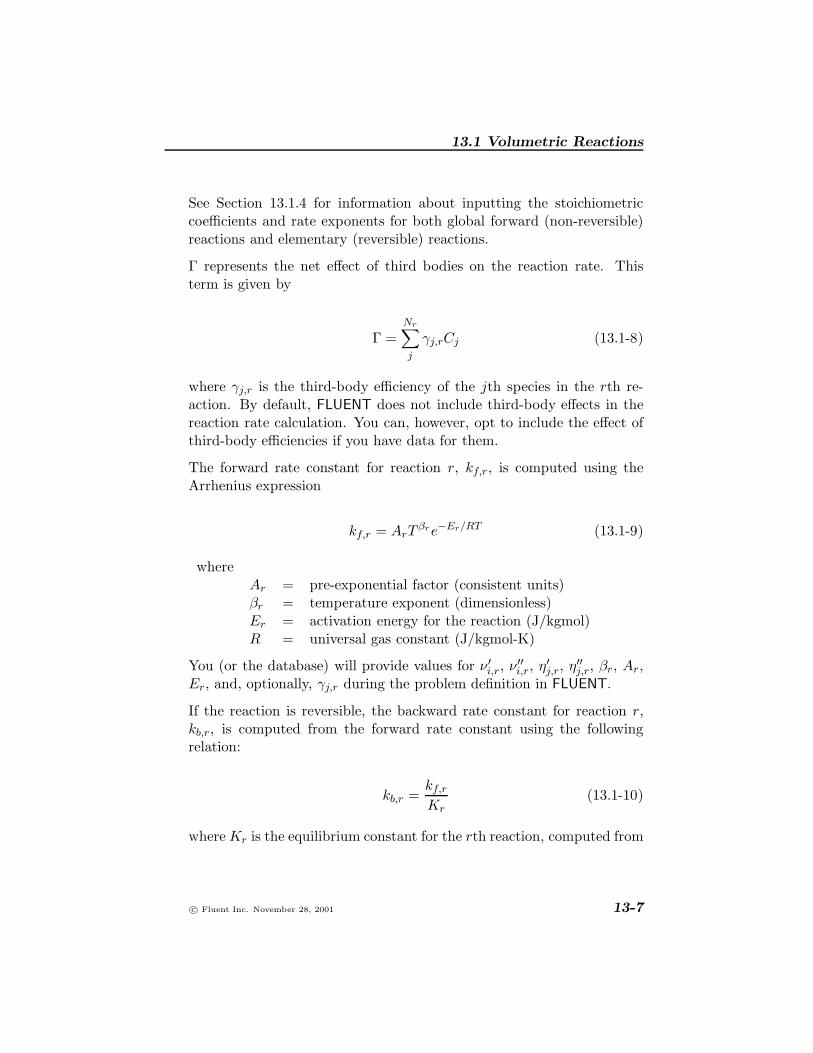
Γ represents the net effect of third bodies on the reaction rate. Thisterm is given by

Γ =Nr∑j

γj,rCj (13.1-8)

where γj,r is the third-body efficiency of the jth species in the rth re-action. By default, FLUENT does not include third-body effects in thereaction rate calculation. You can, however, opt to include the effect ofthird-body efficiencies if you have data for them.

The forward rate constant for reaction r, kf,r, is computed using theArrhenius expression

kf,r = ArTβre−Er/RT (13.1-9)

whereAr = pre-exponential factor (consistent units)βr = temperature exponent (dimensionless)Er = activation energy for the reaction (J/kgmol)R = universal gas constant (J/kgmol-K)

You (or the database) will provide values for ν ′i,r, ν′′i,r, η

′j,r, η

′′j,r, βr, Ar,

Er, and, optionally, γj,r during the problem definition in FLUENT.

If the reaction is reversible, the backward rate constant for reaction r,kb,r, is computed from the forward rate constant using the followingrelation:

kb,r =kf,r

Kr(13.1-10)

whereKr is the equilibrium constant for the rth reaction, computed from



Kr = exp

(∆S0

r

R− ∆H0

r

RT

)(patm

RT

)NR∑r=1

(ν ′′j,r − ν ′j,r)(13.1-11)

where patm denotes atmospheric pressure (101325 Pa). The term withinthe exponential function represents the change in Gibbs free energy, andits components are computed as follows:

∆S0r

R=

N∑i=1

(ν ′′i,r − ν ′i,r

) S0i

R(13.1-12)

∆H0r

RT=

N∑i=1

(ν ′′i,r − ν ′i,r

) h0i

RT(13.1-13)

where S0i and h0

i are the standard-state entropy and standard-state en-thalpy (heat of formation). These values are specified in FLUENT asproperties of the mixture material.

Pressure-Dependent Reactions

FLUENT can use one of three methods to represent the rate expressionin pressure-dependent (or pressure fall-off) reactions. A “fall-off” re-action is one in which the temperature and pressure are such that thereaction occurs between Arrhenius high-pressure and low-pressure limits,and thus is no longer solely dependent on temperature.

There are three methods of representing the rate expressions in thisfall-off region. The simplest one is the Lindemann [140] form. Thereare also two other related methods, the Troe method [77] and the SRImethod [230], that provide a more accurate description of the fall-offregion.

Arrhenius rate parameters are required for both the high- and low-pressure limits. The rate coefficients for these two limits are then blendedto produce a smooth pressure-dependent rate expression. In Arrhenius



form, the parameters for the high-pressure limit (k) and the low-pressurelimit (klow) are as follows:

k = AT βe−E/RT (13.1-14)klow = AlowT

βlowe−Elow/RT (13.1-15)

The net rate constant at any pressure is then taken to be

knet = k

(pr

1 + pr

)F (13.1-16)

where pr is defined as

pr =klow[M ]

k(13.1-17)

and [M ] is the concentration of the bath gas, which can include third-body efficiencies. If the function F in Equation 13.1-16 is unity, then thisis the Lindemann form. FLUENT provides two other forms to describeF , namely the Troe method and the SRI method.

In the Troe method, F is given by

log F =

{1 +

[log pr + c

n− d(log pr + c)

]2}−1

log Fcent (13.1-18)

where

c = −0.4 − 0.67 log Fcent (13.1-19)n = 0.75 − 1.27 log Fcent (13.1-20)d = 0.14 (13.1-21)

and



Fcent = (1 − α)e−T/T3 + αe−T/T1 + e−T2/T (13.1-22)

The parameters α, T3, T2, and T1 are specified as inputs.

In the SRI method, the blending function F is approximated as

F = d

[a exp

(−bT

)+ exp

(−Tc

)]XT e (13.1-23)

where

X =1

1 + log2 pr(13.1-24)

In addition to the three Arrhenius parameters for the low-pressure limit(klow) expression, you must also supply the parameters a, b, c, d, and ein the F expression.

Chemical kinetic mechanisms are usually highly non-linear and form a!set of stiff coupled equations. See Section 13.1.7 for solution procedureguidelines. Also, if you have a chemical mechanism in CHEMKIN [112]format, you can import this mechanism into FLUENT as described inSection 13.1.9.

The Eddy-Dissipation Model

Most fuels are fast burning, and the overall rate of reaction is controlledby turbulent mixing. In non-premixed flames, turbulence slowly con-vects/mixes fuel and oxidizer into the reaction zones where they burnquickly. In premixed flames, the turbulence slowly convects/mixes coldreactants and hot products into the reaction zones, where reaction occursrapidly. In such cases, the combustion is said to be mixing-limited, andthe complex, and often unknown, chemical kinetic rates can be safelyneglected.

FLUENT provides a turbulence-chemistry interaction model, based onthe work of Magnussen and Hjertager [149], called the eddy-dissipation



model. The net rate of production of species i due to reaction r, Ri,r, isgiven by the smaller (i.e., limiting value) of the two expressions below:

Ri,r = ν ′i,rMw,iAρε

kminR

(YR

ν ′R,rMw,R

)(13.1-25)

Ri,r = ν ′i,rMw,iABρε

k

∑P YP∑N

j ν ′′j,rMw,j

(13.1-26)

where YP is the mass fraction of any product species, PYR is the mass fraction of a particular reactant, RA is an empirical constant equal to 4.0B is an empirical constant equal to 0.5

In Equations 13.1-25 and 13.1-26, the chemical reaction rate is governedby the large-eddy mixing time scale, k/ε, as in the eddy-breakup modelof Spalding [227]. Combustion proceeds whenever turbulence is present(k/ε > 0), and an ignition source is not required to initiate combustion.This is usually acceptable for non-premixed flames, but in premixedflames, the reactants will burn as soon as they enter the computationaldomain, upstream of the flame stabilizer. To remedy this, FLUENT pro-vides the finite-rate/eddy-dissipation model, where both the Arrhenius(Equation 13.1-7), and eddy-dissipation (Equations 13.1-25 and 13.1-26)reaction rates are calculated. The net reaction rate is taken as the mini-mum of these two rates. In practice, the Arrhenius rate acts as a kinetic“switch”, preventing reaction before the flame holder. Once the flame isignited, the eddy-dissipation rate is generally smaller than the Arrheniusrate, and reactions are mixing-limited.

Although FLUENT allows multi-step reaction mechanisms (number of!reactions > 2) with the eddy-dissipation and finite-rate/eddy-dissipationmodels, these will likely produce incorrect solutions. The reason is thatmulti-step chemical mechanisms are based on Arrhenius rates, whichdiffer for each reaction. In the eddy-dissipation model, every reaction hasthe same, turbulent rate, and therefore the model should be used only forone-step (reactant → product), or two-step (reactant → intermediate,intermediate → product) global reactions. The model cannot predict



kinetically controlled species such as radicals. To incorporate multi-step chemical kinetic mechanisms in turbulent flows, use the EDC model(described below).

The eddy-dissipation model requires products to initiate reaction (see!Equation 13.1-26). When you initialize the solution, FLUENT sets theproduct mass fractions to 0.01, which is usually sufficient to start thereaction. However, if you converge a mixing solution first, where allproduct mass fractions are zero, you may then have to patch productsinto the reaction zone to ignite the flame. See Section 13.1.7 for details.

The Eddy-Dissipation Model for LES

When the LES turbulence model is used, the turbulent mixing rate, ε/kin Equations 13.1-25 and 13.1-26, is replaced by the subgrid-scale mixingrate. This is calculated as

τ−1sgs =

√2SijSij (13.1-27)

whereτ−1sgs = subgrid-scale mixing rate (s−1)Sij = 1

2

(∂ui∂xj

+ ∂uj

∂xi

)= strain rate tensor (s−1)

The Eddy-Dissipation-Concept (EDC) Model

The eddy-dissipation-concept (EDC) model is an extension of the eddy-dissipation model to include detailed chemical mechanisms in turbulentflows [148]. It assumes that reaction occurs in small turbulent structures,called the fine scales. The volume fraction of the fine scales is modeledas [80]

ξ∗ = Cξ

(νε

k2

)3/4

(13.1-28)

where ∗ denotes fine-scale quantities and

Cξ = volume fraction constant = 2.1377ν = kinematic viscosity



Species are assumed to react in the fine structures over a time scale

τ∗ = Cτ

(ν

ε

)1/2

(13.1-29)

where Cτ is a time scale constant equal to 0.4082.

In FLUENT, combustion at the fine scales is assumed to occur as a con-stant pressure reactor, with initial conditions taken as the current speciesand temperature in the cell. Reactions proceed over the time scale τ∗,governed by the Arrhenius rates of Equation 13.1-7, and are integratednumerically with the stiff ordinary differential equation solver CVODE[45]. The species state after reacting for a time τ∗ is denoted by Y ∗

i .

The source term in the conservation equation for the mean species i,Equation 13.1-1, is modeled as

Ri =ρ(ξ∗)2

τ∗[1 − (ξ∗)3](Y ∗

i − Yi) (13.1-30)

The EDC model can incorporate detailed chemical mechanisms into tur-bulent reacting flows. However, typical mechanisms are invariably stiffand their numerical integration is computationally costly. Hence, themodel should be used only when the assumption of fast chemistry is in-valid, such as modeling the slow CO burnout in rapidly quenched flames,or the NO conversion in selective non-catalytic reduction (SNCR).

The double-precision solver is recommended to avoid round-off errorsthat may occur as a consequence of the large pre-exponential factorsand activation energies inherent in stiff mechanisms. See Section 13.1.7for guidelines on obtaining a solution using the EDC model.



13.1.2 Overview of User Inputs for Modeling Species Transportand Reactions

The basic steps for setting up a problem involving species transport andreactions are listed below, and the details about performing each stepare presented in Sections 13.1.3–13.1.5. Additional information aboutsetting up and solving the problem is provided in Sections 13.1.6–13.1.8.

1. Enable species transport and volumetric reactions, and specify themixture material. See Section 13.1.3. (The mixture material con-cept is explained below.)

2. If you are also modeling wall or particle surface reactions, turnon wall surface and/or particle surface reactions as well. See Sec-tions 13.2 and 13.3 for details.

3. Check and/or define the properties of the mixture. (See Sec-tion 13.1.4.) Mixture properties include the following:

• species in the mixture

• reactions

• other physical properties (e.g., viscosity, specific heat)

4. Check and/or set the properties of the individual species in themixture. (See Section 13.1.4.)

5. Set species boundary conditions. (See Section 13.1.5.)

In many cases, you will not need to modify any physical properties be-cause the solver gets species properties, reactions, etc. from the materialsdatabase when you choose the mixture material. Some properties, how-ever, may not be defined in the database. You will be warned when youchoose your material if any required properties need to be set, and youcan then assign appropriate values for these properties. You may alsowant to check the database values of other properties to be sure thatthey are correct for your particular application. For details about mod-ifying an existing mixture material or creating a new one from scratch,see Section 13.1.4. Modifications to the mixture material can include thefollowing:



• Addition or removal of species

• Changing the chemical reactions

• Modifying other material properties for the mixture

• Modifying material properties for the mixture’s constituent species

If you are solving a reacting flow, you will usually want to define the mix-ture’s specific heat as a function of composition, and the specific heat ofeach species as a function of temperature. You may want to do the samefor other properties as well. By default, constant properties are used, butfor the properties of some species, there is a piecewise-polynomial func-tion of temperature that exists in the database and is available for youruse. You may also choose to specify a different temperature-dependentfunction if you know of one that is more suitable for your problem.

Mixture Materials

The concept of mixture materials has been implemented in FLUENTto facilitate the setup of species transport and reacting flow. A mixturematerial may be thought of as a set of species and a list of rules governingtheir interaction. The mixture material carries with it the followinginformation:

• A list of the constituent species, referred to as “fluid” materials

• A list of mixing laws dictating how mixture properties (density,viscosity, specific heat, etc.) are to be derived from the properties ofindividual species if composition-dependent properties are desired

• A direct specification of mixture properties if composition-indepen-dent properties are desired

• Diffusion coefficients for individual species in the mixture

• Other material properties (e.g., absorption and scattering coeffi-cients) that are not associated with individual species



• A set of reactions, including a reaction type (finite-rate, eddy-dissipation, etc.) and stoichiometry and rate constants

Both mixture materials and fluid materials are stored in the FLUENTmaterials database. Many common mixture materials are included (e.g.,methane-air, propane-air). Generally, one/two-step reaction mechanismsand many physical properties of the mixture and its constituent speciesare defined in the database. When you indicate which mixture materialyou want to use, the appropriate mixture material, fluid materials, andproperties are loaded into the solver. If any necessary information aboutthe selected material (or the constituent fluid materials) is missing, thesolver will inform you that you need to specify it. In addition, you maychoose to modify any of the predefined properties. See Section 7.1.2 forinformation about the sources of FLUENT’s database property data.

For example, if you plan to model combustion of a methane-air mixture,you do not need to explicitly specify the species involved in the reactionor the reaction itself. You will simply select methane-air as the mixturematerial to be used, and the relevant species (CH4, O2, CO2, H2O, andN2) and reaction data will be loaded into the solver from the database.You can then check the species, reactions, and other properties and defineany properties that are missing and/or modify any properties for whichyou wish to use different values or functions. You will generally wantto define a composition- and temperature-dependent specific heat, andyou may want to define additional properties as functions of temperatureand/or composition.

The use of mixture materials gives you the flexibility to use one of themany predefined mixtures, modify one of these mixtures, or create yourown mixture material. Customization of mixture materials is performedin the Materials panel, as described in Section 13.1.4.



13.1.3 Enabling Species Transport and Reactions and Choosingthe Mixture Material

The problem setup for species transport and volumetric reactions beginsin the Species Model panel (Figure 13.1.1).

Define −→ Models −→Species...

Figure 13.1.1: The Species Model Panel

1. Under Model, select Species Transport.

2. Under Reactions, turn on Volumetric Reactions.

3. In the Mixture Material drop-down list under Mixture Properties,choose which mixture material you want to use in your problem.



The drop-down list will include all of the mixtures that are cur-rently defined in the database. To check the properties of a mixturematerial, select it and click the View... button. If the mixture youwant to use is not in the list, choose the mixture-template material,and see Section 13.1.4 for details on setting your mixture’s proper-ties. If there is a mixture material listed that is similar to your de-sired mixture, you may choose that material and see Section 13.1.4for details on modifying properties of an existing material.

When you choose the Mixture Material, the Number of Volumet-ric Species in the mixture will be displayed in the panel for yourinformation.

Note that if you re-open the Species Model panel after species trans-!port has already been enabled, only the mixture materials avail-able in your case will appear in the list. You can add more mixturematerials to your case by copying them from the database, as de-scribed in Section 7.1.2, or by creating a new mixture, as describedin Sections 7.1.2 and 13.1.4.

As mentioned in Section 13.1.2, modeling parameters for the speciestransport and (if relevant) reactions will automatically be loadedfrom the database. If any information is missing, you will be in-formed of this after you click on OK in the Species Model panel. Ifyou want to check or modify any properties of the mixture material,you will use the Materials panel, as described in Section 13.1.4.

4. Choose the Turbulence-Chemistry Interaction model. Four modelsare available:

Laminar Finite-Rate computes only the Arrhenius rate (see Equa-tion 13.1-7) and neglects turbulence-chemistry interaction.

Eddy-Dissipation (for turbulent flows) computes only the mixingrate (see Equations 13.1-25 and 13.1-26).

Finite-Rate/Eddy-Dissipation (for turbulent flows) computes boththe Arrhenius rate and the mixing rate and uses the smallerof the two.

EDC (for turbulent flows) models turbulence-chemistry interactionwith detailed chemical mechanisms (see Equations 13.1-25



and 13.1-26).

5. If you selected EDC, you have the option to modify the Volume Frac-tion Constant and the Time Scale Constant (Cξ in Equation 13.1-28and Cτ in Equation 13.1-29), although the default values are rec-ommended. Further, to reduce the computational expense of thechemistry calculations, you can increase the number of Flow Itera-tions Per Chemistry Update. By default, FLUENT will update thechemistry one per 10 flow iterations.

6. (optional) If you want to model full multicomponent diffusion orthermal diffusion, turn on the Full Multicomponent Diffusion orThermal Diffusion option. See Section 7.7.2 for details.

13.1.4 Defining Properties for the Mixture and Its ConstituentSpecies

As discussed in Section 13.1.2, if you use a mixture material from thedatabase, most mixture and species properties will already be defined.You may follow the procedures in this section to check the current prop-erties, modify some of the properties, or set all properties for a brand-newmixture material that you are defining from scratch.

Remember that you will need to define properties for the mixture mate-rial and also for its constituent species. It is important that you definethe mixture properties before setting any properties for the constituentspecies, since the species property inputs may depend on the methodsyou use to define the properties of the mixture. The recommended se-quence for property inputs is as follows:

1. Define the mixture species, and reaction(s), and define physicalproperties for the mixture. Remember to click on the Change/Createbutton when you are done setting properties for the mixture ma-terial.

2. Define physical properties for the species in the mixture. Remem-ber to click on the Change/Create button after defining the prop-erties for each species.



These steps, all of which are performed in the Materials panel, are de-scribed in detail in this section.

Define −→Materials...

Defining the Species in the Mixture

If you are using a mixture material from the database, the species in themixture will already be defined for you. If you are creating your ownmaterial or modifying the species in an existing material, you will needto define them yourself.

In the Materials panel (Figure 13.1.2), check that the Material Type isset to mixture and your mixture is selected in the Mixture Materials list.Click on the Edit... button to the right of Mixture Species to open theSpecies panel (Figure 13.1.3).

Overview of the Species Panel

In the Species panel, the Selected Species list shows all of the fluid-phasespecies in the mixture. If you are modeling wall or particle surface reac-tions, the Selected Surface Species list will show all of the surface speciesin the mixture. Surface species are species that are created or evolvedfrom wall boundaries or discrete-phase particles (e.g., Si(s)) and do notexist as fluid-phase species. The use of surface species and wall surfacereactions is described in Section 13.2. See Section 13.3 for informationabout particle surface reactions.

The order of the species in the Selected Species list is very important.!FLUENT considers the last species in the list to be the bulk species.You should therefore be careful to retain the most abundant species (bymass) as the last species when you add species to or delete species froma mixture material.

The Available Materials list shows materials that are available but not inthe mixture. Generally you will see air in this list, since air is alwaysavailable by default.



Figure 13.1.2: The Materials Panel (showing a mixture material)



Figure 13.1.3: The Species Panel

Adding Species to the Mixture

If you are creating a mixture from scratch or starting from an existingmixture and adding some missing species, you will first need to loadthe desired species from the database (or create them, if they are notpresent in the database) so that they will be available to the solver. Theprocedure for adding species is listed below. (You will need to close theSpecies panel before you begin, since it is a “modal” panel that will notallow you to do anything else when it is open.)

1. In the Materials panel, click on the Database... button to openthe Database Materials panel and copy the desired species, as de-scribed in Section 7.1.2. Remember that the constituent speciesof the mixture are fluid materials, so you should select fluid as the



Material Type in the Database Materials panel to see the correct listof choices. Note that available solid species (for surface reactions)are also contained in the fluid list.

If you do not see the species you are looking for in the database,!you can create a new fluid material for that species, following theinstructions in Section 7.1.2, and then continue with step 2, below.

2. Re-open the Species panel, as described above. You will see thatthe fluid materials you copied from the database (or created) arelisted in the Available Materials list.

3. To add a species to the mixture, select it in the Available Materialslist and click on the Add button below the Selected Species list (orbelow the Selected Surface Species list, to define a surface species).The species will be added to the end of the Selected Species (or Se-lected Surface Species) list and removed from the Available Materialslist.

4. Repeat the previous step for all the desired species. When you arefinished, click on the OK button.

Adding a species to the list will alter the order of the species. You!should be sure that the last species in the list is the bulk species, andyou should check any boundary conditions, under-relaxation factors, orother solution parameters that you have set, as described in detail below.

Removing Species from the Mixture

To remove a species from the mixture, simply select it in the SelectedSpecies list (or the Selected Surface Species list) and click on the Removebutton below the list. The species will be removed from the list andadded to the Available Materials list.

Removing a species from the list will alter the order of the species. You!should be sure that the last species in the list is the bulk species, andyou should check any boundary conditions, under-relaxation factors, orother solution parameters that you have set, as described in detail below.



Reordering Species

If you find that the last species in the Selected Species list is not the mostabundant species (as it must be), you will need to rearrange the speciesto obtain the proper order.

1. Remove the bulk species from the Selected Species list. It will nowappear in the Available Species list.

2. Add the species back in again. It will automatically be placed atthe end of the list.

The Naming and Ordering of Species

As discussed above, you must retain the most abundant species as thelast one in the Selected Species list when you add or remove species. Ad-ditional considerations you should be aware of when adding and deletingspecies are presented here.

There are three characteristics of a species that identify it to the solver:name, chemical formula, and position in the list of species in the Speciespanel. Changing these characteristics will have the following effects:

• You can change the Name of a species (using the Materials panel,as described in Section 7.1.2) without any consequences.

• You should never change the given Chemical Formula of a species.

• You will change the order of the species list if you add or removeany species. When this occurs, all boundary conditions, solver pa-rameters, and solution data for species will be reset to the defaultvalues. (Solution data, boundary conditions, and solver parame-ters for other flow variables will not be affected.) Thus, if you addor remove species you should take care to redefine species boundaryconditions and solution parameters for the newly defined problem.In addition, you should recognize that patched species concentra-tions or concentrations stored in any data file that was based onthe original species ordering will be incompatible with the newly



defined problem. You can use the data file as a starting guess, butyou should be aware that the species concentrations in the datafile may provide a poor initial guess for the newly defined model.

Defining Reactions

If your FLUENT model involves chemical reactions, you can next definethe reactions in which the defined species participate. This will be nec-essary only if you are creating a mixture material from scratch, you havemodified the species, or you want to redefine the reactions for some otherreason.

Depending on which turbulence-chemistry interaction model you selectedin the Species Model panel (see Section 13.1.3), the appropriate reactionmechanism will be displayed in the Reaction drop-down list in the Mate-rials panel. If you are using the laminar finite-rate or EDC model, the re-action mechanism will be finite-rate; if you are using the eddy-dissipationmodel, the reaction mechanism will be eddy-dissipation; if you are usingthe finite-rate/eddy-dissipation model, the reaction mechanism will befinite-rate/eddy-dissipation.

Inputs for Reaction Definition

To define the reactions, click on the Edit... button to the right of Reaction.The Reactions panel (Figure 13.1.4) will open.

The steps for defining reactions are as follows:

1. Set the total number of reactions (volumetric reactions, wall surfacereactions, and particle surface reactions) in the Total Number ofReactions field. (Use the arrows to change the value, or type in thevalue and press RETURN.)

Note that if your model includes discrete-phase combusting par-ticles, you should include the particulate surface reaction(s) (e.g.,char burnout, multiple char oxidation) in the number of reactionsonly if you plan to use the multiple surface reactions model forsurface combustion.



Figure 13.1.4: The Reactions Panel



2. Set the Reaction ID of the reaction you want to define. (Again, ifyou type in the value be sure to press RETURN.)

3. If this is a fluid-phase reaction, keep the default selection of Vol-umetric as the Reaction Type. If this is a wall surface reaction(described in Section 13.2) or a particle surface reaction (describedin Section 13.3), select Wall Surface or Particle Surface as the Reac-tion Type. See Section 13.3.2 for further information about definingparticle surface reactions.

4. Specify how many reactants and products are involved in the re-action by increasing the value of the Number of Reactants and theNumber of Products. Select each reactant or product in the Speciesdrop-down list and then set its stoichiometric coefficient and rateexponent in the appropriate Stoich. Coefficient and Rate Exponentfields. (The stoichiometric coefficient is the constant ν ′i,r or ν ′′i,rin Equation 13.1-6 and the rate exponent is the exponent on thereactant or product concentration, η′j,r or η′′j,r in Equation 13.1-7.)

There are two general classes of reactions that can be handled bythe Reactions panel, so it is important that the parameters foreach reaction are entered correctly. The classes of reactions are asfollows:

• Global forward reaction (no reverse reaction): Product speciesgenerally do not affect the forward rate, so the rate exponentfor all products (η′′j,r) should be 0. For reactant species, setthe rate exponent (η′j,r) to the desired value. If such a re-action is not an elementary reaction, the rate exponent willgenerally not be equal to the stoichiometric coefficient (ν ′i,r)for that species. An example of a global forward reaction isthe combustion of methane:

CH4 + 2O2 −→ CO2 + 2H2O

where ν ′CH4= 1, η′CH4

= 0.2, ν ′O2= 2, η′O2

= 1.3, ν ′′CO2= 1,

η′′CO2= 0, ν ′′H2O

= 2, and η′′H2O = 0.

Figure 13.1.4 shows the coefficient inputs for the combustionof methane. (See also the methane-air mixture material in the



Database Materials panel.)

Note that, in certain cases, you may wish to model a reactionwhere product species affect the forward rate. For such cases,set the product rate exponent (η′′j,r) to the desired value. Anexample of such a reaction is the gas-shift reaction (see thecarbon-monoxide-air mixture material in the Database Materi-als panel), in which the presence of water has an effect on thereaction rate:

CO + 12O2 + H2O −→ CO2 + H2O

In the gas-shift reaction, the rate expression may be definedas:

k[CO][O2]1/4[H2O]1/2

where ν ′CO = 1, η′CO = 1, ν ′O2= 0.5, η′O2

= 0.25, ν ′′CO2= 1,

η′′CO2= 0, ν ′′H2O

= 0, and η′′H2O = 0.5.

• Reversible reaction: An elementary chemical reaction thatassumes the rate exponent for each species is equivalent tothe stoichiometric coefficient for that species. An example ofan elementary reaction is the oxidation of SO2 to SO3:

SO2 + 12O2 ⇀↽ SO3

where ν ′SO2= 1, η′SO2

= 1, ν ′O2= 0.5, η′O2

= 0.5, ν ′′SO3= 1,

and η′′SO3= 1.

See step 6 below for information about how to enable re-versible reactions.

5. If you are using the laminar finite-rate, finite-rate/eddy-dissipation,or EDC model for the turbulence-chemistry interaction, enter thefollowing parameters for the Arrhenius rate under the ArrheniusRate heading:

Pre-exponential Factor (the constant Ar in Equation 13.1-9). Theunits of Ar must be specified such that the units of the mo-lar reaction rate, Ri,r in Equation 13.1-5, are moles/volume-time (e.g., kgmol/m3-s) and the units of the volumetric reac-



tion rate, Ri in Equation 13.1-5, are mass/volume-time (e.g.,kg/m3-s).

It is important to note that if you have selected the British!units system, the Arrhenius factor should still be input in SIunits. This is because FLUENT applies no conversion factorto your input of Ar (the conversion factor is 1.0) when youwork in British units, as the correct conversion factor dependson your inputs for ν ′i,r, βr, etc.

Activation Energy (the constant Er in the forward rate constantexpression, Equation 13.1-9).

Temperature Exponent (the value for the constant βr in Equation13.1-9).

Third Body Efficiencies (the values for γj,r in Equation 13.1-8). Ifyou have accurate data for the efficiencies and want to in-clude this effect on the reaction rate (i.e., include Γ in Equa-tion 13.1-7), turn on the Third Body Efficiencies option andclick on the Specify... button to open the Reaction Parameterspanel (Figure 13.1.5). For each Species in the panel, specifythe Third-body Efficiency.

It is not necessary to include the third-body efficiencies. You!should not enable the Third Body Efficiencies option unless youhave accurate data for these parameters.

Pressure Dependent Reaction (if relevant) If you are using the lam-inar finite-rate or EDC model for turbulence-chemistry in-teraction, and the reaction is a pressure fall-off reaction (seeSection 13.1.1), turn on the Pressure Dependent Reaction op-tion for the Arrhenius Rate and click on the Specify... button toopen the Pressure-Dependent Reaction panel (Figure 13.1.6).

Under Reaction Parameters, select the appropriate ReactionType (lindemann, troe, or sri). See Section 13.1.1 for detailsabout the three methods. Next, you must specify if the BathGas Concentration ([M ] in Equation 13.1-17) is to be definedas the concentration of the mixture, or as the concentrationof one of the mixture’s constituent species, by selecting theappropriate item in the drop-down list.



Figure 13.1.5: The Reaction Parameters Panel

The parameters you specified under Arrhenius Rate in the Re-actions panel represent the high-pressure Arrhenius parame-ters. You can, however, specify values for the following pa-rameters under Low Pressure Arrhenius Rate:

ln(Pre-exponential Factor) (Alow in Equation 13.1-15) The pre-exponential factor Alow is often an extremely large num-ber, so you will input the natural logarithm of this term.

Activation Energy (Elow in Equation 13.1-15)

Temperature Exponent (βlow in Equation 13.1-15)

If you selected troe for the Reaction Type, you can specifyvalues for Alpha, T1, T2, and T3 (α, T1, T2, and T3 in Equa-tion 13.1-22) under Troe parameters. If you selected sri for theReaction Type, you can specify values for a, b, c, d, and e (a,b, c, d, and e in Equation 13.1-23) under SRI parameters.



Figure 13.1.6: The Pressure-Dependent Reaction Panel



6. If you are using the laminar finite-rate or EDC model for turbulence-chemistry interaction, and the reaction is reversible, turn on theInclude Backward Reaction option for the Arrhenius Rate. When thisoption is enabled, you will not be able to edit the Rate Exponentfor the product species, which instead will be set to be equiva-lent to the corresponding product Stoich. Coefficient. If you donot wish to use FLUENT’s default values, or if you are definingyour own reaction, you will also need to specify the standard-stateenthalpy and standard-state entropy, to be used in the calcula-tion of the backward reaction rate constant (Equation 13.1-10).Note that the reversible reaction option is not available for eitherthe eddy-dissipation or the finite-rate/eddy-dissipation turbulence-chemistry interaction model.

7. If you are using the eddy-dissipation or finite-rate/eddy-dissipationmodel for turbulence-chemistry interaction, you can enter valuesfor A and B under the Mixing Rate heading. Note, however, thatthese values should not be changed unless you have reliable data.In most cases you will simply use the default values.

A is the constant A in the turbulent mixing rate (Equations 13.1-25and 13.1-26) when it is applied to a species that appears as areactant in this reaction. The default setting of 4.0 is based on theempirically derived values given by Magnussen et al. [149].

B is the constant B in the turbulent mixing rate (Equation 13.1-26)when it is applied to a species that appears as a product in thisreaction. The default setting of 0.5 is based on the empiricallyderived values given by Magnussen et al. [149].

8. Repeat steps 2–7 for each reaction you need to define. When youare finished defining all reactions, click OK.

Defining Species and Reactions for Fuel Mixtures

Quite often, combustion systems will include fuel that is not easily de-scribed as a pure species (such as CH4 or C2H6). Complex hydrocarbons,including fuel oil or even wood chips, may be difficult to define in termsof such pure species. However, if you have available the heating value



and the ultimate analysis (elemental composition) of the fuel, you candefine an equivalent fuel species and an equivalent heat of formation forthis fuel. Consider, for example, a fuel known to contain 50% C, 6%H, and 44% O by weight. Dividing by atomic weights, you can arriveat a “fuel” species with the molecular formula C4.17H6O2.75. You canstart from a similar, existing species or create a species from scratch,and assign it a molecular weight of 100.04 (4.17 × 12 + 6 × 1 + 2.75 ×16). The chemical reaction would be considered to be

C4.17H6O2.75 + 4.295O2 −→ 4.17CO2 + 3H2O

You will need to set the appropriate stoichiometric coefficients for thisreaction.

The heat of formation (or standard-state enthalpy) for the fuel speciescan be calculated from the known heating value ∆H since

∆H =N∑

i=1

h0i

(ν ′′i,r − ν ′i,r

)(13.1-31)

where h0i is the standard-state enthalpy on a molar basis. Note the sign

convention in Equation 13.1-31: ∆H is negative when the reaction isexothermic.

Defining Physical Properties for the Mixture

When your FLUENT model includes chemical species, the following phys-ical properties must be defined, either by you or by the database, for themixture material:

• density, which you can define using the gas law or as a volume-weighted function of composition

• viscosity, which you can define as a function of composition

• thermal conductivity and specific heat (in problems involving so-lution of the energy equation), which you can define as functionsof composition.



• mass diffusion coefficients and Schmidt number, which govern themass diffusion fluxes (Equations 13.1-2 and 13.1-3)

Detailed descriptions of these property inputs are provided in Chapter 7.

Remember to click on the Change/Create button when you are done!setting the properties of the mixture material. The properties that ap-pear for each of the constituent species will depend on your settings forthe properties of the mixture material. If, for example, you specify acomposition-dependent viscosity for the mixture, you will need to defineviscosity for each species.

Defining Physical Properties for the Species in the Mixture

For each of the fluid materials in the mixture, you (or the database)must define the following physical properties:

• molecular weight, which is used in the gas law and/or in the cal-culation of reaction rates and mole-fraction inputs or outputs

• standard-state (formation) enthalpy and reference temperature (inproblems involving solution of the energy equation)

• viscosity, if you defined the viscosity of the mixture material as afunction of composition

• thermal conductivity and specific heat (in problems involving so-lution of the energy equation), if you defined these properties ofthe mixture material as functions of composition

• standard-state entropy, if you are modeling reversible reactions

Detailed descriptions of these property inputs are provided in Chapter 7.

Global reaction mechanisms with one or two steps inevitably neglect!the intermediate species. In high-temperature flames, neglecting thesedissociated species may cause the temperature to be overpredicted. Amore realistic temperature field can be obtained by increasing the specificheat capacity for each species. Rose and Cooper [252] have created a set



of specific heat polynomials as a function of temperature. The specificheat capacity for each species is calculated as

cp(T ) =m∑

k=0

akTk (13.1-32)

The modified cp polynomial coefficients from [252] are provided in Ta-ble 13.1.1.

Table 13.1.1: Modified cp Polynomial Coefficients [252]N2 CH4 CO H2

a0 1.02705e+03 2.00500e+03 1.04669e+03 1.4147e+04a1 2.16182e−02 −6.81428e−01 −1.56841e−01 1.7372e−01a2 1.48638e−04 7.08589e−03 5.39904e−04 6.9e−04a3 −4.48421e−08 −4.71368e−06 −3.01061e−07 —–a4 —– 8.51317e−10 5.05048e−11 —–

CO2 H2O O2

a0 5.35446e+02 1.93780e+03 8.76317e+02a1 1.27867e+00 −1.18077e+00 1.22828e−01a2 −5.46776e−04 3.64357e−03 5.58304e−04a3 −2.38224e−07 −2.86327e−06 −1.20247e−06a4 1.89204e−10 7.59578e−10 1.14741e−09a5 —– —– −5.12377e−13a6 —– —– 8.56597e−17

13.1.5 Defining Boundary Conditions for Species

You will need to specify the inlet mass fraction for each species in yoursimulation. In addition, for pressure outlets you will set species massfractions to be used in case of backflow at the exit. At walls, FLUENTwill apply a zero-gradient (zero-flux) boundary condition for all speciesunless you have defined a surface reaction at that wall (see Section 13.2)or you choose to specify species mass fractions at the wall. Input ofboundary conditions is described in Chapter 6.

Note that you will explicitly set mass fractions only for the first N − 1!



species. The solver will compute the mass fraction of the last speciesby subtracting the total of the specified mass fractions from 1. If youwant to explicitly specify the mass fraction of the last species, you mustreorder the species in the list (in the Materials panel), as described inSection 13.1.4.

Diffusion at Inlets with the Segregated Solver

As noted in Section 13.1.1, the species diffusion component at inlets(and therefore the net inlet transport) is not specified when the segre-gated solver is used. In some cases, you may wish to include only theconvective transport of species through the inlets of your domain. Youcan do this by disabling inlet species diffusion. By default, FLUENT in-cludes the diffusion flux of species at inlets. To turn off inlet diffusion,use the define/models/species-transport/inlet-diffusion? textcommand.

13.1.6 Defining Other Sources of Chemical Species

You can define a source or sink of a chemical species within the compu-tational domain by defining a source term in the Fluid panel. You maychoose this approach when species sources exist in your problem but youdo not want to model them through the mechanism of chemical reac-tions. Section 6.27 describes the procedures you follow to define speciessources in your FLUENT model. If the source is not a constant, you canuse a user-defined function. See the separate UDF Manual for detailsabout user-defined functions.

13.1.7 Solution Procedures for Chemical Mixing andFinite-Rate Chemistry

While many simulations involving chemical species may require no spe-cial procedures during the solution process, you may find that one ormore of the solution techniques noted in this section helps to acceler-ate the convergence or improve the stability of more complex simula-tions. The techniques outlined below may be of particular importance if



your problem involves many species and/or chemical reactions, especiallywhen modeling combusting flows.

Stability and Convergence in Reacting Flows

Obtaining a converged solution in a reacting flow can be difficult for anumber of reasons. First, the impact of the chemical reaction on thebasic flow pattern may be strong, leading to a model in which there isstrong coupling between the mass/momentum balances and the speciestransport equations. This is especially true in combustion, where thereactions lead to a large heat release and subsequent density changes andlarge accelerations in the flow. All reacting systems have some degreeof coupling, however, when the flow properties depend on the speciesconcentrations. These coupling issues are best addressed by the use of atwo-step solution process, as described below, and by the use of under-relaxation as described in Section 22.9.

A second convergence issue in reacting flows involves the magnitude ofthe reaction source term. When your FLUENT model involves very rapidreaction rates (i.e., much more rapid than the rates of convection anddiffusion), the solution of the species transport equations becomes nu-merically difficult. Such systems are termed “stiff” systems and arecreated when you define models that involve very rapid kinetic rates, es-pecially when these rates describe reversible or competing reactions. Inthe eddy-dissipation model, the fast reaction rates are removed by usingthe slower turbulent rates. For non-premixed systems, reaction rates areeliminated from the model. For stiff systems with laminar chemistry,the coupled solver is recommended instead of the segregated solver. Fora turbulent finite-rate mechanism (which can be stiff), the EDC model,which uses a stiff ODE integrator for the chemistry, is recommended.See below for additional guidelines for solving stiff chemistry systems.

Two-Step Solution Procedure (Cold Flow Simulation)

Solving a reacting flow as a two-step process can be a practical methodfor reaching a stable converged solution to your FLUENT problem. In thisprocess, you begin by solving the flow, energy, and species equations withreactions disabled (the “cold-flow”, or unreacting flow). When the basic



flow pattern has thus been established, you can re-enable the reactionsand continue the calculation. The cold-flow solution provides a goodstarting solution for the calculation of the combusting system. Thistwo-step approach to combustion modeling can be accomplished usingthe following procedure:

1. Set up the problem including all species and reactions of interest.

2. Temporarily disable reaction calculations by turning off VolumetricReactions in the Species Model panel.


3. Turn off calculation of the product species in the Solution Controlspanel.

Solve −→ Controls −→Solution...

4. Calculate an initial (cold-flow) solution. (Note that it is generallynot productive to obtain a fully converged cold-flow solution unlessthe non-reacting solution is also of interest to you.)

5. Enable the reaction calculations by turning on Volumetric Reactionsagain in the Species Model panel.

6. Turn on all equations. If you are using the laminar finite-rate,finite-rate/eddy-dissipation, or EDC model for turbulence-chemistry interaction, you may need to patch an ignition source(as described below).

Density Under-Relaxation

One of the main reasons a combustion calculation can have difficultyconverging is that large changes in temperature cause large changes indensity, which can, in turn, cause instabilities in the flow solution. Whenyou use the segregated solver, FLUENT allows you to under-relax thechange in density to alleviate this difficulty. The default value for densityunder-relaxation is 1, but if you encounter convergence trouble you maywish to reduce this to a value between 0.5 and 1 (in the Solution Controlspanel).



Ignition in Combustion Simulations

If you introduce fuel to an oxidant, spontaneous ignition does not oc-cur unless the temperature of the mixture exceeds the activation energythreshold required to maintain combustion. This physical issue mani-fests itself in a FLUENT simulation as well. If you are using the laminarfinite-rate, finite-rate/eddy-dissipation, or EDC model for turbulence-chemistry interaction, you have to supply an ignition source to initiatecombustion. This ignition source may be a heated surface or inlet massflow that heats the gas mixture above the required ignition temperature.Often, however, it is the equivalent of a spark: an initial solution statethat causes combustion to proceed. You can supply this initial sparkby patching a hot temperature into a region of the FLUENT model thatcontains a sufficient fuel/air mixture for ignition to occur.

Solve −→ Initialize −→Patch...

Depending on the model, you may need to patch both the tempera-ture and the fuel/oxidant/product concentrations to produce ignition inyour model. The initial patch has no impact on the final steady-statesolution—no more than the location of a match determines the final flowpattern of the torch that it lights. See Section 22.13.2 for details aboutpatching initial values.

Solution of Stiff Laminar Chemistry Systems

When modeling laminar reaction systems with the laminar finite-ratemodel, you will likely need to use the coupled solver when the chemicalmechanism is stiff. (See the above discussion on solution convergence inreacting flows. Note that you can use the laminar finite-rate model forturbulent flames, which implies that turbulence-chemistry interactionsare neglected.) In addition, you can provide further solution stability forthe coupled solver by using the stiff-chemistry text command.

solve −→ set −→stiff-chemistry

This option allows a larger Courant (CFL) number specification, al-though additional calculations are required to calculate the eigenvaluesof the chemical Jacobian [258]. When you enable the stiff-chemistrysolver, you will be asked to specify the following:



• Positivity rate limit for temperature: limits new temperature changesby this factor multiplied by the old temperature. Its default valueis 0.2.

• Temperature time-step reduction factor: limits the local CFL num-ber when the temperature is changing too rapidly. Its default valueis 0.25.

• Maximum allowable time-step/chemical-time-scale ratio: limits thelocal CFL number when the chemical time scales (eigenvalues of thechemical Jacobian) become too large to maintain a well-conditionedmatrix. Its default value is 0.9.

The default values of these parameters are applicable in most cases.

Note that the stiff-chemistry option is not available with the segre-gated solver; it can be used only with the coupled solver (either implicitor explicit).

EDC Model Solution Procedure

If you are using the EDC model, it is recommended that you use thedouble-precision solver (see Section 1.5) to avoid round-off errors thatmay occur as a consequence of the large pre-exponential factors andactivation energies that are inherent in stiff mechanisms.

Due to the high computational expense of the EDC model, it is recom-mended that you use the following procedure to obtain a solution usingthe segregated solver:

1. Calculate an initial solution using the eddy-dissipation model anda simple one-step or two-step heat release mechanism.

2. Enable the EDC chemical mechanism with the appropriate species.If you have a mechanism in CHEMKIN [112] format, see Sec-tion 13.1.9 for details on how to import it.

3. If the number of species or their reaction order has changed, youwill need to change the species boundary conditions.

Define −→Boundary Conditions...



4. Temporarily disable reaction calculations by turning off VolumetricReactions in the Species Model panel.


5. Enable solution of only the species equations in the Solution Con-trols panel.

Solve −→ Controls −→Solution...

6. Calculate a solution for the species mixing field.

7. Enable the reaction calculations by turning on Volumetric Reactionsin the Species Model panel and selecting the EDC model underTurbulence-Chemistry Interaction.

8. Enable solution of the Energy equation in the Solution Controlspanel.

9. Calculate a solution for the combined species and temperaturefields. You may have to patch in a high-temperature region ifthe flame blows off.

10. Turn on all equations.

11. Calculate a final solution.

13.1.8 Postprocessing for Species Calculations

FLUENT can report chemical species as mass fractions, mole fractions,and molar concentrations. You can also display laminar and effectivemass diffusion coefficients. The following variables are available for post-processing of species transport and reaction simulations:

• Mass fraction of species-n

• Mole fraction of species-n

• Concentration of species-n

• Lam Diff Coef of species-n



• Eff Diff Coef of species-n

• Thermal Diff Coef of species-n

• Enthalpy of species-n (segregated solver calculations only)

• species-n Source Term (segregated solver calculations only)

• Surface Deposition Rate of species-n (particle surface reaction cal-culations only)

• Relative Humidity

• Time Step Scale (stiff-chemistry solver only)

• Fine Scale Mass fraction of species-n (EDC model only)

• Fine Scale Transfer Rate (EDC model only)

• 1-Fine Scale Volume Fraction (EDC model only)

• Fine Scale Temperature (EDC model only)

• Rate of Reaction-n

• Arrhenius Rate of Reaction-n

• Turbulent Rate of Reaction-n

These variables are contained in the Species..., Temperature..., and Reac-tions... categories of the variable selection drop-down list that appearsin postprocessing panels. See Chapter 27 for a complete list of flow vari-ables, field functions, and their definitions. Chapters 25 and 26 explainhow to generate graphics displays and reports of data.

Averaged Species Concentrations

Averaged species concentrations at inlets and exits, and across selectedplanes (i.e., surfaces that you have created using the Surface menu items)within your model can be obtained using the Surface Integrals panel, asdescribed in Section 26.5.



Report −→Surface Integrals...

Select the Concentration of species-n for the appropriate species in theField Variable drop-down list.

13.1.9 Importing a Chemical Mechanism from CHEMKIN

If you have a gas-phase chemical mechanism in CHEMKIN [112] format,you can import the mechanism files into FLUENT using the ChemkinImport panel (Figure 13.1.7).

File −→ Import −→Chemkin...

Figure 13.1.7: The Chemkin Import Panel

In the Chemkin Import panel, enter the path to the CHEMKIN file (e.g.,path/file.che) under Chemkin Mechanism File and specify the locationof the Thermodynamic Data File (THERMO.DB). See Section 14.3.1 for moreinformation about this database.

When you have specified the correct path for both files, enter a namefor the chemical mechanism under Material Name and click the Importbutton. FLUENT will create a material with the specified name, whichwill contain the CHEMKIN data for the species and reactions, and addit to the list of available Mixture Materials in the Materials panel.



13.2 Wall Surface Reactions and Chemical VaporDeposition

For gas-phase reactions, the reaction rate is defined on a volumetric basisand the rate of creation and destruction of chemical species becomes asource term in the species conservation equations. The rate of depositionis governed by both chemical kinetics and the diffusion rate from the fluidto the surface. Wall surface reactions thus create sources (and sinks) ofchemical species in the bulk phase and determine the rate of depositionof surface species.

Information about wall surface reactions and chemical vapor depositionis presented in the following subsections:

• Section 13.2.1: Overview and Limitations


• Section 13.2.3: User Inputs for Wall Surface Reactions

• Section 13.2.4: Solution Procedures for Wall Surface Reactions

• Section 13.2.5: Postprocessing for Wall Surface Reactions

13.2.1 Overview and Limitations

Overview of Surface Species and Wall Surface Reactions

FLUENT treats chemical species deposited on surfaces as distinct fromthe same chemical species in the gas. Similarly, reactions involving sur-face deposition are defined as distinct surface reactions and hence treateddifferently than bulk phase reactions involving the same chemical species.Consider, for example, the following reaction mechanism for silicon de-position from silane:

Reaction 1 (surface): SiH4(g) → Si(s) + 2 H2(g)Reaction 2 (gas): SiH4(g) → Si H2(g) + H2(g)Reaction 3 (gas): SiH2(g) → Si(g) + H2(g)Reaction 4 (surface): SiH2(g) → Si(s) + H2(g)Reaction 5 (surface): Si(g) → Si(s)


13.2 Wall Surface Reactions and Chemical Vapor Deposition

In this reaction scheme, Si(s) and Si(g) are treated as two distinct speciesthat you will define separately. In contrast to gas-phase species, surfacespecies (e.g., Si(s)) do not exist in the fluid phase, and mass conserva-tion equations are not solved for them. Instead, FLUENT will predict themass deposition rate at the surface for each surface species. Similarly,Reactions 3 and 4 are defined as two distinct reactions. You will defineeach reaction as occurring in either the fluid phase (Reaction 3) or onselected surfaces adjacent to the fluid (Reaction 4). Note that surfacereactions can be limited so that they occur on only some of the wallboundaries (while the other wall boundaries remain free of surface reac-tion). Finally, the surface reaction rate is defined and computed per unitsurface area, in contrast to the fluid-phase reactions, which are based onunit volume.

Limitations

The continuum approach used for wall surface reactions is not valid athigh Knudsen numbers (flows at very low pressures).

13.2.2 Theory

The Arrhenius Rate for Wall Surface Reactions

Consider the rth wall surface reaction written in general form as follows:

N∑i=1

ν ′i,rMikf,r→

N∑i=1

ν ′′i,rMi (13.2-1)

where N = total number of chemical species in the systemν ′i,r = stoichiometric coefficient for reactant i in

reaction rν ′′i,r = stoichiometric coefficient for product i in

reaction rMi = symbol denoting species ikf,r = forward rate constant for reaction r

The summations in Equation 13.2-1 are for all chemical species in thesystem, but only species involved as reactants or products will have non-



zero stoichiometric coefficients. Hence, species that are not involved willdrop out of the equation.

The molar rate of creation/destruction of species i in reaction r (Ri,r inEquation 13.1-5) is given by

Ri,r =(ν ′′i,r − ν ′i,r

)kf,r

Nr∏j=1

[Cj,r]η′

j,r

(13.2-2)

where Nr = number of chemical species in reaction rCj,r = molar concentration of each reactant and product

species j in reaction r (kgmol/m3)η′j,r = forward rate exponent for each reactant and product

species j in reaction r

The forward rate constant for reaction r, kf,r, is computed using theArrhenius expression

kf,r = ArTβre−Er/RT (13.2-3)

where Ar = pre-exponential factor (consistent units)βr = temperature exponent (dimensionless)Er = activation energy for the reaction (J/kgmol)R = universal gas constant (J/kgmol-K)

You (or the database) will provide values for ν ′i,r, ν ′′i,r, η′j,r, βr, Ar, andEr.

Wall Surface Reaction Boundary Conditions

For wall surface reactions, the calculation of the species concentration atreacting surfaces is based on a balance of the convection and diffusion ofeach species to (or from) the surface and the rate at which it is consumed(or produced) at the surface. This flux balance for species i can bewritten as

~Ji · ~n− mdepYi,wall = R′′i (13.2-4)



where ~n is a unit vector normal to the surface~Ji is the diffusion flux of species iR′′

i is the rate of production of species i due to surface reactionmdep is the total mass deposition rateYi,wall is the mass fraction of species i at the wall

Using Equation 13.2-4, expressions can be derived for the mass fractionof species i at the wall and for the net rate of creation of species i perunit area. These expressions are used in FLUENT to compute gas-phasespecies concentrations at reacting surfaces using a point-by-point coupledstiff solver.

Including Mass Transfer To Surfaces in Continuity

In the surface reaction boundary condition described above, the effectsof the wall normal velocity or bulk mass transfer to the wall are notincluded in the computation of species transport. The momentum ofthe net surface mass flux from the surface is also ignored because themomentum flux through the surface is usually small in comparison withthe momentum of the flow in the cells adjacent to the surface. How-ever, you can include the effect of surface mass transfer in the continuityequation by activating the Mass Deposition Source option in the SpeciesModel panel.

Wall Surface Mass Transfer Effects in the Energy Equation

Species diffusion effects in the energy equation due to wall surface re-actions are included in the normal species diffusion term described inSection 13.1.1.

If you are using the segregated solver, you can neglect this term byturning off the Diffusion Energy Source option in the Species Model panel.(For the coupled solvers, this term is always included; you cannot turnit off.) Neglecting the species diffusion term implies that errors maybe introduced to the prediction of temperature in problems involvingmixing of species with significantly different heat capacities, especiallyfor components with a Lewis number far from unity. While the effect ofspecies diffusion should go to zero at Le = 1, you may see subtle effects



due to differences in the numerical integration in the species and energyequations.

Modeling the Heat Release Due to Wall Surface Reactions

The heat release due to a wall surface reaction is, by default, ignoredby FLUENT. You can, however, choose to include the heat of surfacereaction by activating the Heat of Surface Reactions option in the SpeciesModel panel and setting appropriate formation enthalpies in the Materialspanel.

13.2.3 User Inputs for Wall Surface Reactions

The basic steps for setting up a problem involving wall surface reactionsare the same as those presented in Section 13.1.2 for setting up a problemwith only fluid-phase reactions, with a few additions:

1. In the Species Model panel:


(a) Enable Species Transport, select Volumetric and Wall Surfaceunder Reactions, and specify the Mixture Material. See Sec-tion 13.1.3 for details about this procedure, and Section 13.1.2for an explanation of the mixture material concept.

(b) (optional) If you want to model the heat release due to wallsurface reactions, turn on the Heat of Surface Reactions option.

(c) (optional) If you want to include the effect of surface masstransfer in the continuity equation, turn on the Mass Deposi-tion Source option.

(d) (optional) If you are using the segregated solver and you donot want to include species diffusion effects in the energyequation, turn off the Diffusion Energy Source option. SeeSection 13.2.2 for details.

(e) (optional, but recommended for CVD) If you want to modelfull multicomponent diffusion or thermal diffusion, turn onthe Full Multicomponent Diffusion or Thermal Diffusion option.See Section 7.7.2 for details.



2. Check and/or define the properties of the mixture. (See Sec-tion 13.1.4.)


Mixture properties include the following:


• reactions


You will find all species (including the surface species) in the list!of Fluid Materials. For a species such as Si, you will find both Si(g)and Si(s) in the materials list for the fluid material type. If youwere modeling the silicon deposition reactions in the example atthe beginning of Section 13.2.1, you would need to include both Sispecies (gas and solid) in the mixture.

Note that the final gas-phase species named in the Selected Species!list should be the carrier gas if your model includes species in di-lute mixtures. (This is because FLUENT will not solve the trans-port equation for the final species.) Note also that any reordering,adding or deleting of species should be handled with caution, asdescribed in Section 13.1.4.

3. Check and/or set the properties of the individual species in themixture. (See Section 13.1.4.) Note that if you are modeling theheat of surface reactions, you should be sure to check (or define)the formation enthalpy for each species.

4. Set species boundary conditions.

Define −→Boundary Conditions...

In addition to the boundary conditions described in Section 13.1.5,you will also need to indicate whether or not surface reactions arein effect on each wall, and consider the choice of thermal boundaryconditions. To enable the effect of surface reaction on a wall, turnon the Surface Reactions option in the Species section of the Wallpanel. See Section 6.13.1 for details about boundary conditioninputs for walls.

When surface reactions are enabled on a given wall, all the surface!



reactions defined for the mixture material are activated on thatwall.

13.2.4 Solution Procedures for Wall Surface Reactions

As in all CFD simulations, your surface reaction modeling effort may bemore successful if you start with a simple problem description, addingcomplexity as the solution proceeds. For wall surface reactions, you canfollow the same guidelines presented for fluid-phase reactions in Sec-tion 13.1.7.

In addition, if you are modeling the heat release due to surface reactionsand you are having convergence trouble, you should try temporarily turn-ing off the Heat of Surface Reactions and Mass Deposition Source optionsin the Species Model panel.

13.2.5 Postprocessing for Surface Reactions

In addition to the variables listed in Section 13.1.8, for wall surface reac-tions you can also display/report the deposition rate of the solid speciesdeposited on a surface. Select Surface Deposition Rate of species-n in theSpecies... category of the variable selection drop-down list.


13.3 Particle Surface Reactions


As described in Section 19.3.6, it is possible to define multiple parti-cle surface reactions to model the surface combustion of a combustingdiscrete-phase particle. Information about particle surface reactions isprovided in the following subsections:


• Section 13.3.2: User Inputs for Particle Surface Reactions

• Section 13.3.3: Using the Multiple Surface Reactions Model forDiscrete-Phase Particle Combustion

13.3.1 Theory

General Description

The relationships for calculating char particle burning rates are presentedand discussed in detail by Smith [218]. The particle reaction rate, R(kg/m2-s), can be expressed as

R = D0(Cg − Cs) = Rc(Cs)N (13.3-1)

where

D0 = bulk diffusion coefficient (m/s)Cg = mean reacting gas species concentration in the bulk (kg/m3)Cs = mean reacting gas species concentration at the particle

surface (kg/m3)Rc = chemical reaction rate coefficient (units vary)N = apparent reaction order (dimensionless)

In Equation 13.3-1, the concentration at the particle surface, Cs, is notknown, so it should be eliminated, and the expression is recast as follows:

R = Rc

[Cg − R

D0

]N(13.3-2)



This equation has to be solved by an iterative procedure, with the excep-tion of the cases when N = 1 or N = 0. When N = 1, Equation 13.3-2can be written as

R =CgRcD0

D0 +Rc(13.3-3)

In the case of N = 0, if there is a finite concentration of reactant at theparticle surface, the solid depletion rate is equal to the chemical reactionrate. If there is no reactant at the surface, the solid depletion ratechanges abruptly to the diffusion-controlled rate. In this case, however,FLUENT will always use the chemical reaction rate for stability reasons.

FLUENT Model Formulation

A particle undergoing an exothermic reaction in the gas phase is shownschematically in Figure 13.3.1. Tp and T∞ are the temperatures in Equa-tion 19.3-78.

C

C

C

T

T

d,b

d,s

k

p

∞

Distance

Tem

peratureC

once

ntra

tion

Figure 13.3.1: A Reacting Particle in the Multiple Surface ReactionsModel

Based on the analysis above, FLUENT uses the following equation todescribe the rate of reaction r of a particle surface species j with the gas



phase species n. The reaction stoichiometry of reaction r in this case isdescribed by

particle species j(s) + gas phase species n→ products

and the rate of reaction is given as

Rj,r = ApηrYjRj,r (13.3-4)

Rj,r = Rkin,r

(pn − Rj,r

D0,r

)Nr

(13.3-5)

where

Rj,r = rate of particle surface species depletion (kg/s)Ap = particle surface area (m2)Yj = mass fraction of surface species j in the particleηr = effectiveness factor (dimensionless)Rj,r = rate of particle surface species reaction per unit

area (kg/m2-s)pn = bulk partial pressure of the gas phase species (Pa)D0,r = diffusion rate coefficient for reaction rRkin,r = kinetic rate of reaction r (units vary)Nr = apparent order of reaction r

The effectiveness factor, ηr, is related to the surface area, and can beused in each reaction in the case of multiple reactions. D0,r is given by

D0,r = C1,r[(Tp + T∞)/2]0.75

dp(13.3-6)

The kinetic rate of reaction r is defined as

Rkin,r = ArTβre−(Er/RT ) (13.3-7)



The rate of the particle surface species depletion for reaction order Nr =1 is given by

Rj,r = ApηrYjpnRkin,rD0,r

D0,r + Rkin,r(13.3-8)

For reaction order Nr = 0,

Rj,r = ApηrYjRkin,r (13.3-9)

Extension for Stoichiometries with Multiple Gas-Phase Reactants

When more than one gas-phase reactant takes part in the reaction, thereaction stoichiometry must be extended to account for this case:

particle species j(s) + gas phase species 1 + gas phase species 2 + . . .

+ gas phase species nmax → products

To describe the rate of reaction r of a particle surface species j inthe presence of nmax gas phase species n, it is necessary to define thediffusion-limited species for each solid particle reaction, i.e., the speciesfor which the concentration gradient between the bulk and the parti-cle surface is the largest. For the rest of the species, the surface andthe bulk concentrations are assumed to be equal. The concentration ofthe diffusion-limited species is shown as Cd,b and Cd,s in Figure 13.3.1,and the concentrations of all other species are denoted as Ck. For stoi-chiometries with multiple gas-phase reactants, the bulk partial pressurepn in Equations 13.3-4 and 13.3-8 is the bulk partial pressure of thediffusion-limited species, pr,d for reaction r.

The kinetic rate of reaction r is then defined as

Rkin,r =ArT

βre−(Er/RT )

(pr,d)Nr,d

nmax∏n=1

pNr,nn (13.3-10)

where



pn = bulk partial pressure of gas species nNr,n = reaction order in species n

When this model is enabled, the constant C1,r (Equation 13.3-6) andthe effectiveness factor ηr (Equation 13.3-4) are entered in the Reactionspanel, as described in Section 13.3.2.

13.3.2 User Inputs for Particle Surface Reactions

The setup procedure for particle surface reactions requires only a fewinputs in addition to the procedure for volumetric reactions described inSections 13.1.2–13.1.6. These additional inputs are as follows:

• In the Species Model panel, turn on the Particle Surface optionunder Reactions.


• When you specify the species involved in the particle surface re-action, be sure to identify the surface species, as described in Sec-tion 13.1.4.

You will find all species (including the surface species) in the list of!Fluid Materials. If, for example, you are modeling coal gasification,you will find solid carbon, C(s), in the materials list for the fluidmaterial type.

• For each particle surface reaction, select Particle Surface as theReaction Type in the Reactions panel, and specify the followingparameters (in addition to those described in Section 13.1.4):

Diffusion Limited Species When there is more than one gaseous re-actant taking part in the particle surface reaction, the diffusion-limited species is the species for which the concentration gra-dient between the bulk and the particle surface is the largest.See Figure 13.3.1 for an illustration of this concept. In mostcases, there is a single gas-phase reactant and the diffusion-limited species does not need to be defined.

Diffusion Rate Constant (C1,r in Equation 13.3-6)

Effectiveness Factor (ηr in Equation 13.3-4)



13.3.3 Using the Multiple Surface Reactions Model forDiscrete-Phase Particle Combustion

When you use the multiple surface reactions model, the procedure forsetting up a problem involving a discrete phase is slightly different fromthat outlined in Section 19.6. The revised procedure is as follows:

1. Enable any of the discrete phase modeling options, if relevant, asdescribed in Section 19.7.

2. Specify the initial conditions, as described in Section 19.9.

3. Define the boundary conditions, as described in Section 19.10.

4. Define the material properties, as described in Section 19.11.

You must select multiple-surface-reactions in the Combustion Model!drop-down list in the Materials panel before you can proceed to thenext step.

5. If you have defined more than one particle surface species, for ex-ample, carbon (C<s>) and sulfur (S<s>), you will need to returnto the Set Injection Properties panel (or Set Multiple Injection Prop-erties panel) to specify the mass fraction of each particle surfacespecies in the combusting particle. Click the Multiple Reactionstab, and enter the Species Mass Fractions. These mass fractionsrefer to the combustible fraction of the combusting particle, andshould sum to 1. If there is only one surface species in the mixturematerial, the mass fraction of that species will be set to 1, and youwill not specify anything under Multiple Surface Reactions.

6. Set the solution parameters and solve the problem, as described inSection 19.12.

7. Examine the results, as described in Section 19.13.

Unsteady particle tracking cannot be performed when the multiple sur-!face reactions model is used.


13.4 Species Transport Without Reactions

13.4 Species Transport Without Reactions

In addition to the volumetric and surface reactions described in the pre-vious sections, you can also use FLUENT to solve a species mixing prob-lem without reactions. The species transport equations that FLUENTwill solve are described in Section 13.1.1, and the procedure you willfollow to set up the non-reacting species transport problem is the sameas that described in Sections 13.1.2–13.1.6, with some simplifications.

The basic steps are listed below:

1. Enable Species Transport in the Species Model panel and select theappropriate Mixture Material.


See Section 13.1.2 for information about the mixture material con-cept, and Section 13.1.3 for more details about using the SpeciesModel panel.

2. (optional) If you want to model full multicomponent diffusion orthermal diffusion, turn on the Full Multicomponent Diffusion orThermal Diffusion option. See Section 7.7.2 for details.

3. Check and/or define the properties of the mixture and its con-stituent species.


Mixture properties include the following:



See Section 13.1.4 for details.

4. Set species boundary conditions, as described in Section 13.1.5.

No special solution procedures are usually required for a non-reactingspecies transport calculation. Upon completion of the calculation, youcan display or report the following quantities:



• Mass fraction of species-n

• Mole fraction of species-n

• Concentration of species-n

• Lam Diff Coef of species-n

• Eff Diff Coef of species-n

• Enthalpy of species-n (segregated solver calculations only)

• Relative Humidity

These variables are contained in the Species... category of the variable se-lection drop-down list that appears in postprocessing panels. See Chap-ter 27 for a complete list of flow variables, field functions, and their def-initions. Chapters 25 and 26 explain how to generate graphics displaysand reports of data.


chapter 13. modeling species transport and finite-rate ... · pdf filechapter 13. modeling...

Documents