chapter 144 probability plots - statistical software ... · chapter 144 probability plots...

NCSS Statistical Software NCSS.com

144-1 © NCSS, LLC. All Rights Reserved.

Chapter 144

Probability Plots Introduction This procedure constructs probability plots for the Normal, Weibull, Chi-squared, Gamma, Uniform, Exponential, Half-Normal, and Log-Normal distributions. Approximate confidence limits are drawn to help determine if a set of data follows a given distribution. If a grouping variable is specified, a separate line is drawn and displayed for each unique value of the grouping variable.

We will provide a brief introduction to probability plotting techniques. A complete discussion of this topic may be found in Chambers (1983). We will try to summarize the information contained there. Many statistical analyses assume that the data are sampled from a larger population with a specified distribution. Quite often, the distribution of this larger population is assumed to be normal (in reliability and survival work the underlying distribution is assumed to be exponential or Weibull). This is often called the normality assumption. (Note that the normal distribution is sometimes called the Gaussian distribution to avoid confusion with its common definition. Although “normal” implies that this is the usual distribution, it is not!) This normality assumption is made for several reasons:

1. It allows the data to be represented compactly. A thousand values that happen to come from the normal distribution may be summarized by only two numbers: the mean and variance.

2. It allows the use of several statistical procedures, such as analysis of variance, t-tests, or multiple regression.

3. It allows generalizations to be made from the sample to the population. These generalizations usually take the form of confidence intervals and hypothesis tests.

4. Understanding the distribution of a sample may provide insight into the physical process that created the data.

http://www.ncss.com/

NCSS Statistical Software NCSS.com Probability Plots


Obviously, Mother Nature does not automatically generate data that follows a certain probability distribution. When you assume that your data follows the normal distribution, you are really assuming that the distribution of your data is reasonably approximated by the normal distribution. The question that arises is how close to normal is close enough? This question may be studied using both numerical and graphical procedures.

Numerical hypothesis tests have been developed that allow you to determine whether your data follows a certain distribution. Tests for normality are provided in NCSS in the Descriptive Statistics procedure. These tests provide you with a yes or no answer.

Graphical procedures are useful because they give you a visual impression of whether the normality assumption is valid. They let you determine if the assumption is invalidated by one or two outliers (which could be removed), or if the data follow a completely different distribution. They also suggest which data transformation (square root, log, inverse, etc.) might more closely follow the normal distribution.

We feel that the best approach is to apply both numerical and graphical procedures. Since the data is available in your computer, it only takes a few keystrokes to make both checks.

Probability Plot Interpretation This section will present some of the basics in the analysis and interpretation of probability plots. Our discussion will be brief, so we encourage you to seek further information if you find yourself interpreting these plots regularly. Also, experimentation is a very good teacher. You should make up several “training” databases that follow patterns you understand. Generate probability plots for these so you get a feel for how different data patterns show up on the plots.

If the points in the probability plot all fall along a straight line, you can assume that the data follow that probability distribution. At least, the actual distribution is well approximated by the distribution you have plotted. We will briefly discuss the types of patterns that usually coincide with departures from the straightness of this line.

Outliers Outliers are values that do not follow the pattern of body of the data. They show up as extreme points at either end of a probability plot. Since large outliers will severely distort most statistical analyses, you should investigate them closely. If they are errors or one-time occurrences, they should be removed from your analysis. Once outliers have been removed, the probability plot should be redrawn without them.

Long Tails Occasionally, a few points on both ends will stray from the line. These points appear to follow a pattern, just not the pattern of the rest of the data. Usually, the points at the top of the line will shoot up, while the points at the bottom of the line will fall below the line. This is caused by a data distribution with longer tails than would be expected under the theoretical distribution (e.g., normal) being considered. Data with longer tails may cause problems with some statistical procedures.

Asymmetry If the probability has a convex or concave curve to it (rather than a straight line), the data are skewed to one side of the mean or the other. This can usually be corrected by using an appropriate power transformation.

Plateaus and Gaps Clustering in the data shows up on the probability plot as gaps and plateaus (horizontal runs of points). This may be caused by the granularity of the data. For example, if the variable may only take on five values, the plot will exhibit these patterns. When these patterns occur, you should be sure you know the reason for them. Is it because of the discrete nature of the data, or are the clusters caused by a second variable that was not considered?




Warning / Caution Studying probability plots is a very useful tool in data analysis. A few words of caution are in order:

1. These plots emphasize problems that may occur in the tails of the distribution, not in the middle (since there are so many points clumped together there).

2. The natural variation in the data will cause some departure from straightness.

3. Since the plot only considers one variable at a time, any relationships it might have with other variables are ignored.

4. Confidence limits displayed on the plot are only approximate. They depend heavily on a reasonable sample size. For samples of under twenty points, these limits may not be very accurate. Also, you can change the limits a great deal by changing the confidence level (the alpha value). Be sure that the value you are using is reasonable.

Technical Details Let us assume that we have a set of numbers x1, x2, ..., xn and we wish to visually study whether the normality assumption is reasonable. The basic method is:

1. Sort the xi’s from smallest to largest. Represent the sorted set of numbers as x(1), x(2), ..., x(n). Hence, x(1) is the minimum and x(n) is the maximum of these data.

2. Define n empirical quantiles, p1, p2, ..., pn, where pi = i/n. These are similar to percentiles. For example, if n = 5 the pi’s would be .2, .4, .6, .8, 1.0. The p2 value of .4 is interpreted as meaning that this is the 40th percentile.

3. Find a set of numbers, z1, z2, ..., zn, that would be expected from data that exactly follows the normal distribution. For example, z2 is the number that we would expect if we obtained 5 values from a normal distribution, sorted them, and selected the second from the lowest. These are called the quantiles.

4. Construct a scatter plot with the pairs x(1) and z1, x(2) and z2, and so on. If the xi’s came from a normal distribution, we would anticipate that the plotted points will fall along a straight line. The degree of non-normality is suggested by the amount of curvature in the plot.

There are several refinements to the procedure outlined above. The most common is the definition of the pi’s in step 2. The formula used by NCSS is pi = (i-a)/(n-2a+1), where “a” is a number between 0 and 1. Many statisticians recommend a = 1/3. This is the default used by NCSS. (The value of a is set in the Percentile Constant option.)

Another modification is in the scaling used for the zi’s. If the zi’s from step 3 are used, the strict definition is the quantile plot. If the z’s are converted to a probability scale, the plot is known as a probability plot. Nowadays, these definitions have weakened, and we use the term “probability plot” to represent any of these plots.

Probability plots may be constructed for any distribution, although the normal is the most common. The above four steps are used for any of the seven distribution functions that are available in NCSS.

Tables from Chambers, Cleveland, Kleiner, and Tukey (1983) are shown below that give technical information about these distributions. One of the most useful features of these tables is the column marked Ordinate in the second table. This column defines the transformation of the data that must be used in order to achieve a standard probability plot for that distribution. For example, if you wanted to generate a gamma probability plot, you should raise the data to the one-third power. Note that no special transformation is needed for the normal probability plot.

An estimate of the standard error of zi is given by:

npp

qgzs ii

ii

)1()(

ˆ)( −=

δ




where δ̂ is the slope of the points, qi is the abscissa (given in the second table below), and g(z) is given in the third table. Hence, 100(1-a)% confidence limits may be generated using the zi as the mean and s(zi) as the standard error.

These confidence limits serve as reference bounds when you are studying a probability plot. When points fall outside these limits, you would consider them as evidence that the normality assumption (or whatever distribution you are considering) is not valid.

Distribution Functions Name Distribution Function Data Range Normal

Φx −

µσ

- x∞ ≤ ≤ ∞

Log-Normal

−

Φσ

µxln

x<0

Half-Normal 2 x -1Φ

σ

0 x≤

Weibull 1 - [-(x / ) ]exp λ θ 0 x≤

Exponential 1 - (-x / )exp λ 0 x≤

Uniform (x - ) /µ λ µ µ λ≤ ≤x +

Gamma α λG (x / ) 0 x≤

Chi-square νC (x / 2) 0 x≤

Notes:

Φ(x)= 12

e dz-

x-z / 22

∞∫ π

α

α

αG (x)= z e( )

dz0

x -1 -z

∫ Γ

ν νC (x)= G (x / 2)/ 2




Plotting Parameters for Probability Plotting Name Ordinate Abscissa Intercept Slope

Normal xi -1i( p )Φ µ σ

Log-Normal ( )ixlog -1i( p )Φ µ σ

Half-Normal xi -1 ip +1

2Φ

0 σ

Weibull ( )ixlog )]p-(1[- iloglog λlog -1θ

Exponential xi )p-(1- ilog 0 λ

Uniform xi ip µ λ

Gamma xi )]p(G[ i-1α 0 λ

Chi-square xi )]p(G[2 i/2ν 0 λ

Form of g(z) for Estimating Standard Deviations Name g(z) Normal 1 / 2 (-1 / 2 z )2π exp

Log-Normal 1 / 2 (-1 / 2 z )2π exp

Half-Normal 2 / 2 (-1 / 2 z )2π exp

Weibull exp exp exp(z) (- (z))

Exponential e z−

Uniform 1

Gamma 3 z e / ( )3 -1 -z3α αΓ

Chi-square 3(2 ) z e / ( )- / 2 3 / 2-1 -z / 23ν ν αΓ

Data Structure A probability plot is constructed from a single variable. A second variable may be used to divide the first variable into groups (e.g., age group or gender). No other constraints are made on the input data. However, the distributions available in NCSS assume that the data are continuous. Note that rows with missing values in one of the selected variables are ignored.




Procedure Options This section describes the options available in this procedure.

Variables Tab This panel specifies which variables are used in the probability plot.

Variables

Variable(s) This option designates which variables are plotted. If more than one variable is designated, a separate probability plot will be generated for each (unless you have checked the Overlay option).

Grouping Variable This variable may be used to separate the observations into groups. When a group variable is selected, the probability plots for the various groups are combined on one plot. The symbols used for each group are set in the Symbols panel.

Data Label Variable A data label is text that is displayed beside each point. A variable containing the data labels may be specified here. The values may be text or numeric.

For Multiple Variables, Overlay Plots on One Graph This option is used when multiple variables are selected to specify whether to overlay the probability plots of each variable onto a single plot.

Format Options

Variable Names This option selects whether to display only variable’s name, label, or both.

Value Labels This option selects whether to display only values, value labels, or both. Use this option if you want the group variable to automatically attach labels to the values (like 1=Yes, 2=No, etc.).

Plot Format (Displayed on Plots Tab of Comparison Procedure)

Format Click the format button to change the plot settings (see Probability Plot Format Window Options below).

Edit During Run Checking this option will cause the probability plot format window to appear when the procedure is run. This allows you to modify the format of the graph with the actual data.

Symbol Size Options

Symbol Size Variable This optional variable can be used to specify a proportional size for the data points.




Probability Plot Format Window Options This section describes the specific options available on the Probability Plot Format window, which is displayed when the Probability Plot Format button is clicked. Common options, such as axes, labels, legends, and titles are documented in the Graphics Components chapter.

Probability Plot Tab

Distribution Section (Only Displayed when Distribution is not Already Specified) This section lets you select the probability distribution to be compared to the data.

Symbols Section You can specify the format of the symbols.




Linear Regression Section You display reference lines including the linear regression lines, residuals, and confidence limits.

Border Plots Tab

X Axis Section You can add a box plot and a dot plot underneath the histogram to give a very clear picture of the density of the data.

Titles, Legend, X Axis, Y Axis, Grid Lines, and Background Tabs Details on setting the options in these tabs are given in the Graphics Components chapter.




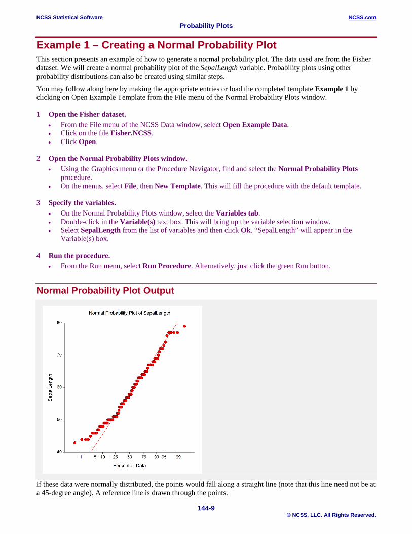
Example 1 – Creating a Normal Probability Plot This section presents an example of how to generate a normal probability plot. The data used are from the Fisher dataset. We will create a normal probability plot of the SepalLength variable. Probability plots using other probability distributions can also be created using similar steps.

You may follow along here by making the appropriate entries or load the completed template Example 1 by clicking on Open Example Template from the File menu of the Normal Probability Plots window.

1 Open the Fisher dataset. • From the File menu of the NCSS Data window, select Open Example Data. • Click on the file Fisher.NCSS. • Click Open.

2 Open the Normal Probability Plots window. • Using the Graphics menu or the Procedure Navigator, find and select the Normal Probability Plots

procedure. • On the menus, select File, then New Template. This will fill the procedure with the default template.

3 Specify the variables. • On the Normal Probability Plots window, select the Variables tab. • Double-click in the Variable(s) text box. This will bring up the variable selection window. • Select SepalLength from the list of variables and then click Ok. “SepalLength” will appear in the

Variable(s) box.

4 Run the procedure. • From the Run menu, select Run Procedure. Alternatively, just click the green Run button.

Normal Probability Plot Output

If these data were normally distributed, the points would fall along a straight line (note that this line need not be at a 45-degree angle). A reference line is drawn through the points.




Example 2 – Normal Probability Plot with Groups This section presents an example of how to generate a probability plot with three groups of data. The data used are from the Fisher dataset. We will create a probability plot of the SepalLength variable for each of the three varieties of iris. To run this example, take the following steps:

You may follow along here by making the appropriate entries or load the completed template Example 2 by clicking on Open Example Template from the File menu of the Normal Probability Plots window.


2 Open the Normal Probability Plots window. • Using the Graphics menu or the Procedure Navigator, find and select the Normal Probability Plots


3 Specify the variables. • On the Normal Probability Plots window, select the Variables tab. • Double-click in the Variable(s) text box. This will bring up the variable selection window. • Select SepalLength from the list of variables and then click Ok. “SepalLength” will appear in the

Variable(s) box. • Double-click in the Grouping Variable text box. This will bring up the variable selection window. • Select Iris from the list of variables and then click Ok. “Iris” will appear in the Group Variable box.


Normal Probability Plot Output

This is a normal probability plot of the SepalLength variable. We have separated the data according to iris variety. Note how well the data are modeled by the normal distribution.




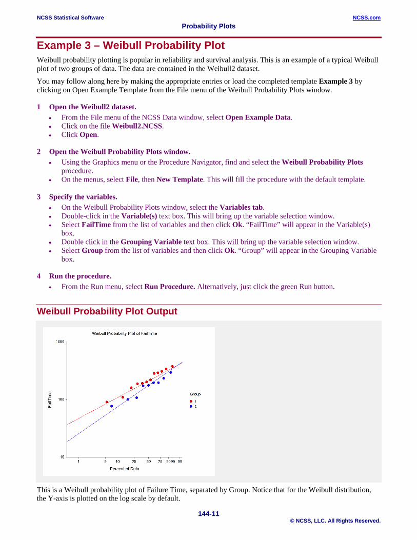
Example 3 – Weibull Probability Plot Weibull probability plotting is popular in reliability and survival analysis. This is an example of a typical Weibull plot of two groups of data. The data are contained in the Weibull2 dataset.

You may follow along here by making the appropriate entries or load the completed template Example 3 by clicking on Open Example Template from the File menu of the Weibull Probability Plots window.

1 Open the Weibull2 dataset. • From the File menu of the NCSS Data window, select Open Example Data. • Click on the file Weibull2.NCSS. • Click Open.

2 Open the Weibull Probability Plots window. • Using the Graphics menu or the Procedure Navigator, find and select the Weibull Probability Plots


3 Specify the variables. • On the Weibull Probability Plots window, select the Variables tab. • Double-click in the Variable(s) text box. This will bring up the variable selection window. • Select FailTime from the list of variables and then click Ok. “FailTime” will appear in the Variable(s)

box. • Double click in the Grouping Variable text box. This will bring up the variable selection window. • Select Group from the list of variables and then click Ok. “Group” will appear in the Grouping Variable

box.


Weibull Probability Plot Output

This is a Weibull probability plot of Failure Time, separated by Group. Notice that for the Weibull distribution, the Y-axis is plotted on the log scale by default.




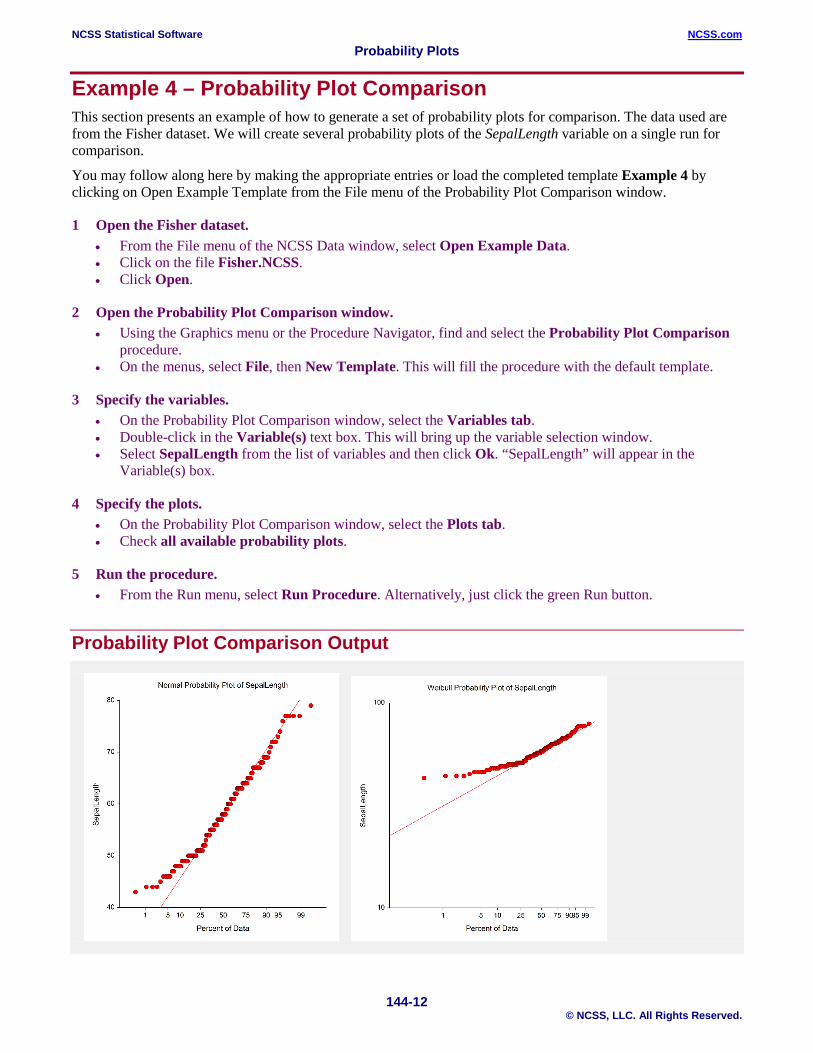
Example 4 – Probability Plot Comparison This section presents an example of how to generate a set of probability plots for comparison. The data used are from the Fisher dataset. We will create several probability plots of the SepalLength variable on a single run for comparison.

You may follow along here by making the appropriate entries or load the completed template Example 4 by clicking on Open Example Template from the File menu of the Probability Plot Comparison window.


2 Open the Probability Plot Comparison window. • Using the Graphics menu or the Procedure Navigator, find and select the Probability Plot Comparison


3 Specify the variables. • On the Probability Plot Comparison window, select the Variables tab. • Double-click in the Variable(s) text box. This will bring up the variable selection window. • Select SepalLength from the list of variables and then click Ok. “SepalLength” will appear in the

Variable(s) box.

4 Specify the plots. • On the Probability Plot Comparison window, select the Plots tab. • Check all available probability plots.


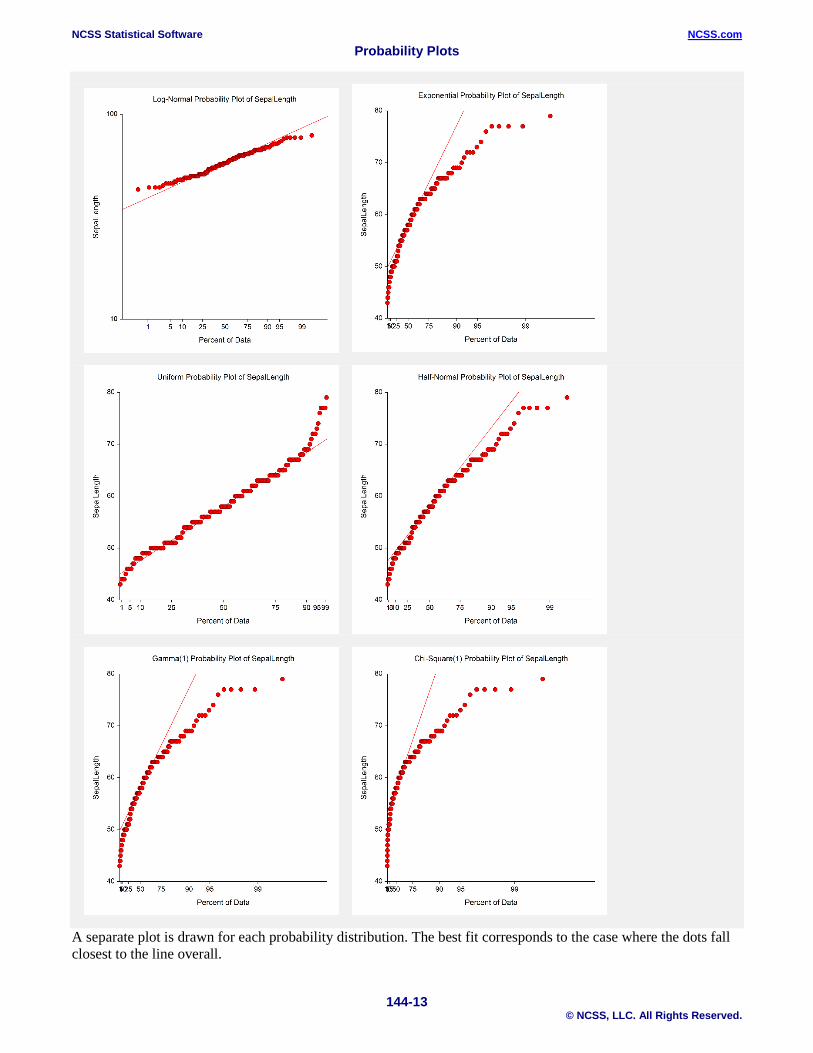
Probability Plot Comparison Output




A separate plot is drawn for each probability distribution. The best fit corresponds to the case where the dots fall closest to the line overall.


chapter 144 probability plots - statistical software ... · chapter 144 probability plots...

Documents