chapter 15 - mihaylo faculty websites - mihaylo faculty...
TRANSCRIPT

Chapter 15Multiple Regression
Learning Objectives
1. Understand how multiple regression analysis can be used to develop relationships involving one dependent variable and several independent variables.
2. Be able to interpret the coefficients in a multiple regression analysis.
3. Know the assumptions necessary to conduct statistical tests involving the hypothesized regression model.
4. Understand the role of computer packages in performing multiple regression analysis.
5. Be able to interpret and use computer output to develop the estimated regression equation.
6. Be able to determine how good a fit is provided by the estimated regression equation.
7. Be able to test for the significance of the regression equation.
8. Understand how multicollinearity affects multiple regression analysis.
9. Know how residual analysis can be used to make a judgement as to the appropriateness of the model, identify outliers, and determine which observations are influential.
10. Understand how logistic regression is used for regression analyses involving a binary dependent variable.
15 - 1© 2013 Cengage Learning. All Rights Reserved.
May not be scanned, copied or duplicated, or posted to a publicly accessible website, in whole or in part.

Chapter 15
Solutions:
1. a. b1 = .5906 is an estimate of the change in y corresponding to a 1 unit change in x1 when x2 is held constant.
b2 = .4980 is an estimate of the change in y corresponding to a 1 unit change in x2 when x1 is held constant.
b. = 29.1270 + .5906(180) + .4980(310) = 289.82
2. a. The estimated regression equation is
= 45.06 + 1.94x1
An estimate of y when x1 = 45 is
= 45.06 + 1.94(45) = 132.36
b. The estimated regression equation is
= 85.22 + 4.32x2
An estimate of y when x2 = 15 is
= 85.22 + 4.32(15) = 150.02
c. The estimated regression equation is
= -18.37 + 2.01x1 + 4.74x2
An estimate of y when x1 = 45 and x2 = 15 is
= -18.37 + 2.01(45) + 4.74(15) = 143.18
3. a. b1 = 3.8 is an estimate of the change in y corresponding to a 1 unit change in x1 when x2, x3, and x4 are held constant.
b2 = -2.3 is an estimate of the change in y corresponding to a 1 unit change in x2 when x1, x3, and x4 are held constant.
b3 = 7.6 is an estimate of the change in y corresponding to a 1 unit change in x3 when x1, x2, and x4 are held constant.
b4 = 2.7 is an estimate of the change in y corresponding to a 1 unit change in x4 when x1, x2, and x3 are held constant.
b. = 17.6 + 3.8(10) – 2.3(5) + 7.6(1) + 2.7(2) = 57.1
15 - © 2013 Cengage Learning. All Rights Reserved.
May not be scanned, copied or duplicated, or posted to a publicly accessible website, in whole or in part.

Multiple Regression
4. a. = 25 + 10(15) + 8(10) = 255; sales estimate: $255,000
b. Sales can be expected to increase by $10 for every dollar increase in inventory investment when advertising expenditure is held constant. Sales can be expected to increase by $8 for every dollar increase in advertising expenditure when inventory investment is held constant.
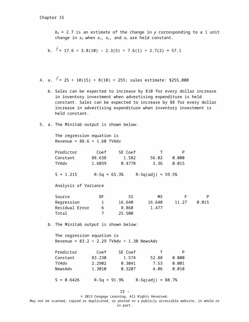
5. a. The Minitab output is shown below:
The regression equation isRevenue = 88.6 + 1.60 TVAdv
Predictor Coef SE Coef T PConstant 88.638 1.582 56.02 0.000TVAdv 1.6039 0.4778 3.36 0.015
S = 1.215 R-Sq = 65.3% R-Sq(adj) = 59.5%
Analysis of Variance
Source DF SS MS F PRegression 1 16.640 16.640 11.27 0.015Residual Error 6 8.860 1.477Total 7 25.500
b. The Minitab output is shown below:
The regression equation isRevenue = 83.2 + 2.29 TVAdv + 1.30 NewsAdv
Predictor Coef SE Coef T PConstant 83.230 1.574 52.88 0.000TVAdv 2.2902 0.3041 7.53 0.001NewsAdv 1.3010 0.3207 4.06 0.010
S = 0.6426 R-Sq = 91.9% R-Sq(adj) = 88.7%
Analysis of Variance
Source DF SS MS F PRegression 2 23.435 11.718 28.38 0.002Residual Error 5 2.065 0.413Total 7 25.500
c. No, it is 1.60 in part (a) and 2.29 above. In part (b) it represents the marginal change in revenue due to an increase in television advertising with newspaper advertising held constant.
d. Revenue = 83.2 + 2.29(3.5) + 1.30(1.8) = $93.56 or $93,560
15 - © 2013 Cengage Learning. All Rights Reserved.
May not be scanned, copied or duplicated, or posted to a publicly accessible website, in whole or in part.
Chapter 15
6. a. The Minitab output is shown below:
The regression equation isWin% = - 58.8 + 16.4 Yds/Att
Predictor Coef SE Coef T PConstant -58.77 26.18 -2.25 0.041Yds/Att 16.391 3.750 4.37 0.001
S = 15.8732 R-Sq = 57.7% R-Sq(adj) = 54.7%
Analysis of Variance
Source DF SS MS F PRegression 1 4814.3 4814.3 19.11 0.001Residual Error 14 3527.4 252.0Total 15 8341.7
Unusual Observations
Obs Yds/Att Win% Fit SE Fit Residual St Resid 14 6.50 81.30 47.77 4.24 33.53 2.19R
R denotes an observation with a large standardized residual.
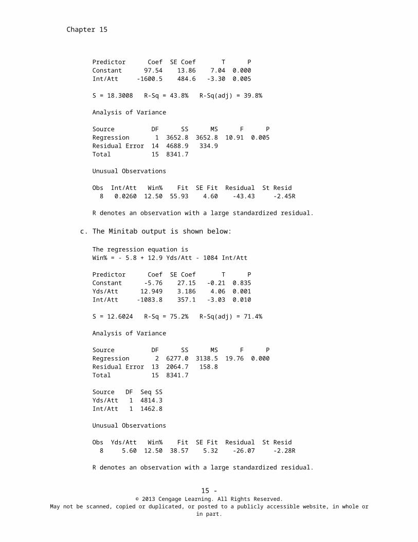
b. The Minitab output is shown below:
The regression equation isWin% = 97.5 - 1600 Int/Att
Predictor Coef SE Coef T PConstant 97.54 13.86 7.04 0.000Int/Att -1600.5 484.6 -3.30 0.005
S = 18.3008 R-Sq = 43.8% R-Sq(adj) = 39.8%
Analysis of Variance
Source DF SS MS F PRegression 1 3652.8 3652.8 10.91 0.005Residual Error 14 4688.9 334.9Total 15 8341.7
Unusual Observations
Obs Int/Att Win% Fit SE Fit Residual St Resid 8 0.0260 12.50 55.93 4.60 -43.43 -2.45R
R denotes an observation with a large standardized residual.
c. The Minitab output is shown below:
The regression equation isWin% = - 5.8 + 12.9 Yds/Att - 1084 Int/Att
Predictor Coef SE Coef T PConstant -5.76 27.15 -0.21 0.835Yds/Att 12.949 3.186 4.06 0.001Int/Att -1083.8 357.1 -3.03 0.010
S = 12.6024 R-Sq = 75.2% R-Sq(adj) = 71.4%
15 - © 2013 Cengage Learning. All Rights Reserved.
May not be scanned, copied or duplicated, or posted to a publicly accessible website, in whole or in part.

Multiple Regression
Analysis of Variance
Source DF SS MS F PRegression 2 6277.0 3138.5 19.76 0.000Residual Error 13 2064.7 158.8Total 15 8341.7
Source DF Seq SSYds/Att 1 4814.3Int/Att 1 1462.8
Unusual Observations
Obs Yds/Att Win% Fit SE Fit Residual St Resid 8 5.60 12.50 38.57 5.32 -26.07 -2.28R
R denotes an observation with a large standardized residual.
d. The predicted value of Win% for the Kansas City Chiefs is
Win% = - 5.8 + 12.9(6.2) – 1084(.036) = 35%
With 7 wins and 9 loses, the Kansas City Chiefs won 44% of the games they played. The predicted value is somewhat lower than the actual value.
7. a. The Minitab output is shown below:
The regression equation isPCW Rating = 66.1 + 0.170 Performance
Predictor Coef SE Coef T PConstant 66.062 3.793 17.42 0.000Performance 0.16989 0.05407 3.14 0.014
S = 2.59221 R-Sq = 55.2% R-Sq(adj) = 49.6%
Analysis of Variance
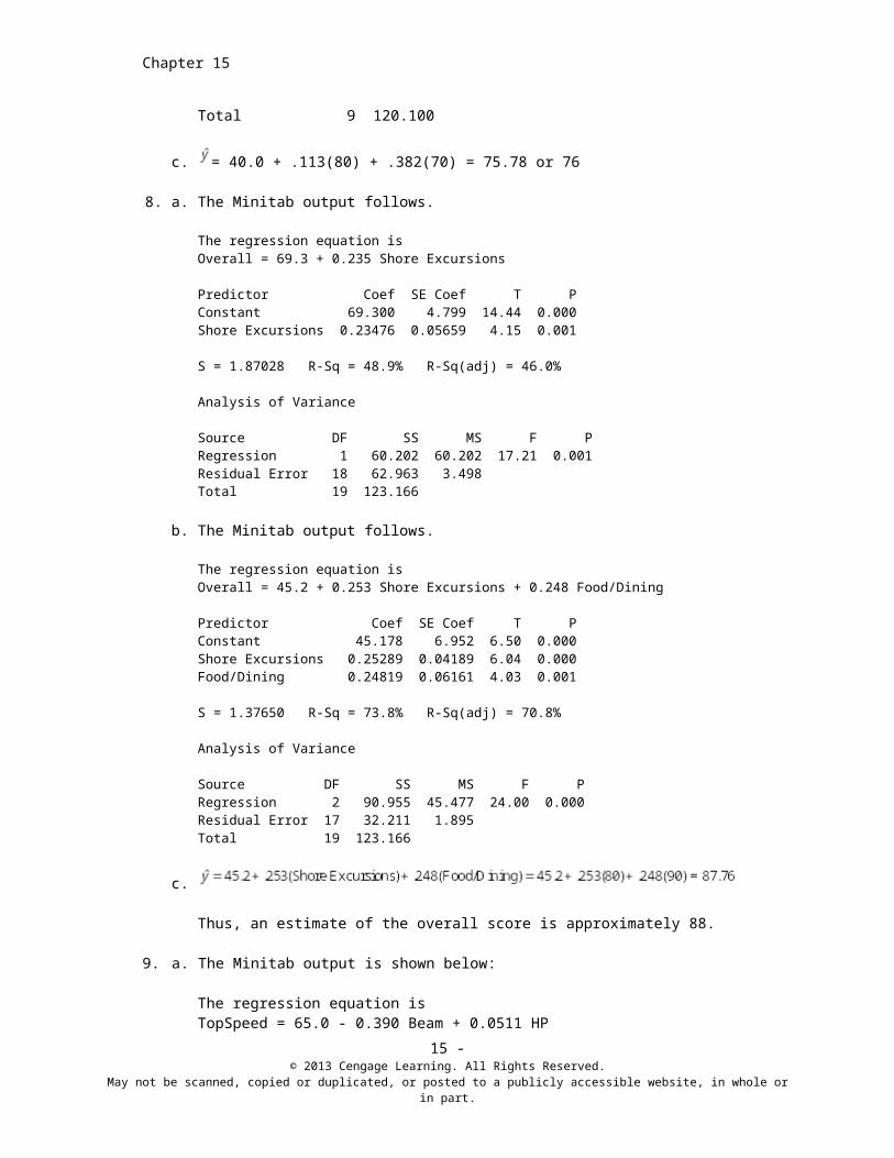
Source DF SS MS F PRegression 1 66.343 66.343 9.87 0.014Residual Error 8 53.757 6.720Total 9 120.100
b. The Minitab output is shown below:
The regression equation isPCW Rating = 40.0 + 0.113 Performance + 0.382 Features
Predictor Coef SE Coef T PConstant 39.982 7.855 5.09 0.001Performance 0.11338 0.03846 2.95 0.021Features 0.3820 0.1093 3.49 0.010
S = 1.67285 R-Sq = 83.7% R-Sq(adj) = 79.0%
15 - © 2013 Cengage Learning. All Rights Reserved.
May not be scanned, copied or duplicated, or posted to a publicly accessible website, in whole or in part.
Chapter 15
Analysis of Variance
Source DF SS MS F PRegression 2 100.511 50.255 17.96 0.002Residual Error 7 19.589 2.798Total 9 120.100
c. = 40.0 + .113(80) + .382(70) = 75.78 or 76
8. a. The Minitab output follows.
The regression equation isOverall = 69.3 + 0.235 Shore Excursions
Predictor Coef SE Coef T PConstant 69.300 4.799 14.44 0.000Shore Excursions 0.23476 0.05659 4.15 0.001
S = 1.87028 R-Sq = 48.9% R-Sq(adj) = 46.0%
Analysis of Variance
Source DF SS MS F PRegression 1 60.202 60.202 17.21 0.001Residual Error 18 62.963 3.498Total 19 123.166
b. The Minitab output follows.
The regression equation isOverall = 45.2 + 0.253 Shore Excursions + 0.248 Food/Dining
Predictor Coef SE Coef T PConstant 45.178 6.952 6.50 0.000Shore Excursions 0.25289 0.04189 6.04 0.000Food/Dining 0.24819 0.06161 4.03 0.001
S = 1.37650 R-Sq = 73.8% R-Sq(adj) = 70.8%
Analysis of Variance
Source DF SS MS F PRegression 2 90.955 45.477 24.00 0.000Residual Error 17 32.211 1.895Total 19 123.166
c.
Thus, an estimate of the overall score is approximately 88.
9. a. The Minitab output is shown below:
The regression equation isTopSpeed = 65.0 - 0.390 Beam + 0.0511 HP
Predictor Coef SE Coef T PConstant 64.966 9.009 7.21 0.000
15 - © 2013 Cengage Learning. All Rights Reserved.
May not be scanned, copied or duplicated, or posted to a publicly accessible website, in whole or in part.

Multiple Regression
Beam -0.38959 0.09579 -4.07 0.001HP 0.05106 0.01312 3.89 0.001
S = 1.59538 R-Sq = 59.7% R-Sq(adj) = 55.0%
Analysis of Variance
Source DF SS MS F PRegression 2 64.157 32.078 12.60 0.000Residual Error 17 43.269 2.545Total 19 107.426
b. = 64.966 - .38959 Beam + .05106 HP = 64.966 - .38959(85) + .05106(330) = 48.70
Thus, an estimate of the top speed for the Svfara SV609 is 48.7 mph.
10. a. The Minitab output follows.
The regression equation isR/IP = 0.676 - 0.284 SO/IP
Predictor Coef SE Coef T PConstant 0.67575 0.06307 10.71 0.000SO/IP -0.28385 0.07869 -3.61 0.002
S = 0.0602733 R-Sq = 42.0% R-Sq(adj) = 38.7%
Analysis of Variance
Source DF SS MS F PRegression 1 0.047263 0.047263 13.01 0.002Residual Error 18 0.065392 0.003633Total 19 0.112655
b. The Minitab output follows.
The regression equation isR/IP = 0.308 + 1.35 HR/IP
Predictor Coef SE Coef T PConstant 0.30805 0.06036 5.10 0.000HR/IP 1.3467 0.5407 2.49 0.023
S = 0.0682239 R-Sq = 25.6% R-Sq(adj) = 21.5%
Analysis of Variance
Source DF SS MS F PRegression 1 0.028874 0.028874 6.20 0.023Residual Error 18 0.083781 0.004655Total 19 0.112655
Unusual Observations
Obs HR/IP R/IP Fit SE Fit Residual St Resid 1 0.100 0.2900 0.4427 0.0159 -0.1527 -2.30R
R denotes an observation with a large standardized residual.
15 - © 2013 Cengage Learning. All Rights Reserved.
May not be scanned, copied or duplicated, or posted to a publicly accessible website, in whole or in part.
Chapter 15
c. The Minitab output follows.
The regression equation isR/IP = 0.537 - 0.248 SO/IP + 1.03 HR/IP
Predictor Coef SE Coef T PConstant 0.53651 0.08141 6.59 0.000SO/IP -0.24835 0.07181 -3.46 0.003HR/IP 1.0319 0.4359 2.37 0.030
S = 0.0537850 R-Sq = 56.3% R-Sq(adj) = 51.2%
Analysis of Variance
Source DF SS MS F PRegression 2 0.063477 0.031738 10.97 0.001Residual Error 17 0.049178 0.002893Total 19 0.112655
d. Using the estimated regression equation in part (c) we obtain
R/IP = 0.537 - 0.248 SO/IP + 1.03 HR/IPR/IP = 0.537 - 0.248(.91)+ 1.03(.16)= .48
The predicted value for R/IP was less than the actual value.
e. This suggestion does not make sense. If a pitcher gives up more runs per inning pitched this pitcher’s earned run average also has to increase. For these data the sample correlation coefficient between ERA and R/IP is .964. The following Minitab output shows the results for part (c) using ERA as the dependent variable.
The regression equation isERA = 3.88 + 12.0 HR/IP - 1.84 SO/IP
Predictor Coef SE Coef T PConstant 3.8781 0.6466 6.00 0.000HR/IP 11.993 3.462 3.46 0.003SO/IP -1.8428 0.5703 -3.23 0.005
S = 0.427204 R-Sq = 62.5% R-Sq(adj) = 58.1%
Analysis of Variance
Source DF SS MS F PRegression 2 5.1739 2.5870 14.17 0.000Residual Error 17 3.1025 0.1825Total 19 8.2765
11. a. SSE = SST - SSR = 6,724.125 - 6,216.375 = 507.75
b.
c.d. The estimated regression equation provided an excellent fit.
15 - © 2013 Cengage Learning. All Rights Reserved.
May not be scanned, copied or duplicated, or posted to a publicly accessible website, in whole or in part.

Multiple Regression
12. a.
b.
c. Yes; after adjusting for the number of independent variables in the model, we see that 90.5% of the variability in y has been accounted for.
13. a.
b.
c. The estimated regression equation provided an excellent fit.
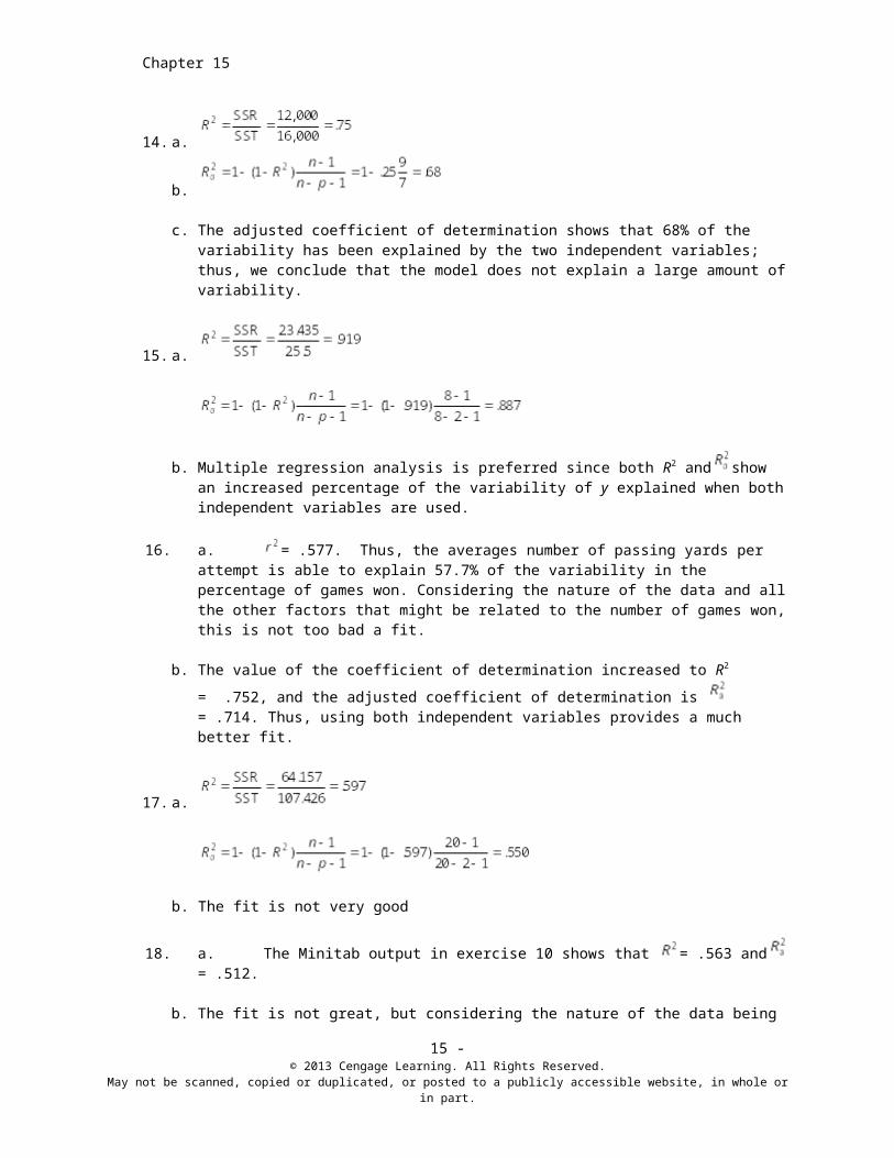
14. a.
b.
c. The adjusted coefficient of determination shows that 68% of the variability has been explained by the two independent variables; thus, we conclude that the model does not explain a large amount of variability.
15. a.
b. Multiple regression analysis is preferred since both R2 and show an increased percentage of the variability of y explained when both independent variables are used.
16. a. = .577. Thus, the averages number of passing yards per attempt is able to explain 57.7% of the variability in the percentage of games won. Considering the nature of the data and all the other factors that might be related to the number of games won, this is not too bad a fit.
b. The value of the coefficient of determination increased to R2 = .752, and the adjusted coefficient of
determination is = .714. Thus, using both independent variables provides a much better fit.
17. a.
15 - © 2013 Cengage Learning. All Rights Reserved.
May not be scanned, copied or duplicated, or posted to a publicly accessible website, in whole or in part.

Chapter 15
b. The fit is not very good
18. a. The Minitab output in exercise 10 shows that = .563 and = .512.
b. The fit is not great, but considering the nature of the data being able to explain slightly more than 50% of the variability in the number of runs given up per inning pitched using just two independent variables is not too bad.
c. The Minitab output using ERA as the dependent variable follows.
The regression equation isERA = 3.88 + 12.0 HR/IP - 1.84 SO/IP
Predictor Coef SE Coef T PConstant 3.8781 0.6466 6.00 0.000HR/IP 11.993 3.462 3.46 0.003SO/IP -1.8428 0.5703 -3.23 0.005
S = 0.427204 R-Sq = 62.5% R-Sq(adj) = 58.1%
Analysis of Variance
Source DF SS MS F PRegression 2 5.1739 2.5870 14.17 0.000Residual Error 17 3.1025 0.1825Total 19 8.2765
The Minitab output shows that = .625 and = .581
Approximately 60% of the variability in the ERA can be explained by the linear effect of HR/IP and SO/IP. This is not too bad considering the complexity of predicting pithing performance.
19. a. MSR = SSR/p = 6,216.375/2 = 3,108.188
b. F = MSR/MSE = 3,108.188/72.536 = 42.85
Using F table (2 degrees of freedom numerator and 7 denominator), p-value is less than .01
Actual p-value = .0001
Because p-value = .05, the overall model is significant.
c. t = .5906/.0813 = 7.26
Using t table (7 degrees of freedom), area in tail is less than .005; p-value is less than .01
Actual p-value = .0002
15 - © 2013 Cengage Learning. All Rights Reserved.
May not be scanned, copied or duplicated, or posted to a publicly accessible website, in whole or in part.

Multiple Regression
Because p-value is significant.
d. t = .4980/.0567 = 8.78
Using t table (7 degrees of freedom), area in tail is less than .005; p-value is less than .01
Actual p-value = .0001
Because p-value is significant.
20. A portion of the Minitab output is shown below.
The regression equation isY = - 18.4 + 2.01 X1 + 4.74 X2
Predictor Coef SE Coef T PConstant -18.37 17.97 -1.02 0.341X1 2.0102 0.2471 8.13 0.000X2 4.7378 0.9484 5.00 0.002
S = 12.71 R-Sq = 92.6% R-Sq(adj) = 90.4%
Analysis of Variance
Source DF SS MS F PRegression 2 14052.2 7026.1 43.50 0.000Residual Error 7 1130.7 161.5Total 9 15182.9
a. Since the p-value corresponding to F = 43.50 is .000 < = .05, we reject H0: = = 0; there is a significant relationship.
b. Since the p-value corresponding to t = 8.13 is .000 < = .05, we reject H0: = 0; is significant.
c. Since the p-value corresponding to t = 5.00 is .002 < = .05, we reject H0: = 0; is significant.
21. a. In the two independent variable case the coefficient of x1 represents the expected change in y corresponding to a one unit increase in x1 when x2 is held constant. In the single independent variable case the coefficient of x1 represents the expected change in y corresponding to a one unit increase in x1.
b. Yes. If x1 and x2 are correlated one would expect a change in x1 to be accompanied by a change in x2.
22. a. SSE = SST - SSR = 16000 - 12000 = 4000
15 - © 2013 Cengage Learning. All Rights Reserved.
May not be scanned, copied or duplicated, or posted to a publicly accessible website, in whole or in part.
Chapter 15
b. F = MSR/MSE = 6000/571.43 = 10.50
Using F table (2 degrees of freedom numerator and 7 denominator), p-value is less than .01
Actual p-value = .008
Because p-value we reject H0. There is a significant relationship among the variables.
23. a. F = 28.38
Using F table (2 degrees of freedom numerator and 5 denominator), p-value is less than .01
Actual p-value = .002
Because p-value there is a significant relationship.
b. t = 7.53
Using t table (5 degrees of freedom), area in tail is less than .005; p-value is less than .01
Actual p-value = .001
Because p-value is significant and x1 should not be dropped from the model.
c. t = 4.06
Actual p-value = .010
Because p-value is significant and x2 should not be dropped from the model.
24. a. The Minitab output is shown below:
The regression equation isSalary = - 0.682 + 0.0498 Revenue + 0.0147 %Wins
Predictor Coef SE Coef T PConstant -0.6820 0.5044 -1.35 0.185Revenue 0.04983 0.01345 3.70 0.001%Wins 0.014683 0.006291 2.33 0.025
S = 0.328622 R-Sq = 31.9% R-Sq(adj) = 28.1%
Analysis of Variance
Source DF SS MS F PRegression 2 1.8188 0.9094 8.42 0.001Residual Error 36 3.8877 0.1080Total 38 5.7065
b. Because the p-value = .001< = .05, there is a significant relationship.
15 - © 2013 Cengage Learning. All Rights Reserved.
May not be scanned, copied or duplicated, or posted to a publicly accessible website, in whole or in part.

Multiple Regression
c. For Revenue: Because the p-value = .001 < = .05, Revenue is significant.
For %Wins: Because the p-value = .025 < = .05, %Wins is significant.25. a. The Minitab output follows.
The regression equation isOverall = 35.6 + 0.110 Itineraries/Schedule + 0.245 Shore Excursions + 0.247 Food/Dining
Predictor Coef SE Coef T PConstant 35.62 13.23 2.69 0.016Itineraries/Schedule 0.1105 0.1297 0.85 0.407Shore Excursions 0.24454 0.04336 5.64 0.000Food/Dining 0.24736 0.06212 3.98 0.001
S = 1.38775 R-Sq = 75.0% R-Sq(adj) = 70.3%
Analysis of Variance
Source DF SS MS F PRegression 3 92.352 30.784 15.98 0.000Residual Error 16 30.813 1.926Total 19 123.166
Total 19 123.166
b. Because the p-value corresponding to F = 15.98, 0.000, is less than .05, the level of significance, overall there is a significant relationship.
c. Because the p-value for Itineraries/Schedule (.407) is greater than the level of significance (.05), Itineraries/Schedule is not significant. Shore Excursions (p-value = .000) and Food/Dining (p-value = .001) are both significant because the p-value for each of these independent variables is less than the level of significance (.05).
d. After removing Itineraries/Schedule from the model, we obtained the following Minitab output.
The regression equation isOverall = 45.2 + 0.253 Shore Excursions + 0.248 Food/Dining
Predictor Coef SE Coef T PConstant 45.178 6.952 6.50 0.000Shore Excursions 0.25289 0.04189 6.04 0.000Food/Dining 0.24819 0.06161 4.03 0.001
S = 1.37650 R-Sq = 73.8% R-Sq(adj) = 70.8%
Analysis of Variance
Source DF SS MS F PRegression 2 90.955 45.477 24.00 0.000Residual Error 17 32.211 1.895Total 19 123.166
With Itineraries/Schedule in the model, the R2 was .750, while the R2 after Itineraries/Schedule was removed from the model was .738. Removing Itineraries/Schedule from the model resulted in almost no loss in the model’s ability to explain variability in the Overall Score.
15 - © 2013 Cengage Learning. All Rights Reserved.
May not be scanned, copied or duplicated, or posted to a publicly accessible website, in whole or in part.

Chapter 15
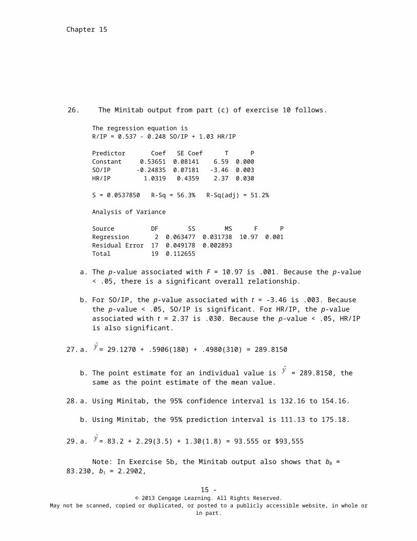
26. The Minitab output from part (c) of exercise 10 follows.
The regression equation isR/IP = 0.537 - 0.248 SO/IP + 1.03 HR/IP
Predictor Coef SE Coef T PConstant 0.53651 0.08141 6.59 0.000SO/IP -0.24835 0.07181 -3.46 0.003HR/IP 1.0319 0.4359 2.37 0.030
S = 0.0537850 R-Sq = 56.3% R-Sq(adj) = 51.2%
Analysis of Variance
Source DF SS MS F PRegression 2 0.063477 0.031738 10.97 0.001Residual Error 17 0.049178 0.002893Total 19 0.112655
a. The p-value associated with F = 10.97 is .001. Because the p-value < .05, there is a significant overall relationship.
b. For SO/IP, the p-value associated with t = -3.46 is .003. Because the p-value < .05, SO/IP is significant. For HR/IP, the p-value associated with t = 2.37 is .030. Because the p-value < .05, HR/IP is also significant.
27. a. = 29.1270 + .5906(180) + .4980(310) = 289.8150
b. The point estimate for an individual value is = 289.8150, the same as the point estimate of the mean value.
28. a. Using Minitab, the 95% confidence interval is 132.16 to 154.16.
b. Using Minitab, the 95% prediction interval is 111.13 to 175.18.
29. a. = 83.2 + 2.29(3.5) + 1.30(1.8) = 93.555 or $93,555
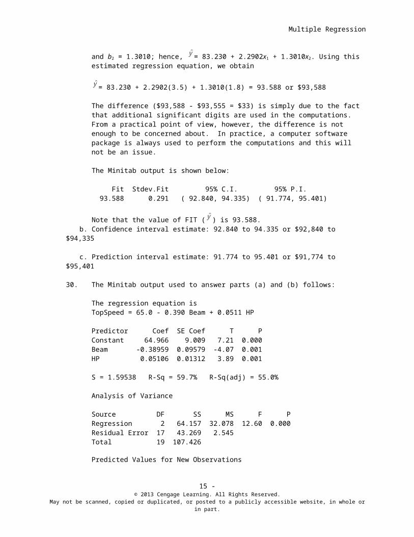
Note: In Exercise 5b, the Minitab output also shows that b0 = 83.230, b1 = 2.2902,
and b2 = 1.3010; hence, = 83.230 + 2.2902x1 + 1.3010x2. Using this estimated regression equation, we obtain
= 83.230 + 2.2902(3.5) + 1.3010(1.8) = 93.588 or $93,588
The difference ($93,588 - $93,555 = $33) is simply due to the fact that additional significant digits are used in the computations. From a practical point of view, however, the difference is not enough to be concerned about. In practice, a computer software package is always used to perform the computations and this will not be an issue.
The Minitab output is shown below:
15 - © 2013 Cengage Learning. All Rights Reserved.
May not be scanned, copied or duplicated, or posted to a publicly accessible website, in whole or in part.

Multiple Regression
Fit Stdev.Fit 95% C.I. 95% P.I. 93.588 0.291 ( 92.840, 94.335) ( 91.774, 95.401)
Note that the value of FIT ( ) is 93.588.b. Confidence interval estimate: 92.840 to 94.335 or $92,840 to $94,335
c. Prediction interval estimate: 91.774 to 95.401 or $91,774 to $95,401
30. The Minitab output used to answer parts (a) and (b) follows:
The regression equation isTopSpeed = 65.0 - 0.390 Beam + 0.0511 HP
Predictor Coef SE Coef T PConstant 64.966 9.009 7.21 0.000Beam -0.38959 0.09579 -4.07 0.001HP 0.05106 0.01312 3.89 0.001
S = 1.59538 R-Sq = 59.7% R-Sq(adj) = 55.0%
Analysis of Variance
Source DF SS MS F PRegression 2 64.157 32.078 12.60 0.000Residual Error 17 43.269 2.545Total 19 107.426
Predicted Values for New Observations
NewObs Fit SE Fit 95% CI 95% PI 1 48.702 0.921 (46.758, 50.646) (44.815, 52.589)
a. The 95% confidence interval is 46.758 to 50.646.
b. The 95% prediction interval for the Svfara SV609 is 44.815 to 52.589.
31. a. A portion of the Minitab output follows.
The regression equation isSatisfaction Electronic Trades = - 0.783 + 0.558 Trade Price + 0.734 Speed of Execution
Predictor Coef SE Coef T PConstant -0.7835 0.9423 -0.83 0.423Trade Price 0.5580 0.2332 2.39 0.036Speed of Execution 0.7342 0.1557 4.71 0.001
S = 0.410845 R-Sq = 68.3% R-Sq(adj) = 62.5%
Analysis of Variance
Source DF SS MS F PRegression 2 3.9954 1.9977 11.84 0.002Residual Error 11 1.8567 0.1688Total 13 5.8521
15 - © 2013 Cengage Learning. All Rights Reserved.
May not be scanned, copied or duplicated, or posted to a publicly accessible website, in whole or in part.

Chapter 15
b. Satisfaction Electronic Trades = - 0.783 + 0.558(3)+ 0.734(3) = 3.093
c./d.A portion of the Minitab output follows.
Predicted Values for New Observations
New Obs Fit SE Fit 95% CI 95% PI 1 3.093 0.111 (2.848, 3.338) (2.156, 4.030)
For part (c) the 95% confidence interval is 2.848 to 3.338
For part (d) the 95% prediction interval is 2.156 to 4.030; but, because the highest possible rating is 4, the upper end of the prediction interval is treated as 4.
32. a. E(y) = + x1 + x2 where
x2 = 0 if level 1 and 1 if level 2
b. E(y) = + x1 + (0) = + x1
c. E(y) = + x1 + (1) = + x1 +
d. = E(y | level 2) - E(y | level 1)
is the change in E(y) for a 1 unit change in x1 holding x2 constant.
33. a. two
b. E(y) = + x1 + x2 + x3 where
x2 x3 Level0 0 11 0 20 1 3
c. E(y | level 1) = + x1 + (0) + (0) = + x1
E(y | level 2) = + x1 + (1) + (0) = + x1 +
E(y | level 3) = + x1 + (0) + (0) = + x1 +
= E(y | level 2) - E(y | level 1)
= E(y | level 3) - E(y | level 1)
is the change in E(y) for a 1 unit change in x1 holding x2 and x3 constant.
34. a. $15,300
b. Estimate of sales = 10.1 - 4.2(2) + 6.8(8) + 15.3(0) = 56.1 or $56,100
c. Estimate of sales = 10.1 - 4.2(1) + 6.8(3) + 15.3(1) = 41.6 or $41,600
15 - © 2013 Cengage Learning. All Rights Reserved.
May not be scanned, copied or duplicated, or posted to a publicly accessible website, in whole or in part.

Multiple Regression
35. a. Let Type = 0 if a mechanical repair Type = 1 if an electrical repair
The Minitab output is shown below:
The regression equation isTime = 3.45 + 0.617 Type
Predictor Coef SE Coef T PConstant 3.4500 0.5467 6.31 0.000Type 0.6167 0.7058 0.87 0.408
S = 1.093 R-Sq = 8.7% R-Sq(adj) = 0.0%
Analysis of Variance
Source DF SS MS F PRegression 1 0.913 0.913 0.76 0.408Residual Error 8 9.563 1.195Total 9 10.476
b. The estimated regression equation did not provide a good fit. In fact, the p-value of .408 shows that the relationship is not significant for any reasonable value of .
c. Person = 0 if Bob Jones performed the service and Person = 1 if Dave Newton performed the service. The Minitab output is shown below:
The regression equation isTime = 4.62 - 1.60 Person
Predictor Coef SE Coef T PConstant 4.6200 0.3192 14.47 0.000Person -1.6000 0.4514 -3.54 0.008
S = 0.7138 R-Sq = 61.1% R-Sq(adj) = 56.2%
Analysis of Variance
Source DF SS MS F PRegression 1 6.4000 6.4000 12.56 0.008Residual Error 8 4.0760 0.5095Total 9 10.4760
d. We see that 61.1% of the variability in repair time has been explained by the repair person that performed the service; an acceptable, but not good, fit.
15 - © 2013 Cengage Learning. All Rights Reserved.
May not be scanned, copied or duplicated, or posted to a publicly accessible website, in whole or in part.
Chapter 15
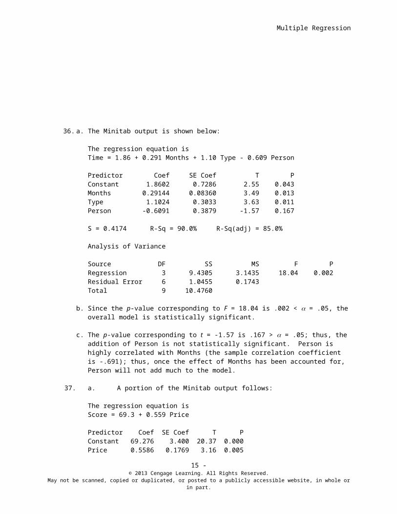
36. a. The Minitab output is shown below:
The regression equation isTime = 1.86 + 0.291 Months + 1.10 Type - 0.609 Person
Predictor Coef SE Coef T PConstant 1.8602 0.7286 2.55 0.043Months 0.29144 0.08360 3.49 0.013Type 1.1024 0.3033 3.63 0.011Person -0.6091 0.3879 -1.57 0.167
S = 0.4174 R-Sq = 90.0% R-Sq(adj) = 85.0%
Analysis of Variance
Source DF SS MS F PRegression 3 9.4305 3.1435 18.04 0.002Residual Error 6 1.0455 0.1743Total 9 10.4760
b. Since the p-value corresponding to F = 18.04 is .002 < = .05, the overall model is statistically significant.
c. The p-value corresponding to t = -1.57 is .167 > = .05; thus, the addition of Person is not statistically significant. Person is highly correlated with Months (the sample correlation coefficient is -.691); thus, once the effect of Months has been accounted for, Person will not add much to the model.
37. a. A portion of the Minitab output follows:
The regression equation isScore = 69.3 + 0.559 Price
Predictor Coef SE Coef T PConstant 69.276 3.400 20.37 0.000Price 0.5586 0.1769 3.16 0.005
S = 3.02575 R-Sq = 34.4% R-Sq(adj) = 31.0%
Analysis of Variance
Source DF SS MS F PRegression 1 91.290 91.290 9.97 0.005Residual Error 19 173.948 9.155Total 20 265.238
b. Because the p-value = .005 < α = .05, there is a significant relationship.
c. Let Type_Italian = 1 if the restaurant is an Italian restaurant; 0 otherwise
15 - © 2013 Cengage Learning. All Rights Reserved.
May not be scanned, copied or duplicated, or posted to a publicly accessible website, in whole or in part.
Multiple Regression
d. A portion of the Minitab output follows:
The regression equation isScore = 67.4 + 0.573 Price + 3.04 Type_Italian
Predictor Coef SE Coef T PConstant 67.405 3.053 22.07 0.000Price 0.5734 0.1546 3.71 0.002Type_Italian 3.038 1.155 2.63 0.017
S = 2.64219 R-Sq = 52.6% R-Sq(adj) = 47.4%
Analysis of Variance
Source DF SS MS F PRegression 2 139.577 69.789 10.00 0.001Residual Error 18 125.661 6.981Total 20 265.238
e. For the Type_Italian dummy variable, the p-value = .017 < α = .05; thus, type of restaurant is a significant factor in overall customer satisfaction.
f. The estimated regression equation computed in part (d) is = 67.4 + .573(Price) + 3.04(Type_Italian).
For a seafood/steakhouse Type_Italian = 0 and the estimated score is = 67.4 + .573(20) + 3.04(0) = 79.86
For an Italian restaurant Type_Italian = 1 and the estimated score is = 67.4 + .573(20) + 3.04(1) = 82.90
Thus, the satisfaction score increases by 3.04 points.
38. a. The Minitab output is shown below:
The regression equation isRisk = - 91.8 + 1.08 Age + 0.252 Pressure + 8.74 Smoker
Predictor Coef SE Coef T PConstant -91.76 15.22 -6.03 0.000Age 1.0767 0.1660 6.49 0.000Pressure 0.25181 0.04523 5.57 0.000Smoker 8.740 3.001 2.91 0.010
S = 5.757 R-Sq = 87.3% R-Sq(adj) = 85.0%
Analysis of Variance
Source DF SS MS F PRegression 3 3660.7 1220.2 36.82 0.000
15 - © 2013 Cengage Learning. All Rights Reserved.
May not be scanned, copied or duplicated, or posted to a publicly accessible website, in whole or in part.

Chapter 15
Residual Error 16 530.2 33.1Total 19 4190.9
b. Since the p-value corresponding to t = 2.91 is .010 < = .05, smoking is a significant factor.
c. Using Minitab, the point estimate is 34.27; the 95% prediction interval is 21.35 to 47.18. Thus, the probability of a stroke (.2135 to .4718 at the 95% confidence level) appears to be quite high. The physician would probably recommend that Art quit smoking and begin some type of treatment designed to reduce his blood pressure.
39. a. The Minitab output is shown below:
The regression equation isY = 0.20 + 2.60 X
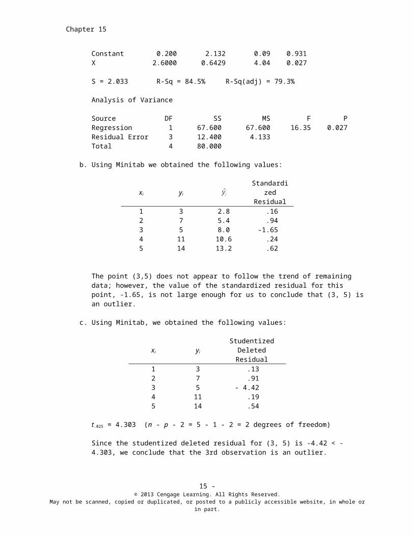
Predictor Coef SE Coef T PConstant 0.200 2.132 0.09 0.931X 2.6000 0.6429 4.04 0.027
S = 2.033 R-Sq = 84.5% R-Sq(adj) = 79.3%
Analysis of Variance
Source DF SS MS F PRegression 1 67.600 67.600 16.35 0.027Residual Error 3 12.400 4.133Total 4 80.000
b. Using Minitab we obtained the following values:
xi yi
Standardized Residual
1 3 2.8 .162 7 5.4 .943 5 8.0 -1.654 11 10.6 .245 14 13.2 .62
The point (3,5) does not appear to follow the trend of remaining data; however, the value of the standardized residual for this point, -1.65, is not large enough for us to conclude that (3, 5) is an outlier.
c. Using Minitab, we obtained the following values:
xi yi
StudentizedDeleted Residual
1 3 .132 7 .913 5 - 4.424 11 .195 14 .54
t.025 = 4.303 (n - p - 2 = 5 - 1 - 2 = 2 degrees of freedom)
15 - © 2013 Cengage Learning. All Rights Reserved.
May not be scanned, copied or duplicated, or posted to a publicly accessible website, in whole or in part.

Multiple Regression
Since the studentized deleted residual for (3, 5) is -4.42 < -4.303, we conclude that the 3rd observation is an outlier.
40. a. The Minitab output is shown below:
The regression equation isY = -53.3 + 3.11 X
Predicator Coef SE Coef T pConstant -53.280 5.786 -9.21 0.003X 3.1100 0.2016 15.43 0.001
S = 2.851 R-sq = 98.8% R-sq (adj) = 98.3%
Analysis of Variance
SOURCE DF SS MS F pRegression 1 1934.4 1934.4 238.03 0.001Residual Error 3 24.4 8.1Total 4 1598.8
b. Using the Minitab we obtained the following values:
xi yi
StudentizedDeleted Residual
22 12 -1.9424 21 -.1226 31 1.7928 35 .4040 70 -1.90
t.025 = 4.303 (n - p - 2 = 5 - 1 - 2 = 2 degrees of freedom)
Since none of the studentized deleted residuals are less than -4.303 or greater than 4.303, none of the observations can be classified as an outlier.
c. Using Minitab we obtained the following values:
xi yi hi
22 12 .3824 21 .2826 31 .2228 35 .2040 70 .92
The critical value is
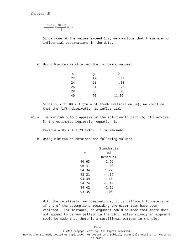
Since none of the values exceed 1.2, we conclude that there are no influential observations in the data.
15 - © 2013 Cengage Learning. All Rights Reserved.
May not be scanned, copied or duplicated, or posted to a publicly accessible website, in whole or in part.

Chapter 15
d. Using Minitab we obtained the following values:
xi yi Di
22 12 .6024 21 .0026 31 .2628 35 .0340 70 11.09
Since D5 = 11.09 > 1 (rule of thumb critical value), we conclude that the fifth observation is influential.
41. a. The Minitab output appears in the solution to part (b) of Exercise 5; the estimated regression equation is:
Revenue = 83.2 + 2.29 TVAdv + 1.30 NewsAdv
b. Using Minitab we obtained the following values:
Standardized Residual
96.63 -1.6290.41 -1.0894.34 1.2292.21 - .3794.39 1.1094.24 - .4094.42 -1.1293.35 1.08
With the relatively few observations, it is difficult to determine if any of the assumptions regarding the error term have been violated. For instance, an argument could be made that there does not appear to be any pattern in the plot; alternatively an argument could be made that there is a curvilinear pattern in the plot.
c. The values of the standardized residuals are greater than -2 and less than +2; thus, using test, there are no outliers. As a further check for outliers, we used Minitab to compute the following studentized deleted residuals:
ObservationStudentized
Deleted Residual1 -2.112 -1.103 1.314 - .335 1.136 - .367 -1.168 1.10
15 - © 2013 Cengage Learning. All Rights Reserved.
May not be scanned, copied or duplicated, or posted to a publicly accessible website, in whole or in part.
Multiple Regression
t.025 = 2.776 (n - p - 2 = 8 - 2 - 2 = 4 degrees of freedom)
Since none of the studentized deleted residuals is less than -2.776 or greater than 2.776, we conclude that there are no outliers in the data.
d. Using Minitab we obtained the following values:
Observation hi Di
1 .63 1.522 .65 .703 .30 .224 .23 .015 .26 .146 .14 .017 .66 .818 .13 .06
The critical value for leverage is
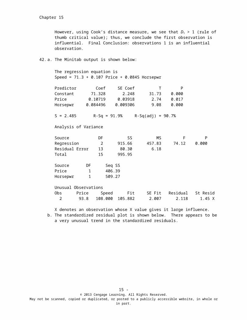
Since none of the values exceed 1.125, we conclude that there are no influential observations. However, using Cook’s distance measure, we see that D1 > 1 (rule of thumb critical value); thus, we conclude the first observation is influential. Final Conclusion: observations 1 is an influential observation.
42. a. The Minitab output is shown below:
The regression equation isSpeed = 71.3 + 0.107 Price + 0.0845 Horsepwr
Predictor Coef SE Coef T PConstant 71.328 2.248 31.73 0.000Price 0.10719 0.03918 2.74 0.017Horsepwr 0.084496 0.009306 9.08 0.000
S = 2.485 R-Sq = 91.9% R-Sq(adj) = 90.7%
Analysis of Variance
Source DF SS MS F PRegression 2 915.66 457.83 74.12 0.000Residual Error 13 80.30 6.18Total 15 995.95
Source DF Seq SSPrice 1 406.39Horsepwr 1 509.27
Unusual Observations
15 - © 2013 Cengage Learning. All Rights Reserved.
May not be scanned, copied or duplicated, or posted to a publicly accessible website, in whole or in part.

Chapter 15
Obs Price Speed Fit SE Fit Residual St Resid 2 93.8 108.000 105.882 2.007 2.118 1.45 X
X denotes an observation whose X value gives it large influence.b. The standardized residual plot is shown below. There appears to be a very unusual trend in the
standardized residuals.
c. The Minitab output shown in part (a) did not identify any observations with a large standardized residual; thus, there does not appear to be any outliers in the data.
d. The Minitab output shown in part (a) identifies observation 2 as an influential observation.
43. a. The Minitab output is shown below:
The regression equation isScoring Avg. = 58.1 - 10.7 Greens in Reg. + 11.7 Putting Avg.
Predictor Coef SE Coef T PConstant 58.090 6.053 9.60 0.000Greens in Reg. -10.736 3.016 -3.56 0.001Putting Avg. 11.707 2.899 4.04 0.000
S = 0.428970 R-Sq = 58.3% R-Sq(adj) = 55.2%
Analysis of Variance
Source DF SS MS F PRegression 2 6.9351 3.4675 18.84 0.000Residual Error 27 4.9684 0.1840Total 29 11.9035
Unusual Observations
Greens in ScoringObs Reg. Avg. Fit SE Fit Residual St Resid 1 0.772 69.3300 70.2887 0.2403 -0.9587 -2.70RX
15 - © 2013 Cengage Learning. All Rights Reserved.
May not be scanned, copied or duplicated, or posted to a publicly accessible website, in whole or in part.

Multiple Regression
14 0.631 71.8000 72.0366 0.2478 -0.2366 -0.68 X 30 0.728 72.1300 70.8781 0.1410 1.2519 3.09R
R denotes an observation with a large standardized residual.X denotes an observation whose X value gives it large influence.
b. The standardized residual plot is shown below:
The standardized residual plot does not support the assumption about . There are three unusual
observations and the variance of the residuals appears to be increasing for larger values of .
c. The Minitab output in part (a) identified two outliers: observations 1 and 30. Observation 1 corresponds to Annika Sorenstam; her scoring average was much lower than the other players. Observation 30 corresponds to Karine Icher; although her performance in terms of greens in regulation and putting average was very good, her scoring average was much higher than most of the other players.
d. The Minitab output in part (a) identified two influential observations: observations 1 and 14. Observation 1 corresponds to Annika Sorenstam and observation 14 corresponds to Soo-Yun Kang.
44. a.
b. It is an estimate of the probability that a customer that does not have a Simmons credit card will make a purchase.
c. A portion of the Minitab binary logistic regression output follows:
Logistic Regression Table Odds 95% CI
Predictor Coef SE Coef Z P Ratio Lower UpperConstant -0.9445 0.3150 -3.00 0.003Card 1.0245 0.4235 2.42 0.016 2.79 1.21 6.39
15 - © 2013 Cengage Learning. All Rights Reserved.
May not be scanned, copied or duplicated, or posted to a publicly accessible website, in whole or in part.
Chapter 15
Log-Likelihood = -64.265
Test that all slopes are zero: G = 6.072, DF = 1, P-Value = 0.014
Thus, the estimated logit is -0.9445 + 1.0245x
d. For customers that do not have a Simmons credit card (x = 0)
-0.9445 + 1.245(0) = 0.9445
and
For customers that have a Simmons credit card (x = 1)
-0.9445 + 1.245(1) = 0.0800
and
e. Using the Minitab output shown in part (c), the estimated odds ratio is 2.79. We can conclude that the estimated odds of making a purchase for customers who have a Simmons credit card are 2.79 times greater than the estimated odds of making a purchase for customers that do not have a Simmons credit card.
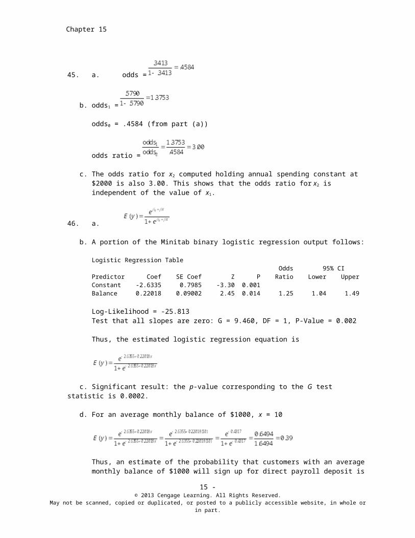
45. a. odds =
b. odds1 =
odds0 = .4584 (from part (a))
odds ratio =
c. The odds ratio for x2 computed holding annual spending constant at $2000 is also 3.00. This shows that the odds ratio for x2 is independent of the value of x1.
46. a.
b. A portion of the Minitab binary logistic regression output follows:
15 - © 2013 Cengage Learning. All Rights Reserved.
May not be scanned, copied or duplicated, or posted to a publicly accessible website, in whole or in part.

Multiple Regression
Logistic Regression Table Odds 95% CIPredictor Coef SE Coef Z P Ratio Lower UpperConstant -2.6335 0.7985 -3.30 0.001Balance 0.22018 0.09002 2.45 0.014 1.25 1.04 1.49
Log-Likelihood = -25.813Test that all slopes are zero: G = 9.460, DF = 1, P-Value = 0.002
Thus, the estimated logistic regression equation is
c. Significant result: the p-value corresponding to the G test statistic is 0.0002.
d. For an average monthly balance of $1000, x = 10
Thus, an estimate of the probability that customers with an average monthly balance of $1000 will sign up for direct payroll deposit is 0.39.
e. Repeating the calculations in part (d) using various values for x, a value of x = 12 or an average monthly balance of approximately $1200 is required to achieve this level of probability.
f. Using the Minitab output shown in part (b), the estimated odds ratio is 1.25. Because values of x are measured in hundreds of dollars, the estimated odds of signing up for payroll direct deposit for customers that have an average monthly balance of $600 is 1.25 times greater than the estimated odds of signing up for payroll direct deposit for customers that have an average monthly balance of $500. Moreover, this interpretation is true for any one hundred dollar increment in the average monthly balance.
47. a.
b. For a given GPA, it is an estimate of the probability that a student who did not attend the orientation program will return to Lakeland for the sophomore year.
c. A portion of the Minitab binary logistic regression output follows:
Logistic Regression Table Odds 95% CIPredictor Coef SE Coef Z P Ratio Lower UpperConstant -6.893 1.747 -3.94 0.000GPA 2.5388 0.6729 3.77 0.000 12.66 3.39 47.35Program 1.5608 0.5631 2.77 0.006 4.76 1.58 14.36
Log-Likelihood = -40.169
Test that all slopes are zero: G = 47.869, DF = 2, P-Value = 0.000
Thus, the estimated logit is
15 - © 2013 Cengage Learning. All Rights Reserved.
May not be scanned, copied or duplicated, or posted to a publicly accessible website, in whole or in part.
Chapter 15
d. Significant result: the p-value corresponding to the G test statistic is 0.0000.
e. Both variables are significant at = .01: the p-value for x1 is 0.000 and the p-value for x2 is 0.006
f. For x1 =2.5 and x2 = 0
(2.5, 0) = -6.893 + 2.5388(2.5) + 1.5608(0) = -0.5460
and
For x1 =2.5 and x2 = 1
(2.5, 1) = -6.893 + 2.5388(2.5) + 1.5608(1) = 1.0148
and
g. From the Minitab output in part (c) we see that the estimated odds ratio is 4.76 for the orientation program. This means that the odds of students who attended the orientation program continuing are 4.76 times greater than for students who did not attend the program.
h. We recommend making the orientation program required. From part (e), we see that the odds of continuing are much higher for students who have attended the orientation program.
48. a.
b. A portion of the Minitab binary logistic regression output follows:
Logistic Regression Table
Odds 95% CIPredictor Coef SE Coef Z P Ratio Lower UpperConstant -39.4982 12.4778 -3.17 0.002Wet 3.37449 1.26407 2.67 0.008 29.21 2.45 347.94Noise 1.81628 0.831168 2.19 0.029 6.15 1.21 31.35
Log-Likelihood = -13.765Test that all slopes are zero: G = 65.795, DF = 2, P-Value = 0.000
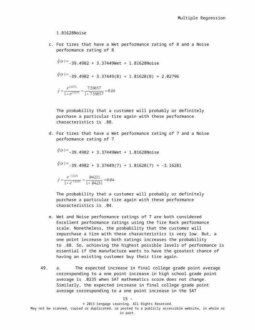
Thus, the estimated logit is -39.4982 + 3.37449Wet + 1.81628Noise
c. For tires that have a Wet performance rating of 8 and a Noise performance rating of 8
15 - © 2013 Cengage Learning. All Rights Reserved.
May not be scanned, copied or duplicated, or posted to a publicly accessible website, in whole or in part.

Multiple Regression
-39.4982 + 3.37449Wet + 1.81628Noise
-39.4982 + 3.37449(8) + 1.81628(8) = 2.02796
The probability that a customer will probably or definitely purchase a particular tire again with these performance characteristics is .88.
d. For tires that have a Wet performance rating of 7 and a Noise performance rating of 7
-39.4982 + 3.37449Wet + 1.81628Noise
-39.4982 + 3.37449(7) + 1.81628(7) = -3.16281
The probability that a customer will probably or definitely purchase a particular tire again with these performance characteristics is .04.
e. Wet and Noise performance ratings of 7 are both considered Excellent performance ratings using the Tire Rack performance scale. Nonetheless, the probability that the customer will repurchase a tire with these characteristics is very low. But, a one point increase in both ratings increases the probability to .88. So, achieving the highest possible levels of performance is essential if the manufacture wants to have the greatest chance of having an existing customer buy their tire again.
49. a. The expected increase in final college grade point average corresponding to a one point increase in high school grade point average is .0235 when SAT mathematics score does not change. Similarly, the expected increase in final college grade point average corresponding to a one point increase in the SAT mathematics score is .00486 when the high school grade point average does not change.
b. = -1.41 + .0235(84) + .00486(540) = 3.19
50. a. Job satisfaction can be expected to decrease by 8.69 units with a one unit increase in length of service if the wage rate does not change. A dollar increase in the wage rate is associated with a 13.5 point increase in the job satisfaction score when the length of service does not change.
b. = 14.4 - 8.69(4) + 13.5(6.5) = 67.39
51. a. The computer output with the missing values filled in is as follows:
The regression equation is
Y = 8.103 + 7.602 X1 + 3.111 X2
Predictor Coef SE Coef T Constant 8.103 2.667 3.04 X1 7.602 2.105 3.61
15 - © 2013 Cengage Learning. All Rights Reserved.
May not be scanned, copied or duplicated, or posted to a publicly accessible website, in whole or in part.
Chapter 15
X2 3.111 0.613 5.08
S = 3.35 R-sq = 92.3% R-sq (adj) = 91.0%
Analysis of Variance
SOURCE DF SS MS FRegression 2 1612 806 71.82Residual Error 12 134.67 11.2225Total 14 1746.67
b. F.05 = 3.89
F = 71.82 > F.05; significant relationship
Actual p-value = .000
Because p-value = .05, the overall relationship is significant
c. Using t table (12 degrees of freedom), area in tail corresponding to t = 3.61 is less than .005; p-value is less than .01
Actual p-value = .0000
Because p-value reject H0 : = 0
Using t table (12 degrees of freedom), area in tail corresponding to t = 5.08 is less than .005; p-value is less than .01
Actual p-value = .0003
Because p-value reject H0 : = 0
d. See computer output.
e.
52. a. The regression equation is
Y = -1.41 + .0235 X1 + .00486 X2
Predictor Coef SE Coef TConstant -1.4053 0.4848 -2.90X1 0.023467 0.008666 2.71X2 .00486 0.001077 4.51
S = 0.1298 R-sq = 93.7% R-sq (adj) = 91.9%
Analysis of Variance
SOURCE DF SS MS FRegression 2 1.76209 .881 52.44
15 - © 2013 Cengage Learning. All Rights Reserved.
May not be scanned, copied or duplicated, or posted to a publicly accessible website, in whole or in part.

Multiple Regression
Residual Error 7 .1179 .0168Total 9 1.88000
b. Using F table (2 degrees of freedom numerator and 7 degrees of freedom denominator), p-value is less than .01
Actual p-value = .0001
Because p-value there is a significant relationship.
c. for : p-value = .0302; reject H0: = 0
for : p-value = .0028; reject H0: = 0
d.
good fit
53. a. The regression equation is
Y = 14.4 - 8.69 X1 + 13.52 X2
Predictor Coef SE Coef TConstant 14.448 8.191 1.76X1 -8.69 1.555 -5.59X2 13.517 2.085 6.48
S = 3.773 R-sq = 90.1% R-sq (adj) = 86.1%
Analysis of Variance
SOURCE DF SS MS FRegression 2 648.83 324.415 22.79Residual Error 5 71.17 14.234Total 7 720.00
b. F.05 = 5.79
F = 22.79 > F.05; significant relationship.
Actual p-value = .0031
Because p-value ≤ α = .05, the overall relationship is significant.
c.
15 - © 2013 Cengage Learning. All Rights Reserved.
May not be scanned, copied or duplicated, or posted to a publicly accessible website, in whole or in part.

Chapter 15
good fit
d. for : t = p-value = .0025; reject H0 : = 0
for : p-value = .0013; reject H0 : = 0
54. a. A portion of the Minitab output follows:
The regression equation isBuy Again = - 7.52 + 1.82 Steering
Predictor Coef SE Coef T PConstant -7.522 1.467 -5.13 0.000Steering 1.8151 0.1958 9.27 0.000
S = 0.841071 R-Sq = 84.3% R-Sq(adj) = 83.3%
Analysis of Variance
Source DF SS MS F PRegression 1 60.787 60.787 85.93 0.000Residual Error 16 11.318 0.707Total 17 72.105
Because the p-value = .000 < α = .05, there is a significant relationship.
b. The estimated regression equation provided a good fit; 84.3 % of the variability in the Buy Again rating was explained by the linear effect of the Steering rating.
c. A portion of the Minitab output follows:
The regression equation isBuy Again = - 5.39 + 0.690 Steering + 0.911 Treadwear
Predictor Coef SE Coef T PConstant -5.388 1.110 -4.86 0.000Steering 0.6899 0.2875 2.40 0.030Treadwear 0.9113 0.2063 4.42 0.001
S = 0.572723 R-Sq = 93.2% R-Sq(adj) = 92.3%
Analysis of Variance
Source DF SS MS F PRegression 2 67.185 33.592 102.41 0.000Residual Error 15 4.920 0.328Total 17 72.105
d. For the Treadwear independent variable, the p-value = .001 < α = .05; thus, the addition of
15 - © 2013 Cengage Learning. All Rights Reserved.
May not be scanned, copied or duplicated, or posted to a publicly accessible website, in whole or in part.

Multiple Regression
Treadwear is significant.
55. a. A portion of the Regression tool output follows.
Regression StatisticsMultiple R 0.8013R Square 0.6421Adjusted R Square 0.6409Standard Error 3.4123
Observations 309
ANOVAdf SS MS F Significance F
Regression 1 6413.2883 6413.2883 550.8029 1.79552E-70Residual 307 3574.5628 11.6435
Total 308 9987.8511
Coefficients Standard Error t Stat P-value Lower 95%Upper 95%
Intercept 41.0534 0.5166 79.4748 8.1E-207 40.0370 42.0699
Displacement -3.7232 0.1586 -23.4692 1.8E-70 -4.0354 -3.4110
Because the p-value corresponding to F = 550.8029 is .0000 < = .05, there is a significant relationship.
b. A portion of the Excel Regression tool output follows.
Regression StatisticsMultiple R 0.8276R Square 0.6849Adjusted R Square 0.6829Standard Error 3.2068
Observations 309
ANOVA
15 - © 2013 Cengage Learning. All Rights Reserved.
May not be scanned, copied or duplicated, or posted to a publicly accessible website, in whole or in part.
Chapter 15
df SS MS F Significance FRegression 2 6841.0876 3420.5438 332.6232 1.79466E-77Residual 306 3146.7635 10.2835
Total 308 9987.8511
Coefficients Standard Error t Stat P-value Lower 95%Upper 95%
Intercept 40.5946 0.4906 82.7379 1.8E-211 39.6291 41.5600Displacement -3.1944 0.1701 -18.7745 7.43E-53 -3.5292 -2.8596
FuelPremium -2.7230 0.4222 -6.4498 4.37E-10 -3.5537 -1.8922
c. For FuelPremium, the p-value corresponding to t = -6.4498 is .000 < = .05; significant. The addition of the dummy variables is significant.
d. A portion of the Excel Regression tool output follows.
Regression StatisticsMultiple R 0.8554R Square 0.7317Adjusted R Square 0.7282Standard Error 2.9688
Observations 309
ANOVAdf SS MS F Significance F
Regression 4 7308.5436 1827.1359 207.3108 1.54798E-85Residual 304 2679.3075 8.8135
Total 308 9987.8511
Coefficients Standard Error t Stat P-value Lower 95%Upper 95%
Intercept 37.9626 0.7892 48.1055 3.5E-144 36.4097 39.5155Displacement -3.2418 0.1941 -16.7007 6.97E-45 -3.6238 -2.8599FuelPremium -2.1352 0.4519 -4.7253 3.52E-06 -3.0243 -1.2460FrontWheel 3.0747 0.5394 5.7005 2.83E-08 2.0133 4.1360
RearWheel 3.3114 0.5413 6.1174 2.92E-09 2.2462 4.3765
e. Since the p-value corresponding to F = 207.3108 is .0000 < = .05, there is a significant overall relationship. Because the p-values for each independent variable are also < = .05, each of the independent variables is significant.
15 - © 2013 Cengage Learning. All Rights Reserved.
May not be scanned, copied or duplicated, or posted to a publicly accessible website, in whole or in part.

Multiple Regression
56. a. Type of Fund is a categorical variable with three levels. Let FundDE = 1 for a domestic equity fund and FundIE = 1 for an international fund. The Excel output is shown below:
Regression StatisticsMultiple R 0.7838R Square 0.6144Adjusted R Square 0.5960Standard Error 5.5978
Observations 45
ANOVAdf SS MS F Significance F
Regression 2 2096.8489 1048.4245 33.4584 2.03818E-09Residual 42 1316.0771 31.3352
Total 44 3412.9260
Coefficients Standard Error t Stat P-value Lower 95% Upper 95%Intercept 4.9090 1.7702 2.7732 0.0082 1.3366 8.4814FundDE 10.4658 2.0722 5.0505 9.033E-06 6.2839 14.6477
FundIE 21.6823 2.6553 8.1658 3.288E-10 16.3237 27.0408
= 4.9090+ 10.4658 FundDE + 21.6823 FundIE
Since the p-value corresponding to F = 33.4584 is .0000 < = .05, there is a significant relationship.
b. R Square = .6144. A reasonably good fit using only Type of Fund.
c. The Excel output follows:
Regression StatisticsMultiple R 0.8135R Square 0.6617Adjusted R Square 0.6279Standard Error 5.3726Observations 45
ANOVA
15 - © 2013 Cengage Learning. All Rights Reserved.
May not be scanned, copied or duplicated, or posted to a publicly accessible website, in whole or in part.

Chapter 15
df SS MS F Significance FRegression 4 2258.3432 564.5858 19.5598 5.48647E-09Residual 40 1154.5827 28.8646Total 44 3412.9260
Coefficients Standard Error t Stat P-value Lower 95% Upper 95%Intercept 1.1899 2.3781 0.5004 0.6196 -3.6164 5.9961FundDE 6.8969 2.7651 2.4942 0.0169 1.3083 12.4854FundIE 17.6800 3.3161 5.3315 4.096E-06 10.9778 24.3821Net Asset Value ($) 0.0265 0.0670 0.3950 0.6950 -0.1089 0.1619Expense Ratio (%) 6.4564 2.7593 2.3399 0.0244 0.8798 12.0331
Since the p-value corresponding to F = 19.5558 is .0000 < = .05, there is a significant relationship.
For Net Asset Value ($), the p-value corresponding to t = .3950 is .6950 > = .05, Net Asset Value ($) is not significant and can be deleted from the model.
d. Morningstar Rank is a categorical variable. The data set only contains funds with four ranks (2-Star through –5Star), so three dummy variables are needed. Let 3StarRank = 1 for a 3-StarRank, 4StarRank = 1 for a 4-StarRank, and 5StarRank = 1 for a 5-StarRank. The Excel output follows:
Regression StatisticsMultiple R 0.8501R Square 0.7227Adjusted R Square 0.6789Standard Error 4.9904
Observations 45
ANOVAdf SS MS F Significance F
Regression 6 2466.5721 411.0954 16.5072 2.96759E-09Residual 38 946.3539 24.9040
Total 44 3412.9260
Coefficients Standard Error t Stat P-value Lower 95% Upper 95%Intercept -4.6074 3.2909 -1.4000 0.1696 -11.2694 2.0547FundDE 8.1713 2.2754 3.5912 0.0009 3.5650 12.7776FundIE 19.5194 2.7795 7.0227 2.292E-08 13.8926 25.1461Expense Ratio (%) 5.5197 2.5862 2.1343 0.0393 0.2843 10.75523StarRank 5.9237 2.8250 2.0969 0.0427 0.2048 11.64264StarRank 8.2367 2.8474 2.8927 0.0063 2.4725 14.0009
5StarRank 6.6241 3.1425 2.1079 0.0417 0.2624 12.9858
15 - © 2013 Cengage Learning. All Rights Reserved.
May not be scanned, copied or duplicated, or posted to a publicly accessible website, in whole or in part.
Multiple Regression
= -4.6074 + 8.1713 FundDE + 19.5194 FundIE +5.5197 Expense Ratio (%) + 5.9237 3StarRank + 8.2367 4StarRank + 6.6241 5StarRank
At the .05 level of significance, all the independent variables are significant.
e. = -4.6074 + 8.1713(1) + 19.5194(0) +5.5197(1.05) + 5.9237(1) + 8.2367(0) +6.62415(0) = 15.28%
57. a. A portion of the Minitab output is shown below:
The regression equation isSalaried ($1000s) = 40.3 + 1.19 Hourly ($1000s)
Predictor Coef SE Coef T PConstant 40.35 15.66 2.58 0.016Hourly ($1000s) 1.1947 0.3050 3.92 0.001
S = 30.2639 R-Sq = 35.4% R-Sq(adj) = 33.1%
Analysis of Variance
Source DF SS MS F PRegression 1 14049 14049 15.34 0.001Residual Error 28 25645 916Total 29 39694
b. Because the p-value = .001 < α = .05, there is a significant relationship.
c. A portion of the Minitab output is shown below:
The regression equation isSalaried ($1000s) = 27.0 + 1.22 Hourly ($1000s) - 3.2 Size-Midsize + 34.4 Size-Small
Predictor Coef SE Coef T PConstant 26.97 14.00 1.93 0.065Hourly ($1000s) 1.2240 0.2581 4.74 0.000Size-Midsize -3.21 12.63 -0.25 0.802Size-Small 34.40 10.44 3.30 0.003
S = 25.4752 R-Sq = 57.5% R-Sq(adj) = 52.6%
Analysis of Variance
Source DF SS MS F PRegression 3 22820.3 7606.8 11.72 0.000Residual Error 26 16873.6 649.0Total 29 39693.9
e. Hourly ($1000s): Significant because the p-value = .000 < α = .05.
Size-Midsize: Not significant because the p-value = .802 > α = .05
Size-Small: Significant because the p-value = .003 < α = .05
15 - © 2013 Cengage Learning. All Rights Reserved.
May not be scanned, copied or duplicated, or posted to a publicly accessible website, in whole or in part.

Chapter 15
f. A portion of the Minitab output using Hourly ($1000s) and Size-Small as the independent variables follows.
The regression equation isSalaried ($1000s) = 26.3 + 1.22 Hourly ($1000s) + 35.4 Size-Small
Predictor Coef SE Coef T PConstant 26.26 13.49 1.95 0.062Hourly ($1000s) 1.2176 0.2524 4.82 0.000Size-Small 35.409 9.486 3.73 0.001
S = 25.0299 R-Sq = 57.4% R-Sq(adj) = 54.2%
Analysis of Variance
Source DF SS MS F PRegression 2 22778 11389 18.18 0.000Residual Error 27 16915 626Total 29 39694
Source DF Seq SSHourly ($1000s) 1 14049Size-Small 1 8730
15 - © 2013 Cengage Learning. All Rights Reserved.
May not be scanned, copied or duplicated, or posted to a publicly accessible website, in whole or in part.