does regulatory capital arbitrage, reputation, or...
TRANSCRIPT

Does Regulatory Capital Arbitrage, Reputation,or Asymmetric Information Drive Securitization?
BRENT W. AMBROSE*
University of Kentucky
MICHAEL LACOUR-LITTLE**
California State University, Fullerton
ANTHONY B. SANDERS
The Ohio State University
Abstract
Banks can choose to keep loans on balance sheet as private debt or transform them into public debt via asset
securitization. Securitization transfers credit and interest rate risk, increases liquidity, augments fee income, and
improves capital ratios. Yet many lenders still retain a portion of their loans in portfolio. Do lenders exploit
asymmetric information to sell riskier loans into the public markets or retain riskier loans in portfolio? If riskier
loans are indeed retained in portfolio, is this motivated by regulatory capital incentives (regulatory capital
arbitrage), or a concern for reputation? We examine these questions empirically and find that securitized
mortgage loans have experienced lower ex-post defaults than those retained in portfolio, providing evidence
consistent with either the capital arbitrage or reputation explanation for securitization.
Key words: Banks, debt, securitization, regulatory capital.
Securitization is one of the major financial innovations to have occurred over recent
decades (Greenspan, 1998). In securitization, heterogeneous and illiquid individual loans
are combined into relatively homogeneous pools and transformed into highly liquid
bonds traded in dealer markets and generically referred to as asset-backed securities.
Such assets now permeate fixed income portfolios at both the institutional and individual
investor level. While the largest and most well known example of securitization is the
residential mortgage market, over the past decade securitization has spread rapidly into
home equity loan markets, commercial loan markets, credit card receivables, auto loans,
small-business loans, corporate loans, and other loan types. Although better developed in
the U.S. than in most other industrialized nations, securitization is expanding into foreign
markets as well [see, for example, Taylor (1996) for a summary of securitization activity
in European markets].
* Please address correspondence to Brent W. Ambrose, University of Kentucky, Gatton College of
Business and Economics, Lexington, KY 40506-0053. E-mail: [email protected].
** Research completed while affiliated with Washington University in St. Louis.
Journal of Financial Services Research, 28:1/2/3 113–133, 2005# 2005 Springer Science + Business Media, Inc. Manufactured in The Netherlands.

Asset securitization creates value by increasing liquidity, reducing or reallocating
credit or interest rate risk, improving leverage ratios, and allowing recognition of
accounting gains. Moreover, many of these securities provide the raw material for
synthetic securities traded in derivatives markets, expanding the market for the underlying
asset. In the process, financial re-engineering can create entirely new cash flow patterns
tailored to meet diverse clientele needs. Investors are attracted to the spread over
government security rates on asset-backed securities and trade off liquidity, interest rate,
call, and credit risk for the higher yields available in the asset-backed market.1
According to the Bond Market Association, as of the end of the first quarter of 2004,
the asset-backed market comprised just under one-third of the total $22.5 trillion bond
market. Within this category, mortgage-related assets were the largest component,
comprising approximately $5.3 trillion, with other asset-backed securities totaling $1.7
trillion. The combined category, and even the mortgage-related category alone, exceeds
the size of the Treasury market ($3.7 trillion) or the corporate bond market ($4.5 trillion).
Yet banks and thrifts still hold approximately $2.6 trillion in mortgage loans on their
balance sheets, representing about one-third of all outstanding mortgage debt (including
both public and private forms). How and why has this pattern developed?
Securitization first appeared in the residential mortgage market in the early 1980s and
received a major boost when the Tax Reform Act of 1986 incorporated legislation
authorizing real estate mortgage investment conduits (REMICs), a tax- and accounting-
favored structure under which assets to be securitized are transferred to a bankruptcy-
remote trust, thereby insulating the performance of securities issued from the financial
position of the issuer.2 As a result, by 1993, private issuers accounted for 15 percent of
total mortgage-backed securities volume (Korrell, 1996).
Furthermore, in the U.S. mortgage market, a well-developed institutional structure
exists to facilitate securitization for the majority of loans. Freddie Mac and Fannie Mae
(together the government-sponsored enterprises, the agencies, or the GSEs) were
chartered by Congress specifically to create a secondary market in mortgage debt to
ensure the continued availability of funds for housing finance.3 Both agencies purchase
1 See Bernardo and Cornell (1997) for an empirical analysis of Wall Street pricing of derivatives backed by
mortgage-backed securities.
3 Initially, Fannie Mae created a market for government-insured mortgage loans and Freddie Mac created an
analogous market for conventional loans, at that time originated mainly by savings institutions.
2 Ranieri (1996) traces the origins of securitization in the United States to the late 1970s when the word itself
first appeared in the Wall Street Journal. Kendall (1996) discusses the institutional requirements for
securitization to develop. Furthermore, Thomas (2001) notes that securitization is a natural response to
information asymmetries arising from project financing as well as comparative advantages in loan
servicing. For example, the signaling model developed by Greenbaum and Thakor (1987) suggests that
securitization allows financing of projects having significant information asymmetry between borrower and
lender, while the risk allocation models of Benveniste and Berger (1987) and James (1988) indicate that
securitization overcomes potential wealth transfers from shareholders to depositors, allowing lenders to
fund projects that otherwise would not be funded. As a result, securitization is a natural response to the
underinvestment problem proposed by Myers (1977), which suggests that firms may forgo profitable
investment opportunities if such investments result in possible wealth transfers from equity holders to debt
holders.
114 AMBROSE ET AL.

loans under either cash or swap programs (Fabozzi and Dunlevy, 2001). In the swap
program, large pools of loans are swapped with a single lender in return for a mortgage-
backed security collateralized by the same pool of loans. Interest on the pool of loans
covers servicing costs, typically paid to the originator, a guarantee fee paid to the agency,
and the balance of the available interest payments are available for the coupon on the
security. Under the cash program, the agencies purchase smaller pools of loans and
combine them into larger multi-lender pools and issue securities backed by them. In
either case, the originator can realize all loan fees collected in excess of costs as current
period profits and can continue to earn ongoing fees for loan servicing with limited
balance-sheet exposure and without any credit risk.4
After authorization of REMICs in 1986, a market in non-agency mortgage-backed
securities also developed. Non-conforming loans may be securitized in these private-
label issues, though alternative credit enhancement structures are required, since
guarantees are not available from the agencies. Non-conforming loans are either too
large to meet conforming size limits ( jumbos) or do not meet agency underwriting
guidelines (Alt-A or subprime). Typically, multi-class securities are issued with sub-
ordinate tranches bearing most of the credit risk. In this case, credit risk may not be
completely transferred, since issuers sometimes retain subordinate pieces of the security.
Collateralized mortgage obligations (CMOs) further reallocate risk by prioritizing receipt
of amortization, both scheduled and unscheduled prepayments, to allow expected matu-
rities to be more precisely defined.5
Regardless of the mode or outlet, securitization increases liquidity for the originator.
Under the agency swap program, the originator receives a liquid asset in the form of a
mortgage-backed security; under the cash program, the lender has cash proceeds to
reinvest, either in additional mortgage lending or in alternative liquid instruments, such
as Treasury securities. Under a non-agency REMIC structure, the lender will receive cash
proceeds net of transaction costs from sale of the multi-class securities issued.
For banks, an additional benefit is that securitization reduces the level of regulatory
capital required. Under current Basel capital rules, residential mortgage loans that have
been prudently underwritten generally require a 50 percent risk weighting, i.e., 2 percent
capital (50 percent times the 4 percent standard Tier 1 capital requirement), whereas
agency securities require only a 20 percent risk weighting, i.e., 0.8 percent capital. For
details on the bank capital rules and current proposals to make requirements better
conform to actual risk levels, see Calem and LaCour-Little (2004). They argue that, for
most mortgage loans, existing regulatory capital levels are too high, creating an incentive to
securitize the least risky loans. Furthermore, Passmore et al. (2002) demonstrate that the
incentive to securitize loans declines as regulatory capital requirements increase. Con-
4 This assumes the originator’s credit quality is sufficient to sell loans on a non-recourse basis, which is not
always the case. If lenders produce poor quality loans, the GSEs may condition future purchases on
recourse.
5 The CMO structure channels mortgage principal payments (both amortization and prepayments) to a series
of bonds. As of year-end 2002, almost $1.0 trillion in agency CMOs were outstanding. (Source: The Bond
Market Association).
SECURITIZATION 115

sistent with some of the literature, we refer to the decision to hold an asset in securitized
form to minimize regulatory capital requirements as regulatory capital arbitrage.
In addition to regulatory capital rules favoring securitization, the presence of
information asymmetries may also encourage securitization. If we assume that the
lender is better informed about the borrower’s credit quality than are the purchasers of
the securitized debt, then the purchasers of securitized debt may set credit standards that
are higher than those of the lender in order to protect themselves against the possible
Blemons market^ outcome suggested by Akerlof (1970). For example, DeMarzo and
Duffie (1999) using a liquidity-based model of securitization show that if asymmetric
information results in the lender’s facing a downward sloping demand curve for its
mortgage-backed security, then an optimal strategy is to retain a portion of the loans
in portfolio. Their model implies that if the issuer does not wish to retain any portion
of the mortgage-backed security, then she should sell only those loans having the lowest
degree of asymmetric information into the pool and retain those loans with a high degree
of asymmetric information. Hence, the lender may retain loans that are higher risk
(and have higher rate spreads) than those sold to the secondary loan market.6 As a result,
we would predict that retained loans have a higher incidence of default than those sold to
the secondary market. Alternatively, DeMarzo (2005) develops a model in which
informed financial intermediaries with superior information about asset valuation buy
pools of loans and enhance their returns on capital by creating derivative securities by
Btranching^ those pools based on specific risk characteristics. Since such activities are
undertaken mainly by secondary market participants, including major investment banks, the
issue is not directly relevant to the primary market participant issue of whether to retain or
securitize.
If lenders wish to reduce regulatory capital requirements, transfer credit and interest
rate risk, and increase liquidity, then we would expect to see most loans securitized. On
the other hand, if firms prefer diversification to specialization, they may retain some
percentage of the loans in their portfolio (see Winton (2000) for a discussion of diver-
sification versus specialization in lending). If existing risk-based capital rules require too
much capital for low-risk loans and too little capital for high-risk loans, we would expect
to see the low-risk loans securitized and the high-risk loans retained in portfolio.
Furthermore, since banks typically have ongoing contracts to sell loans to one of the
two major government sponsored enterprises operating in the secondary market, they
have an interest in maintaining their reputation for credit quality so as not to lose market
access. This repeated game structure with a relatively limited set of loan buyers
reinforces our expectation that securitized loans should be relatively safer than those
retained in portfolio. Unfortunately, we are unable to separate the reputation hypothesis
from the regulatory capital arbitrage hypothesis in our empirical tests: both hypotheses
predict that securitized loans should have lower default rates than loans retained in
portfolio.
6 Although the presence of asymmetric information and risk are correlated, they are not the same.
116 AMBROSE ET AL.

In this paper, we empirically examine the ex-post performance of securitized and
unsecuritized loans with the goal of determining whether securitization is a natural by-
product of information asymmetries present in the loan market or whether securitization
occurs in response to lender incentives resulting from bank capital regulations or a
concern for reputation. Our analysis is based on approximately 14,000 mortgage loans
originated between 1995 and 1997 and observed through October 2000. These loans
represent a broad spectrum of the mortgage market (both conventional and jumbo) with
approximately 95 percent being ultimately securitized. Our empirical analysis follows a
two-step process. First, we estimate a competing risks hazard model of mortgage
termination based on the prepayment and default status of the mortgages originated in
1995 and 1996 using only data available at the time of mortgage origination. The purpose
of this first step is to estimate a model that will provide a prediction of the prepayment
and default probability for mortgages originated in 1997. The second step of our analysis
uses these predicted probabilities as explanatory factors in assessing the probability that a
mortgage originated in 1997 is either securitized or held in portfolio. This mortgage
securitization model also includes a measure of whether the loans have relatively high or
low origination effective yield spreads, thus providing a means for testing whether
lenders use asymmetric information in making securitization decisions.
To preview the empirical findings, we find that higher risk loans are indeed retained in
portfolio, while lower risk loans are securitized, confirming the implications of Calem
and LaCour-Little (2004) and DeMarzo and Duffie (1999). Although the results from our
study appear to support the regulatory capital arbitrage or the repeated games reputation
hypotheses, it is important to remember that these data represent a relatively small
portion of the overall volume of mortgage origination activity by a single lender and,
thus, may not generally apply to the broader market.
1. Data
The data used for this research consist of event histories on 14,285 conventional fixed
rate mortgages originated between January 1995 and December 1997 and followed
through October 2000. Both conforming and non-conforming loans are included,
Table 1. Distribution of mortgage loans by origination year
This table reports the frequency distribution by year for the sample of 14,285 conventional fixed rate mortgage
loans originated between January 1995 and December 1997 by a national lender that prefers anonymity. Both
conforming and non-conforming loans are included, although super-jumbos (loans with initial balances in
excess of $650,000) are not. Loans were originated throughout the United States and were tracked from
origination through October 2000.
Year Frequency Percent
Mortgage outcome
Prepaid Default Still active
1995 4,695 32.9 2,048 340 2,307
1996 3,265 22.9 1,421 167 1,677
1997 6,325 44.3 1,700 380 4,245
Total 14,285 100.0 5,169 887 8,229
SECURITIZATION 117

although super-jumbos (loans with initial balances in excess of $650,000) are not. Loans
were originated throughout the United States. Table 1 reports the distribution of the loans
by origination year and outcome.
Table 2 shows the geographic distribution of the sample. Since our data come from a
single lender, we compared the sample distribution to the MIRS and Home Mortgage
Disclosure Act (HMDA) databases. The distribution of mortgage originations across
years follows a pattern similar to that observed in the broader market. However, the
comparison indicates that our sample is somewhat overrepresented by loans in the
New York/New Jersey region and underrepresented in the Northwest and Southwest
regions.7
We have relatively complete micro-level data for each loan in the sample, including
geographic location, loan amount, note rate, and points paid at time of loan origination.8
We also observe major credit quality indicators, including loan-to-value ratio (LTV ) and
borrower credit score at time of origination (FICO).9 Borrower characteristics available
include age (BRWAGE) and income (INCOME). Table 3 reports the descriptive statistics
for the sample, segmented by origination year and outcome. In general, we find that loans
sold to the GSEs had lower loan-to-value ratios at origination than loans held in portfolio
or sold as private-label MBS. Across origination years, we see a general decline in LTV
in the later years, which is consistent with greater refinancing activity in 1996 and 1997 than
in 1995.
Table 2. Distribution of mortgages across origination year, geographic region and by outcome (percent
of total loans originated in each year by region and outcome)
HUD region
Held in portfolio Sold to GSE Sold to private label
1995 1996 1997 1995 1996 1997 1995 1996 1997
1: New England 2.8% 1.2% 1.6% 3.5% 3.4% 4.2% 1.8% 4.8% 6.8%
2: New York/New Jersey 35.0% 65.2% 65.8% 34.0% 37.5% 35.7% 24.0% 29.2% 28.7%
3: Mid-Atlantic 6.5% 9.9% 11.9% 7.2% 7.4% 9.9% 11.4% 14.7% 12.5%
4: Southeast 3.5% 4.3% 6.2% 10.9% 11.9% 11.3% 6.0% 6.0% 5.7%
5: Midwest 17.6% 6.8% 2.6% 19.0% 19.8% 16.7% 12.1% 13.9% 12.7%
6: Southwest 0.0% 0.6% 0.0% 6.4% 3.5% 4.0% 0.9% 1.5% 1.3%
7: Great Plains 7.8% 1.2% 0.5% 6.4% 3.5% 2.6% 2.0% 0.2% 1.0%
8: Rocky Mountain 0.0% 0.6% 1.0% 1.9% 1.2% 1.4% 0.1% 1.1% 1.1%
9: Pacific 26.7% 9.9% 10.4% 9.7% 11.2% 13.3% 41.7% 28.3% 29.9%
10: Northwest 0.0% 0.0% 0.0% 0.9% 0.6% 0.9% 0.0% 0.3% 0.4%
Total Loans 397 161 193 2930 2485 4831 1368 619 1301
7 The Appendix provides a table detailing the comparison of our sample with the broader market.
8 Points paid at origination refers to the practice of charging borrowers interest at the time of mortgage
origination where one point equals 1 percent of the loan amount. The combination of points paid at
origination and the mortgage contract rate determine the effective yield (or cost) of the mortgage at
origination.
9 Borrower credit quality is measured by the credit score obtained from Fair, Isaac and Company (FICO).
Higher scores indicate high-quality borrowers and lower scores indicate lower quality.
118 AMBROSE ET AL.

Ta
ble
3.
Des
crip
tiv
est
ati
stic
s(s
tan
da
rdd
evia
tio
ns
rep
ort
edin
pa
ren
thes
es)
Th
ista
ble
rep
ort
sth
ed
escr
ipti
ve
stat
isti
csfo
rth
esa
mp
leo
f1
4,2
85
con
ven
tio
nal
fix
edra
tem
ort
gag
elo
ans
ori
gin
ated
bet
wee
nJa
nu
ary
19
95
and
Dec
emb
er1
99
7b
ya
nat
ion
alle
nd
erth
atp
refe
rsan
on
ym
ity
.B
oth
con
form
ing
and
no
n-c
on
form
ing
loan
sar
ein
clu
ded
,al
tho
ug
hsu
per
-ju
mb
os
(lo
ans
wit
hin
itia
lb
alan
ces
inex
cess
of
$6
50
,00
0)
are
no
t.
Var
iab
leL
abel
Hel
din
po
rtfo
lio
So
ldto
GS
Es
So
ldas
pri
vat
ela
bel
19
95
19
96
19
97
19
95
19
96
19
97
19
95
19
96
19
97
Nu
mb
ero
flo
ans
39
71
61
19
32
93
02
48
54
83
11
36
86
19
13
01
LT
VA
ver
age
LT
V0
.89
2
(0.1
3)
0.8
27
(0.1
7)
0.7
96
(0.1
7)
0.7
27
(0.1
8)
0.7
12
(0.1
7)
0.7
14
(0.1
7)
0.9
00
(0.1
1)
0.8
07
(0.1
5)
0.7
86
(0.1
5)
YL
DS
PD
Eff
ecti
ve
yie
ldV
10
-yr
Tre
asu
ryR
ate
2.0
39
(0.5
2)
1.7
18
(0.4
3)
1.7
90
(0.5
7)
1.8
43
(0.3
7)
1.6
34
(0.3
4)
1.5
33
(0.2
6)
1.8
39
(0.4
0)
1.6
49
(0.3
7)
1.5
66
(0.2
7)
FIC
OF
air
Isaa
c
Cre
dit
Sco
re
69
0.8
06
(63
.15
)
70
8.9
88
(61
.31
)
69
2.9
90
(67
.59
)
71
9.1
34
(58
.19
)
71
6.8
44
(58
.35
)
71
8.6
92
(60
.07
)
69
3.5
44
(60
.53
)
71
4.5
09
(58
.66
)
71
1.8
53
(58
.90
)
BR
WA
GE
Bo
rro
wer
Ag
e3
5.7
00
(9.6
8)
40
.50
3
(11
.50
)
42
.57
0
(12
.69
)
42
.63
0
(12
.12
)
44
.54
0
(12
.28
)
43
.84
7
(12
.05
)
36
.55
3
(9.4
8)
39
.94
0
(9.9
3)
40
.46
5
(9.6
7)
INC
OM
EB
orr
ow
erIn
com
e
(’0
00
s)
$5
1.9
76
($5
3.7
5)
$7
2.1
77
($1
80
.12
)
$7
2.0
48
($4
9.1
2)
$5
7.7
25
($4
5.7
2)
$5
9.8
23
($5
5.5
0)
$6
7.8
76
($5
3.9
2)
$5
7.2
20
($5
6.3
6)
$1
11
.88
4
($1
74
.39
)
$1
24
.36
2
($1
14
.62
)
OR
IBA
LL
oan
Am
ou
nt
$9
6,1
70
($6
3,5
86
)
$1
06
,52
4
($6
7,3
39
)
$1
23
,59
5
($8
3,9
72
)
$1
08
,08
1
($4
6,2
65
)
$1
09
,15
6
($4
6,9
46
)
$1
21
,79
6
($4
9,6
29
)
$1
32
,68
4
($9
7,3
20
)
$2
17
,94
3
($1
30
,94
6)
$2
64
,89
3
($1
32
,94
8)
Nu
mb
ero
fP
rep
ays
23
56
55
71
,33
61
,07
91
,18
04
77
27
74
63
Nu
mb
ero
fD
efau
lts
64
16
23
13
61
15
26
61
40
36
91
Nu
mb
erS
till
Cu
rren
t9
88
01
13
1,4
58
1,2
91
3,3
85
75
13
06
74
7
SECURITIZATION 119

In general, credit quality appears to have increased year over year, with declining
LTVs and increasing credit scores. However, we note that differences do exist across
the three samples. In general, borrower credit quality is lower for loans held in portfolio
and highest for loans sold to the GSEs. For example, in 1997 borrower credit scores
averaged 693 for loans held in portfolio versus 719 for loans sold to the GSEs. We also
find smaller differences in borrower age at origination (our proxy for wealth), with
loans sold to the GSEs having a higher average borrower age. However, loans sold to
the GSEs have lower average borrower income at origination. Consistent with housing
market appreciation, loan amounts increased over time, and we find that loan amounts
for loans sold as private-label MBS are consistently greater than loans held in portfolio
or sold to the GSEs. For example, loans sold as private label had an average balance
in 1997 of $264,900, while the average loan balance for loans held in portfolio was
$123,600.
Overall, we note that 72 percent (10,246) of the loans were sold to the GSEs, 23
percent (3,288) were sold as private-label MBS, and 5 percent (751) were retained in the
lender’s portfolio. However, the breakdown by origination year indicates a subtle trend
away from retaining loans in portfolio. For example, in 1995 we see that 8.5 percent of
loans originated were retained in portfolio, but by 1997, only 3.1 percent of the loans
originated that year were retained. As a result, we see a corresponding increase in the
percentage of loans that were sold into the secondary market.
We can identify at least two possible reasons for this shift in loan disposition. First, it
could simply result from changes in average borrower characteristics over time, with
more borrowers meeting secondary market standards seeking loans in 1997 than in 1995.
This would be consistent with the observed increase in mortgage refinancing that
occurred during 1997 as interest rates fell. On the other hand, the observed change in
loan disposition may represent a shift in risk preferences by the lender.
Table 3 also reports the average mortgage yield spread at origination (YLDSPD),
calculated as the effective mortgage yield, including the effect of any points paid at
origination and assuming a 10-year holding period, less the 10-year constant maturity
Treasury rate. We note that loans held in portfolio have higher origination spreads and
that the spreads on loans sold into the secondary market (either as private label or to the
GSEs) are roughly the same. However, we do note a general decline in the origination
spread over the three-year period.
2. Ex-post defaults and prepayments on securitized and portfolio loans
In this section, we estimate an empirical model of prepayment and default using
borrower information available to the lender at the time of underwriting. The purpose of
this model is to estimate a priori prepayment and default probabilities for each borrower.
We use these estimated probabilities in the next section to examine the risk profile of
loans that are securitized versus those that are retained in portfolio.
It is well known that a mortgage borrower has the option to prepay the mortgage,
default, or continue the mortgage by making the payment due. In estimating a competing
120 AMBROSE ET AL.

risks model, we denote mortgages that are still current at the end of the observation
period as censored. Thus, we define Tj ( j = 1, 2, 3) as the latent duration for each loan to
end during the observation window by prepaying, defaulting, or being censored and the
observed duration, � , is the minimum of the Tj.
Conditional on a set of explanatory variables, xj, that include personal characteristics
as well as market conditions at the time of origination, and parameters, �j, the probability
density function ( pdf ) and cumulative density function (cdf ) for Tj are
fj Tj xj; �j
��
� �
¼ hj Tj xj; �j
��
� �
exp �Ij rj xj; �j
��
� �� �
; ð1Þ
Fj Tj xj; �j
��
� �
¼ 1� exp �Ij rj xj; �j
��
� �� �
; ð2Þ
where r is an integer variable taking values in the set {1,2,3} representing the three
possible outcomes, Ij is the integrated hazard for outcome j:
Ij Tj xj; ���
� �
¼Z Tj
0
hj s xj; �j
��
� �
ds, ð3Þ
and hj is the hazard function.
The joint distribution of the duration and outcome is
f �; j x; �jð Þ ¼ hj � xj; �j
��
� �
exp �I0 � x; �jð Þð Þ, ð4Þ
where x = (x1, x2, x3), � = (�1, �2, �3) and I0 =P
Ij is the aggregated integrated hazard.
Thus, the conditional probability of an outcome is
Pr j �; x; �jð Þ ¼hj � xj; �
��
� �
P3
j¼1
hj � x; �jð Þ: ð5Þ
To simplify estimation, we specify a separate exponential hazard function for each
mortgage outcome
hj �j xj; �j
��
� �
¼ exp x 0j�j
� �
, ð6Þ
and estimate (5) in a multinomial logit framework.
Since the purpose of the competing risks model is to obtain an unbiased expectation of
borrower prepayment and default risk, we divide our sample into an estimation sample
and a holdout sample. We estimate (5) using the estimation sample. Using the estimated
coefficients, we then calculate the predicted prepayment and default probabilities for the
loans in the holdout sample. This scheme avoids introducing bias into the subsequent
analysis by using ex-ante outcome probabilities based on ex-post realizations. To only
SECURITIZATION 121

use information (or statistical inferences) available at loan origination, we place all loans
originated in 1995 or 1996 in the estimation sample and reserve the loans originated in
1997 as the holdout sample. Thus, we are using information about loans originated in
1995 and 1996, and followed for up to six years after origination, to develop empirical
prepayment and default models that will be used to calculate predicted prepayment and
default probabilities for loans originated in 1997.
Table 4 presents the parameter estimates of the competing risks model estimated from
the estimation sub-sample. Again, our purpose here is to obtain forward-looking pre-
payment and default probabilities, and thus, we only use information about the borrower
that was available at origination. Therefore, the set of explanatory variables (xj) includes
the borrower’s credit score (FICO) at origination, the borrower’s age and income at
origination (BRWAGE and INCOME ), the mortgage loan-to-value ratio at origination
(LTV ), the discount points paid by the borrower at origination (DISCPTS ), and a dummy
variable indicating whether the loan was eligible for sale to the GSEs at origination
Table 4. Competing risks model of mortgage outcome
Pr j �; x; �jð Þ ¼ hj � xj ;�jð ÞP3
j¼1
hj � x;�jð Þ
The competing risks model is estimated as a multinomial logit model assuming a quadratic baseline hazard
function. The odds ratio estimates are calculated as e� and provide an indication of the sensitivity of the
estimated probabilities to a change in that variable.
Variable Label
Coefficients Odds ratio estimates
Prepay Default Prepay Default
Intercept j8.521*** (814.93) j7.011*** (84.39)
FICO Fair Isaac Credit Score 0.002*** (26.90) j0.008*** (117.11) 1.00 0.99
BRWAGE Borrower Age j0.014*** (63.07) 0.002 (0.24) 0.99 1.00
INCOME Borrower Income 0.001*** (35.36) j0.002** (3.89) 1.00 1.00
LTV Loan-to-value Ratio j0.631*** (29.93) 1.178*** (10.25) 0.53 3.25
DISCPT Discount Points Paid at
Origination
j0.184*** (70.38) 0.014 (0.08) 0.83 1.01
q2 Non-judicial, No
Deficiency
0.212*** (20.14) 0.130 (1.29) 1.24 1.14
q3 Judicial & Deficiency 0.182*** (20.75) 0.011 (0.01) 1.20 1.01
q4 Judicial, No Deficiency 0.538*** (5.59) j9.291 (0.01) 1.71 <0.001
Conform 1 = conforming loan j0.037 (0.68) j0.264*** (5.92) 0.96 0.77
Time Number of months
since origination
0.232*** (1150.42) 0.271*** (178.28) 1.26 1.31
Time2 Time*Time j0.003*** (981.62) j0.003*** (146.18) 1.00 1.00
Likelihood Ratio
Statistic
2964.5***
(Chi-square statistics reported in parentheses)
***- Significant at the 1% level.
** -Significant at the 5% level.
* -Significant at the 10% level.
122 AMBROSE ET AL.

(CONFORM).10 Following Ambrose and Pennington-Cross (2000), who determine that
state mortgage laws are an important factor in determining the spatial distribution of
mortgage loans, we also include a set of dummy variables that classify states based on
judicial versus non-judicial foreclosure laws and deficiency versus non-deficiency
judgment states in order to control for differences in state laws regarding mortgage
default and foreclosure.11 q1 indicates states that have non-judicial foreclosure available
and allow lenders to obtain deficiency judgments;12 q2 indicates states that have non-
judicial foreclosure available but do not allow deficiency judgments;13 q3 indicates states
that require judicial foreclosure and allow deficiency judgments;14 and finally q4
indicates states that require judicial foreclosure and do not allow deficiency judgments.
Consistent with theoretical predictions, we note that the probability of prepayment
increases and the probability of default decreases with borrower credit quality. That is,
borrowers with higher FICO scores at origination are more likely to prepay and less
likely to default. The odds-ratio estimates indicate that every one point increase in
borrower credit quality at origination reduces the probability of default by 0.1 percent
and increases the probability of prepayment by a similar percentage. Furthermore, we
note that younger borrowers with higher incomes at origination have higher prepayment
probabilities. We see that the loan-to-value ratio at origination also has the expected
effect on prepayment and default, with the probability of prepayment declining and the
probability of default rising as the loan-to-value ratio at origination increases.
Furthermore, we see that discount points paid at origination have the expected impact
on prepayment. That is, borrowers who pay points are less likely to prepay.15 Not
surprisingly, given the underwriting guidelines established by Fannie Mae and
Freddie Mac, the competing risk estimation shows that mortgages that fall into the
Bconforming loan^ category have lower probabilities of prepayment and default.
Using the parameter estimates from table 4, we compute the predicted prepayment and
default probabilities for the borrowers in the holdout sub-sample. Table 5 reports the mean
predicted cumulative prepayment and default probabilities for 12, 24, 36, 48, and 60 months
after origination. Based on our estimated model, we find that the average probability of
prepayment for the first 12 months is 1.3 percent and the average probability of default is 0.1
10 Although we know the actual loan status at the time the dataset was created (i.e., whether sold to Fannie
Mae or Freddie Mac, sold to a private-label MBS, or retained in portfolio), we cannot precisely determine
whether the mortgage was conforming at origination. Thus, we classify a mortgage as conforming if it was
sold to the agencies, or if the borrower’s FICO score is above 660 and the loan amount was below the
conforming loan limit in place at time of origination and the LTV is either less than 80 percent or the loan
has private mortgage insurance if the LTV is greater than 80 percent.
11 Ambrose et al. (1997) provide theoretical justification for the impact of state borrower protection laws on
borrower prepayment and default propensity.
12 q1 indicates AL, AR, DC, GA, HI, MO, IA, MA, MD, MI, MS, RI, NE, NH, NM, NV, NY, TN, UT, VA,
WV, WY, CO.
13 q2 indicates AK, AZ, CA, ID, OK, ME, MN, MT, NC, OR, SD, TX, WA.
14 q3 indicates CT, DE, FL, IL, IN, KS, KY, NJ, OH, PA, SC, VT.
15 See Stanton and Wallace (1998) and Kau and Keenan (1987) for a discussion of the impact of mortgage
points on borrower prepayment.
SECURITIZATION 123

percent. As the mortgages season, the cumulative probability of prepayment rises to 44.4
percent by month 60 and the cumulative probability of default rises to 5.5 percent. These are
slightly higher default probabilities but lower prepayment probabilities, compared to
national averages for comparable vintages as reported by LoanPerformance.16
Table 5 also reports the predicted cumulative outcome probabilities based on the
disposition of the loan after origination. In general, we find that the prepayment proba-
bilities for mortgages retained in portfolio, sold to the GSEs, or sold as private-label
MBS are roughly the same. The prepayment probabilities for mortgages sold as private-
label MBS are slightly higher (46.2 percent by month 60 versus 44.1 percent for
mortgages sold to the GSEs or 39.2 percent for mortgages retained in portfolio).
However, we find that the probability of default is higher for mortgages retained in
portfolio than for loans sold to the secondary market. The cumulative probability of
default by month 60 is 8.7 percent for loans held in portfolio versus 5.1 percent for loans
sold to the GSEs and 6.7 percent for loans sold as private-label MBS. Again, this is
consistent with the observed pattern of the GSEs’ imposing tighter underwriting
standards on mortgages they will accept. In addition, the observed pattern is consistent
with our expectations concerning the loans that the lender would sell to the GSEs, given
the GSEs’ practice of requiring lenders to buy back defaulted mortgages if the default
experience is outside acceptable limits.
Table 5. Predicted cumulative prepayment and default probabilities
Predicted prepayment and default probabilities are calculated for each borrower in the holdout sample using the
estimated coefficients reported in table 4. Sample means reflect the expected cumulative prepayment and
default probabilities at 12, 24 36, 48, and 60 months since mortgage origination.
Full sample
N = 6,325
Held in portfolio
N = 193
Sold to GSEs
N = 4,831
Sold as
private label
N = 1,301
Mean Std. dev. Mean Std. dev. Mean Std. dev. Mean Std. dev.
Panel A: Cumulative Prepayment Probabilities
Month 12 0.013 0.003 0.011 0.003 0.013 0.003 0.014 0.004
Month 24 0.090 0.023 0.075 0.021 0.085 0.020 0.092 0.025
Month 36 0.245 0.056 0.215 0.067 0.242 0.053 0.259 0.064
Month 48 0.386 0.079 0.341 0.118 0.383 0.075 0.404 0.090
Month 60 0.444 0.087 0.392 0.144 0.441 0.083 0.462 0.099
Panel B: Cumulative Default Probabilities
Month 12 0.001 0.000 0.001 0.001 0.001 0.000 0.001 0.001
Month 24 0.006 0.004 0.009 0.006 0.005 0.003 0.007 0.005
Month 36 0.022 0.016 0.035 0.025 0.020 0.013 0.027 0.021
Month 48 0.043 0.031 0.068 0.048 0.040 0.026 0.053 0.041
Month 60 0.055 0.040 0.087 0.060 0.051 0.034 0.067 0.051
16 LoanPerformance reports current default rates for broad classes of loan categories and vintages, but not
cumulative rates. As of 2001, the current 90-day delinquency rate for conventional loans originated in
1995 was 1.53 percent and 1.47 percent for loans originated in 1996.
124 AMBROSE ET AL.

3. The decision to securitize
We now turn to the question of whether the predicted prepayment and default probabilities
have a systematic impact on the lender’s decision to securitize the loan. In the introduction,
we noted two possible theories for securitization. First, originators may wish to retain high-
default-risk loans and securitize low-default-risk loans in response to bank capital
regulations or reputation effects. Second, originators may take advantage of asymmetric
information to securitize less profitable loans (based on default and prepayment risk).17
With respect to the first theory, if bank capital regulations or lender reputation affect loan
portfolio decisions, then we would expect to find a positive relationship between expected
default probabilities and the probability of retaining the loan in portfolio. That is, high-
default-risk loans as revealed by higher expected default probabilities are more likely to
be retained in portfolio. The second theory suggests that originators will use inside
information to selectively securitize loans; that is, originators will securitize loans with
lower expected profitability. Here, the tradeoff between high risk (either prepayment or
default risk) and securitization is not as clear. The originator may find it more profitable
to keep higher-risk loans if the corresponding yield spread justifies the risk. This suggests
that we must examine the probability that a loan is retained in portfolio relative to
expected prepayment and default potential as well as loan yield spread at origination.
To determine whether a particular loan is over- or underpriced relative to other loans
originated by the lender, we follow Ambrose et al. (2004) and estimate an ordinary least
squares regression of the mortgage yield spread at origination. To control for char-
acteristics that affect mortgage yields, we follow the standard yield spread models
developed in the literature. We include independent variables loan amount; the mortgage
loan-to-value ratio; a dummy variable denoting whether the loan amount is above the
conforming loan limit; a dummy variable denoting whether the loan meets the GSE
conforming loan standards; the borrower’s credit quality score; a set of dummy variables
controlling for location; the current local house price and market interest rate volatilities;
the market credit risk premiumVdefined as the difference between the BAAA^ bond index
and the BBaa^ bond index; the yield curve slopeVcalculated as the difference between the
10-year and one-year Treasury bond rates; and a set of dummy variables that categorize
states based on judicial versus non-judicial foreclosure laws and deficiency versus non-
deficiency judgment states in order to control for differences in legal environment.18
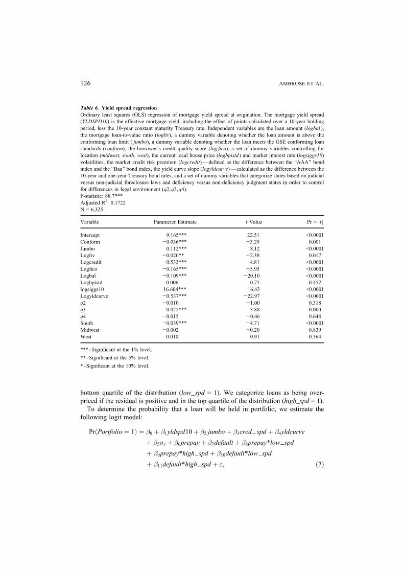
Table 6 reports the results of the OLS regression estimation for the loans originated
in 1997 (the holdout sample). All coefficient estimates have the expected signs. From this
estimation, we collect the residuals to provide an indication of which loans are over- or
underpriced relative to the other loans originated in 1997. Based on the distribution of the
residuals, we categorize loans as being underpriced if the residual is negative and in the
17 Asymmetric information between the lender and MBS investors regarding individual borrower loans could
result from a variety of sources. For example, the lender could gather additional information about the
borrower that is not usually contained in the standard underwriting documents through the interview
process with the loan officer or if the borrower has a prior relationship with the lending institution.
18 McKenzie (2002) provides an extensive survey of efforts to model empirical mortgage yield spreads.
SECURITIZATION 125
bottom quartile of the distribution (low_spd = 1). We categorize loans as being over-
priced if the residual is positive and in the top quartile of the distribution (high_spd = 1).
To determine the probability that a loan will be held in portfolio, we estimate the
following logit model:
Pr Portfolio ¼ 1ð Þ ¼ �0 þ �1yldspd10þ �2 jumboþ �3cred spd þ �4yldcurve
þ �5�r þ �6prepayþ �7default þ �8prepay*low spd
þ �9prepay*high spd þ �10default*low spd
þ �11default*high spd þ ", ð7Þ
Table 6. Yield spread regression
Ordinary least squares (OLS) regression of mortgage yield spread at origination. The mortgage yield spread
(YLDSPD10) is the effective mortgage yield, including the effect of points calculated over a 10-year holding
period, less the 10-year constant maturity Treasury rate. Independent variables are the loan amount (logbal ),
the mortgage loan-to-value ratio (logltv), a dummy variable denoting whether the loan amount is above the
conforming loan limit ( jumbo), a dummy variable denoting whether the loan meets the GSE conforming loan
standards (conform), the borrower’s credit quality score (log fico), a set of dummy variables controlling for
location (midwest, south, west), the current local house price (loghpistd ) and market interest rate (logsiggs10)
volatilities, the market credit risk premium (logcredit)Vdefined as the difference between the BAAA^ bond
index and the BBaa^ bond index, the yield curve slope (logyldcurve)Vcalculated as the difference between the
10-year and one-year Treasury bond rates, and a set of dummy variables that categorize states based on judicial
versus non-judicial foreclosure laws and deficiency versus non-deficiency judgment states in order to control
for differences in legal environment (q2,q3,q4).
F-statistic: 88.7***
Adjusted R2: 0.1722
N = 6,325
Variable Parameter Estimate t Value Pr > |t |
Intercept 9.165*** 22.51 <0.0001
Conform j0.036*** j3.29 0.001
Jumbo 0.112*** 8.12 <0.0001
Logltv j0.020** j2.38 0.017
Logcredit j0.533*** j4.81 <0.0001
Logfico j0.165*** j5.95 <0.0001
Logbal j0.109*** j20.10 <0.0001
Loghpistd 0.006 0.75 0.452
logsiggs10 16.604*** 16.43 <0.0001
Logyldcurve j0.537*** j22.97 <0.0001
q2 j0.010 j1.00 0.318
q3 0.025*** 3.88 0.000
q4 j0.015 j0.46 0.644
South j0.039*** j4.71 <0.0001
Midwest j0.002 j0.20 0.839
West 0.010 0.91 0.364
***- Significant at the 1% level.
** -Significant at the 5% level.
* -Significant at the 10% level.
126 AMBROSE ET AL.

where prepay and default are the cumulative 24-month prepayment and default proba-
bilities estimated from (5), and low_spd and high_spd are the indicator variables
calculated from the residuals of the yield spread regressions indicating whether the actual
mortgage yield spread is low or high relative to the predicted yield spread. Thus,
equation (7) controls for the lender’s expectation of default and prepayment risk at
the time of origination as well as the interaction of risk expectations and price.
The variables cred_spd, yldcurve, and �r are macroeconomic variables that represent the
market credit spread, slope of the yield curve, and interest rate volatility at loan
origination. We calculate cred_spd as the yield difference between Moody’s FAAA_ and
FBaa_ bond indices. The yield curve slope is estimated as the difference between the
10-year and one-year Treasury bond rates. We use the standard deviation in the one-year
Treasury bond rate over the 24 months prior to origination as a proxy for the expected
volatility in the risk-free interest rate. Including these variables allows us to test for
market conditions that may lead to increased probability for securitization. We also
include the mortgage yield spread ( yldspd10) and a dummy variable controlling for
whether the loan amount is above the conforming loan limit ( jumbo). Although our
variables are measured at the time of origination, we recognize that the time of securitization
may not necessarily coincide with the date of origination. Unfortunately, we do not know the
date of securitization; as a result, the time lag between origination and securitization may
introduce noise to the model specification. However, industry practice is to limit adverse
interest rate risk by securitizing loans quickly after origination.19 Thus, we do not anticipate
that the time lag between origination and securitization is serious.
Table 7 reports the parameter coefficients for the generalized logit estimation of (7).
The model estimates the probability that the loan will be retained in the lender’s portfolio
versus being sold into the secondary market (either to the GSEs or as private-label MBS).
Consistent with the expectations that secondary market players effectively bid away
loans that meet their underwriting standards, the coefficient for the expected 24-month
default probability is significantly positive. This indicates that loans with higher expected
default probabilities are more likely to be retained in portfolio and less likely to be sold
into the secondary market. The expected probability of prepayment is significantly
negatively related to the decision to retain the loan. That is, loans with higher expected
prepayment rates are less likely to be retained and more likely to be securitized. These results
are consistent with the theory that lenders have an incentive to retain higher risk loans in
portfolio.
Turning to the interaction of the default and prepayment probabilities with the
indicator of over- or underpricing, we find that the interaction of prepayment and low
spread is highly significant. This suggests that for loans with actual yield spreads less
than spreads predicted by our model, the probability of being retained in portfolio
increases as the expected prepayment probability increases. In other words, loans with
higher prepayment probabilities and yield spreads lower than expected are more likely to
19 Furthermore, accounting regulations require that lenders classify loans at origination as either being
held in portfolio or held for sale. Loans classified as held for sale are required to be marked-to-market
and thus are normally securitized within 90 days of origination in order to reduce interest rate risk.
SECURITIZATION 127

be held in portfolio. Interestingly, the interactions of expected default probabilities with
the residual spread indicators are not significant. Thus, we do not find evidence that the
originator is using asymmetric information to selectively retain high-yielding, low-risk
mortgages.20 However, we do find evidence that the originator is selectively retaining
mortgages based on expected prepayment. Given that the mortgage yields were calculated
assuming a constant 10-year holding period, early prepayment has the impact of
increasing the lender’s yield. Thus, the results indicate that the originator may be
retaining mortgages that the market has undervalued (actual yield spreads are lower than
predicted yield spreads) but have a higher probability of realizing a boost in yield through
early prepayment.
20 This result is consistent with the theoretical predictions of Passmore and Sparks (1996).
Table 7. Impact of expected prepayment and default probabilities on securitization
Estimated coefficients of the following logit model of the probability that a loan is retained in portfolio:
Pr Portfolio ¼ 1ð Þ ¼ �0 þ �1yldspd10þ �2 jumboþ �3cred spd þ �4yldcurveþ �5�r
þ �6prepayþ �7default þ �8prepay*low spd þ �9prepay*high spd
þ �10default*low spd þ �11defaults*high spd þ "
prepay and default are the estimated cumulative 24-month prepayment and default probabilities, low_spd
and high_spd are dummy variables calculated from the residuals of the yield spread regression indicating
whether the actual mortgage yield spread is low or high relative to the predicted yield spread, cred_ spd is
the yield difference between Moody’s BAAA^ and BBaa^ bond indices, yldcurve is estimated as the difference
between the 10-year and one-year Treasury bond rates, �r is the standard deviation in the one-year Treasury
bond rate over the 24 months prior to origination, yldspd10 is the mortgage yield spread at origination, jumbo is
a dummy variable controlling for whether the loan amount is above the conforming loan limit. Of the 6,325
loans originated in 1997, 6,132 (96.9%) were securitized and 193 (3.1%) were retained in portfolio.
Variable Label Parameter Chi-Sq Odds ratio
Intercept Effective yieldV10-yr Treasury Rate j6.485*** 9.46
Yldspd10 3.055*** 93.90 21.22
Jumbo j0.018 0.01 0.98
cred_spd Credit Spread (BBB-AAA) j7.148* 2.64 <0.001
Yldcurve Yield Curve 2.046*** 9.58 7.74
sig_ gs1 Interest Rate Volatility 7.378*** 7.92 >999
cum_prepay24 Predicted Prepayment j24.495*** 23.79 <0.001
cum_default24 Predicted Default 87.532*** 22.54 >999
cum_prepay24*low_spread 20.855*** 34.36 >999
cum_prepay24*high_spread 2.314 0.38 10.11
cum_default24*low_spread j30.986 1.86 <0.001
cum_default24*high_spread j12.248 0.21 <0.001
Likelihood Ratio Statistic 286.6***
***- Significant at the 1% level.
** -Significant at the 5% level.
128 AMBROSE ET AL.

Finally, we observe that loans originated during periods with increased credit spreads are
less likely to be retained in portfolio. This is consistent with investor Bflight to quality^during periods of economic uncertainty, resulting in reduced demand for mortgages in the
secondary market. Furthermore, we note that loans originated in periods with steeper yield
curves are more likely to be retained in portfolio. A steeper yield curve implies an
economic environment in which there is a greater reward for funding long-term assets with
short-term liabilities. Together, the coefficients on expected default probability and
economic conditions are consistent with the theory that lenders are retaining higher-risk
mortgages in portfolio in response to bank capital regulations, to maximize efficient capital
use, or to preserve their reputation for credit quality in the secondary market.
4. Summary and Conclusions
Banks have the choice of securitizing loans that they have originated or retaining them in
portfolio. While there are many reasons to securitize loans in the secondary market, there
are countervailing reasons for retaining them in portfolio. Among the reasons for
retaining loans are favorable performance expectations based on the lender’s private
information (asymmetric information).
On the other hand, secondary market participants such as Fannie Mae and Freddie Mac
have strict underwriting criteria for purchasing loans, and in a repeated game framework,
it is difficult to justify the asymmetric information hypothesis. Rather, we would expect
banks to retain loans that secondary market participants do not want to purchase (which
includes loans with higher risk than secondary market participants are willing to bear).
Moreover, if Calem and LaCour-Little (2004) are correct that existing risk-based capital
requirements for most mortgage loans are too high, lenders would have an incentive to
sell lower-risk and retain higher-risk assets in portfolio.
In the empirical work presented here, we find evidence that lenders do indeed retain
higher-risk loans for their portfolio while selling lower-risk loans into the secondary
market. Furthermore, we find that riskier loans (loans having higher expected prepay-
ment and default probabilities) are more likely to be sold as private-label MBS. Thus, our
analysis supports the regulatory capital arbitrage and reputation explanations offered for
asset securitization.
Acknowledgments
We would like to thank Wayne Passmore, Dan Quan, Bob Van Order, John Quigley, and
the seminar participants at Rice University, Cambridge University, and the University of
Wisconsin at Madison for their helpful comments and suggestions. Earlier versions of
this paper were presented at the 2003 AREUEA International meeting in Cracow,
Poland, and at the 2004 Cambridge-Maastricht Conference. Any errors are the re-
sponsibilities of the authors.
SECURITIZATION 129

Ta
ble
A.1
.D
istr
ibu
tio
no
fm
ort
ga
ge
loa
ns
by
ori
gin
ati
on
yea
ra
nd
loca
tio
n
Th
ista
ble
rep
ort
sth
efr
equ
ency
dis
trib
uti
on
by
yea
ran
dlo
cati
on
for
the
sam
ple
of
14
,28
5co
nv
enti
on
alfi
xed
rate
mo
rtg
age
loan
so
rig
inat
edb
etw
een
Jan
uar
y1
99
5an
d
Dec
emb
er1
99
7b
ya
nat
ion
alle
nd
erth
atp
refe
rsan
on
ym
ity
.B
oth
con
form
ing
and
no
n-c
on
form
ing
loan
sar
ein
clu
ded
,al
tho
ug
hsu
per
-ju
mb
os
(lo
ans
wit
hin
itia
l
bal
ance
sin
exce
sso
f$
65
0,0
00
)ar
en
ot.
Sta
te
Sam
ple
MIR
S
19
95
19
96
19
97
All
yea
rs1
99
51
99
61
99
7A
lly
ears
N
Per
cen
t
tota
l
yea
rN
Per
cen
t
tota
l
yea
rN
Per
cen
t
tota
l
yea
rN
Per
cen
t
tota
l
yea
rN
Per
cen
t
tota
l
yea
rN
Per
cen
t
tota
l
yea
rN
Per
cen
t
tota
l
yea
rN
Per
cen
t
tota
l
yea
r
Reg
ion
1
CT
80
1.7
%6
72
.1%
18
52
.9%
33
22
.3%
1,4
00
1.8
%1
,25
21
.5%
1,4
42
1.1
%4
,09
41
.4%
ME
29
0.6
%2
40
.7%
55
0.9
%1
08
0.8
%2
76
0.4
%2
77
0.3
%4
21
0.3
%9
74
0.3
%
MA
60
.1%
90
.3%
20
0.3
%3
50
.2%
1,5
01
1.9
%1
,47
91
.7%
2,7
90
2.1
%5
,77
01
.9%
NH
23
35
.0%
16
65
.1%
35
55
.6%
75
45
.3%
26
70
.3%
27
20
.3%
49
30
.4%
1,0
32
0.3
%
RI
60
.1%
40
.1%
11
0.2
%2
10
.1%
11
00
.1%
12
50
.1%
22
70
.2%
46
20
.2%
VT
91
1.9
%7
02
.1%
16
82
.7%
32
92
.3%
21
00
.3%
26
20
.3%
19
00
.1%
66
20
.2%
To
tal
44
59
.5%
34
01
0.4
%7
94
12
.6%
15
79
11
.1%
3,7
64
4.9
%3
,66
74
.3%
5,5
63
4.1
%1
2,9
94
4.4
%
Reg
ion
2
NJ
10
0.2
%1
10
.3%
22
0.3
%4
30
.3%
2,6
95
3.5
%2
,50
92
.9%
3,0
56
2.3
%8
,26
02
.8%
NY
00
00
2,6
95
3.5
%2
,50
92
.9%
3,0
56
2.3
%8
,26
02
.8%
To
tal
10
0.2
%1
10
.3%
22
0.3
%4
30
.3%
5,3
88
7.0
%5
,38
76
.3%
8,4
20
6.2
%1
9,1
95
6.5
%
Reg
ion
3
DE
40
0.9
%3
91
.2%
82
1.3
%1
61
1.1
%4
19
0.5
%4
89
0.6
%7
91
0.6
%1
,69
90
.6%
DC
70
.1%
15
0.5
%2
40
.4%
46
0.3
%6
80
.1%
83
0.1
%2
94
0.2
%4
45
0.1
%
MD
18
23
.9%
12
03
.7%
25
84
.1%
56
03
.9%
2,2
08
2.9
%2
,31
72
.7%
3,2
81
2.4
%7
,80
62
.6%
PA
70
1.5
%4
61
.4%
12
42
.0%
24
01
.7%
6,2
49
8.1
%5
,91
56
.9%
5,9
74
4.4
%1
8,1
38
6.1
%
VA
30
.1%
30
.1%
60
.1%
12
0.1
%2
,67
83
.5%
3,0
26
3.6
%4
,69
03
.5%
10
,39
43
.5%
WV
50
.1%
30
.1%
90
.1%
17
0.1
%2
24
0.3
%1
87
0.2
%2
36
0.2
%6
47
0.2
%
To
tal
30
76
.5%
22
66
.9%
50
38
.0%
10
36
7.3
%1
1,8
46
15
.4%
12
,01
71
4.1
%1
5,2
66
11
.3%
39
,12
91
3.1
%
AP
PE
ND
IX130 AMBROSE ET AL.

Reg
ion
4
AL
20
.0%
00
.0%
20
.0%
40
.0%
62
60
.8%
65
80
.8%
79
00
.6%
2,0
74
0.7
%
FL
32
56
.9%
27
88
.5%
42
56
.7%
1,0
28
7.2
%5
,20
86
.8%
6,1
95
7.3
%7
,48
85
.5%
18
,89
16
.3%
GA
37
0.8
%1
70
.5%
81
1.3
%1
35
0.9
%1
,07
21
.4%
1,6
59
1.9
%2
,86
52
.1%
5,5
96
1.9
%
KY
10
0.2
%9
0.3
%2
20
.3%
41
0.3
%8
91
1.2
%8
78
1.0
%1
,00
60
.7%
2,7
75
0.9
%
MS
22
34
.7%
83
2.5
%1
14
1.8
%4
20
2.9
%4
91
0.6
%5
76
0.7
%5
26
0.4
%1
1,5
93
0.5
%
NC
40
.1%
00
.0%
30
.0%
70
.0%
2,1
97
2.8
%2
,84
73
.3%
3,9
49
2.9
%8
,99
33
.0%
SC
30
.1%
11
0.3
%1
10
.2%
25
0.2
%1
,24
41
.6%
1,7
14
2.0
%2
,05
71
.5%
5,0
15
1.7
%
TN
16
0.3
%8
0.2
%2
70
.4%
51
0.4
%8
94
1.2
%9
33
1.1
%1
,54
31
.1%
3,3
70
1.1
%
To
tal
62
01
3.2
%4
06
12
.4%
68
51
0.8
%1
71
11
2.0
%1
2,6
23
16
.4%
15
,46
01
8.1
%2
0,2
24
15
.0%
48
,30
71
6.2
%
Reg
ion
5
IL2
10
.4%
16
0.5
%5
10
.8%
88
0.6
%4
,86
76
.3%
4,1
64
4.9
%5
,23
83
.9%
14
,26
94
.8%
IN6
0.1
%2
0.1
%1
00
.2%
18
0.1
%1
,97
52
.6%
1,8
51
2.2
%2
,42
81
.8%
6,2
54
2.1
%
MI
23
0.5
%2
50
.8%
54
0.9
%1
02
0.7
%3
,23
94
.2%
2,9
19
3.4
%3
,32
32
.5%
9,4
81
3.2
%
MN
22
0.5
%2
20
.7%
39
0.6
%8
30
.6%
69
30
.9%
80
90
.9%
4,8
40
3.6
%6
,34
22
.1%
OH
29
0.6
%1
70
.5%
43
0.7
%8
90
.6%
4,7
34
6.1
%4
,64
85
.5%
5,7
70
4.3
%1
5,1
52
5.1
%
WI
40
.1%
20
.1%
60
.1%
12
0.1
%2
,83
13
.7%
2,3
50
2.8
%4
,41
63
.3%
9,5
97
3.2
%
To
tal
10
52
.2%
84
2.6
%2
03
3.2
%3
92
2.7
%1
8,3
39
23
.8%
16
,74
11
9.6
%2
6,0
15
19
.2%
61
,09
52
0.5
%
Reg
ion
6
AR
45
1.0
%2
90
.9%
59
0.9
%1
33
0.9
%1
82
0.2
%1
70
0.2
%4
06
0.3
%7
58
LA
21
0.4
%8
0.2
%2
60
.4%
55
0.4
%4
68
0.6
%4
61
0.5
%6
07
0.4
%1
,53
6
NM
1,2
29
26
.2%
1,0
51
32
.2%
1,8
68
29
.5%
4,1
48
29
.0%
30
40
.4%
29
10
.3%
82
90
.6%
1,4
24
OK
18
0.4
%1
40
.4%
21
0.3
%5
30
.4%
56
50
.7%
63
70
.7%
1,0
11
0.7
%2
,21
3
TX
13
02
.8%
60
1.8
%1
35
2.1
%3
25
2.3
%5
,29
96
.9%
6,0
07
7.0
%7
,78
25
.8%
19
,08
8
To
tal
14
43
30
.7%
11
62
35
.6%
21
09
33
.3%
47
14
33
.0%
6,8
18
8.8
%7
,56
68
.9%
10
,63
57
.9%
25
,01
9
Reg
ion
7
IA3
0.1
%1
0.0
%7
0.1
%1
10
.1%
49
80
.6%
67
40
.8%
2,0
59
1.5
%3
,23
11
.1%
KS
12
0.3
%5
0.2
%1
20
.2%
29
0.2
%8
43
1.1
%1
,30
51
.5%
1,4
80
1.1
%3
,62
81
.2%
IA3
0.1
%1
0.0
%7
0.1
%1
10
.1%
49
80
.6%
67
40
.8%
2,0
59
1.5
%3
,23
11
.1%
KS
12
0.3
%5
0.2
%1
20
.2%
29
0.2
%8
43
1.1
%1
,30
51
.5%
1,4
80
1.1
%3
,62
81
.2%
MO
40
.1%
10
.0%
70
.1%
12
0.1
%1
,73
52
.3%
1,5
19
1.8
%1
,75
11
.3%
5,0
05
1.7
%
NE
16
0.3
%9
0.3
%1
60
.3%
41
0.3
%3
80
0.5
%4
10
0.5
%8
94
0.7
%1
,68
40
.6%
To
tal
35
0.7
%1
60
.5%
42
0.6
%9
30
.7%
3,4
56
4.5
%3
,90
84
.6%
6,1
84
4.6
%1
3,5
48
4.6
%
SECURITIZATION 131

Ta
ble
A.1
.(c
on
tin
ued
).
Sta
te
Sam
ple
MIR
S
19
95
19
96
19
97
All
yea
rs1
99
51
99
61
99
7A
lly
ears
N
Per
cen
t
tota
l
yea
rN
Per
cen
t
tota
l
yea
rN
Per
cen
t
tota
l
yea
rN
Per
cen
t
tota
l
yea
rN
Per
cen
t
tota
l
yea
rN
Per
cen
t
tota
l
yea
rN
Per
cen
t
tota
l
yea
rN
Per
cen
t
tota
l
yea
r
Reg
ion
8
CO
31
0.7
%1
80
.6%
61
1.0
%1
10
0.8
%1
,09
01
.4%
1,2
91
1.5
%3
,79
52
.8%
6,1
76
2.1
%
MT
20
.0%
00
.0%
30
.0%
50
.0%
12
50
.2%
18
90
.2%
74
90
.6%
1,0
63
0.4
%
ND
13
32
.8%
67
2.1
%1
05
1.7
%3
05
2.1
%3
50
.0%
82
0.1
%3
89
0.3
%5
06
0.2
%
SD
12
0.3
%1
20
.4%
11
0.2
%3
50
.2%
96
0.1
%3
40
.0%
51
00
.4%
64
00
.2%
UT
11
0.2
%8
0.2
%1
00
.2%
29
0.2
%1
99
0.3
%3
32
0.4
%1
,40
01
.0%
1,9
31
0.6
%
WY
30
.1%
10
.0%
10
.0%
50
.0%
56
0.1
%6
00
.1%
28
80
.2%
40
40
.1%
To
tal
19
24
.1%
10
63
.2%
19
13
.0%
48
93
.4%
1,6
01
2.1
%1
,98
82
.3%
7,1
31
5.3
%1
0,7
20
3.6
%
Reg
ion
9
AZ
20
0.4
%3
0.1
%8
.1%
31
0.2
%1
,32
11
.7%
1,6
01
1.9
%3
,88
02
.9%
6,8
02
2.3
%
CA
78
21
6.7
%3
70
11
.3%
88
81
4.0
%2
,04
01
4.3
%5
,50
97
.1%
8,3
23
9.8
%6
63
0.5
%1
,45
00
.5%
NV
14
0.3
%1
00
.3%
41
0.6
%6
50
.5%
1,2
56
1.6
%1
,53
61
.8%
2,1
74
1.6
%4
,96
61
.7%
To
tal
81
61
7.4
%3
86
11
.8%
93
81
4.8
%2
14
01
5.0
%8
,48
61
1.0
%1
1,8
47
13
.9%
22
,58
51
6.7
%4
2,9
18
14
.4%
Reg
ion
10
AK
70
.1%
50
.2%
19
0.3
%3
10
.2%
32
0.0
%4
20
.0%
15
10
.1%
22
50
.1%
ID6
93
14
.8%
50
61
5.5
%7
79
12
.3%
1,9
78
13
.8%
24
70
.3%
44
00
.5%
91
40
.7%
1,6
01
0.5
%
OR
15
0.3
%8
0.2
%1
90
.3%
42
0.3
%1
,54
42
.0%
2,1
36
2.5
%4
,02
03
.0%
7,7
00
2.6
%
WA
70
.1%
90
.3%
21
0.3
%3
70
.3%
2,9
67
3.8
%4
,04
04
.7%
8,1
31
6.0
%1
5,1
38
5.1
%
To
tal
72
21
5.4
%5
28
16
.2%
83
81
3.3
%2
08
81
4.6
%4
,79
06
.2%
6,6
58
7.8
%1
3,2
16
9.8
%2
4,6
64
8.3
%
To
tal
All
4,6
95
10
0.0
%3
,26
51
00
.0%
6,3
25
10
0.0
%1
4,2
85
10
0.0
%7
7,1
11
10
0.0
%8
5,2
39
10
0.0
%1
35
,23
91
00
.0%
29
7,5
89
10
0.0
%
132 AMBROSE ET AL.

References
Akerlof, G. BThe Market for FLemons_: Qualitative Uncertainty and the Market Mechanism.^ Quarterly
Journal of Economics 89 (1970), 488Y500.
Ambrose, B.W., R.J. Buttimer, Jr., and C.A. Capone, Jr. BPricing Mortgage Default and Foreclosure Delay.^Journal of Money, Credit and Banking 29, no. 3 (1997), 314Y325.
Ambrose, Brent W., and Anthony Pennington-Cross. BLocal Economic Risk Factors and the Primary and
Secondary Mortgage Markets.^ Regional Science and Urban Economics 30, no. 6 (2000), 683Y701.
Ambrose, Brent W., Michael LaCour-Little, and Anthony Sanders. BThe Effect of Conforming Loan Status on
Mortgage Yield Spreads: A Loan Level Analysis.^ Real Estate Economics 32, no. 4 (2004), 541Y570.
Benveniste, L.M., and A.N. Berger. BSecuritization with Recourse.^ Journal of Banking and Finance 11
(1987), 403Y424.
Bernardo, A.E., and B. Cornell. BThe Valuation of Complex Derivatives by Major Investment Firms: Empirical
Evidence.^ Journal of Finance 52, no. 2 (1997), 785Y798.
Calem, Paul S., and Michael LaCour-Little. BRisk-Based Capital Requirements for Mortgage Loans.^ The
Journal of Banking and Finance 28 (2004), 647Y672.
DeMarzo, Peter M. BThe Pooling and Tranching of Securities: A Model of Informed Intermediation.^ Review
of Financial Studies 18, no. 1 (2005), 1Y35.
DeMarzo, Peter M., and D. Duffie. BA Liquidity-Based Model of Security Design.^ Econometrica 67, no. 1
(1999), 65Y99.
Fabozzi, Frank, and John N. Dunlevy. Real Estate-backed Securities. New York: John Wiley and Sons, 2001.
Greenbaum, Stuart, and Anjan Thakor. BBank Funding Models: Securitization versus Deposits.^ Journal of
Banking and Finance 11, no. 3 (1987), 379Y401.
Greenspan, Alan. BThe Role of Capital in Optimal Banking Supervision and Regulation.^ Federal Reserve
Bank of New York Policy Review 4 (1998), 163Y168.
James, Christopher. BLoan Sales and Standby Letters of Credit.^ Journal of Monetary Economics 22 (1988),
395Y422.
Kau, J.B., and D.C. Keenan. BTaxes, Points, and Rationality in the Mortgage Market.^ AREUEA Journal
(1987), 168Y183.
Kendall, Leon. BSecuritization: A New Era in American Finance.^ In: Leon Kendall and Michael J. Fishman,
ed., A Primer on Securitization. Cambridge: MIT Press, 1996.
Korrell, Mark. BThe Workings of Private Mortgage Bankers and Securitization Conduits.^ In: Leon Kendall
and Michael J. Fishman, ed., A Primer on Securitization. Cambridge: MIT Press, 1996.
McKenzie, Joseph A. BA Reconsideration of the Jumbo/Non-Jumbo Mortgage Rate Differential.^ Journal of
Real Estate Finance and Economics 25 nos. 2/3, (2002), 197Y214.
Myers, S.C. BDeterminants of Corporate Borrowing.^ Journal of Financial Economics 5 (1977), 147Y175.
Passmore, Wayne, and Roger Sparks. BPutting the Squeeze on the Market for Lemons: Government-Sponsored
Mortgage Securitization.^ Journal of Real Estate Finance and Economics 13, no.1 (1996), 27Y44.
Passmore, Wayne, Roger Sparks, and Jamie Ingpen. BGSEs, Mortgage Rates, and the Long-run Effects of
Mortgage Securitization.^ Journal of Real Estate Finance and Economics 25, nos. 2/3 (2002), 215Y242.
Ranieri, Lewis. BThe Origins of Securitization, Sources of Its Growth, and Its Future Potential.^ In: Leon
Kendall and Michael J. Fishman, ed., A Primer on Securitization. Cambridge: MIT Press, 1996.
Stanton, R. and N. Wallace. BMortgage Choice: What’s the Point?^ Real Estate Economics 26, 2 (1998),
173Y205.
Taylor, Paul. BSecuritization in Europe.^ In: Bhattacharya and Fabozzi, ed., Asset-Backed Securities. New
Hope, PA: Frank Fabozzi and Associates, 1996.
Thomas, Hugh. BEffects of Asset Securitization on Seller Claimants.^ Journal of Financial Intermediation 10
(2001), 306Y330.
Winton, Andrew. BDon’t Put All Your Eggs in One Basket? Diversification and Specialization in Lending.^Wharton Financial Institutions Center, University of Pennsylvania, Paper #00Y16, 2000.
SECURITIZATION 133