chapter 17 · chapter 17 wages, rent, ... application17.3 the returns to investing in a ba and an...

CHAPTER 17Wages, Rent, Interest, and Profit

How are wages, rent, interest, and profit determined?

Chapter Outline

17.1 The Income-Leisure Choice of the WorkerIs This Model Plausible?

17.2 The Supply of Hours of WorkIs a Backward-Bending Labor Supply Curve Possible? The Market SupplyCurve

17.3 The General Level of Wage RatesApplication17.1 The Malaise of the 1970s

17.4 Why Wages DifferCompensating Wage DifferentialsApplication17.2 Twelve Hours’ Pay for Ten Minutes’ WorkDifferences in Human Capital InvestmentApplication17.3 The Returns to Investing in a BA and an MBADifferences in AbilityApplication17.4 What’s on the Outside Also Counts

17.5 Economic Rent17.6 Monopoly Power in Input Markets: The Case of Unions

Application17.5 The Decline and Rise of Unions17.7 Borrowing, Lending, and the Interest Rate17.8 Investment and the Marginal Productivity of Capital

The Investment Demand Curve17.9 Saving, Investment, and the Interest Rate

Equalization of Rates of Return17.10 Why Interest Rates Differ 17.11 Valuing Investment Projects

Application17.6 Why Lottery Winners May Not Be “Millionaires”

465

Learning Objectives• Investigate a worker’s decision concerning how many work hours to supply.• Examine the income and substitution effects of a higher wage rate and

whether the net result of a wage increase involves a worker supplying morework hours.

• Analyze the general level of wage rates and why wages differ among jobs.• Define what economists mean by the term rent.• Explore selling or monopoly power in input markets and show how unions

attempt to exercise such power in labor markets.• Explain how the interest rate is determined through the interplay of the

supply of and demand for capital.• Overview why interest rates differ across specific credit markets.• Describe the net present value method for analyzing the desirability of

undertaking investment projects.

466 Chapter Seventeen • Wages, Rent, Interest, and Profi t •

he general principles discussed in Chapter 16 apply to the analysis of the market forany type of input. However, some special issues arise in conjunction with particular

input markets, and these deserve further attention. In this chapter, we extend the generalanalysis to specific input markets to see how wages, rent, interest, and profit are determined.Because labor earnings account for about 75 percent of total U.S. national income, we con-tinue to emphasize labor markets.

17.1 The Income-Leisure Choice of the Worker

In our discussion of consumer demand in Chapters 3 and 4, we assumed the consumer’s in-come to be fixed. For most people, however, income is not fixed; among other things, it de-pends on the decision about how much time to spend working. To investigate the worker’sdecision concerning how many work hours to supply, we will assume that the individualworker is paid a fixed hourly wage and can work any number of hours desired at that wage.

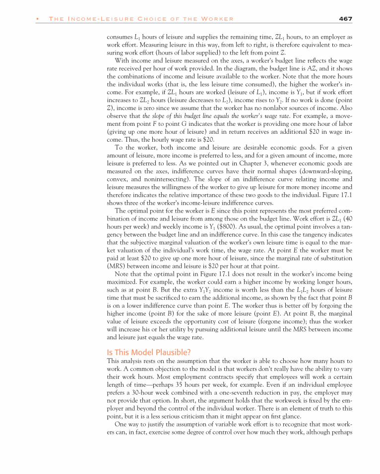
This analysis utilizes the indifference curve–budget line technique developed in Chapters3 and 4 for the analysis of consumer choice. In Figure 17.1, the vertical axis measures the in-dividual worker’s total weekly income, and the horizontal axis, from left to right, measuresthe worker’s leisure time. The term leisure refers to the portion of the worker’s time whenhe or she is not receiving compensation by an employer. Any worker has 168 hours a weekavailable, 24 hours a day, 7 days a week. We divide this time into two mutually exclusivecategories, work and leisure. Working time plus leisure time per week must equal 168 hours.In Figure 17.1, Z is the total time available, and the point L1 indicates that the individual

T

Weeklyincome

A

B

E

GF

U3

U2

U1

0

$201 hr.

L2 L1(128)

Z(168 hoursper week)

Leisure

Leisure

Work

Y2

$800 = Y1

Figure 17.1

leisurethe portion of a worker’stime when he or she is notreceiving compensationfrom an employer

Figure 17.1

Income-Leisure Choice of the WorkerMeasuring leisure from left to right is thesame as measuring hours worked fromright to left from point Z. The budget line AZ has a slope equal to the hourly wagerate. The optimal point is E, with theindividual working ZL1 hours and earning$800 per week.

• The Income-Leisure Choice of the Worker 467

consumes L1 hours of leisure and supplies the remaining time, ZL1 hours, to an employer aswork effort. Measuring leisure in this way, from left to right, is therefore equivalent to mea-suring work effort (hours of labor supplied) to the left from point Z.

With income and leisure measured on the axes, a worker’s budget line reflects the wagerate received per hour of work provided. In the diagram, the budget line is AZ, and it showsthe combinations of income and leisure available to the worker. Note that the more hoursthe individual works (that is, the less leisure time consumed), the higher the worker’s in-come. For example, if ZL1 hours are worked (leisure of L1), income is Y1, but if work effortincreases to ZL2 hours (leisure decreases to L2), income rises to Y2. If no work is done (pointZ), income is zero since we assume that the worker has no nonlabor sources of income. Alsoobserve that the slope of this budget line equals the worker’s wage rate. For example, a move-ment from point F to point G indicates that the worker is providing one more hour of labor(giving up one more hour of leisure) and in return receives an additional $20 in wage in-come. Thus, the hourly wage rate is $20.

To the worker, both income and leisure are desirable economic goods. For a givenamount of leisure, more income is preferred to less, and for a given amount of income, moreleisure is preferred to less. As we pointed out in Chapter 3, whenever economic goods aremeasured on the axes, indifference curves have their normal shapes (downward-sloping,convex, and nonintersecting). The slope of an indifference curve relating income andleisure measures the willingness of the worker to give up leisure for more money income andtherefore indicates the relative importance of these two goods to the individual. Figure 17.1shows three of the worker’s income-leisure indifference curves.

The optimal point for the worker is E since this point represents the most preferred com-bination of income and leisure from among those on the budget line. Work effort is ZL1 (40hours per week) and weekly income is Y1 ($800). As usual, the optimal point involves a tan-gency between the budget line and an indifference curve. In this case the tangency indicatesthat the subjective marginal valuation of the worker’s own leisure time is equal to the mar-ket valuation of the individual’s work time, the wage rate. At point E the worker must bepaid at least $20 to give up one more hour of leisure, since the marginal rate of substitution(MRS) between income and leisure is $20 per hour at that point.

Note that the optimal point in Figure 17.1 does not result in the worker’s income beingmaximized. For example, the worker could earn a higher income by working longer hours,such as at point B. But the extra Y1Y2 income is worth less than the L1L2 hours of leisuretime that must be sacrificed to earn the additional income, as shown by the fact that point Bis on a lower indifference curve than point E. The worker thus is better off by forgoing thehigher income (point B) for the sake of more leisure (point E). At point B, the marginalvalue of leisure exceeds the opportunity cost of leisure (forgone income); thus the workerwill increase his or her utility by pursuing additional leisure until the MRS between incomeand leisure just equals the wage rate.

Is This Model Plausible?This analysis rests on the assumption that the worker is able to choose how many hours towork. A common objection to the model is that workers don’t really have the ability to varytheir work hours. Most employment contracts specify that employees will work a certainlength of time—perhaps 35 hours per week, for example. Even if an individual employeeprefers a 30-hour week combined with a one-seventh reduction in pay, the employer maynot provide that option. In short, the argument holds that the workweek is fixed by the em-ployer and beyond the control of the individual worker. There is an element of truth to thispoint, but it is a less serious criticism than it might appear on first glance.

One way to justify the assumption of variable work effort is to recognize that most work-ers can, in fact, exercise some degree of control over how much they work, although perhaps


not on a daily or weekly basis. Overtime, vacation leave, leaves without pay, moonlighting,sick leave, and early retirement are options available to many workers. At a more basiclevel, each person has a wide range of options in selecting a job in the first place. Some jobsentail long hours, some short, and some permit considerable variation in work effort. For ex-ample, it is not unusual for entrepreneurs to average 80-plus hours of work per week in start-up firms striving to bring new products to market. Many of the same entrepreneurs could optfor less demanding jobs in the nonprofit, public, or private sectors (at established firms, forexample) that, while requiring fewer hours of work per week, are associated with less promis-ing financial rewards.

Another justification for the variable work effort assumption is that at a more fundamen-tal level the analysis may still be valid for many purposes, even if it is impossible for a workerto vary his or her workweek even slightly. Although the employer fixes the workweek, con-sider the economic factors that determine the level at which it is set. Employers are profitmaximizers, and it is therefore in their interest to cater to the preferences of workers, just asthey are led by profit motives to cater to the preferences of consumers. If a firm’s employeesprefer a 30-hour workweek, but the firm requires them to work 35 hours, it will lose workersto other firms that do a better job of satisfying the employees’ preferences. Competition forworkers thus leads firms to set workweeks that correspond to worker preferences. So, the as-sumption that workers can choose how much they will work should yield a reasonably cor-rect analysis, although it does not precisely describe reality.

One qualification should be mentioned. Employers have an incentive to cater to workers’preferences on average, but not necessarily to each employee’s preferences. The technologyof production requires most firms to have a common workweek for all employees (though itcan, and does, differ among firms). A fixed workweek means that workers with preferencesdifferent from the group average will not like the workweek schedule. Thus, our model maynot be strictly accurate for any specific worker, but it does provide a basis for analyzing workeffort decisions involving groups of workers.

17.2 The Supply of Hours of Work

Will workers work longer hours at a higher wage rate? The work-leisure choice model canhelp answer this question. Figure 17.2 examines the effect of a higher wage rate for a partic-ular worker. When the hourly wage rate is $20, the budget line is AZ, and the worker’s pre-ferred point is E with ZL1 work hours supplied. Remember that we measure work effort fromright to left in the diagram. If the hourly wage rate rises to $25, the budget line rotates aboutpoint Z and becomes steeper. The new budget line is A�Z with a slope of $25 per hour. Notethat at the higher wage rate income is greater for any level of work effort. Given the specificpreferences of this worker, when confronted with the higher wage rate, the new optimalpoint E� involves an increase in hours of work, from ZL1 to ZL2.

Does a higher wage always lead a worker to work more? The answer is no, and we can seewhy by considering the income and substitution effects associated with a change in thewage.

The substitution effect of a higher wage rate encourages a worker to supply more hours oflabor. When the hourly wage rate rises from $20 to $25, the sacrifice for leisure consumptionis greater, since each hour of leisure now means giving up $25 in income instead of $20.Since leisure has become more costly in terms of income lost, the worker is encouraged tosubstitute away from leisure toward income—that is, to work more.

An income effect is also associated with a higher wage rate but has an opposite result onwork effort from the substitution effect. A wage increase makes the individual better off,permitting the worker to reach a higher indifference curve. A higher real income tends to

• The Supply of Hours of Work 469

increase the consumption of all normal goods, and leisure for most people is a normal good.The income effect of a wage rate increase thus encourages the consumption of leisure andleads the worker to work less. Because of the higher wage, the worker can afford to work less;it is possible to work fewer hours and still achieve a higher money income than before thewage increase.

Figure 17.2 shows that the substitution effect of a higher wage rate encourages more work, and theincome effect encourages less work. The hypothetical budget line HH� is drawn tangent to theworker’s original indifference curve U1. Its slope reflects the higher wage rate of $25. The substi-tution effect is shown as the movement along U1 from E to E1. Because leisure has become morecostly, the worker consumes less, and work effort increases from ZL1 to ZL3. The income effect isshown as the movement from E1 to E� when we allow the individual to move from the HH�budget line to the parallel A�Z budget line, reflecting the increase in real income associatedwith the rise in the wage rate. Since leisure is a normal good, the income effect involves moreleisure, from L3 to L2, which is the same as saying it encourages less work—that is, ZL2 instead ofZL3. The total effect of the higher wage rate is the sum of the income and substitution effects.Although these effects operate in opposite directions, in this case the substitution effect islarger, so the total effect is an increase in work hours from ZL1 to ZL2.

Is a Backward-Bending Labor Supply Curve Possible?For the worker whose preferences are depicted in Figure 17.2, the supply curve of workhours slopes upward, at least between wage rates of $20 and $25, since a higher wage leadsto a greater quantity of labor supplied. This outcome need not always be the case, however.The income effect of a higher wage may be larger than the substitution effect, resulting in a

E1

Weeklyincome

$25

A′

E′

E

U2

U1

H

A

0

1 hr.

$251 hr.

$201 hr.

I

S

TE

H′ ZL3 L2 L1 Leisure

Figure 17.2Figure 17.2

Worker’s Response to a Change in the Wage RateA higher wage rate pivots the budget line from AZ to A�Zand work effort increases from ZL1 to ZL2. We show theincome and substitution effects of the change in thewage rate by using the hypothetical budget line HH� thatis parallel to the A�Z budget line but just tangent to theinitial indifference curve U1. The substitution effect, L1L3,involves more work, but the income effect, L3L2, involvesless. In this case the combined effect implies greaterwork effort at the higher wage rate.


reduction in work hours at higher pay. The intuition behind such an alternative outcome isstraightforward. Beyond some point individuals may prefer to work a little less, take sometime off, and enjoy the higher income made possible by a higher salary. For example, 30hours a week at a wage of $25 per hour means more income and more leisure time withwhich to enjoy the income when compared to 40 hours at a wage of $5 per hour.

Figure 17.3a shows an individual who will choose to work longer hours when the wageincreases from $20 to $25 but will then decide to work somewhat less when the wage risesagain. When the wage increases from $20 to $25, work hours increase from ZL1 to ZL2, butat a wage of $30, hours worked falls to ZL3. (We have not separated the income and substi-tution effects in the diagram, but you may wish to do so.) Figure 17.3b shows the same infor-mation plotted as a labor supply curve of weekly work hours. The supply curve slopes upwardbetween wage rates of $20 and $25 but bends backward as the wage rate rises further.

A supply curve of work hours can thus be backward-bending beyond some wage rate.Note that a backward-bending labor supply curve does not depend on an unusual set of cir-cumstances, as does an upward-sloping demand curve; rather, it just requires that the normalincome effect of a higher wage rate exceed the substitution effect. Leisure is a normal good, so theincome and substitution effects always work in opposing directions in the case of a laborsupply curve because the worker is a seller of labor services. A rise in the price of somethingan individual sells (such as labor services) has a positive effect on the individual’s incomeand thus leads to greater consumption of all normal goods, including leisure. (In contrast,when the price of something you purchase as a buyer increases, the effect on your income isnegative. The negative income effect reinforces, rather than counteracts, the substitution

Weeklyincome

A′′

E′′

E

E′

A′

A

L2 L3

U3U2

U1

L1 Z

(a)

Leisure0

1 hr.

$30

1 hr.

$25

1 hr.

$20

Hourlywage

E′′

S

E

E′

$30

$25

$20

ZL1

ZL3

ZL2

(b)

Labor0

An Individual Worker’s Weekly Supply of Work(a) An individual’s choices of how much to work at three different wage rates arerepresented by E, E�, and E �. (b) These labor supply choices are plotted as the supplycurve of weekly work hours. When the income effect exceeds the substitution effect, thesupply curve becomes backward-bending.


• The General Level of Wage Rates 471

effect for a normal good.) Moreover, the income effect of a change in pay is likely to be largerelative to the substitution effect since most income derives from providing labor.

The Market Supply CurveTo go from an individual’s supply curve of work hours to the market supply curve, we needonly horizontally sum the responses of all workers competing in a given labor market. Thus,the market supply curve can also slope upward, bend backward, or show a combination ofthe two, as shown in Figure 17.3b. Theoretical considerations alone do not permit us to pre-dict the exact shape of the market supply curve. Empirical evidence, however, suggests thatit slopes upward (at least for wage rates near present levels), with an elasticity somewherebetween 0.1 and 0.3.1 An elasticity of 0.1 means that a 10 percent increase in the wage rateincreases the quantity of labor supplied by 1 percent. Such an inelastic supply curve slopesupward and is almost vertical.

A highly inelastic aggregate supply curve, as suggested by the empirical evidence, appearsplausible. Casual observation suggests that the amount of time most people work stays thesame over moderate periods of time despite changes in wage rates. If individual supplycurves were sharply upward-sloping or backward-bending, we would see substantial changesin individuals’ work hours in jobs where market forces have produced large wage ratechanges. Work hours per worker in most jobs seem to be quite stable over time, suggestingthat the effect of wage rate changes on work hours is not pronounced. This result does notmean that people are completely unresponsive to wage rate changes, only that the responsesthat occur are modest.

When should we use the aggregate labor supply curve? In the preceding chapter we em-phasized that the labor supply curve to a particular industry or occupation is likely to slope up-ward and be quite elastic. We must distinguish that type of labor supply curve, however,from the one discussed here. In looking at the supply to an industry or occupation, we seethat the quantity of labor services can increase sharply with a rise in the wage rate in thatjob, but the increase results mainly from an influx of workers from other jobs or industriesand not from a change in work hours of current workers. The supply curve of labor to a spe-cific job or industry therefore depends mainly on how the number of workers varies withwage rates in those specific occupations.

The aggregate labor supply curve is used in cases when the movement of workers betweenjobs is not likely to be significant but the possible change in the hours supplied by workers intheir current jobs is. For example, how would a 10 percent increase in all wage rates affectthe total quantity of labor supplied? Since all jobs will pay proportionately more, people willhave little incentive to change jobs. The only way the total labor supply will increase, there-fore, is if people work longer hours (which includes the possibility that some people willenter the labor force for the first time at the higher wage rate). For this type of aggregateanalysis, which involves the total quantity of labor supplied across all industries, the marketsupply curve of work hours is appropriate. We discuss an example using this supply curve inthe next section and offer more examples in Chapter 18.

17.3 The General Level of Wage Rates

In analyzing the determination of wage rates, it is convenient to divide the subject into twoparts: determination of the general level of wage rates and consideration of why they differamong jobs. In this section we focus on the factors that influence the level of real wages, or

1For a representative survey of the empirical evidence see U.S. Congressional Budget Office, An Analysis of theRoth-Kemp Tax Cut Proposal (Washington, D.C.: U.S. Government Printing Office, 1978).


the average wage rate; we defer until the next section a discussion of the factors that cause avariation in wage rates around the average.

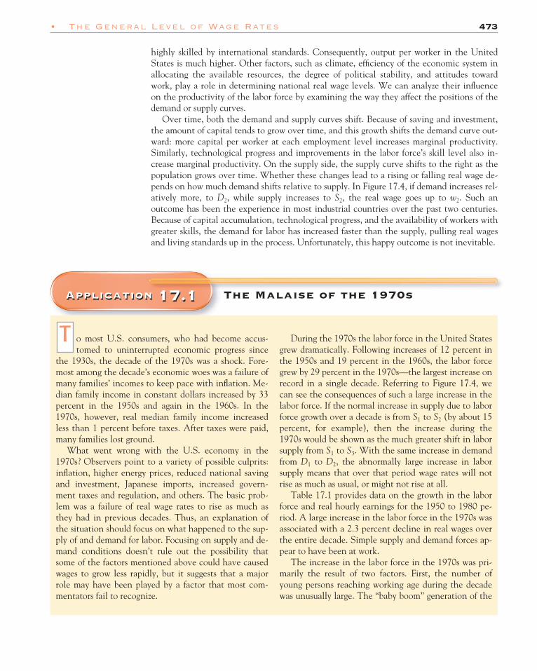
Supply and demand are still the applicable concepts for investigating the level of wagerates. The supply curve of labor indicates the total quantity of labor supplied by all personsat various wage levels. The appropriate supply concept is therefore the aggregate supplycurve of work hours discussed in the previous section. This supply curve is probably quite in-elastic, like curve S1 in Figure 17.4.

The aggregate demand curve for labor reflects the marginal productivity of labor to the economyas a whole. Indeed, it is convenient to think of the wage rate as being paid in units of na-tional output (each unit composed of the combination of goods consumed by the averageperson) to emphasize that we are dealing with the level of real wage rates. In constructingthe demand curve relevant for a particular time period, the following factors are held con-stant: capital (including land, buildings, and equipment), technology, and the skills, knowl-edge, and health of the labor force. If these factors are fixed, an increase in the total quantityof labor is subject to the law of diminishing marginal returns. Consequently, the aggregatemarginal product curve slopes downward and is the aggregate demand curve for labor.

At any particular time, if the supply curve is S1 and the demand curve is D1 as in Figure17.4, then the (average) real wage rate is w1 and employment is L1. At the high degree of ag-gregation used in this analysis, the model is necessarily abstract and ignores a multitude offactors that could influence the positions of the demand or supply curves. Yet it highlightsthe importance of the productivity of labor in determining the level of wages. National out-put and national income are two sides of the same coin, and with labor receiving about 75percent of national income (output), it is clear that the factors that determine the outputlevel produced from a given quantity of labor play a central role in the analysis. These fac-tors are primarily (but not exclusively) technology, the skill level of the labor force, and theamounts of other inputs, which in this example we refer to as capital.

This concept explains why real wages are so much higher in the United States than inless developed countries: the (marginal) productivity of labor is greater. Marginal productiv-ity is higher because of the factors determining the position of the demand curve: capital,technology, and skills. In U.S. manufacturing industries the amount of capital per worker isabout $125,000, contributing to high average and marginal productivity of labor. Techno-logical knowledge is superior in this country, and the U.S. labor force is well educated and

Wage

w2

w1

0 L1

D1

D2

S1S2 S3

L2 Labor


Determination of the General Wage LevelThe aggregate demand curve for labor interacts with theaggregate supply curve to determine the general wage level. Overtime, normally both supply and demand increase. If demandincreases faster than supply, wage rates tend to rise over time.

Application 17.1

o most U.S. consumers, who had become accus-tomed to uninterrupted economic progress since

the 1930s, the decade of the 1970s was a shock. Fore-most among the decade’s economic woes was a failure ofmany families’ incomes to keep pace with inflation. Me-dian family income in constant dollars increased by 33percent in the 1950s and again in the 1960s. In the1970s, however, real median family income increasedless than 1 percent before taxes. After taxes were paid,many families lost ground.

What went wrong with the U.S. economy in the1970s? Observers point to a variety of possible culprits:inflation, higher energy prices, reduced national savingand investment, Japanese imports, increased govern-ment taxes and regulation, and others. The basic prob-lem was a failure of real wage rates to rise as much asthey had in previous decades. Thus, an explanation ofthe situation should focus on what happened to the sup-ply of and demand for labor. Focusing on supply and de-mand conditions doesn’t rule out the possibility thatsome of the factors mentioned above could have causedwages to grow less rapidly, but it suggests that a majorrole may have been played by a factor that most com-mentators fail to recognize.

T During the 1970s the labor force in the United Statesgrew dramatically. Following increases of 12 percent inthe 1950s and 19 percent in the 1960s, the labor forcegrew by 29 percent in the 1970s—the largest increase onrecord in a single decade. Referring to Figure 17.4, wecan see the consequences of such a large increase in thelabor force. If the normal increase in supply due to laborforce growth over a decade is from S1 to S2 (by about 15percent, for example), then the increase during the1970s would be shown as the much greater shift in laborsupply from S1 to S3. With the same increase in demandfrom D1 to D2, the abnormally large increase in laborsupply means that over that period wage rates will notrise as much as usual, or might not rise at all.

Table 17.1 provides data on the growth in the laborforce and real hourly earnings for the 1950 to 1980 pe-riod. A large increase in the labor force in the 1970s wasassociated with a 2.3 percent decline in real wages overthe entire decade. Simple supply and demand forces ap-pear to have been at work.

The increase in the labor force in the 1970s was pri-marily the result of two factors. First, the number ofyoung persons reaching working age during the decadewas unusually large. The “baby boom” generation of the

• The General Level of Wage Rates 473

highly skilled by international standards. Consequently, output per worker in the UnitedStates is much higher. Other factors, such as climate, efficiency of the economic system inallocating the available resources, the degree of political stability, and attitudes towardwork, play a role in determining national real wage levels. We can analyze their influenceon the productivity of the labor force by examining the way they affect the positions of thedemand or supply curves.

Over time, both the demand and supply curves shift. Because of saving and investment,the amount of capital tends to grow over time, and this growth shifts the demand curve out-ward: more capital per worker at each employment level increases marginal productivity.Similarly, technological progress and improvements in the labor force’s skill level also in-crease marginal productivity. On the supply side, the supply curve shifts to the right as thepopulation grows over time. Whether these changes lead to a rising or falling real wage de-pends on how much demand shifts relative to supply. In Figure 17.4, if demand increases rel-atively more, to D2, while supply increases to S2, the real wage goes up to w2. Such anoutcome has been the experience in most industrial countries over the past two centuries.Because of capital accumulation, technological progress, and the availability of workers withgreater skills, the demand for labor has increased faster than the supply, pulling real wagesand living standards up in the process. Unfortunately, this happy outcome is not inevitable.

Application 17.1 The Malaise of the 1970s


17.4 Why Wages Differ

From the market forces that determine the general level of wage rates, we turn now to thequestion of why there is such wide variation in the wages received by different individuals.In Chapter 16, we explained why wage rates across firms or industries tend to equalize. Thatanalysis depended on the assumptions that workers were identical and that they evaluatedthe desirability of the jobs only in terms of the money wage rates. Dropping these assump-tions, as we must for a fuller understanding of labor markets, suggests that wage rates can dif-fer among jobs and among people employed in the same line of work. People are different inthe type of work they are both able and willing to perform, and these differences on the sup-ply side of labor markets produce differences in wage rates.

Perhaps the best way to see what is involved is to take a hypothetical, but plausible, ex-ample. Figure 17.5a shows the labor market for clerks, and Figure 17.5b shows the labor mar-ket for engineers. Under competitive conditions, the intersection of supply and demandcurves in each market yields a wage rate for engineers that is twice that for clerks. We sug-gest that these markets are in full equilibrium with no tendency for the wage rates to equal-

1950s had grown up. Second, the share of females in thelabor force increased from 43 percent in 1970 to 52 per-cent in 1980. (The labor force participation rate of fe-males had never exceeded 40 percent before 1966.)Each of these factors was significant in itself, but to-gether they spelled an unusually large increase in laborsupply. Labor markets, however, adjusted to accommo-date this influx of workers, and employment increasedby millions more than it had in any previous decade.The relatively large shift in supply meant that wage ratesrose less than in previous decades.

What roles did inflation, energy prices, decreased sav-ing, and the other factors so frequently mentioned play inaffecting real wage rates? Several caused the demand forlabor to grow less rapidly than it had in previous decadesand thus reinforced the tendency for wage rates to risemore slowly. For example, a reduced rate of investment

and a higher price of oil—an input purchased in largequantities from other countries—both depressed the rateof increase in labor demand. Theory suggests, however,that some of the other factors frequently mentioned, likeinflation and higher imports of consumer goods fromJapan, would have little effect, since they do not signifi-cantly affect productivity. The exact quantitative contri-bution of each of these factors to the slowdown in thegrowth of real wages is an unresolved issue and has beenthe subject of some debate among economists.

The role of other factors notwithstanding, the mas-sive increase in the number of workers in the labor forceappears to have had a significant impact on real wagesduring the 1970s in the United States. Moreover, thesupply–demand model appears to offer the correct ap-proach to the question of what caused the decline inreal wages during this period.

Table 17.1 Size of Labor force and Wage Rates, 1950–1980

Labor Increase over Index of Real Increase overForce Previous Period Hourly Earnings Previous Period

(Millions) (Percentage) (1971 = 100) (Percentage)

1950 62.2 – 64.0 –1960 69.6 11.9 81.4 27.21970 82.8 19.0 95.7 17.61980 106.9 29.1 93.5 �2.3

Source: Economic Report of the President, 1982.

• Why Wages Differ 475

ize. Is this result possible, and if so, why? Why don’t some clerks leave their low-paying jobsand become engineers, a movement that would tend to equalize wage rates in the two occu-pations? Why don’t employers of engineers seek out workers presently employed as clerksand offer them engineering jobs at better pay (but at wage rates slightly below wE) sincetheir demand curve indicates they would be willing to hire more engineers at a lower wage?

Thinking about these questions suggests several possible answers. First, workers currentlyemployed as clerks may prefer their jobs despite the financial difference; that is, they don’twant to work as engineers. Second, acquiring the skills to become an engineer may have asignificant cost. The wage for engineers may not be sufficiently high to compensate clerksfor the training costs they would have to bear to become engineers. Third, even if therewere no training costs, clerks may not have the aptitude for science and mathematics neces-sary to work as engineers.

Training costs as well as differences in workers’ abilities and/or preferences for particularjobs can lead to equilibrium differences in wage rates among persons and jobs; there is no ten-dency toward adjustments that would wipe out wage differentials due to such factors. Nowlet’s take a somewhat more detailed look at these factors.

Compensating Wage DifferentialsMonetary compensation is not the only factor, and sometimes not even the most importantfactor, influencing individuals’ job choices. People routinely make decisions to take jobspaying less in monetary terms than they might earn elsewhere. Many academic economists,for example, could earn 50 percent more working for government or industry but choose toremain in a scholarly environment. Similarly, some people might agree to work at the samejob for less money if they could live in the Sun Belt instead of the Northeast.

Wage

wC

0 LC

D

S

Labor servicesof clerks

(a)

Wage

wE

0 LE

D

S

Labor servicesof engineers

(b)

Equilibrium Wage Differences(a) The labor market for clerks results in wage rate wC. (b) The labor market for engineersresults in wage rate wE. Although the wage rate for engineers is higher, there is notendency for these wage rates to equalize: they are equilibrium wage differences.


Application 17.2

ach year hundreds of “jumpers” or “glow boys” arehired by public utilities to fix steel pipes in aging

power plants.2 The jumpers work for only 10 minutes ata time and are paid the equivalent of 12 hours of averagemaintenance wages in addition to free travel and perdiems. The only catch is the job site: the pipes are lo-cated inside nuclear power plants where radiation is so

E intense that a jumper can stay for only a limited periodof time before, in industry parlance, “burning out.” Themaximum amount of radioactivity to which a jumpermay be exposed is 5,000 millirems per year (the equiva-lent of 250 chest X-rays). The Nuclear Regulatory Com-mission, which sets the limit, estimates that if workersare exposed to even that level for 30 years, 5 percentwill die of cancer as a result. The high pay earned byjumpers thus illustrates a compensating wage differen-tial: riskier jobs pay more.


When workers view some jobs as intrinsically more attractive than others, the forces ofsupply and demand produce differences in the wages paid. These differences are calledcompensating wage differentials because the less attractive jobs must pay more to equalizethe real (monetary and nonmonetary) advantages of employment across jobs.

We can illustrate the implications of differences in job attractiveness. Suppose a certainnumber of potential workers are identical in their abilities to work as police officers or firefighters. At equal wages, they would all prefer to be fire fighters, perhaps because they thinkpolice work is a thankless task. Only if the police wage is at least 25 percent higher than thefire fighting wage will they choose to enter the police force. If market conditions determinewages, then wages for police officers will be 25 percent higher than those for fire fighters.Only then would the real wage, in the eyes of the workers, be the same for the two jobs.

Differences in money wages are necessary to equate the quantity of labor supplied and de-manded in different occupations when the nonmonetary attractiveness of jobs differs. Somecities have ignored this fact and set the same wages for police officers and fire fighters. Theoutcome? A surplus of fire fighter recruits and a shortage of police force applicants.

Application 17.2 Twelve Hours’ Pay for Ten Minutes’ Work

2“Ten Minutes’ Work for 12 Hours’ Pay? What’s the Catch?,” WallStreet Journal, October 12, 1983, pp. 1 and 21.

Differences in Human Capital InvestmentOur ability to perform useful services can be augmented by training, education, and experi-ence. People can become more productive workers, and more productive workers receivehigher wage rates. The process by which people augment their earning capacity is sometimescalled human capital investment. In these terms, human beings are viewed as capable ofgenerating a flow of productive services over time, much as capital assets can. When theybear the costs of training or education themselves, they are investing in their own earningcapacity by attempting to increase the productive services they can provide as workers.

Education and training are much like other investments. Initially, people incur costs. Forcollege students, for example, the explicit and implicit costs include tuition, fees, and for-gone income. The payoff to the investment comes several years later; then, you find out howprofitable the investment was. If earning capacity has increased sufficiently, the higher earn-ings in later years cover the initial investment cost. No student needs to be told that thisform of investment, like many others, is risky.

compensatingwagedifferentialsdifferences in wages paidthat are created by theforces of supply anddemand when workersview some jobs asintrinsically moreattractive than others

human capitalinvestmentthe process by whichpeople augment theirearning capacity

Application 17.3

lthough investing in a college education involvessome risk, the average return, net of any costs, ap-

pears to be greater than ever.3 As of 2000, according tothe U.S. Census Bureau, workers with a college degreemade 80 percent more than workers with only a highschool diploma. As recently as 1988, college degreeholders made just 48 percent more than workers withonly a high school diploma. Researchers estimate that as

A much as 30 to 50 percent of the relative wage gainsmade by college graduates over the past decade reflectthe spread of computer technology and the fact thatcollege-educated workers tend to be more proficient atusing computers than their non-college-educated coun-terparts.

The Census Bureau does not track the median an-nual income for holders of an MBA degree. Accordingto Business Week, however, pursuing an MBA at one ofthe top 30 schools appears to be a profitable investment.Graduates of these schools landed jobs with medianstarting salaries of $111,100 in 2002. Prior to enrollingin an MBA program, the same graduates had medianearnings of $53,700 per year.

• Why Wages Differ 477

Jobs requiring large human capital investments tend to pay higher wages. The reason issimple: if the wages weren’t higher, few people would be willing to incur the training costs.The higher wages associated with highly skilled work are, in part, the returns on past invest-ments in human capital. According to this view, it is no accident that college graduates onaverage earn more than high school graduates or that neurosurgeons earn more than typists.

In terms of our labor supply–demand model, the supply curve tells us that the amount oflabor supplied to jobs requiring large investments in human capital will be forthcoming onlyat higher wage rates. Thus, in Figure 17.5, the supply curve of engineers is positioned higher(vertically) than the supply curve for clerks.

Application 17.3 The Returns to Investing in a BA and an MBA

3This application is based on “Advanced Degrees Result in HigherEarnings,” Chronicle.com, July 18, 2002; “The Payoff from ComputerSkills,” Business Week, November 3, 1997, p. 30; and “The Best Busi-ness Schools,” Business Week, October 21, 2002.

Differences in AbilityWorkers’ productive capacities depend not only on their training and experience (humancapital investment) but also on certain inherited traits. The relative importance of thesetwo factors is greatly disputed. For years people have debated whether genetic or environ-mental factors are more important in explaining IQs. There is no doubt, however, that in-herited traits play a significant role in determining what we are capable of doing. No amountof training could turn all of us into nuclear physicists, basketball stars, entertainers, models,politicians, or business executives. People differ in strength, stamina, height, mental ability,physical attractiveness, motivation, creativity, and numerous other traits. These traits, orthe lack of them, influence the work we are capable of accomplishing.

Similarly, possessing abilities that are scarce is no guarantee of a high wage. For exam-ple, the ability to wiggle your ears may be uncommon but is unlikely to generate a high in-come. What matters is the supply of persons with abilities required to perform certain jobsrelative to the demand for their services. If consumers were unwilling to pay to watch ath-letes throw balls through a hoop, being able to slam-dunk in 12 different ways would notcommand a million-dollar salary. Obviously, then, some human abilities are in limited sup-ply relative to demand, and, as a result, those endowed with such abilities can commandhigher wages.

Application 17.4

recent study indicates that beauty tends to be re-warded by the labor market.4 Using interviewers’

ratings of respondents’ physical appearance, the studyfound that good-looking people earn higher wages thanaverage-looking people, who in turn earn higher wages

A than plain-looking people. The wage premium paid bythe labor market for good looks is roughly 5 to 10 per-cent relative to average looks and 10 to 20 percent rela-tive to plain (below average) looks. The wage premiumfor beauty holds across occupations and for both womenand men (if anything, the premium is larger for menthan for women). Thus, contrary to the well-known say-ing, it’s not just what’s on the inside that counts whendetermining the wages earned by different workers.


Application 17.4 What’s on the Outside Also Counts

4Daniel S. Hamermesh and Jeff E. Biddle, “Beauty and the Labor Mar-ket,” American Economic Review, 84 No. 5 (December 1994), pp.1174–1194.

17.5 Economic Rent

In ordinary usage, rent refers to payments made to lease the services of land, apartments,equipment, or other durable assets. Economists use the term differently. Economic rent is de-fined as that portion of the payment to an input supplier in excess of the minimum amountnecessary to retain the input in its present use. The economic rent accruing to suppliers ininput markets is thus analogous to the concept of producer surplus in output markets.

In the history of economics, the term rent was originally associated with the payments tolandowners for the services of their land. To see why, let’s suppose that the supply of land isfixed, so its supply curve is vertical. (This assumption is a slight exaggeration since the sup-ply of usable land is not absolutely fixed; without care land can erode, become overgrown, orlose its fertility.) A vertical supply curve means that landowners will place the same quan-tity on the market regardless of its price. Even at a zero price the same amount of land wouldbe available. Thus, the minimum payment necessary to retain land in use is zero, and any ac-tual payment above zero exceeds the minimum amount necessary to call forth the supply.All the payments to landowners therefore satisfy the definition of economic rent.

Figure 17.6 illustrates this point. The vertical supply curve of land interacts with the de-mand curve to determine the equilibrium price. The price and quantity are specified permonth to indicate that we are concerned not with the sale price of the land but rather withthe price for the services yielded by the use of land. The shaded area indicates the monthlyincome received by land suppliers.5 The shaded area also equals the economic rent receivedby landowners, because all payments for the services of land exceed the (zero) amount nec-essary to have a supply of Q. The position of the demand curve determines the amount ofeconomic rent. If demand increases, the price of land services goes up and the shaded areabecomes larger, but the larger shaded area would still be all rent.

Because nineteenth-century economists regarded the supply of land as fixed, they viewedpayments to landowners as economic rent. Today economists recognize that suppliers ofother inputs may receive economic rent as well. The prices received by the owners of any

5In practice, owners often do not receive the income from the use of their land in monetary form. Homeowners, forexample, secure the services of the land on which their houses rest. Since they own the land, the income from itsuse is in the form of these services directly received, but these services have a monetary value determined by supplyand demand.

economic rentthat portion of thepayment to an inputsupplier in excess of theminimum amountnecessary to retain theinput in its present use

• Economic Rent 479

input in fixed supply are entirely rent, and part of the prices received by inputs with upward-sloping supply curves are also rent. Consider the supply of university professors. For clarity,let’s examine the discrete case involving a small number of persons. The supply curve isthen the step-like relationship in Figure 17.7. In equilibrium, five professors are working: in-dividuals A, B, C, D, and E. We assume that they are identically productive as professors butnot identical in their abilities to perform other jobs.

Individual A will be willing to work as a professor if paid area A1. Even at a very low wagehe will opt for the academic life because his next best employment opportunity is as a dish-washer, where he would earn very little. Individual B has a better alternative; she could sellused cars. She will work in academe if she receives at least area B1. And so we progress upthe supply curve. The supply curve slopes upward because to attract more people, collegesmust bid them away from increasingly more attractive alternative employments.

Price

P

S

0 Q Land

D

Figure 17.6

Wage

w

0 2 3 4 5 6 College professors1

S

D

A2

B2

C2

D2

A1

B1

C1

D1

E1

Figure 17.7

Figure 17.6

Economic Rent with a Vertical Supply CurveWhen the input supply curve is vertical, the entire remuneration ofthe input (the shaded area) represents economic rent, since thesame quantity would be available even at a zero price.

Figure 17.7

Economic Rent with an Upward-Sloping Supply CurveWith an upward-sloping input supply curve, part of thepayment to input owners represents rent. In this caseindividuals A, B, C, and D receive rent equal to areas A2, B2, C2, and D2, respectively.


When this labor market is in competitive equilibrium, individuals A to E are paid a wageof w. A wage of w means that individual A receives an amount greater than the minimumnecessary to induce him to work as a professor. Recall that the minimum amount is area A1,but he is being paid A1 plus A2, so A2 represents an economic rent. Individuals B, C, D, andE receive rents equal to B2, C2, D2, and zero, respectively. Individual E is paid just enough toinduce her to supply her services as a professor. If the wage were any lower, she would workelsewhere, so none of her earnings represents rent.

In this example, part of the earnings of professors (except for E) are economic rent, andthe remainder is the payment required to keep the individuals from leaving their academicjobs and working elsewhere. The total rent received is the sum of the colored areas. When-ever the supply curve of any input slopes upward, part of the payment to inputs will be rent,as in this example. The more inelastic the supply curve, the larger the rent as a fraction ofthe total payment to an input. In the extreme case of perfectly inelastic supply (Figure 17.6),all the payment represents rent.

17.6 Monopoly Power in Input Markets: The Case of Unions

In Chapter 16 we examined the hiring of inputs by firms operating in either perfectlycompetitive or monopoly output markets. We also explored the effects of buying ormonopsony power in input markets. We did not, however, address selling or monopolypower in input markets. We do so here by focusing on labor unions. If effectively orga-nized, labor unions are an input’s sole supplier of the labor services of the union’s mem-bers and thus have some influence over the wages union members are paid. Much as amonopolist in a product market seeks a price and an output level so as to maximize profit,a labor union seeks a wage and employment level so as to maximize the economic rent ac-cruing to its members.

Consider Figure 17.8, where the demand and supply of labor to a market are given by thecurves D and S. These curves depict the quantity of labor services demanded and supplied,respectively, at various possible wage rates absent any monopsony or monopoly power.Under competitive conditions, LC workers are hired at a wage rate of wC.

Now suppose that workers unionize and effectively cartelize the supply side of the marketdepicted in Figure 17.8. By organizing, the union’s members acquire monopoly power andcan exercise that power by selecting any wage–employment level combination on the de-mand curve for labor services confronting the union.6

What point on the demand curve for their services should a union’s members select ifthey are interested in maximizing their economic rent? Analogous to the case of monop-oly power in output markets, the union needs to take into account the marginal revenuecurve, MR, associated with the demand curve for its services. The marginal revenue curverepresents the additional wages earned by the union membership as a whole when an in-cremental worker is hired. The marginal revenue curve lies below the demand curve at allemployment levels since the hiring of an additional worker requires the union to lowerthe wage level paid to all previously employed workers. The reduced payments to previ-ously employed workers must be subtracted from the wage earned by the incrementalworker (the height of the demand curve) to derive the additional wages earned by the

6For ease of discussion we assume that the union cannot engage in price discrimination, securing different wages forits various members. When an input supplier can price discriminate, an analysis analogous to the one presented inChapter 12 on price discrimination in output markets is applicable.

• Monopoly Power in Input Markets: The Case of Unions 481

Wage

wU

wC

F

0 LU LC Workers

D

S

A

E

B

MR

The Effect of an Input Market MonopolyAn effectively organized union represents a monopoly in the market for labor services. Tomaximize economic rent, the union selects the employment level where the marginalrevenue, in terms of additions to the union’s wage bill, from having an additional workerhired (the height of the MR curve) equals the opportunity cost needed to induce theworker to work (the height of the S curve). The union employment level is LU at a wagerate of wU. The economic rent accruing to the union equals area wUABF.

union as a whole (the height of the marginal revenue curve) when the incrementalworker is hired.

To maximize economic rent, the union compares the additional wages resulting from thehiring of another worker (MR) with the bare minimum the worker needs to be paid to workin this market—the worker’s opportunity cost. The height of the supply curve represents thebare minimum that needs to be paid to induce an incremental worker to work at variouspossible total employment levels and thus is effectively the union’s marginal cost curve.Much as profit in an output market is maximized by setting marginal revenue equal to mar-ginal cost, the economic rent earned by a labor union’s members is maximized by selectingan employment level, LU, where MR intersects S in Figure 17.8. Up to LU, every worker con-tributes more to the union’s total wage payments than it costs to induce him or her to work.The wage rate set by the union-monopoly is wU and the economic rent accruing to the



union membership as a whole is depicted by area wUABF—the excess of the wage rate overworkers’ opportunity costs from zero to the quantity of labor services sold, LU, by the union-monopoly.

Note that in Figure 17.8 fewer workers end up being employed as a result of the unionthan under competitive conditions. This is because the union is presumed to be interestedin maximizing the economic rent accruing to its membership rather than the number ofworkers having jobs. The economic rent from the monopoly outcome of LU and wU (areawUABF) exceeds the economic rent associated with the competitive outcome of LC and wC

(area wCEF).By restricting output in the market for labor and raising the prevailing wage rate, the

union illustrated in Figure 17.8 produces a deadweight loss similar to the one resulting frommonopoly in output markets. Triangular area AEB is the deadweight loss associated with thelabor union. This can be seen by noting that in order to maximize economic rent, the unionrestricts labor employment to LU from LC. Each worker between LU and LC can generatemore in terms of the value of output produced (the height of the D curve) than it costs toinduce the worker to work (the height of the S curve). These potential net gains are not re-alized, however, because a labor union interested in maximizing economic rent does notcare about the total value of the output produced by an incremental worker (the height ofthe demand curve). Rather, such a union cares about the incremental worker’s contributionto the union’s total wage bill (the height of the MR curve).

While acknowledging the potential deadweight loss associated with unions, some econ-omists have argued for a more benign evaluation of their role since they may be organizedto counteract monopsony power possessed by input-buying firms.7 For example, in thisview, the United Auto Workers union arose out of the need to protect workers’ rights andwages from the actions of the “Big Three” automobile companies. Furthermore, to the ex-tent that unions set up effective grievance procedures and give workers a “voice” with theiremployers, they may actually make workers more satisfied and productive on the job (theheight of the labor demand curve shifts upward if workers become more productive, all elseequal).

There is some empirical evidence that, controlling for other factors, union workers notonly receive higher wages but also are more productive than nonunion workers. Most econ-omists, however, are skeptical that unions actually improve workers’ productivity. Onewould expect the value of the final output produced by an additional worker to increase thefewer the number of workers hired. Fewer workers have more of the other, nonlabor inputsto share between themselves and thus, if the law of diminishing returns holds, have highermarginal products.

In Figure 17.8, for example, the height of the labor demand curve reflects the value ofthe final output produced by an incremental worker and could be used as a measure ofworker productivity. According to such a measure, workers are more productive at theunion employment level of LU than at the competitive level of LC. This does not imply,however, that the union has made each worker more productive. The height of the de-mand curve at an employment level LU is just as high under a union-monopoly as it is withperfect competition. Once again it is important to distinguish between a movement alonga given demand curve (in this case a labor demand curve) and a potential shift of the entiredemand curve.

7See, for example “Unions Need Not Apply,” New York Times, July 26, 1999, pp. C1 and C14; and Richard B.Freeman and James L. Medoff, What Do Unions Do? (New York: Basic Books, 1984).

Application 17.5

abor unions in the United States have undergonedramatic membership changes over the past few

decades.8 In the private sector, the percentage of nona-gricultural wage and salary workers who are union mem-bers has plummeted from 38 percent in the early 1950sto 9 percent in the late 1990s. By contrast, over thesame time period, public sector union membership hasskyrocketed from 10 to 37 percent.

What accounts for the different fortunes of privateand public sector unions in the United States over thepast few decades? Public sector unions have grown inrelative importance due to changes in labor laws favor-able to the unionization of government workers at alllevels of government throughout the 1960s and 1970s.Prior to the 1960s, collective bargaining by most gov-ernment workers was illegal.

In the private sector, the rapid growth of the hightechnology sector explains some of the overall declinein union membership in the United States. Only asmall fraction of the 5 million employees who work forcomputer semiconductor and software companies are

L unionized. This is due to demand for such workersgrowing much more quickly than the supply and com-panies promising generous salaries and stock options torecruit and retain workers—rewards that diminish therelative benefits workers could obtain through union-ization.

Furthermore, growing international competition incertain industries, such as automobile production, andthe enhanced competitiveness of other deregulated in-dustries, such as trucking and airlines, have made theoutput demand curves for firms operating in these indus-tries more price elastic. As we saw in the previous chap-ter, one of the factors that determines the elasticity ofdemand for an input (and hence the monopoly power ofsellers of that input) is the elasticity of the demand forthe final product produced by the input. For example,the monopoly power possessed by the United AutoWorkers has been lessened as American car manufactur-ers have faced growing foreign competition. In the1950s, when foreign competition was more limited, thedemand for General Motors (GM) cars was more priceinelastic and any wage increase demanded by theUnited Auto Workers from GM could more readily bepassed on to final consumers and so agreed to by GM.

• borrowing, lending, and the interest rate 483

8“Public and Private Unionization,” Journal of Economic Perspectives, 2No. 2 (Spring 1988), pp. 59–110.

17.7 Borrowing, Lending, and the Interest Rate

This chapter has so far focused on labor markets. We now turn to the market for anothercritical input, capital. We begin our discussion with a term, interest rate, that has two ap-parently different meanings in economics. Interest rate sometimes refers to the price paid byborrowers for the use of funds. When a person borrows $100 this year and must return $110to the lender a year later, the additional $10 is interest, and the ratio of the interest to theprincipal amount, 10 percent, is the annual interest rate. Interest rate can also refer to therate of return earned by capital as an input in the production process. When a person pur-chases a machine for $5,000, and the use of that machine generates $500 in income eachyear thereafter, the rate of return is 10 percent. Economists designate both the return onloaned funds and the return on invested capital as interest rates because there is a tendencyfor these returns to become equal.

To explore the determinants of the interest rate, let’s start with a simple example. Supposethat no capital investment is taking place; that is, no investors are borrowing to finance build-ing construction or equipment purchases. Although there is no borrowing for investment

interest rate(1) the price paid byborrowers for the use offunds, and (2) the rate ofreturn earned by capital as an input in theproduction process

Application 17.5 The Decline and Rise of Unions

purposes, there are still people who wish to lend money and others who wish to borrow.Households whose current incomes are high in comparison with their expected future in-comes may be willing to lend to others and use the repayment of the loan to augment theirotherwise lower ability to consume in the future. Other households may wish to borrow inorder to consume more than their current income in the present, repaying the loan in thefuture. These households are the potential suppliers and demanders of consumption loans,and their interaction determines a price, or interest rate, for borrowed funds.

The level of the interest rate affects both the quantity supplied and quantity demandedof loanable funds. The suppliers of funds are saving—that is, consuming less than their cur-rent income allows. As noted in Chapter 5, a higher interest rate has opposing income andsubstitution effects on the amount saved. The substitution effect encourages less presentconsumption (more saving) because each dollar saved returns more in the future. The in-come effect, however, increases the real incomes of savers, encouraging more present con-sumption and less saving. On balance, a higher interest rate may lead to more or lesssaving. The supply of loanable funds from savers is likely to slope upward at low interestrates but can become backward bending at sufficiently high interest rates. This curve is anal-ogous to the supply curve of hours of work.

On the other side of the market, the demand curve for funds from borrowers must slopedownward. To a borrower, a higher interest rate has income and substitution effects, both ofwhich reduce the level of desired borrowing. The substitution effect reflects the fact that ahigher interest rate makes it more expensive to finance increased consumption from bor-rowed funds, inhibiting borrowing. The income effect reflects the fact that a higher interestrate reduces the real income of borrowers, so they cannot afford to borrow as much.

Figure 17.9 illustrates the interaction of borrowers and lenders in the market for con-sumption loans. The supply of saving (funds to lend) is SS, and the demand for these fundsby borrowers for consumption purposes is DC. Equilibrium occurs when lenders provide $10million to borrowers in the present time period, with borrowers agreeing to repay the loansat an interest rate of 5 percent.

In this simple example the funds saved are not used in a way that increases the outputof goods through capital accumulation. Yet saving is productive. It provides the means


Interestrate(i)

SS

DC

5% = i

0 $10 million Consumptionloans


A Borrowing-Lending EquilibriumIf there is no investment demand for funds, the demandfor consumption loans and the supply of saving determinethe interest rate. Here people borrow $10 million tofinance present consumption with the commitment torepay it plus 5 percent interest.

• Investment and the Marginal Productivity of Capital 485

for borrowers to have a consumption pattern over time that is more to their liking thanhaving to live within their incomes each year, and these preferences explain why bor-rowers are willing to pay for the use of borrowed funds. A positive interest rate emergesbecause lenders must receive compensation for sacrificing their use of the funds for pre-sent consumption.

17.8 Investment and the Marginal Productivity of Capital

In the consumption loan example, the only outlet for saver-supplied funds is borrowingby other households to finance consumption. Now let’s expand the analysis to accountfor the fact that saving also provides funds used to finance investments. Firms may bor-row money for the purpose of enlarging their stock of capital equipment, and they mustcompete for the limited supply of saving with households that are borrowing to financeconsumption.

Why are firms willing to incur interest costs to finance investments in capital? Basically,the reason is that capital contributes sufficiently to production to repay the interest costs.For example, if Robinson Crusoe fishes by hand, he may be able to catch 20 fish per week. Ifhe takes one week off to weave a net, he can then catch 25 fish a week with the net until itwears out in 10 weeks. Unfortunately, Crusoe is going to get very hungry if he doesn’t eat fora week. However, if he borrows 10 fish from his Man Friday, on the condition that he paysback the 10 fish plus an extra 5 fish, he can catch an additional 5 fish a week.

The 5 additional fish caught per week for 10 weeks (50 fish) are a measure of the grossmarginal productivity of the net. Whether the net (the capital) is productive depends onwhether the gain in output outweighs the cost of not fishing for a week so he could weave anet. Since Crusoe could have caught 20 fish that week, the cost of the net is a sacrifice of 20fish plus the 5 fish paid as interest on the 10 borrowed fish. (The 10 borrowed fish are not acost; he borrowed 10 and returned 10, so the cost is zero.)

By sacrificing 25 fish, Crusoe gains 50 fish over the life of the net, representing a gain of25 fish. In this example, capital—the net—is productive in the sense that its net (no pun in-tended) marginal productivity is 25 fish. When the capital’s net marginal productivity ispositive, investment—the act of adding to the amount of capital—allows Crusoe to producea larger output even after “netting” out the cost of the capital. (Note as a brief aside thatMan Friday also benefits, as he picks up an extra 5 fish for his trouble.)

Next, we need a measure for the net productivity of investment in capital that allows usto compare the productivities of various projects. The annual percentage rate of return isconvenient for this purpose. Suppose a machine costs $100 to construct this year and its usenext year will add $120 to output. For simplicity we will let the machine wear out after oneyear’s use. Then the net gain is $20 in one year, an annual rate of return on the initial $100investment of 20 percent. The 20 percent figure is the net marginal productivity of invest-ment, and it measures how much the capital investment will add to output one year henceper unit of present cost. It is essentially the rate of return on the investment. Denoting thisrate of return measure of productivity by g, we can calculate it from the formula:

(1)

where C is the initial cost and R is the resulting addition to output (capital’s gross marginalvalue product) the next year. When capital equipment yields services over more than oneyear, the normal case, the principle is the same but the formula is slightly more complicated.

$100 � $120/(1 � g);

C � R/(1 � g) � � � or

gross marginalproductivitythe total addition toproductivity that capitalinvestment contributes

net marginalproductivitythe total addition toproductivity that capitalinvestment contributes,less the cost of capital


Suppose the equipment lasts for 2 years before wearing out and adds $60 to output after oneyear (R1) and $81 in the second year (R2). Then, we calculate the rate of return from:

(2)

Given the initial cost of the equipment and the contribution to output in each year, we cansolve this expression for g. In this example the rate of return is 0.25, or 25 percent per year.9

The Investment Demand CurveThe net productivity of a capital investment, g, depends on the value of additional outputgenerated (the R terms) and on the initial cost (the C term). In turn, the C and R terms de-pend on many factors, among them the size and skills of the labor force, the amount andcosts of other inputs such as natural resources, technology, and the degree of political stabil-ity. When we hold these other factors constant, the net productivity of investment also de-pends on the rate of investment undertaken per time period. The greater the rate ofinvestment, the lower the net marginal productivity of still more investment.

Consider the rate of investment for the economy as a whole. As investment increases,each additional dollar’s worth of capital adds less to output than the previous dollar’s worthbecause of the law of diminishing marginal returns; more capital applied to a given laborforce and quantity of land causes its marginal product to decline. This factor reduces the Rterms in the formula and contributes to a lower rate of return. In addition, an increase in in-vestment also means more demand for machinery, vehicles, buildings, and other types ofcapital, which tends to raise their prices. This factor increases the initial cost of investment,the C term, and also contributes to a lower rate of return.

Taken together, these factors imply that a lower rate of return will be associated with agreater amount of investment, other things being equal. The downward-sloping DI curve inFigure 17.10 illustrates this point. When investment is at a level of I0, g is equal to 15 per-cent. If investment increases to I1, the rate of return on invested capital falls to 10 percent.

The DI curve, indicating the rate of return generated by different investment levels, isthe investment demand curve. This idea is easiest to understand if we suppose that firmsand individuals finance their investments by borrowing. If the interest rate is 10 percent, in-

100 � [$60/(1 � g)] � [$81/(1 � g)2].

C � [R1/(1 � g)] � [R2/(1 � g)2] � � � or

i,g

15%

10%

DI

0 I0 I1 Investment

Figure 17.10

investmentdemand curvethe relationship betweenthe rate of returngenerated and variouslevels of investment

Figure 17.10

Investment Demand CurveThe DI curve shows the rate of return generated by alternativeinvestment levels. It is the investment demand curve, and it showsthe amount invested at various interest rates.

9In the general case where equipment lasts n years, the formula is: C � [R1/(1 � g)] � [R2/(1 � g)2] � [R3/(1 � g)3]� . . . + [Rn/(1 + g)n].

• Saving, Investment, and the Interest Rate 487

vestment expands to I1, where the return on the investment just covers the cost of the bor-rowed funds. At any lower investment level, the rate of return on investment will be higher(15 percent at I0, for example), yielding a pure economic profit to firms and individuals whoare only paying 10 percent for the funds they are investing. An expansion in investment willoccur as long as the rate of return is greater than the cost of borrowed funds, and such an ex-pansion causes the rate of return to fall. Equilibrium results when investments yield a returnjust sufficient to cover the interest rate on borrowed funds, at I1 when the interest rate is 10percent. Thus, the rate of return on capital investment (g) tends to equal the interest rate for bor-rowed funds (i).

Even if investment is not financed by borrowing, I1 still is the equilibrium investmentlevel if the interest rate is 10 percent. For example, a firm with $1 million in retained earn-ings can use this sum to finance an equipment acquisition, but it will not do so unless the in-vestment yields at least 10 percent. Why? Because the firm can lend the $1 million at the 10percent interest rate; if the investment project yields less than 10 percent, the firm can dobetter by lending funds rather than investing them. The opportunity cost of investing is thesame whether the funds are borrowed or acquired in any other way, so the 10 percent inter-est rate guides investment decisions in either case.

Our discussion so far assumes that firms and individuals know the rate of return gener-ated by investments. In most cases, however, investors do not know, since rates of returndepend on future outcomes. The investment demand curve reflects what investors expectthe outcome of investment projects to be. After the fact, some investments expected toyield 10 percent fail to do so, and others do better. For given expectations on the part ofactual and potential investors, the demand curve still slopes downward. A change in ex-pectations causes the entire curve to shift. If investors expect nationalization of industry orviolent revolution to occur in a country, the demand shifts far to the left, one reason firmsare reluctant to invest in countries with unstable political regimes.

17.9 Saving, Investment, and the Interest Rate

Households with a demand for consumer loans, and firms and persons with investment pro-jects, compete for saver-supplied funds. So far we have discussed these elements separately;Figure 17.11 brings them together. The consumer loan demand curve is DC, and DI is the in-vestment demand curve. The horizontal summation of these curves yields DT, the total de-mand for funds supplied by savers. The total demand in conjunction with the supply ofsavings determines the interest rate. At the market-determined interest rate of 10 percent,consumer loans are L1 and investment is I1, with the sum equal to T. As drawn, the invest-ment demand is much greater than consumer loan demand. This tends to be the real-worldcase.

In this model, the gross saving of households and firms, T, is not equal to investment, I1;consumer loans account for the difference. Economists sometimes define saving as net ofconsumer loans (T � L1), and in that definition net saving equals investment. (We havealso ignored the government’s demand for funds to help finance budget deficits. Includingthat factor would create another demand for funds supplied by savers.)

The Figure 17.11 analysis corresponds to the aggregate labor demand and supply modelsince we are talking about the supply and demand for funds aggregated across all saving-lending and borrowing-investment markets. It is important to recognize that there is notjust one market that determines the interest rate but many closely interrelated markets thatwe are summarizing. Bond markets, stock markets, mortgage borrowing, credit card loans,bank deposits and loans, investment of retained earnings by firms, and other markets are allinvolved in this process of allocating funds, provided by a multitude of sources, among


different competing uses. We lose some detail by using an aggregated model (as we did inthe labor market model), but we gain the important advantage of emphasizing the commonunderlying factors affecting all the interrelated markets: namely, the willingness to consumeless than current income and the existence of profitable investment opportunities.

Investment in excess of the amount required to replace worn-out capital adds to thestock of productive capital, which, in turn, increases the productive capacity of the econ-omy in subsequent periods. Figure 17.12 illustrates this effect. In the present year, a society’sproduction possibility frontier (PPF) relating the attainable output of consumer goods andcapital goods is FF�. The production of capital goods requires the use of resources (inputs)that can otherwise be used to produce consumer goods, so if more capital goods are pro-duced, fewer consumer goods are available, and vice versa. The market forces summarized inFigure 17.11 determine where we are located on this frontier. Investment of I1 in Figure17.11 means an addition to the stock of capital of that amount and corresponds to a pointsuch as K1 in Figure 17.12. With more capital available the following year, the productivecapacity of the economy increases. When K1 is invested in year 1, the PPF becomes F1 inyear 2. If investment were greater in year 1—for instance, at K2 (point E�)—then the PPFwould move out even farther, to F2 . The effect of capital investment on the position ofthe PPF in subsequent periods is due to the productivity of capital discussed in Section 17.8.(There are also other reasons why the PPF shifts over time—most importantly, growth inthe labor force, investment in human capital, and technological progress.)

Investing more in the present time period thus means that incomes and consumption aregreater in the future. Still, we should avoid drawing the conclusion that an ever-increasingexpansion in investment is desirable. To invest more, less must be consumed; that is, for anincrease in investment from K1 to K2, consumption must fall from C1 to C2. Thus, the costof greater investment (yielding higher future income) is increased saving (reduced consump-tion) in the present. The saving supply curve shows how much households must be paid inreturn for providing funds for investment purposes. At the Figure 17.11 optimal point,households will supply more saving than T only if they receive an interest rate higher than10 percent. Investors, however, will be unwilling to pay savers more than 10 percent for ad-

F�2

F�1

Interestrate(i)

10%

0 L1

SS

DI

DT = DC + DI

DC

I1 T Investment,saving, loans


The Equilibrium Levels of Saving, Investment,Consumer Loans, and the Interest RateThe total demand for funds supplied by savers, DT, isthe sum of the investment demand curve, DI, and thedemand for consumer loans, DC. The intersection of DT

and SS determines the interest rate. Investment is I1,saving is T, and consumer loans are L1.

• Saving, Investment, and the Interest Rate 489

ditional funds since the increased investment yields less than a 10 percent return. As a re-sult, the market is in equilibrium with investment of I1.

Equalization of Rates of ReturnThere is a tendency for capital to be allocated across firms and industries so that the rate ofreturn is equal everywhere. This parallels the tendency of labor to be allocated so that wagesare equal. In the case of labor, however, we pointed out a number of reasons why wages dif-fer because of differences in the productivities and preferences of people. With capital, fewerqualifications are necessary. A firm purchasing a machine is indifferent to the source offunds for financing; one person’s money can purchase as much capital as another’s. More-over, a person supplying funds usually doesn’t care whether the funds are used to finance acomputer in the aerospace or construction industry; lenders care only about the rate of re-turn earned on the saving. There are, of course, some reasons why rates of return won’t beexactly equal, such as differing degrees of risk, but they are generally not quantitatively asimportant as the factors that produce differences in wages.

The process by which rates of return tend to equalize is much like the process for labor.Let’s say that two industries, E (for entertainment) and S (for steel), are initially in equi-librium, earning the same rates of return on invested capital. Next, let an unexpected shiftin demand occur. Suppose consumers’ demand for E increases while demand for S falls. Asexplained in Chapter 9, the short-run effects are economic profits in industry E and lossesin industry S. In terms of the return to capital, capital now earns an above-normal rate inindustry E but a below-normal rate in industry S. (A normal rate of return signifies therate of return investors can expect to earn on capital invested elsewhere and thus repre-sents the opportunity cost of capital.) The owners of capital in industry S have an incen-tive to shift their investments to industry E, where the return is higher. As capital (andother resources) moves from S to E, the output of industry E expands, and price falls untilthe industry earns a normal return (zero profit). The opposite happens in industry S: theindustry contracts, investors withdraw capital, price rises, and once again the industryearns a normal return. This process describes how industries adjust in response to a changein consumer demand from the perspective of the market for the input, capital.

Consumergoodsoutput

F2

F1

FC1

C2

0 K1 K2

E′E

F1′F′ F2′ Capital goodsoutput


The Level of Investment and Productive CapacityGreater investment in the present—E� rather thanE—means less current consumption—C2 versus C1—but greater capacity to produce goods in thefuture. When K1 is invested in year 1, theproduction frontier in year 2 is F1F�1; if K2 isinvested, it is F2F�2.


17.10 Why Interest Rates Differ

Although we have been discussing the interest rate and its relationship to the rate of returnon capital, you should know that this description is a simplification, just as it was whenwe discussed the wage rate in the aggregate labor supply–demand model. There is, in fact,a range of interest rates, and the interest rate in an aggregate model is best thought of asshorthand for “the general level of interest rates.” In that sense the model developed inthe preceding sections helps to pinpoint important determinants of the level of interestrates.

Differences can exist in specific interest rates in equilibrium, although the differences areless pronounced than differences in wage rates. The four most important reasons for differ-ences in interest rates are as follows:

1. Differences in risk. There is always the possibility that a loan will not be repaid. Thegreater the risk that a borrower will default, the higher the interest rate that a lender willcharge. If there is a one-in-five chance of a default, for example, the lender will have tocharge an interest rate about 25 percent higher than for no-risk loans to receive the sameexpected return. For this reason corporate bonds pay higher interest rates than dogovernment bonds, and loans secured by collateral (like home mortgages) involve lowerinterest rates than installment credit.2. Differences in the duration of the loan. Borrowers will generally pay more for a loan thatdoes not have to be repaid for a long time since it gives them greater flexibility. Usually,lenders must also receive a higher interest rate to part with funds for extended periods. Thisis one reason why savings accounts, where the funds can be withdrawn on short notice, paylower interest rates than six-month certificates of deposit.3. Cost of administering loans. A small loan usually involves greater bookkeeping andservicing costs per dollar of the loan than a large loan. Loans repaid in frequentinstallments, such as automobile loans, also involve higher administrative costs. Whengreater costs are associated with administering loans, the borrower must cover these costsand thus pay a higher interest rate.4. Differences in tax treatment. The way the tax system treats interest income andinvestment income is very complex, and it sometimes leads to divergences in interest ratesthat would otherwise be more nearly equal. For example, the interest paid by state and localgovernments on municipal bonds is not taxable under the federal income tax, but theinterest on otherwise comparable corporate bonds is. The after-tax returns are what guidelenders’ decisions, and they will tend to be brought into equality, implying a difference inthe before-tax (market) rates of interest. The result is that state and local governments canborrow at lower rates of interest than corporations.

Although these factors lead to divergences in interest rates in specific credit markets,they should not obscure the common factors that affect all interest rates. For example, if thepublic decides to save less (a leftward shift in the SS curve), all these rates would go up, aswould the rate of return on invested capital.

17.11 Valuing Investment Projects

Our discussion of interest rates suggests a way for profit-maximizing firms or individuals todetermine if undertaking a particular investment is worthwhile. To see how investmentprojects may be valued, let’s use a very simple example: namely, let’s discard any differ-ences between specific interest rates due to risk, tax considerations, and the like. There is

• Valuing Investment Projects 491

only one interest rate, i, reflecting the annual rate at which one can borrow or lendmoney. Furthermore, let’s assume that there is no change in the price level over time, sothat i reflects both the nominal and real rate of interest. In such a setting, consider thecase of a hospital administrator contemplating a $1.4 million investment in a CAT (com-puterized axial tomography)-scanning machine. The machine will generate $500,000 inannual net revenue in each of the first three years before wearing out. Should the admin-istrator make the investment?

As with most other questions in economics, the correct answer is, “It depends.” In ourspecific example, the answer depends on the level of the interest rate, i—the opportunitycost of using money over time. If i equals zero and there is no opportunity cost to usingmoney over time, then the investment in the CAT-scanning machine is clearly worthwhile.In such a case, a payoff of $1 a year from now is worth the same as a dollar in the banktoday; $1 saved in the bank (or invested in capital, for that matter) generates zero interestand consequently still equals $1 at the end of the year. The $500,000 payoff generated bythe CAT-scanning machine a year into the investment thus is equivalent to $500,000 inthe bank at the present time. The additional $500,000 generated 2 years into the invest-ment is also equivalent to $500,000 in the bank at the present time (since the interest rateor opportunity cost of using money for each of the first 2 years is zero percent). The samelogic applies to the third-year payoff. In total, if the interest rate is zero, the machine pro-vides a payoff equivalent to $1.5 million in terms of present dollars ($500,000 in each of thefirst 3 years) and therefore generates more in net revenue than the $1.4 million investmentcost confronting the administrator.

If the interest rate is greater than zero, the answer is less clear-cut. Suppose, for example,that the annual interest rate, i, is 10 percent. One dollar invested in the bank today gener-ates $1(1 � i) � $1(1 � 0.1) � $1.10 a year from now. Moreover, the present discountedvalue (PDV) of $1 paid a year from now is the amount of money, X1, placed in the banktoday that will yield $1 a year from now at the interest rate, i. Since we are looking for thesum X1 that when multiplied by (1 � i) will yield $1 a year from now, we can solve for X1

as follows:

X1 � PDV of $1 paid a year from now � $1/(1 � i).

At an interest rate of 10 percent, the present discounted value of $1 paid a year from nowthus equals $1/1.1 � $0.91 paid today; $1 paid a year from now is worth only $0.91 todaywhen the opportunity cost of using money over time is 10 percent. This relationship makesintuitive sense. When money can be put to productive use over time (when the interest rateis positive), then $1 a year from now is worth less than $1 in hand today. The dollar in handtoday can be invested and will yield more than $1 a year from now.

The foregoing formula can readily be employed to determine the present discountedvalue of $500,000 paid a year from now. The PDV is simply $500,000 discounted by the fac-tor 1/(1 � i) or $500,000/(1 � i). If the interest rate is 10 percent, the PDV of $500,000paid a year from now is thus $500,000/1.1 � $454,545.45.

The logic we have just employed can also be used to determine the PDV of $1 paid twoyears from now, X2. Since the dollar amount that needs to be placed in the bank today, X2,to equal $1 two years from now will yield X2(1 � i) a year from now and X2(1 � i)(1 � i)two years from now, we know that X2(1 � i)2 � $1 paid two years from now. Consequently:

X2 � PDV of $1 paid two years from now � $1/(1 � i)2.

At an interest rate of 10 percent, the PDV of $1 paid 2 years from now is $1/(1.1)2 � $0.83;$1 paid two years from now is worth only $0.83 in the bank today. Note that with a paymentof $1 that is two years versus one year away, we need less money in the bank today ($0.83

presentdiscounted valueof $1the amount of money, Xt,placed in the bank todaythat will yield $1 t yearsfrom now at interest rate i

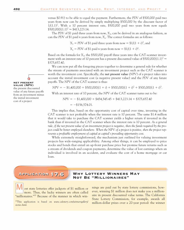
Application 17.6

ost state lotteries offer jackpots of $1 million ormore. Thus, the lucky winners are often called

“millionaires.”10 Because of the manner in which win-

M nings are paid out by state lottery commissions, how-ever, winning $1 million does not make you a million-aire in present discounted value terms. The CaliforniaState Lottery Commission, for example, awards all million-dollar prizes over a 20-year period: the winner


versus $0.91) to be able to equal the payment. Furthermore, the PDV of $500,000 paid twoyears from now can be derived by simply multiplying $500,000 by the discount factor of1/(1.1)2. With a 10 percent interest rate, $500,000 paid two years from now equals$500,000/(1.1)2 � $413,223.14.

The PDV of $1 paid three years from now, X3, can be derived in an analogous fashion, ascan the PDV of $1 paid n years from now, Xn. The correct formulas are as follows:

X3 � PDV of $1 paid three years from now � $1/(1 � i)3, and

Xn � PDV of $1 paid n years from now � $1/(1 � i)n.

Based on the formula for X3, the $500,000 payoff three years into the CAT-scanner invest-ment with an interest rate of 10 percent has a present discounted value of $500,000/(1.1)3 �$375,657.40.

We can now put all the foregoing pieces together to determine a general rule for whetherthe stream of payments associated with an investment project such as the CAT scanner isworth the investment cost. Specifically, the net present value (NPV) of a project takes intoaccount the initial investment cost (a negative present value) and the PDV of any futurepayoffs. The NPV of the CAT scanner is thus:

NPV � � $1,400,000 � $500,000/(1 � i) � $500,000/(1 � i)2 � $500,000/(1 � i)3.

With an interest rate of 10 percent, the NPV of the CAT scanner turns out to be:

This implies that, based on the opportunity cost of capital over time, investing in theCAT scanner is not profitable when the interest rate is 10 percent. The same $1.4 millionthat it would take to purchase the CAT scanner yields a higher return if invested in thebank than if invested in the CAT scanner when the interest rate is 10 percent. As a generalrule, if the net present value of an investment project is negative, then the funds required by the pro-ject could be better employed elsewhere. When the NPV of a project is positive, then the project rep-resents a profitable employment of capital at capital’s prevailing opportunity cost.

While extremely straightforward, the mechanism just outlined for valuing investmentprojects has wide-ranging applicability. Among other things, it can be employed to pricestocks and bonds that entail an up-front purchase price but promise future returns such asa stream of dividends and coupon payments, determine the value of lost earnings when anindividual is involved in an accident, and evaluate the cost of a home mortgage or carloan.

Application 17.6 Why Lottery Winners May Not Be “Millionaires”

� �$156,574.01.

NPV � � $1,400,000 � $454,545.45 � $413,223.14 � $375,657.40

10This application is based on www.calottery.com/winnersgallery/stories.html.

net presentvalue (NPV)the present discountedvalue of any future payoffsfrom an investment minusthe initial investmentcost of a project

• Review Questions and Problems 493

Summary

• The aggregate labor supply curve identifies the totalnumber of hours of work that will be supplied to the econ-omy as a whole at different wage rate levels. It is derivedfrom the income-leisure choices of individual workers.• Since the income and substitution effects operate inopposite directions, the aggregate labor supply curve islikely to be quite inelastic and probably bends backwardabove some wage rate.• A major application of the aggregate labor supplycurve, in connection with the aggregate labor demandcurve, is in analyzing the determination of the generallevel of real wages. The aggregate demand curve is essen-tially the marginal product of labor curve. Its position de-pends on the amount of other inputs available (such ascapital), the level of technology, and the productive char-acteristics of the labor force.• Wage rates can differ among jobs and workers for sev-eral reasons, with no tendency for the rates to becomeequal. Equilibrium wage differences can be due to com-pensating wage differentials, differences in human capitalinvestments, and/or differences in ability.

• Economic rent arises when an input supplier is paidmore than the minimum amount necessary to retain theinput in its present use. Supply and demand analysisshows that part of an input’s price represents rent when-ever the input is in less than perfectly elastic supply.• Borrowing-lending and saving-investment marketsinteract to determine both the interest rate on loanedfunds and the rate of return on invested capital. In equi-librium, the interest rate on loaned funds and the rate ofreturn on invested capital tend to be equal, ignoring anydifferences in risk, tax treatment, and the like. The inter-est rate thus acts to equalize the willingness of people togive up present consumption for future consumption(marginal rates of substitution) and the real net marginalproductivity of investment.• The equilibrium interest rate may be used to deter-mine the net present value of various types of investmentprojects. Profit maximization dictates that projects with apositive net present value should be undertaken.

Review Questions and Problems

Questions and problems marked with an asterisk have solutions given inAnswers to Selected Problems at the back of the book (pages 583–584).

17.1. Edie chooses to work 90 hours per week when the wagerate is $16 per hour. If she is offered time-and-a-half ($24 perhour) for “overtime work” (that is, hours in excess of 90 perweek), will she choose to work longer hours? Support your re-sults with a diagram.

17.2. If workers differ widely in their preferred hours of work ata given wage rate, would you expect to see all firms set the work-week at the average preferred level? Why or why not?

*17.3. Jeeves works 40 hours a week at a $7.50 wage rate. Heunexpectedly inherits a trust fund that pays him $200 per week.

How does inheritance of the trust fund affect his budget line?Will he continue to work 40 hours a week? Will his total in-come rise by $200 a week?

*17.4. Can a person choose to work so much less at a higherwage that her total earnings decline? Show the income and sub-stitution effects implied by that outcome.

17.5. “Kevin (a highly skilled businessman) earns $150,000 ayear. If he were to return to his native New Guinea (where thereare more limited business opportunities), Kevin would be able toearn only $5,000 a year. This proves both that Kevin doesn’t de-serve his high salary and that wages are arbitrarily set in theUnited States.” Evaluate this statement.

is paid $50,000 immediately and $50,000 in each suc-ceeding year for the next 19 years. By paying off on theinstallment plan, the Commission pays a $1-million-winner much less than $1 million in present discounted

value terms. If the prevailing interest rate is 10 percent,for instance, the present discounted value of $1 millionpaid out in equal installments of $50,000 each over 20years is slightly less than $426,000.

17.6. In general, the aggregate demand for and the supply oflabor increases over time. Can we predict what will happen toreal wage rates and employment over time? What factors are re-sponsible for the shift in the demand curve? In the supply curve?

*17.7. “Since only a few people have the ability to become nu-clear physicists, the long-run supply curve of nuclear physicists isvertical.” True or false? Explain.

17.8. Discuss the three reasons for equilibrium wage rate differ-ences given in the text. Which one, or more, accounts for differ-ences in wage rates between engineers and elementary schoolteachers? College professors and high school teachers? Basket-ball superstars and basketball coaches? Doctors and lawyers?

17.9. If workers had identical preferences and were equally ableto perform any job, would all wage rates be equal?

17.10. If Wayne Gretzky’s supply curve of hours of work to pro-fessional hockey is vertical, does this imply that all of his laborearnings represent economic rent?

17.11. What do we mean when we say that capital is produc-tive? How do we measure this productivity? What does produc-tivity have to do with the investment demand curve?

17.12. “In equilibrium, the interest rate equates the willingnessof people to give up present goods in return for future goods andthe ability of the economy to transform present goods into fu-ture goods.” Explain.

17.13. How does the interest rate serve to equalize the desiredrate of saving and the desired rate of investment? Would thisfunction be served if the government placed an upper limit onthe interest rate lenders could charge? How would such a law af-fect the amount of investment undertaken?

*17.14. In Figure 17.12, will the aggregate demand for labor inyear 2 be higher if investment is K1 or K2 in year 1? Why?

17.15. If the union shown in Figure 17.8 wishes to maximizethe total wage payments made to its members, what wage andemployment levels should be selected? Explain your answer.

17.16. In the example of the hospital administrator and theCAT scanner discussed in Section 17.11, is the net presentvalue positive if the interest rate is 5 percent?

17.17. Suppose that you are considering purchasing a corporatebond promising to pay a $1,000 “coupon” in each of the nextfive years. If the interest rate is 10 percent, what will be theprice for such a bond if the bond market is competitive? Willthe bond’s price rise or fall if the interest rate rises to 20 percent?What do your answers imply about the nature of the relation-ship (inverse or direct) between bond prices and the interestrate?

17.18. A speeding car swerves to avoid a rattlesnake slitheringacross a road but accidentally runs over and kills a lawyerwalking along the side of the road. The lawyer was expected to

make $90,000 per year over the next and final 10 workingyears of her life before her untimely demise. If the interest rateis 10 percent and the lawyer’s family sues the driver, for howmuch can the family sue in terms of lost earnings due to theaccident?

17.19. A Fijian island resort offers customers the opportunityto buy 30 vacation days at current prices with the opportunity tospend the purchased days on the island anytime over the next 5years. The money on any days not spent on the island, plus 10percent annual interest, is refundable at the end of the 5 years. Ifthe interest rate over the same period on a typical money marketfund is expected to be only 5 percent, is investing in the vaca-tion days a good idea? Explain your answer.

17.20. Why might a medical doctor who has established a lu-crative practice reduce her patient load and spend more time onthe golf course or tennis court? Explain using a graph of a laborsupply curve.

17.21. In 1999, tobacco companies agreed to settle a lawsuitbrought by attorneys general from 46 states. According to theterms of the settlement, the companies are required to pay $206billion to the states over 25 years in equal annual installments.Explain why the net present value of the settlement to the statesis likely to be far less than $206 billion.

17.22. At any one point in time the supply of lawyers in theUnited States is relatively fixed. Since lawyers are an input tostructuring new companies and business transactions, explainwhy the growth of the Internet economy generated some eco-nomic rents for lawyers. (Note: Whereas law firms historicallyhad taken their cues regarding salaries from established NewYork partnerships, by the late 1990s Silicon Valley firms hadbecome the trend-setters. In 1999, for example, several Sili-con Valley law firms began offering starting salaries of$125,000 to first-year attorneys in contrast to the $91,000 of-fered by established New York partnerships. The New Yorkpartnerships had to play catch-up with their Silicon Valleycounterparts.)

17.23. High-tech industries are not extensively unionized inthe United States. Explain why this is the case, knowing thatsoftware programming, semiconductor manufacturing, and evencustomer service representative positions can be outsourced bycompanies such as Intel, Microsoft, and Amazon to locations inIndia, Singapore, and Malaysia. Rely on the model of input mar-ket monopoly developed in Section 17.6 in your answer.

17.24. On average, television news reporters are better look-ing than newspaper reporters. Explain why this might be thecase, relying on the discussion in Section 17.4 regarding wagedifferences.

17.25. Workers in countries such as Sweden and Germanywork fewer hours per week, on average, than do workers in theUnited States. Does this mean that Swedes and Germans are


• Review Questions and Problems 495

lazier than Americans? Explain how laziness could be inter-preted in the context of the work–leisure choice model devel-oped in this chapter. What other information might you want togather to determine whether Swedes or Germans were indeedless work-oriented than Americans?

17.26. The biotech start-up Genentech has to pay a muchhigher interest rate on any funds it borrows relative to estab-lished pharmaceutical giant Eli Lilly and Company. Why wouldthis be the case if both firms have access to the same capitalmarkets and lending institutions?

chapter 17 · chapter 17 wages, rent, ... application17.3 the returns to investing in a ba and an...

Documents