Chapter 2

Preparing Data Using Structured Query Language (SQL)

[H1] Learning Objectives

[INSERT NL]

1. Use basic standard query language (SQL) commands to manipulate data

2. Select an appropriate set of predictors, including predictors that are rare, obvious, and not

in the causal path from treatment to outcome

3. Identify and clean typical contradictory data in electronic health records

[END NL]

[H1] Key Concepts

[INSERT BL]

Structured query language (SQL)

Primary and foreign keys

SELECT, FROM, CREATE, WHERE, HAVING, GROUP BY, ORDER BY, and other

commands

Inner, outer, left, right, full, and cross joins

GETDATE, CONCAT, STUFF functions

RANK, RAND commandsfunctions

Rare, obvious, causal pathways

Comorbidity versus complications

Landmark, forward, and backward looks

[END NL]

1

[H1] Chapter in a Glance

This chapter introduces standard query language (SQL) and how data can be prepared for

analysis. Data preparation is fundamental to analysis. Without proper preparation of the data, the

analysis can be misleading and erroneous. Details matter—the way each variable in the analysis

is defined affects how predictive it will be. Nothing works better for data preparation than SQL.

Therefore, this chapter spends a great deal of time on the use of SQL. It then shows how SQL

can be used to avoid some common data errors (e.g., dead or unborn patients visiting the clinic).

[H1] SQL Is a Necessary Skill

Data in electronic health records (EHRs) are in multiple tables. Patient information is in one

table. Prescription data are in another. Data on diagnoses are often in an outpatient encounter

table. Hospital data are in still another table. An important first step in any data analysis is to pull

various variables of interest into the same table. Combining data from multiple tables leads to a

large—often sparse—new table, where all the variables are present but many have missing

values. For example, patient X could have a diagnosis and prescription data but no hospital data

if she was never hospitalized. Patient Y could have a diagnosis, prescription, and hospital data

but be missing some other data (e.g., surgical procedure) if he did not have any surgery. The

procedure to pull the data together requires the use of standard query language (SQL).

Before any analysis can be done, data must be merged into a single table, often called the

matrix format, so that all relevant variables are present in the same place. Many statistical books

do not show how this could be done and thus leave the analyst at a disadvantage in handling data

from EHRs. These books do not teach use of SQL. In contrast, I do. I take a different approach

from most statistical books and believe that SQL and data preparation are essential components

of data analysis. An analyst who wants to handle data in EHRs needs to know SQL; there are no

2

ifs, ands, or buts about this. Accurate statistical analysis requires careful data preparation and

data preparation requires SQL. Statisticians who learn statistics without a deep understanding of

data preparation may remain confused about their data, a situation akin to living your life not

knowing your parents, where you came from, or, for that matter, who you are. You can live your

life in a fog, but why do so? Knowing the source of the data and its unique features can give the

analyst insight into anomalies in the data.

Statisticians spend most of their time preparing data—perhaps 80 percent, which is more

than is spent actually conducting the analysis. Ignoring tools for better preparation of data would

significantly handicap the statistician. Knowing SQL helps with the bulk of what statistical

analysts do, which is why training in it is essential and fundamental.

Decisions made in preparing the data could radically change statistical findings. These

decisions need to be made carefully and transparently; the analyst must make every attempt to

communicate the details of these preparations to the manager. Decisions made in preparing the

data should be well thought out—otherwise good data may be ruined with poor preprocessing.

Some common errors in preparing data include the following:

[INSERT NL]

Visits and encounters reported for deceased patients. For example, when a

patient’s date of visit or date of death is entered incorrectly, it may look like dead

patients (zombies) are visiting the provider. Errors in entry of dates of events

would skew results; thus, cleaning up these errors is crucial.

Inconsistent data. Examples might be a pregnant male or negative cost values.

Inconsistent data must be identified and steps must be taken to resolve these

inconsistencies.

3

Incongruous data. After a medication error, one would expect to see long hospital

stays rather than a short visit. If that is not the case, the statistician should review

the details to see why not.

Missing information. Sometimes, missing information could be replaced with the

most likely response; other times, missing information could be used as a

predictor. For example, if a diagnosis is not reported in the medical record, the

most common explanation is that the patient did not suffer from the condition.

Sometimes the reverse could be true. If a dead emergency room patient is missing

a diagnosis of cardiac arrest, it is possible that there was no time to diagnose the

patient but the patient had the diagnosis. For example, Alemi, Rice, and Hankins

(1990) found that missing diagnoses in emergency rooms increases the risk of

subsequent mortality. Before proceeding with the analysis, missing values must

be imputed. One must check to see whether data are missing at random or

associated with outcomes. There are many different strategies for dealing with

missing values, and the rationale for each imputation should be examined.

Double-counted information. When data are duplicated because analysts joined

two tables using variables that have duplicate values, errors commonly occur.

[END NL]

In short, a great deal must be done before any data analysis commences. The analyst

needs a language and software that can assist in preparation of data. Of course, we do not need

statisticians to become computer programmers. Thankfully, SQL programming is relatively easy

(there are few commands) and can be picked up quickly. This chapter exposes the reader to the

most important SQL commands. These include SELECT, GROUP BY, WHERE, JOIN, and

4

some key text manipulation functions. These commands are for the most part sufficient for most

data preparation tasks.

[H1] What Is SQL?

SQL is a language for accessing and manipulating relational databases. SQL was organized by

the American National Standards Institute, meaning that its core commands are the same across

vendors. The current standard is from 1999, which is a long time for a standard to remain stable.

This longevity is in part a result of the fact that SQL is well suited to the task of data

manipulation. The data manipulation portion of SQL is designed to add, change, and remove

data from a database. In this chapter, we primarily focus on data manipulation commands, which

include things such as commands to retrieve data from a database, insert data in a database,

update data already in the database, and delete data from a database.

SQL also includes data definition language. These commands are used to create a

database, modify its structure, and destroy it when you no longer need it. There are also different

types of tables—for example, temporary tables of data that are deleted when you close your SQL

data management software. We will also discuss data definition commands later in this chapter.

Finally, SQL also includes data control language. These commands protect the database

from unauthorized access, from harmful interaction among multiple database users, and from

power failures and equipment malfunctions. We will not cover these commands in this chapter.

[H1] Learn by Searching

Users usually learn the format for an SQL command through searches on the web. I assume that

you can do so on your own. In fact, whenever you run into an error, you should always search for

the error on the web. On the web, you will see many instances of others posting solutions to your

problem. Do this first, because it is the best way to get your problems solved. Most students of

5

SQL admit that they learned more from web searches than any instruction or instructor. The

beauty of such learning is that you learn just enough to solve the problem at hand.

[H1] Common SQL Commands

Different implementations of SQL exist. In this chapter, we use the Microsoft SQL server’s

version. Other versions of SQL, such as dynamic SQL or Microsoft Access, are also available. If

the reader is familiar with the concept of code laid out here, she can also find on the web the

equivalent version of the code in a different language. Learn one and you have almost learned all

SQL languages.

[H2] Primary and Foreign Keys

In EHRs, data reside in multiple tables. One of the fields in the table is a primary key, a unique

number for each row of data in the table. All of the fields in the table provide information about

this primary key. For example, we may have a table about the patient, which would include

gender, race, birthday, and contact information, and a separate table about the encounter. The

primary key in the patient table is a patient identifier, such as medical record number. The

primary key for the encounter table is a visit identification number.

The fields in the patient table (e.g., address) are all about the patient; the fields in the

encounter table (e.g., diagnoses) are all about the encounter. The relationships among the tables

are indicated through repeating the primary key of one table in another table. In these situations,

the key is referred to as a foreign key. For example, in the encounter table, we indicate the patient

by providing the field “patient ID.” To have efficient databases with no duplication, database

designers do not provide any other information about the patient (e.g., his address) in the

encounter table. They provide the address in the patient table, and if the user needs the address of

6

the patient, then she looks up the address using the ID in the patient table. In other words,

databases use as little information as they can to preserve space and to improve data analysis

time. The “FROM” command specifies which tables should be used.

[H2] SELECT and FROM Command

SQL reserves some words to be used as its command. These words cannot be used as name of

fields or as input in other commands. They are generally referred to as reserve words, meaning

these words are reserved to describe commands in SQL. The SELECT command is the most

common reserve word in SQL. It is almost always used. Its purpose is to filter data. It focuses the

analysis on columns of data (i.e., fields) from a table. Here is the general form of the command:

[LIST FORMAT]

SELECT column1, column2, . . .

FROM table_name;

[END LIST]

SELECT is usually followed by one or more field names separated by commas. The FROM

portion of the command specifies the table it should be read from. Here is an example of the

SELECT command:

[LIST FORMAT]

SELECT id

, firstname

FROM #temp

[END LIST]

7

The SELECT command is asking the software to report on a variable or field called “id” and

another field called “firstname.” The convention is to start each field name on a new line

preceded by the comma, so if the analyst wants to delete a field name, she can easily do so by

deleting the entire line. If necessary, the field names can be replaced with *, in which case the

SELECT command will list all fields in the table:

[LIST FORMAT]

SELECT TOP 20 * FROM #temp

[END LIST]

The above command tells the server to return the top 20 rows of data from the temporary file

titled “temp.” The top 20 modification of the SELECT command is used to restrict the display of

large data and enable faster debugging.

The prefix to a table must include the name of the database and whether it is a temporary

or permanent table. To avoid repeatedly including the name of the database in the table names,

the name of the database is defined at the start of the code with the USE command:

[LIST FORMAT]

USE Database1

[END LIST]

The code is instructing the computer to use tables in database 1. Once the USE command has

been specified, then the table paths that specify the database can be dropped.

In addition, the query must identify the type of table that should be used. The place where

a table is written is dictated by its prefix. A prefix of “dbo” indicates that the table should be

8

permanently written to the computer data storage unit, essentially written as a permanent table

inside the database. These tables do not disappear until they are deleted.

[LIST FORMAT]

FROM dbo.data

[END LIST]

This command says that the query is referencing the permanent table named “data.” One can also

reference temporary tables such as

[LIST FORMAT]

FROM #data

[END LIST]

The hash tag preceding the table name says that the query is referencing a temporary table. These

types of tables disappear when the query that has created it is closed. These data are not written

to the computer’s storage unit.

A prefix of double hash tags, ##, indicates that the table is temporary but should be

available to all open windows of SQL code, not just the window for the session that created it.

This is particularly helpful in transferring temporary data to procedures, which are parts of code

that are in a different location. Thus, a single hash tag prefix indicates a temporary local file, a

double hash tag prefix indicates a global temporary file, and the prefix dbo marks a permanent

file.

[H2] Creating Tables and Inserting Values

In this section, we review how CREATE TABLE and INSERT VALUES can be used to create

three tables and link them together using SQL. Assume that you need to prepare a database that

9

contains three entities: patients, providers, and encounters. For each of these three entities, we

need to create separate tables. Each table will describe the attributes of one of the three entities.

Each attribute will be a separate field. Most of the time, there is no need to create a table or insert

its values, as the data needed are imported. Imports often include the table definition and field

names. Sometimes the tables are not imported and must be created using SQL. To create a table,

we need to specify its name and its fields. The command syntax is the following:

[LIST FORMAT]

CREATE TABLE table_name (

column1 datatype,

column2 datatype,

column3 datatype,

. . .

);

[END LIST]

The column parameters specify the names of the fields of the table. The “datatype” parameter

specifies the type of data the column can hold. Data types are discussed on various online sites,

but the most common are variable character, integer, float, date, and text. Always consult the

web for the exact data types allowed in your implementation of SQL code, as there are variations

in different implementations.

The patient attributes include first name, last name, date of birth, address (street name,

street number, city, state, zip code), and e-mail. First name is a string of maximum size 20. Last

name is a string of maximum size 50. These are not reasonable maximum lengths; many names

and last names will exceed these sizes, but we are trying a simple example. Zip code is an integer

10

with no decimals. Date of birth is a date. The state field contains the state the patient lives in. The

patient’s telephone number could be text. A patient ID (autonumber) should be used as the

primary key for the table. When the ID is set to autonumber, the software assigns each record the

last number plus one—each record has a unique ID, and the numbers are sequential and with no

gap.

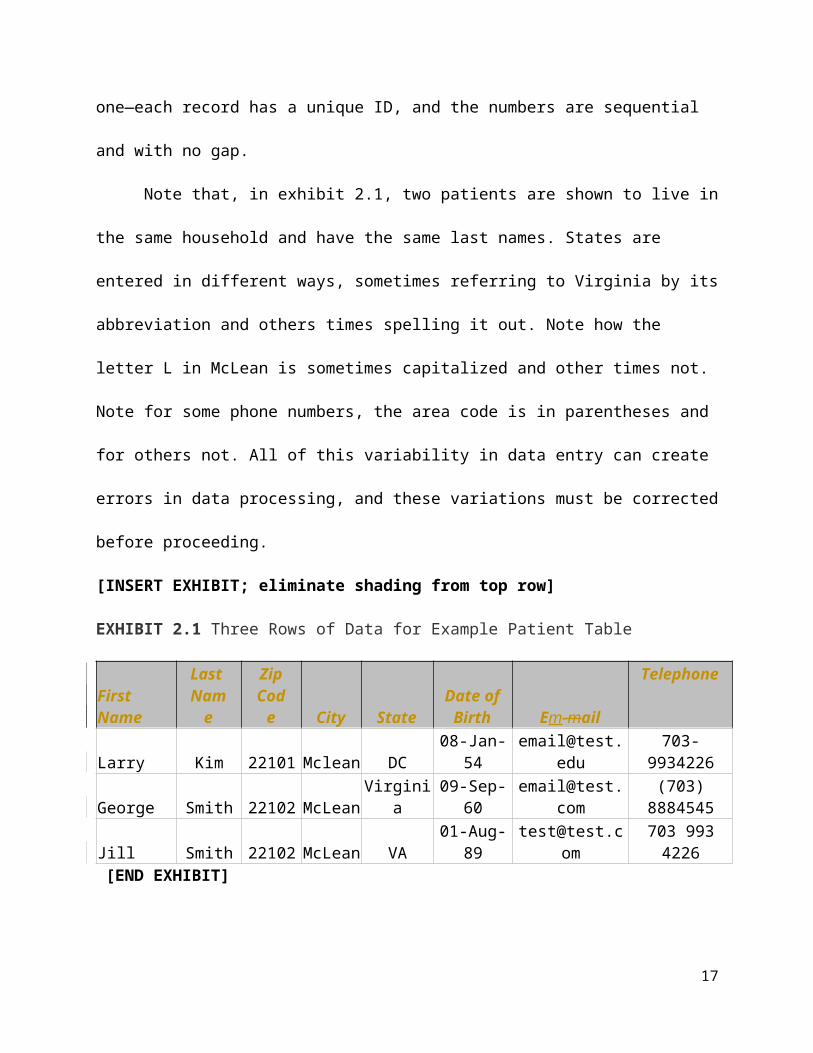
Note that, in exhibit 2.1, two patients are shown to live in the same household and have

the same last names. States are entered in different ways, sometimes referring to Virginia by its

abbreviation and others times spelling it out. Note how the letter L in McLean is sometimes

capitalized and other times not. Note for some phone numbers, the area code is in parentheses

and for others not. All of this variability in data entry can create errors in data processing, and

these variations must be corrected before proceeding.

[INSERT EXHIBIT; eliminate shading from top row]

EXHIBIT 2.1 Three Rows of Data for Example Patient Table

First Name

Last Name

Zip Code City State

Date of Birth Em-mail

Telephone

Larry Kim 22101 Mclean DC 08-Jan-54 email@test.edu 703-9934226George Smith 22102 McLean Virginia 09-Sep-60 email@test.com (703) 8884545Jill Smith 22102 McLean VA 01-Aug-89 test@test.com 703 993 4226 [END EXHIBIT]

Here is a code that can create the patient table. Field names are put in brackets because

they contain spaces. As mentioned earlier, the # before the table name indicates that the table is a

temporary table that will disappear once the SQL window is closed. The patient ID is generated

automatically as an integer that is increased by 1 for each row of data:

[LIST FORMAT]

CREATE TABLE #Patient (

[First Name] char(20),

11

[Last Name] char(50),

[Street Number] Int,

[Street] Text,

[Zip Code] Int,

[Birth Date] Date,

[Email] Text,

[State] Text,

[Phone Number] Text,

[Patient ID] int IDENTITY(1,1) PRIMARY KEY

)

[END LIST]

The provider attributes are assumed to be first name (size 20), last name (size 50),

whether they are board certified (a yes/no value), date of hire, telephone entered as text, and

e-mail entered as no longer than 75 characters. Employee’s ID number should be the primary key

for the table. Exhibit 2.2 shows the first three rows of data for providers; note that one of the

providers, Jill Smith, was previously described in exhibit 2.1 as a patient.

[INSERT EXHIBIT; remove shading from top row]

EXHIBIT 2.2 Three Rows of Data for Example Providers Table

First Name Last Name Board Certified? E-mail Telephone Employee

IDJim Donavan Yes jl@w.com 3456714545 452310Jill Smith No js@w.com 3454561234 454545George John Yes g@w.com 3104561234 456734

[END EXHIBIT]

In SQL servers, there is no “Yes/No” field. The closest data type is a bit type, which

assigns it a value of 1, 0, or null. Also, note again that the provider ID is generated automatically.

12

Here is the code that will create this table:

[LIST FORMAT]

CREATE TABLE #Provider (

[First Name] char(20),

[Last Name] char(50),

[Board Certified] bit,

[Date of Hire] Date,

[Phone] Text,

[Email] char(75),

[Patient ID] int IDENTITY(1,1) PRIMARY KEY

);

[END LIST]

[INSERT EXHIBIT; remove shading from top row]

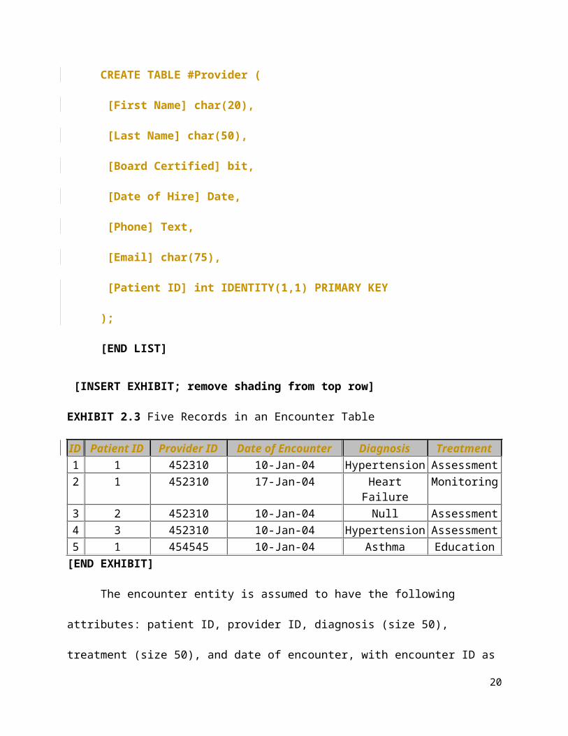
EXHIBIT 2.3 Five Records in an Encounter Table

ID Patient ID Provider ID Date of Encounter Diagnosis Treatment1 1 452310 10-Jan-04 Hypertension Assessment2 1 452310 17-Jan-04 Heart Failure Monitoring3 2 452310 10-Jan-04 Null Assessment4 3 452310 10-Jan-04 Hypertension Assessment5 1 454545 10-Jan-04 Asthma Education

[END EXHIBIT]

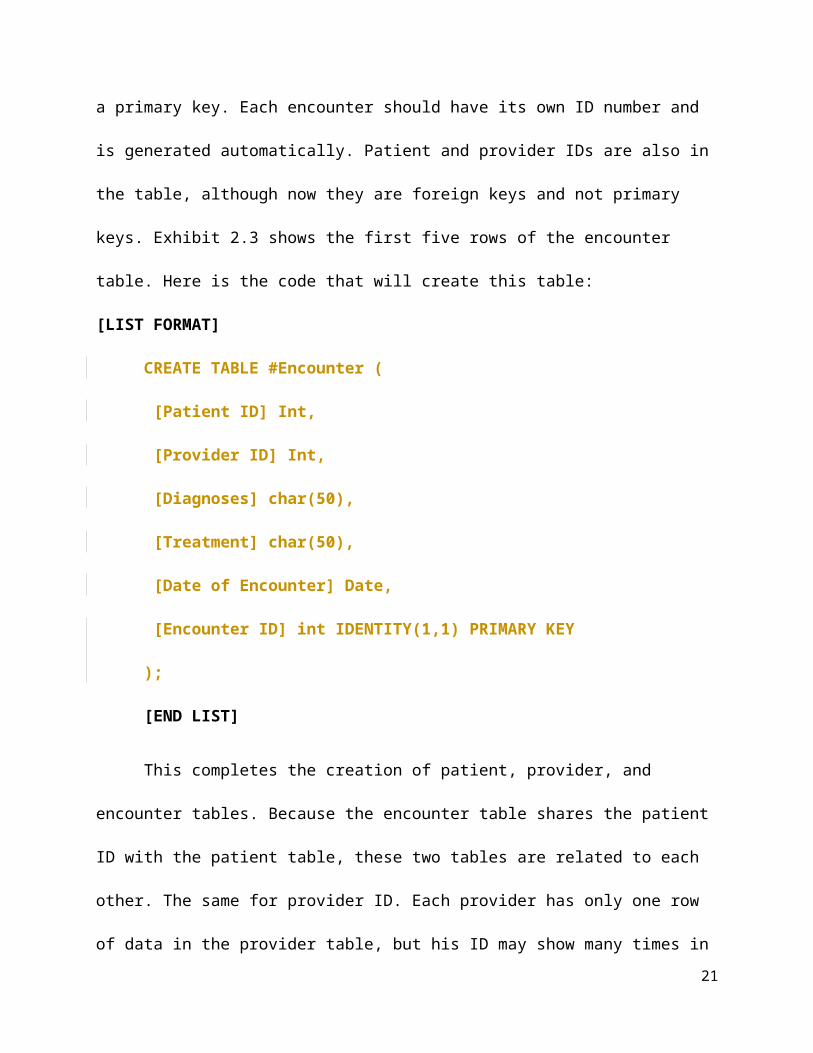
The encounter entity is assumed to have the following attributes: patient ID, provider ID,

diagnosis (size 50), treatment (size 50), and date of encounter, with encounter ID as a primary

key. Each encounter should have its own ID number and is generated automatically. Patient and

provider IDs are also in the table, although now they are foreign keys and not primary keys.

13

Exhibit 2.3 shows the first five rows of the encounter table. Here is the code that will create this

table:

[LIST FORMAT]

CREATE TABLE #Encounter (

[Patient ID] Int,

[Provider ID] Int,

[Diagnoses] char(50),

[Treatment] char(50),

[Date of Encounter] Date,

[Encounter ID] int IDENTITY(1,1) PRIMARY KEY

);

[END LIST]

This completes the creation of patient, provider, and encounter tables. Because the

encounter table shares the patient ID with the patient table, these two tables are related to each

other. The same for provider ID. Each provider has only one row of data in the provider table,

but his ID may show many times in the encounter table. Similarly, a patient shows once in the

patient table and many times in the encounter table. These relationships are called one-to-many

relationships.

The three connected tables constitute a relational database. Exhibit 2.4 shows the

relationship among patient, encounter, and provider entities in our hypothetical electronic

medical record. In the encounter table, we have two foreign keys: patient ID and provider ID.

These foreign keys link the encounter table to the patient and provider tables.

[INSERT EXHIBIT]

14

EXHIBIT 2.4 Example of Relationships Among Three Tables

[END EXHIBIT]

Now that we have created the three tables and their relationships, we can start putting

data into them. The syntax for inserting values into fields is provided on the web and is as

follows:

[LIST FORMAT]

INSERT INTO table_name (column1, column2, column3, . . . )

VALUES (value1, value2, value3, . . .);

[END LIST]

In this code, columns refer to fields in the table. Values refer to data that should be inserted. For

example, to insert the values into the patient table, we would use the following commands:

[LIST FORMAT]

INSERT INTO #Patient ([First Name], [Last Name], [Street

Number],[Street], [Zip Code], [Birth Date], [Email], [State],

[Phone Number])

VALUES

15

('Farrokh', 'Alemi',Null,Null, 22101, '08/01/1954',

'Test2@gmu.edu',Null, '7039934226'),

('George', 'Smith', Null, Null, 22102, '09/09/1960','t@tes.com',

Null,'7038884545'),

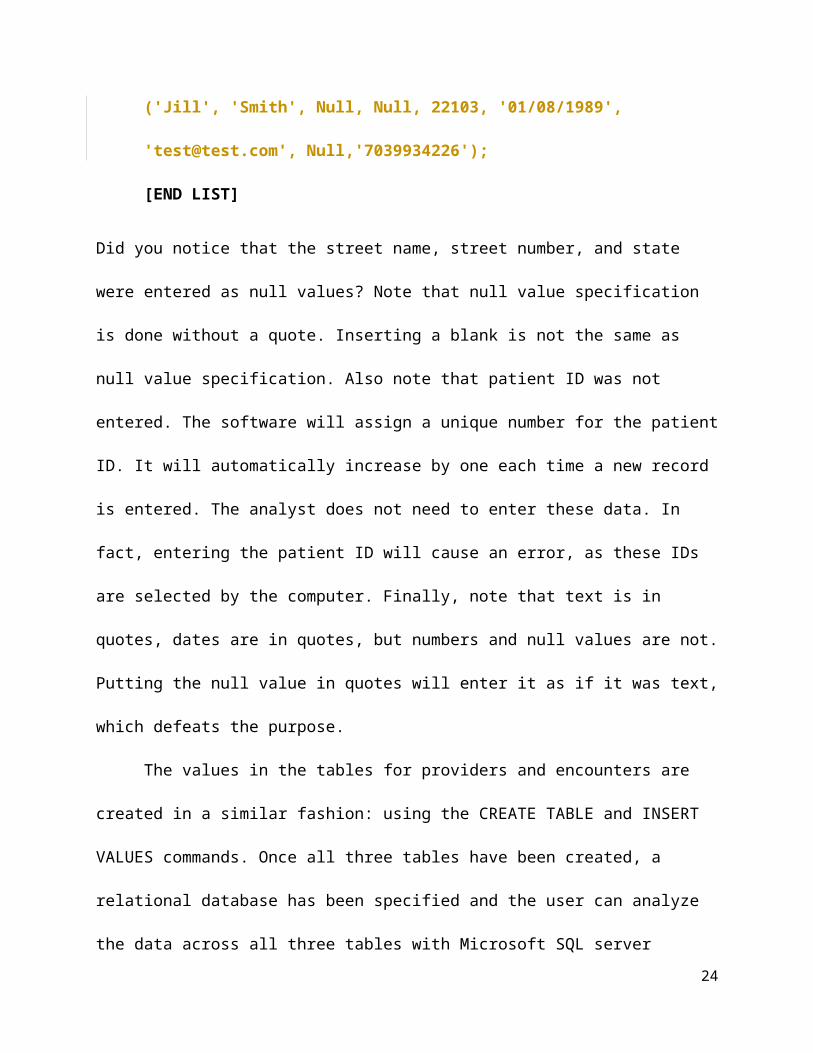
('Jill', 'Smith', Null, Null, 22103, '01/08/1989', 'test@test.com',

Null,'7039934226');

[END LIST]

Did you notice that the street name, street number, and state were entered as null values? Note

that null value specification is done without a quote. Inserting a blank is not the same as null

value specification. Also note that patient ID was not entered. The software will assign a unique

number for the patient ID. It will automatically increase by one each time a new record is

entered. The analyst does not need to enter these data. In fact, entering the patient ID will cause

an error, as these IDs are selected by the computer. Finally, note that text is in quotes, dates are

in quotes, but numbers and null values are not. Putting the null value in quotes will enter it as if it

was text, which defeats the purpose.

The values in the tables for providers and encounters are created in a similar fashion:

using the CREATE TABLE and INSERT VALUES commands. Once all three tables have been

created, a relational database has been specified and the user can analyze the data across all three

tables with Microsoft SQL server Management Studio. Of the three tables, the encounter table

may contain millions of records, while the patient or provider tables are usually smaller.

[H2] Data Aggregation

The GROUP BY command tells the software to summarize the values in a column by subsets of

data. The syntax of the GROUP BY command is as follows:

16

[LIST FORMAT]

SELECT expression1, expression2, . . . expression_n,

aggregate_function (aggregate_expression)

FROM tables

[WHERE conditions]

GROUP BY expression1, expression2, . . . expression_n

[ORDER BY expression [ ASC | DESC ]];

[END LIST]

Any fields, or expressions that contain fields, must either be listed in the GROUP BY command

or encapsulated in an aggregate function in the SELECT portion of the command. Aggregate

functions are identified by reserved words, which database developers write in caps. Aggregate

functions include AVG, where all records in the subset of data are averaged. These functions

include STDEV, where the standard deviations of all records in the subset of data are calculated.

A common aggregate function is COUNT, where all values in the subset are counted. The

COUNTIF counts a value if it meets a condition. COUNT(DISTINCT, Field) calculates distinct

values in the field. Finally, MAX and MIN functions select the maximum or minimum value for

the subset of data. Maximum of a date will select the most recent value, and minimum of a date

selects the first date in our subset.

The WHERE and ORDER BY commands are optional. The WHERE command restricts

the data to the situation where the stated condition has been met. The ORDER BY command lists

the data in a particular ascending or descending order of a set of fields. The following shows an

example.

[LIST FORMAT]

17

USE AgeDx

SELECT top 10 ID, Count(distinct icd9) AS CountDx

FROM dbo.final

WHERE AgeAtDeath is null

GROUP BY ID

ORDER BY Count(distinct icd9) desc;

[END LIST]

The code reports the number of distinct diagnoses for patients who have not died. In

FROM and USE parts, the code specifies that the table named “final” from database AgeDx

should be used. In the SELECT portion of the code, ID is listed but the field “icd9” is

encapsulated in an aggregate function. ID is listed without an aggregation function because it is

already part of the GROUP BY command. Any field that is not part of the GROUP BY

command must be encapsulated into an aggregate function. Make sure you do so in ORDER BY

and SELECT commands. The WHERE command tells the computer to focus on living patients.

Note that variables in the WHERE portion of the code do not need to be encapsulated into an

aggregate function. The WHERE command is executed before the GROUP BY command. In

large data sets, the use of the WHERE command can make GROUP BY computations much

faster. The format of COUNT function leads to reporting the number of distinct diagnoses for

each patient. The resulting data look like this—each ID is followed by the count of their

diagnoses. ID 134,748 has 195 distinct diagnoses:

[INSERT UNNUMBERED EXHIBIT]

ID CountDx

134748 195

18

153091 187

244694 187

728678 184

694089 180

571207 179

222254 178

756012 176

636920 176

541352 175

[END UNNUMBERED EXHIBIT]

The GROUP BY command summarizes the fields for subsets of data. If you summarize

one field in your query, all listed fields must be summarized. The WHERE command is executed

before summarizing the data. If you wish to apply a criterion after summarizing the data, you can

use the HAVING command.

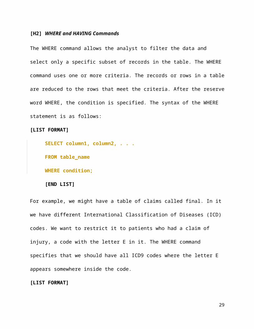
[H2] WHERE and HAVING Commands

The WHERE command allows the analyst to filter the data and select only a specific subset of

records in the table. The WHERE command uses one or more criteria. The records or rows in a

table are reduced to the rows that meet the criteria. After the reserve word WHERE, the

condition is specified. The syntax of the WHERE statement is as follows:

[LIST FORMAT]

SELECT column1, column2, . . .

FROM table_name

WHERE condition;

19

[END LIST]

For example, we might have a table of claims called final. In it we have different International

Classification of Diseases (ICD) codes. We want to restrict it to patients who had a claim of

injury, a code with the letter E in it. The WHERE command specifies that we should have all

ICD9 codes where the letter E appears somewhere inside the code.

[LIST FORMAT]

SELECT [icd9]

FROM [AgeDx].[dbo].[final]

WHERE [icd9] like '%E%'

[END LIST]

Examples of the resulting injury codes include IE878.1, IE849.0, and IE878.1. All codes

without the letter E in it are ignored. If we want all noninjury codes instead, “not like” can be

used:

[LIST FORMAT]

WHERE icd9 not like '%E%'

[END LIST]

The criterion “like 'dia%'” matches any text that starts with “dia-,” such as diabetes,

dialog, diagram, and so on. The % sign indicates that wild card matches occur in the text after

“dia-.” If we want any text that ends with “-ion,” then “like '%ion'” can be used. The % indicates

the wild cards are before “-ion.”

For another example, suppose we want to list all diagnoses that have occurred after the

patient is 65 years old. Then the following code would accomplish the goal:

[LIST FORMAT]

20

SELECT *

FROM [AgeDx].[dbo].[final]

WHERE [AgeAtDx] > 65.0

[END LIST]

In the following code, the computer is instructed to include only records where age at

death is less than age at diagnosis. The data are put into the temporary file called “bad data.”

Presumably errors in data entry have led to some cases showing visits after death.

[LIST FORMAT]

SELECT id

, diagnosis

INTO #BadData

FROM dbo.data

WHERE [Age at death]<[Age at Dx]

[END LIST]

The WHERE command must occur prior to the GROUP BY statement. It is executed before

grouping the data. The command HAVING is the same as WHERE but executed after grouping

is done. In this code, we have dropped the WHERE filter and added a HAVING command:

[LIST FORMAT]

SELECT id

INTO #GoodData

FROM dbo.data

GROUP BY ID

HAVING Min([Age at death])>Max([Age at Dx])

21

[END LIST]

The HAVING command is executed after the GROUP BY statement. In GROUP BY, we are

saying that the data should be grouped by unique persons (i.e., unique IDs). Note that now that

we are examining the data by different persons, we no longer can use the fields “age at death” or

“age at diagnosis” without aggregation. A person has many diagnoses, and we need to clarify for

the code how we want the information to be summarized per person. In this case, we are using

the minimum and maximum aggregation functions. In particular, we are taking the maximum

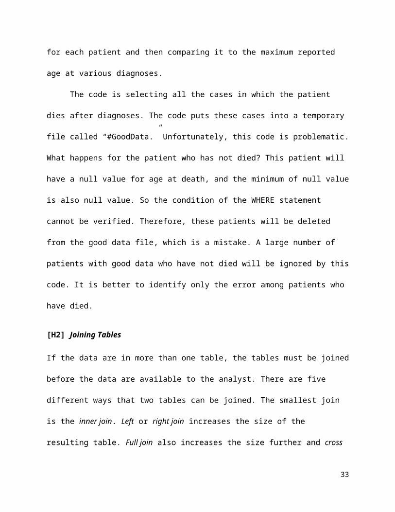
value of age at death for each patient and then comparing it to the maximum reported age at

various diagnoses.

The code is selecting all the cases in which the patient dies after diagnoses. The code puts

these cases into a temporary file called “#GoodData.” Unfortunately, this code is problematic.

What happens for the patient who has not died? This patient will have a null value for age at

death, and the minimum of null value is also null value. So the condition of the WHERE

statement cannot be verified. Therefore, these patients will be deleted from the good data file,

which is a mistake. A large number of patients with good data who have not died will be ignored

by this code. It is better to identify only the error among patients who have died.

[H2] Joining Tables

If the data are in more than one table, the tables must be joined before the data are available to

the analyst. There are five different ways that two tables can be joined. The smallest join is the

inner join. Left or right join increases the size of the resulting table. Full join also increases the

size further and cross join creates the largest resulting table.

[H3] Inner Join

22

This inner join is the most common join in SQL code. The syntax for inner join is given by the

following commands:

[LIST FORMAT]

SELECT column_name(s)

FROM table1 INNER JOIN table2 

ON table1.column_name = table2.column_name;

[END LIST]

Column names in the SELECT portion of the command should be unique across the two

tables or must be prefaced with the table name. The FROM command specifies two or more

tables with the reserved words INNER JOIN in between the table names. This is followed by the

ON statement, which specifies one field from each table. The two fields must be equal before the

content of the tables is joined together.

For example, suppose we have two tables described in exhibit 2.5, one containing

descriptions of diagnosis codes and another reports of encounters that refer to diagnoses. The

description table includes text describing the nature of the diagnosis. The encounter table

includes no text—just IDs and codes that can be used to connect to the description table. A join

can select the text from the “Dx Codes” table and combine it with the data in the encounter table.

An inner join will lead to the listing of all claims in which the diagnostic code has a

corresponding text in the diagnosis table.

[INSERT EXHIBIT]

EXHIBIT 2.5 Encounter and Description Tables

Dx CodesCode ID Code Description1 410.05 Acute MI of anterolateral wall

23

2 250.00 Diabetes mellitus without mention of complication3 250.014 410.05 Acute MI of anterolateral wall5 250.00 Diabetes mellitus without mention of complication7 410.09 Acute myocardial infarction of unspecified sourceNote: The description for code 250.01 is missing, a common problem.

Patient ID

Provider ID

Diagnosis ID

Date

1001 12 1 1/12/2020123 240 5 8/13/2012150 2555 6 9/12/2021

[END EXHIBIT]

A join statement has two parts. The first part names the two tables that should be joined,

and the second part names the fields that should be used to find an exact match. Because table

names are often long, to reduce the need to repeat the name of the table for each field, one can

also introduce aliases in join statements. In this statement, “d” and “e” are aliases for the

[Dx Codes] and [Encounters] tables.

[LIST FORMAT]

SELECT d.*, e.*

FROM [Dx Codes] d inner join [Encounters] e

ON d.[CodeID] = e.[Diagnosis ID]

[END LIST]

Joining the [Dx Codes] and [Encounters] tables will allow us to see a description for each

diagnosis. For example, for patient 1001, we read from the encounters table that the diagnosis ID

is 1. Then from the diagnosis codes table we read that the corresponding description is acute

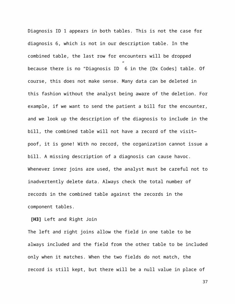
myocardial infarction (MI). Diagnosis ID 1 appears in both tables. This is not the case for

diagnosis 6, which is not in our description table. In the combined table, the last row for

24

encounters will be dropped because there is no “Diagnosis ID” 6 in the [Dx Codes] table. Of

course, this does not make sense. Many data can be deleted in this fashion without the analyst

being aware of the deletion. For example, if we want to send the patient a bill for the encounter,

and we look up the description of the diagnosis to include in the bill, the combined table will not

have a record of the visit—poof, it is gone! With no record, the organization cannot issue a bill.

A missing description of a diagnosis can cause havoc. Whenever inner joins are used, the analyst

must be careful not to inadvertently delete data. Always check the total number of records in the

combined table against the records in the component tables.

[H3] Left and Right Join

The left and right joins allow the field in one table to be always included and the field from the

other table to be included only when it matches. When the two fields do not match, the record is

still kept, but there will be a null value in place of the missing record. Following with the

previous example, here is the command that will combine the two tables using a right join:

[LIST FORMAT]

SELECT d.*, e.*

FROM [Dx Codes] d right join [Encounter] e

ON d.[Code ID] = e.[Diagnosis ID]

[END LIST]

All of the records in the encounters table are included. For diagnosis 1 and 5, the description is

included from the [Dx Codes] table. For the record 6, a null value is included for the description

and for the code. All claims data are still there, but the description of the diagnosis is null when

the description is not available. Note that the diagnosis with code ID 6 is listed, even though the

description is left null because no corresponding diagnosis exists in the description table.

25

In the left join, all records from the [Dx Codes] table are included. Diagnoses that do not

have an encounter are also included, with the missing encounters having null values. The

combined table will list all seven diagnoses. Diagnoses with encounters have the encounters

listed. Diagnoses that do not have encounters list null values (see exhibit 2.6).

[INSERT EXHIBIT; PLEASE RENDER AN EXHIBIT BASED ON WHAT

YOU SEE BELOW. REMOVE SHADING IN UPPER ROWS, AND LEFT-

JUSTIFY CONTENT IN THE STUB COLUMN]

EXHIBIT 2.6 Combined Table After Left Join

[END EXHIBIT]

[H3] Full Join

A full join comprises both left and right joins. Continuing with our example, the code will look

like the following:

[LIST FORMAT]

SELECT d.*, e.*

FROM [Dx Codes] d full join [Encounter] e

ON d.[Code ID] = e.[Diagnosis ID]

[END LIST]

26

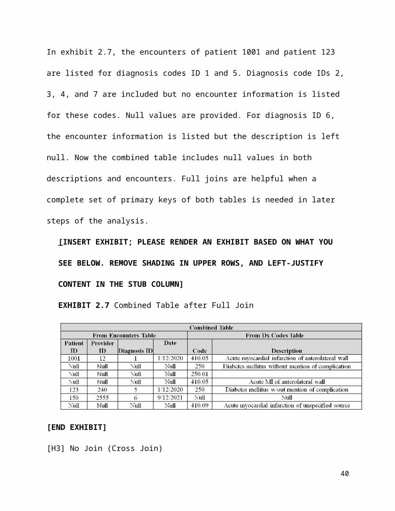
In exhibit 2.7, the encounters of patient 1001 and patient 123 are listed for diagnosis codes ID 1

and 5. Diagnosis code IDs 2, 3, 4, and 7 are included but no encounter information is listed for

these codes. Null values are provided. For diagnosis ID 6, the encounter information is listed but

the description is left null. Now the combined table includes null values in both descriptions and

encounters. Full joins are helpful when a complete set of primary keys of both tables is needed in

later steps of the analysis.

[INSERT EXHIBIT; PLEASE RENDER AN EXHIBIT BASED ON WHAT YOU SEE

BELOW. REMOVE SHADING IN UPPER ROWS, AND LEFT-JUSTIFY CONTENT

IN THE STUB COLUMN]

EXHIBIT 2.7 Combined Table after Full Join

[END EXHIBIT]

[H3] No Join (Cross Join)

In cross join, all records of one table are repeated for each record of the other table. The code

looks like the following (the ON portion of the join is no longer needed):

[LIST FORMAT]

SELECT d.*, e.*

FROM [Dx Codes] d cross join [Encounter] e

ON d.[Code ID] = e.[Diagnosis ID]

27

[END LIST]

A cross join does not specify that any fields should match across the two tables. The

combined table for just the first record of the encounter table will include all six descriptions.

The combined table for the second record of the encounter table will also include all six

descriptions. The combined table for the third encounter will also include six records, each

having a different description. Cross join increases the data size considerably. In our example

of three encounters and six descriptions, cross join created a combined table of 3 × 6, or

18 records. In massive data, you will never see cross joins. Doing so would be

computationally foolish. In smaller data, one might do a cross join but aggressively reduce

some combinations using the WHERE command.

[H2] Text Functions

A number of functions are available in SQL commands that allow users to calculate the value of

the new variable. These functions include arithmetic operations such as add or divide, text

operations such as concatenate, date operations such as days since, and logical operations such

as maximum and if. In this section we focus on text functions.

Many fields in EHRs contain free text that is not classified into coded variables. For

example, medical and nursing notes are typically entered as open text. The names of medications

are typically presented as text fields. If the healthcare organization wants to report the dose of the

medication, users may need to write a code to analyze the name and extract the dose. Analysis

and manipulation of free text is an important part of SQL.

Many functions are available. The CHARINDEX and the PATHINDEX functions return

the location of a substring or a pattern in a string of letters and numbers. LEFT and RIGHT

functions extract a substring, starting from the first or last character of the field. LEN and

28

DATALENGTH functions return the length of the specified string—DATALENGTH in bytes

and LEN in characters. LOWER and UPPER functions change a string to lower or upper case, so

it is easier to read. LTRIM and RTRIM functions remove leading or trailing spaces from a string.

SPACE adds it in. REPLACE switches a sequence of characters in a string with another set of

characters, and SUBSTRING extracts a string from a text field. CONCAT, or the simple use of a

plus sign, attaches two or more strings together. The STUFF function replaces a sequence of

characters with another, starting at a specified position. The exact syntax and meaning of various

SQL functions are available by doing a key word search on the internet. Here we will focus on

syntax for CONCAT and STUFF.

The CONCAT function joins one or more strings, so that the end of one is the beginning

of another. Think of it as a relay run, with each stage of the run being a string. You may also

think of it as a way of adding text to other text. The syntax of the CONCAT function starts with

the reserve word CONCAT:

[LIST FORMAT]

CONCAT(string1, string2, . . . , string_n)

[END LIST]

The parameters of the CONCAT function are specified in parentheses as columns of strings

separated by commas. Alternatively, one could simply write the strings and put a plus sign

between them:

[LIST FORMAT]

string1 + string2 + string_n

[END LIST]

29

Note that all fields must be text, and numbers must be converted to text. At times this may be

confusing. You may see numbers that have a numerical value, but the computer sees them

differently—numbers can be text just as much as letters are. For example, consider a code in

which we want to attach three fields together. Each field is a binary text variable containing 1 or

0. The first field contains “M” for male and “F” for female (see exhibit 2.8). We use the case

function to replace these values with 1 or 0, entered as text. The second field is inability to eat,

which is already in text format, though it shows a number. The third field is inability to sit,

which also contains a text binary field. The plus sign instructs the computer to attach the two

fields.

[INSERT EXHIBIT]

EXHIBIT 2.8 Combining Three Text Fields Using CONCAT

[LIST FORMAT]

, CASE WHEN Gender='M' THEN '1' ELSE '0'

END

+ [Unable to Eat]

+ [Unable to Sit]

AS All

[END LIST]

Gender

Unable to Eat

Unable to Sit All

M 1 1 111M 1 0 110M 0 1 101M 0 0 100F 1 1 011F 1 0 010F 0 1 001

30

F 0 0 000

[END EXHIBIT]

After the code is executed, we have a new column of data titled “All” with three 0 or 1

text entries, each indicating whether the patient is male, whether the patient is unable to eat, and

whether the patient is unable to sit (see the right-hand column in exhibit 2.8). This concatenated

new field contains the information in all three variables and thus may be easier to process. For

example, using GROUP BY All will have the same result as grouping on all three variables

separately. The CONCAT function has joined the values of three fields into one field, each

starting where the other left off.

The STUFF function is also useful for manipulating text in SQL. The STUFF function

first deletes a sequence of characters of a certain length from the field and then inserts another

sequence of characters into the field, beginning at the start of deletion. The deleted length and

inserted string do not need to be of the same length. The syntax of the STUFF function is the

following:

[LIST FORMAT]

STUFF(string1, start, length, add_string)

[END LIST]

There are four parameters in the STUFF function and all four are required and must be

specified before it works. The STUFF function starts with the reserve word “stuff,” and the

function parameters occur inside parentheses. The first entry is the field where we want to make

the change. This field must be a text field. The second entry is an integer or an expression that

produces an integer. The integer indicates where in the string field we would like to make the

change. The third parameter of the function is the length of characters that we want to delete.

31

The last parameter in the STUFF function is a string, which we wish to insert at the start of

location of the deletion. Here is an example:

[LIST FORMAT]

, Stuff('I am happy', 5, 1, ' not ')

[END LIST]

We start with the string “I am happy.” The fifth character is the space between “am” and

“happy.” The code tells the computer to delete 1 character starting with the space. So essentially

we are just deleting the space between “am” and “happy.” In the last parameter, we specify what

should be inserted starting at character 5. Instead of the deleted space, we insert the new string

“not” with leading and trailing spaces. The STUFF function has changed “I am happy” to “I am

not happy.” Here is another example:

[LIST FORMAT]

, Stuff(All, 2, 1, '-')

[END LIST]

In this code, we are instructing the computer to replace the second character in the string variable

All (see exhibit 2.8) with a dash. The All variable was a string variable, containing binary

indications of whether the patient was male, unable to eat, or unable to sit. This code eliminates

the “unable to eat” information from the All variable.

STUFF is a difficult function to work with, as you need to know exactly which character

in the field should be manipulated, as well as the length of the string you must delete. You also

must know the exact text of the strings that should be “stuffed” into the field. But once you know

this information, you can manipulate sentences and words within them. You can cut out one

word and insert another.

32

We should also consider the IIF function. The IIF function is usually thought of as a

logical test of a variable, but it can also be used to check whether certain words are in a text field.

The following is an example of an expression for computing a new field called “Diagnosis”

using the IIF expression:

[LIST FORMAT]

, IIF (ICD9!Description like '%diabetes%', 'Diabetes', 'Other') AS

Diagnosis

[END LIST]

The % sign is a wild card that allows one or more characters to be matched to it. This expression

tells us that if the field “Description” in the table “ICD9” contains the word “diabetes,” the

system will assign to the field “Diagnosis” the value “Diabetes”; in other situations, it will assign

to the field “Diagnosis” the value “Other.”

[H2] Date Functions

In EHRs, all entries are date- and time-stamped. In analysis of data, dates play an important role.

For example, diseases that follow a treatment might be considered complications, and diseases

that precede the treatment might be considered a comorbidity. The same disease at two different

times has different implications for the analysis. Calculating the age of a patient requires finding

the difference between birth date and current date. Calculation of survival rates requires

comparison of date of death and date of cancer treatment. In all of these calculations, we are

examining dates and manipulating them. To facilitate the manipulation of dates, SQL has several

date functions. In this section, we describe several functions used for manipulation of dates and

consider three of the many date functions: GETDATE, DATEPART, and DATEDIFF.

33

One of the most common functions is the GETDATE function. This function produces

the current date. The function has no arguments in the parentheses. If we execute the command

“SELECT GETDATE(),” we get the current date. A date is typically reported in month, day,

year, hour, minutes, seconds, and nanoseconds.

The DATEADD function increases or decreases a starting date by a fixed time interval.

The syntax of the date function will look like this:

[LIST FORMAT]

DATEADD (Interval, Number, Start_Date)

[END LIST]

The interval indicates whether we are adding hours, days, month, quarter, or year. A twice-

repeated h, d, m, q, or y indicates the interval. For example, dd indicates that we want to add

days, and yy indicates that we want to add years. The number indicates how many intervals

should be added. The last parameter gives the starting date and time. The code for adding seven

—a week from today—is the following:

[LIST FORMAT]

SELECT GETDATE() AS [Today]

, DATEADD(dd,7,GETDATE()) AS [This Week]

[END LIST]

From examination of the output of these two lines of code, we can see that the DATEADD

function added seven days to GETDATE for the current date.

The DATAPART function produces a part of the date. It has two parameters. Here is an

example code for obtaining the year part of the current date:

[LIST FORMAT]

34

SELECT DATEPART(yy,GETDATE())

[END LIST]

The first parameter selects which part is needed. If we put in yy, we are indicating that we want

to get the part of the date that is the year. Other parameters are also possible. We could get the

days (dd), the hour (hh), the seconds (ss), the month (mm), the quarter (qq), and so on. The

second parameter indicates the column where the date can be found. In the example code, we are

dissecting the current date into its parts and reporting the year. The output of DATEPART is

always an integer. So, the output for the month of June will be 6 and not the text word “June.”

The DATEDIFF function has three arguments—datepart and two expressions involving

dates. It employs the following syntax:

[LIST FORMAT]

DATEDIFF (datepart, expression1, expression2)

[END LIST]

The datepart indicates the units in which the difference should be expressed. It can be any unit,

from years or all the way down to nanoseconds. Expression 1 and expression 2 are expressions

involving manipulations of columns of dates, times, or combined dates and times. For example,

consider the following calculation of age of a patient born on September 8, 1954. It expresses the

difference between date of birth and current date as age in units of years.

[LIST FORMAT]

SELECT DATEDIFF(yy,'1954-9-8', GETDATE()) AS Age

[END LIST]

If today is June 14, 2018, running this select command results in an estimated age of 64. But this

is not really correct. A common error in date calculations is that they are carried out at the unit

35

specified and all the rest of the information is ignored. Here, we are taking the difference of

current year 2018 and year of birth of 1954 and ignoring that this patient will not be 64 until

September 8, 2018. He is really 63 and 6 months right now, but the SQL is calculating his age as

64 years. Date difference is always calculated at the unit level specified and the rest of the data

are ignored, so one second in the next year will look like one more year, if we are examining the

difference yearly.

Another common problem with date calculations is the format of the column. Many

columns are not in proper date format and must be converted before calculations can be done.

Keep in mind that the entry may look like a date, but the computer may have read it as text.

Consider the following command:

[LIST FORMAT]

SELECT '5/1/2013 9:45:48 AM' AS [Date as Text]

[END LIST]

Though the entry in quotes looks like a date, it is a text field, which we know because it does not

contain any nanoseconds and is in single quotes. This text needs to be converted. But conversion

is not so easy. SQL prevents conversions from text to date, precisely because these conversions

are fraught with data distortions. The entry may be ambiguous. Consider 5/1. Is this May 1 or

January 5? Worse yet, it may contain entries that do not make sense (e.g., a 32-day month). It

may have a misspelled month or even an illogical entry, such as the words “I do not know.”

Before conversion, the analyst must make sure that all values are sensible for conversion from

text to a date.

The CONVERT function converts an expression from one data type to another data type:

[LIST FORMAT]

36

CONVERT(data_type(length), expression, style)

[END LIST]

The command requires the analyst to specify a data type. Numerous data types are allowed,

including date, variable character, integer, or float. Length is an optional command needed

mostly for variable character data types. A variable character data type is a text field with a fixed

length. Expression is the column or manipulation of a column of data that needs to be converted.

Style is optional and there are many different fixed style formats. Styles 100 and 101 are of

particular interest, as these are common formats for dates—a complicated text style. If we want

to convert text to a date, we need to do it in two steps. We first covert the text into variable

characters, here of a length 30 using style 101. This truncates the text field to 30 characters,

something more manageable by the computer. Style 101 also reads the date correctly. Here is

how the code looks like after these two conversions:

[LIST FORMAT]

SELECT CONVERT(datetime,

CONVERT(varchar(30), '5/1/2013 9:45:48 AM', 101)

AS [Date in Date Format]

[END LIST]

The result is a reformatted text as date. Note that nanoseconds are included in the date/time

format that the computer maintains. The computer records all dates with nanoseconds, now set to

zero because it was missing in the text entry. The hard part of working with date functions is the

conversion of string or text input into date formats.

37

[H2] Rank Order Function

RANK and RANK_DENSE functions order the records based on the order of values in one or

more columns. For example, we can find out whether a patient has been repeatedly admitted to

the hospital for the same diagnosis, a situation that happens when the earlier treatment has not

worked and the patient is readmitted for further treatment. RANK differs from the

RANK_DENSE function in how the next rank is assigned when two or more records have the

same rank. If two records have the same rank, RANK function skips the next rank number.

RANK_DENSE does not. For example, if two records are ranked to occur at the same order, at

rank 1, then the rank function will assign rank 1 to both of them and rank 3 to the next record. It

skips rank 2. In contrast, RANK_DENSE will rank the first two at 1 and start the next one at 2.

In exhibit 2.9, we see an example of what is happening to patient 10. He has received

diagnosis 276.1, hyposmolality, repeatedly at different ages. Two of these diagnoses are reported

for the same age. Hence, we see them ranked the same way. We see rank 1, then rank 2; next,

diagnoses are both ranked 3 because they co-occur, now rank 4 is missing and we jump to

rank 5. RANK_DENSE will not have the skip in ranks.

[INSERT EXHIBIT]

EXHIBIT 2.9 Assigned Order Using RANK and RANK_DENSE Functions

ID

Inpatient Diagnosi

s

Age at Diagnosi

s RANKRANK_DENS

E10 I276.1 63.16 1 110 I276.1 64.08 2 210 I276.1 64.25 3 310 I276.1 64.25 3 310 I276.1 64.33 5 410 I276.1 64.66 6 510 I276.1 64.75 7 6

38

[END EXHIBIT]

There is, of course, no difference between rank and rank dense, if no two records have

the same order. This can be guaranteed by grouping the field used to set the order of the records,

a first step that often should be done before using rank functions. When no two records have the

same order, no two have the same rank.

For example, patients may have the same diagnosis on the same date of hospital

admission. Once they are seen by one doctor, and at a different point by another clinician.

Ranking these diagnoses as two different times with the same diagnosis is a mistake. In this

situation, it makes sense to delete the repetitions of the diagnosis for the same person at the same

time. This helps make the ranking task more efficient and more sensible. Here is the syntax for

the rank function:

[LIST FORMAT]

RANK ( ) OVER ([ <partition_by_clause> ] <order_by_clause>)

[END LIST]

The syntax requires specification of the OVER clause, which requires us to specify what field or

fields should be used to order the ranks. The PARTITION clause is optional and describes

whether the rank order should restart in subgroups of the records. Here is an example of the

RANK command:

[LIST FORMAT]

DROP TABLE #Temp

USE AgeDx

SELECT ID, icd9, AgeAtDx

39

, RANK() OVER (PARTITION BY id, icd9 ORDER BY icd9, AgeAtDx)

AS [Repeated Dx]

INTO #Temp

FROM dbo.final

WHERE ID=10

GROUP BY ID, icd9, AgeAtDx

Select * FROM #Temp ORDER BY ID, icd9, [Repeated Dx]

[END LIST]

For computational ease, we can use the WHERE command to filter the data for only the

person with an ID of 10. The GROUP BY command removes duplicates, so RANK and

RANK_DENSE produce the same results. The GROUP BY command will delete any record for

the same patient having more than one instance of the same diagnosis at the same age.

Otherwise, these steps will take a long time to carry out. The RANK command has two clauses

specified. The ORDER BY portion of the command says that we want to set the order based on

diagnosis and age at which it occurs. The PARTITION BY portion of the command says that we

want to organize the ranks to start from 1 for each individual and each diagnosis of the patient.

Exhibit 2.10 provides a portion of the results. In the first row, at 64.66 years, the patient

was hospitalized with diagnosis 041.89, which is an unspecified bacterial infection. This

infection did not repeat, so the rank does not exceed 1. The next disease is 112.0, which is

candidiasis of the mouth. This disease also does not repeat either. The situation is different for

hospitalization with diagnosis 253.6, which is “Other disorders of neurohypophysis.” The patient

was hospitalized for this disease three times, first at the age of 64.25, then at 64.75, and later at

40

65.25. We see that this disease is ranked 1, 2, and 3 for repetition. Repetition also occurs for

disease 272.4, “Unspecified hyperlipidemia.”

[INSERT EXHIBIT]

EXHIBIT 2.10 Output for Rank of Diagnoses for Person with ID 10

ID icd9 AgeAtDx Repeated Dx10 I041.89 64.66 110 I112.0 64.25 110 I253.6 64.25 110 I253.6 64.75 210 I253.6 65.25 310 I263.9 64.91 110 I272.4 64.25 110 I272.4 65.25 210 I275.2 64.91 110 I275.2 65.58 2

[END EXHIBIT]

[H1] Cleaning Data

[H2] Dead Man Visiting

Before the data are merged from different files, it is important to exclude records of patients that

are impossible. For example, sometimes a patient is reported to have visited a clinician after

death. Clearly this is not possible. In rare situations some visits occur after death—for instance,

the transport of a dead patient from home to hospital, autopsy, or postmortality services to family

members. The most common reason for reported encounters with the healthcare system after

death is the incorrect entry of date of death by a clinician or clerk. Such errors rarely occur if the

organization uses the Centers for Medicaid & Medicare Services (CMS) Death Master List; in

recent years, however, CMS has decided against sharing this master list because of identity theft.

Therefore, organizations have to enter the date of death in their medical records by hand, and we

may be left with an erroneous date of death. One of the first steps in cleaning the data is to

41

identify patients whose date of death occurs before the date of various outpatient or inpatient

encounters. The code for identifying such discrepancies may look as follows:

[LIST FORMAT]

DROP TABLE #nonZ

SELECT ID

INTO #nonZ

FROM dbo.data

GROUP BY ID

HAVING (Min(AgeAtDeath)>=Max(AgeAtDx) OR

Min(AgeAtDeath) is null )

[END LIST]

In this code, the SELECT ID command tells the system that we are interested in finding the ID

of the patients. Note that, because this query has only one table, we do not need to identify the

source of the ID field. If two tables were joined, it would be necessary to specify the source of

the data so there is no room for confusion. Thus, we should have used “SELECT dbo.data.ID.”

The INTO command says that we should include these IDs in a file called #nonZ. The “FROM

dbo.data” command says that we want to get this information from a permanent table called data,

which includes both “Age at death” and “Age at diagnosis” fields. The HAVING command says

that two conditions will be used to include patients in our new file. Either the minimum age at

death must be less than the maximum age at diagnosis, or the minimum age at death must be

null. It is important to include the patients with no age-at-death entry because we want to include

patients who have not died. GROUP BY ID says that we want to see only one value for each ID,

no matter how many times the person’s diagnosis occurs at a later time than his death.

42

One alternative is to use the WHERE command instead of the HAVING command. Then

the code will look like this:

[LIST FORMAT]

DROP TABLE #nonZ

SELECT ID

INTO #nonZ

FROM dbo.data

WHERE AgeAtDeath >= AgeAtDx

or ageatdx>0

GROUP BY ID

[END LIST]

This approach is not reasonable. We would delete the erroneous dates but not eliminate the entire

record of the patient. Given that problems with date of death and date of birth affect age at the

time of all visits, the entire record should be eliminated.

[H2] Visits Before Birth

If birthdates are wrong, patients may show visits prior to birth. In these situations, it is important

to identify the person and exclude the entire record of the person. We can add the condition that

age at diagnosis needs to be a positive number at the end of the previous code.

[LIST FORMAT]

DROP TABLE #nonZ

SELECT Id

INTO #nonZ

43

FROM dbo.data

GROUP BY ID

HAVING (Min(AgeAtDeath)>=Max(AgeAtDx) OR

Min(AgeAtDeath) is null)

AND Min(AgeAtDx)>0

[END LIST]

This code says that we should select the ID of the person, one per person. We will drop the

patients who have one or more diagnoses prior to birth. We identify the patients by having a

diagnosis of 0 or a negative age. Once we have the ID of patients whom we want to include in

the analysis, we need to merge these data with the dbo.data to select all the remaining fields.

[H2] Patients with No Visits

In many studies, we are looking for a patient’s encounters with the healthcare system. Sometimes

the entries in a medical record are not for real people, as when a test case was entered. These

patients are typically identified with primary keys that start with ZZZ. Such records must be

excluded before proceeding.

For some patients, there are no encounters with the healthcare system during the study

period. This absence creates doubt about whether these patients are real or simply healthy. If the

period is long—say, a decade—then at least some encounters are expected. In the absence of any

encounter, it is important to explore why this may be occurring. For example, the patient may be

using the facilities to pick up his medications but not for receiving medical services. Other

explanations are also possible. It is important to count how many patients have no encounters

and find out what are the most likely explanations.

44

[H2] Imputing Missing Values

Missing values are another common error. Keep in mind that the medical record is the report of

an encounter. Patients may have encounters that are not reported, as when the patient meets the

clinician in a social gathering. A question arises regarding what should be done with information

not reported in the EHR. The answer depends on what the information is. For example, let us

think through what should be done when the patient has no report of having diabetes. One

possibility is that the patient was not diagnosed with diabetes, in which case we can assume that

the patient does not have diabetes. In this case, we will set the value of the field diagnosis to 0:

[LIST FORMAT]

IIF(Diabetes1 is null, 0, Diabetes1) AS Diabetes2

[END LIST]

This command says that if the field Diabetes1 is null, replace it with 0 and otherwise assign it the

value in Diabetes1 and rename the new field Diabetes2.

One general strategy for imputing missing values is to assume that missing values are the

most common value. Thus, if the diagnosis of diabetes is missing, and most patients in our study

do not have a diabetes diagnosis, then the best approach may be to assume that the patient does

not have it. In the emergency room, however, a missing diagnosis may indicate insufficient time

to establish it. In one study of an emergency room, for example, Alemi, Rice, and Hankins

(1990) found that missing values of myocardial infarction (heart attack) diagnosis were highly

correlated with mortality. In this situation, it is not right to assume that missing diagnoses

indicate normal condition.

45

Treatment is usually reported when given. It may be safe to assume that if a treatment is

not reported, it was not given. Again, it may be important to know whether patient conditions

precluded giving the treatment.

Sometimes when a value is missing, the best approach is to measure it from its nearest

values. For example, if blood pressure is missing in the second quarter of the fiscal year, it may

make sense for the statistician to estimate it from the third quarter. Other times we can impute

the missing value from other available data. Thus, we can impute that the patient is diabetic if

she is taking diabetic medication or if hemoglobin A1c levels (a marker for diabetes) indicate

diabetes. Exceptions occur, especially if medications are used to impute diagnosis. Some

prediabetic patients take Metformin, a drug also used for diabetes, so indicating that those

patients had true diabetes would be erroneous. Physicians may prescribe a medication for a

reason different from the typical use, so if the analyst sees the medicine in the database, he may

think it indicates a diagnosis when it does not. In these situations, he would need to understand

whether the rest of the patient’s record supports the imputation.

[H2] Out-of-Range Data

One way to have more confidence in data in medical records is to find out whether the data are

out of the expected range. A patient whose age is more than 105 years or fewer than 18 may not

be reasonable for our study. In the following code snippet, we use the BETWEEN function to

check for the range of the age:

[LIST FORMAT]

DROP TABLE #InRange

SELECT ID, VisitId

INTO #InRange

46

FROM dbo.data

WHERE AgeAtDx between 18 and 105

and AgeAtDx is not null

[END LIST]

Out-of-range analysis should be done on all variables, not just dates. Note that in this code, the

entire record is not excluded. Only the specific visit with out-of-range age is excluded. Even

though we do not show it here, the visit and patient IDs should be used to merge the calculated

temporary file with the original data, so that all relevant fields, not just IDs, are available for

analysis.

[H2] Contradictory Data

Inconsistencies tell us a great deal about our data. Seemingly impossible combinations may

occur. It is important to examine whether these occurrences are at random and whether there are

any justifications for it. For example, consider a pregnant male. This record is not reasonable.

The following is a code intended to select all data except male subjects who are pregnant:

[LIST FORMAT]

SELECT Id

FROM dbo.data

WHERE Not (Gender = 'Male' and Pregnant = 'Yes');

[END LIST]

Of course, inconsistent data do not arise only with impossible combinations. Some level

of inconsistency may arise among variables that often co-occur. Very tall people may be unlikely

to be in our sample even if their height is possible. If we see a body weight of more than

400 pounds, we wonder if the patient’s weight was taken while he was on a motorized chair.

47

Even among probable events, inconsistent data should raise concerns about quality. When all

fields point to the same conclusion, there is little concern. When some fields suggest the absence

of an event and other fields suggest that the event has occurred, the analyst’s concern is raised,

often requiring human chart reviews or a conversation with the patient. Consider an illustrative

example.

The Agency for Healthcare Research and Quality (AHRQ) has come up with several

measures of quality of care using EHRs. One such measure is the frequency with which

medication errors occur. When a medication error occurs, clinicians are required to indicate it in

the record. However, sometimes this is not done. Sometimes, an activity is done but not recorded

in the right place. Thus, the AHRQ’s patient safety indicator may rely on the frequency with

which heart failure patients are discharged with beta blocker prescriptions (an evidence-based

treatment). However, what if the doctor put the prescription in the note, but the patient filled the

prescription while on a trip to a child’s home in a different state? Such pharmacies would not be

monitored in the healthcare organization’s medication reconciliation files, and in such situations

the analyst would undercount the number of beta blockers. The variation in reporting is one

reason AHRQ recommends that expensive chart reviews be done to verify under- or over-

reporting of patient safety issues. Some chart reviews, however, are not needed if other

indicators are consistent with the reported event.

To see if variables in the EHR are consistent with the reported event, we predict the event

from other variables. Next, comparison of predicted and observed values indicates the extent to

which data are consistent. For example, one would expect that patients who are older, who have

long hospital stays, who have multiple medications, and who have cognitive impairments are

more likely to fall. We can compare the predicted probability of fall to an actual observed fall. If

48

there is negligible probability of fall and the patient has fallen, then something is not right. If

there is high probability of fall and we see consequences of a fall (prolonged hospitalization),

perhaps the patient has fallen and the EHR is not correct. Exhibit 2.11 shows hypothetical

results. Chart reviews may need to be done when low-probability events are reported or high-

probability events are not reported.

[INSERT EXHIBIT]

EXHIBIT 2.11 Reports Inconsistent with Probability of the Event

 

Probability of Fall

Low Mediu

m HighFall reported Not consistent   ConsistentFall not reported Consistent   Not consistent

[END EXHIBIT]

A similar test of consistency can be applied to patient-reported outcomes such as pain

levels (see exhibit 2.12). Obviously, pain is a subjective symptom. Some patients have more

tolerance for pain than others. Some patients treat pain with medications, while others with the

same level of pain refuse medication. One can predict the expected pain level from the patient’s

medical history, the contrast expected, and reported levels.

When patient-reported pain levels do not fit the patient’s medical history, additional steps

can be taken to understand why. For example, the patient’s medical history can be used to predict

the potential for medication abuse. If the patient is at risk and is reporting inconsistent pain

levels, then the clinician can be alerted to the problem and explore the underlying reasons.

[INSERT EXHIBIT]

Exhibit 2.12 Expected and Patient Reported Pain Levels

 

Expected Pain Level

Low Mediu

m High

49

Patient Reported Levels

Low ConsistentNot

ConsistentMediu

mHigh Not Consistent Consistent

[END EXHIBIT]

[H2] Inconsistent Format

In many situations, data are copied into (read into) the database from an external source with the

wrong formatting. In a database, the format of the data must be set before reading the data. There

are many different types, including integer, text, float, date, and real. The CAST and CONVERT

commands allow the user to reassign the type of data. For example, if the field Age is read as

text instead of a numerical value, then the following command will cast it as a numerical float

(a number with a decimal):

[LIST FORMAT]

, CAST (Age as Float) AS Age

[END LIST]

For example, ages 45.5 and 47.9, which may have been previously read as text, are now a

number with a decimal. In converting a field from text to number, a problem arises with text

entries such as the word “Null.” This is not recognized as a null value but as a piece of text with

four letters. A simple CAST will not know what to do in these situations. Instead one should use

a code something like the following:

[LIST FORMAT]

, IIF(Age=’Null’, Null, CAST(Age as Float)) AS Age

[END LIST]

50

The command says that if (shown as IIF) the field Age has a text field with the text “Null,” then

the new field should treat this value as a true null value. Otherwise, it should cast the Age field

as a float.

[H1] Should Data Be Ignored?

[H2] Keep Rare Predictors

Discarding predictors that rarely occur is a common practice in statistics. The logic is that these

rare predictors occur too infrequently to make a difference for an average patient. In EHRs, we

have thousands of rare predictors. Ignoring one has a negligible effect, but ignoring thousands of

rare predictors will have a large impact on the accuracy of predictions for the average patient.

Furthermore, ignoring these predictors will reduce accuracy in the subset of patients who

experience rare diseases. Therefore, I do not recommend the exclusion of rare predictors. This

policy yields a statistical model with thousands of variables, most of which occur in rare

situations. The model will be accurate, but difficult to manage.

[H2] Keep Obvious Predictors

A related issue is whether we should keep obvious predictors. For example, as we predict

diabetes, a patient with diabetic neuropathy is clearly diabetic. There is no need to predict

whether the patient has undiagnosed diabetes or will have diabetes in the future; clearly, he is

diabetic. Some investigators argue that nothing is gained by using a model that makes accurate

predictions in obvious situations. I disagree. These obvious cases should be kept in the model for

two reasons: (1) errors in these cases will lead to clinicians ridiculing the model and abandoning

its use; and (2) in EHRs, crucial information may be missing and obvious predictors can adjust

for missing values. In our example, it may be that a patient is hospitalized with diabetic

51

neuropathy, but for this patient no diabetes was recorded. Diabetes is usually observed in an

outpatient setting. It is possible that the doctor who sees this patient does not use the same EHR

software, and therefore the outpatient mention of diabetes is missing. Keeping obvious predictors

helps the system address missing information.

[H2] Drop Diagnoses That Occur After the Outcome?

Statisticians are concerned with outcome prediction by use of a variable has not occurred until

after an outcome. On the surface, such predictions look tautological—they consist of useless

repetition. For example, if we want to predict whether the patient will develop diabetes,

observing that they suffer from the complications or consequences of diabetes is tautological.

Such predictors should not be part of the analysis. At the same time, we often want to detect

whether a patient has already developed an illness. In these situations, we detect the illness by its

consequences. Therefore, if the purpose is detection, the analyst should include consequences of

the disease.

For example, undiagnosed diabetes, or diabetes not previously reported in the EHR, can

be detected by seeing whether the patient has complications of diabetes, such as renal illness.

Detection and prediction use different sets of predictors. In predictive models, we are looking

forward to establish the risk of future events. In these models, only predictors that occur before

the outcome can be used. In detection, we are looking backward to see if a diagnosis was missed,

and in these models, diagnoses before and after the outcome of interest can be used.

When evaluating predictive models, the practice is to divide the data into two sets:

training and validation. The parameters of the predictive model are estimated in the training-data

set, but the model is tested in the validation set. In the training set, all diagnoses are included as

predictors of the outcome. This means that diagnoses that occur after the outcome or before the

52

outcome are included in estimating the association between the predictor and the outcome.

Validation is different. Here we want to rely only on predictors that occur prior to the outcome.

Therefore, it is important to exclude any diagnosis that occurs after the outcome. This

information is available in the EHR, but not in real life. In real life, we are making a prediction

about the likelihood of the outcome before the outcome has occurred. Therefore, we do not have

access to any diagnosis or other information that arises after the outcome.

[H2] Drop Complications?

Sometimes the available data are reasonable but should be ignored in the context of the analysis

planned. If we are studying the impact of treatment on survival, statisticians should drop

complications from multivariate models. Complications are on the causal path from treatment to

survival. Including them will distort the relationship between treatment and survival. In EHRs,

complications are diagnoses that occur after treatment. Before treatment, the same diagnosis is

considered medical history, and at the time of treatment it is considered comorbidity. This

requires us to drop some of the diagnoses and retain others according to whether they occur

before or after treatment.

In exhibit 2.13, because the patient had an infection and was overweight, a large dose of

antibiotics was given, which distorted the microbes in the patient’s gut. The patient developed

diabetes. If we keep diabetes in our multivariate models, the effect of antibiotics on survival will

be distorted. In these situations, we want to keep comorbidities (i.e., overweight and infection)

but not the treatment complication, which is diabetes.

[INSERT EXHIBIT; render in gray scale, and make ovals transparent (no shading), but

retain “highlighting” around arrows and “Diabetes” oval]

53

EXHIBIT 2.13 Diabetes as a Complication of Treatment

[END EXHIBIT]

Keeping comorbidities but not treatment complications requires a code that drops

diagnoses that occur after treatment. In this code, we remove complications of treatment and

retain all diagnoses that occur prior to, or at the time of, the treatment. In this code, the WHERE

command states that the age of diagnosis should be less than or equal to age at start of treatment.

[LIST FORMAT]

SELECT ID, Diagnosis

FROM dbo.data

WHERE AgeAtDX <= AgeAtTreatment

GROUP BY ID, Diagnosis

[END LIST]

[H1] Time Confusion: Landmark, Forward, and Backward Looks

Data in EHRs are time-stamped. These dates and hours provide a chronology of events that have

occurred in encounters with the healthcare system. Naturally, events for different patients occur

at different times. For the purpose of analysis, we need to start time at a landmark and count

54

progression in time from this landmark. This is called landmark time to distinguish it from

chronological time.

For example, suppose we want to evaluate the impact of a treatment on patients’

outcomes. For some patients, the treatment occurs in January, and for others a month, a year, or a

decade later. Once the treatment occurs, no matter the timing, the outcome must be evaluated in

a predetermined follow-up period after treatment. During this period, the outcome of interest

may or may not occur. To calculate the impact of a treatment on outcome, we would need to set

the chronological time of treatment to zero at the date and time of the patient’s treatment. In all

calculations, the analysis uses time from the landmark event and not the chronological time.

Data from EHRS, which track a patient from birth to death, can be used in different ways

to design a study.. One approach is a retrospective case/control design, in which patients with

and without an intervention are contrasted. In this approach, the statistician defines the cases

(exposed to disease) and controls (not exposed to disease) and looks backward to see whether

patients were exposed to risk factors. Another approach is a cohort design, in which a group of

patients are followed over time. In such a study, the user selects a group of patients and looks

forward in time to see if they have developed a specific outcome or disease. Looking forward for

data is typically done prospectively. In an EHR, where you can see the same patient over time,

you can look forward using existing data.

Exhibit 2.14 is a visual depiction of a cohort design. The outcomes are also observed in

the past but after the organization of the cohort. Because both exposure and examination of

outcomes occur in the past, it is often difficult to distinguish these study designs in EHR data.

The easiest way to tell a case/control study design from a cohort design is to check whether the

study looks forward or backward.

55

[INSERT EXHIBIT; convert to gray scale; make ovals transparent (no shading)]

EXHIBIT 2.14 Historical Cohort and Case/Control Studies

[END EXHIBIT]

[H2] Example of Forward Look for Readmissions

An example may demonstrate the issues that arise in defining either the cohort or the study

design. Suppose we want to study 30-day readmissions among heart failure patients in a hospice

program. To begin with, let us assume that we want to do a cohort study, meaning that we define

a group of heart failure patients in hospice and see how many of them have readmission within

30 days. In this situation, the exposure is to “hospice” and the outcome of interest is 30-day

readmission. Hospice can affect readmissions in different ways. One scenario is that hospice use

reduces active treatment—therefore, patients are less likely to be readmitted and will pass away

without hospitalization. Another scenario is that hospice use may increase treatment, in part

because hospice programs may fail to manage patients’ dyspnea (shortness of breath). Families

troubled by breathing problems of their loved one may choose to return to active treatment. What

56

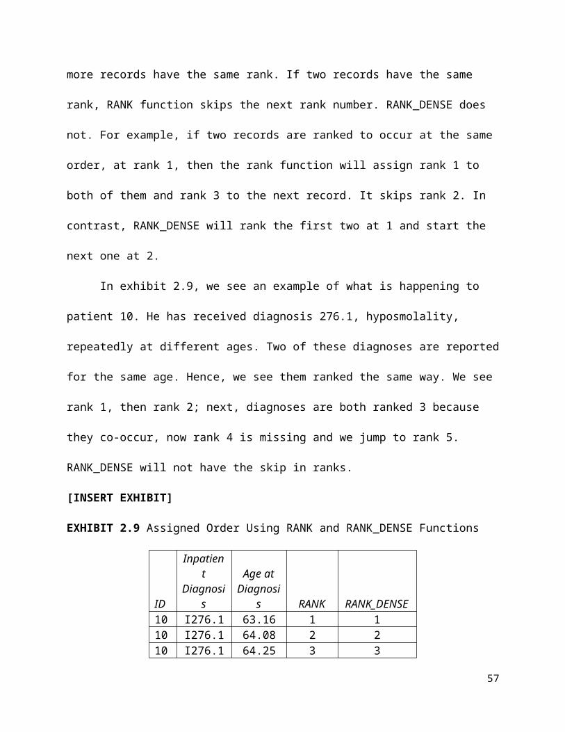
we know from the medical literature is that many heart failure patients die within a few days of

hospice admission; if the patient dies in a hospital that would count as a hospital readmission

within 30 days.

To settle whether hospice use increases or decreases readmissions, the statistician must

look at data. If she wants to use the cohort study design, the first step is to define the exposed and

unexposed cohorts.

One has to define two groups of patients, each constituting a different cohort

(see exhibit 2.15). The first group is the exposed group. These are heart failure patients who use

hospice care; we refer to these as patients as discharged to hospice, even if the patient is

admitted to hospice after a short stay at home. To sharpen the contrast between the exposed and

unexposed groups, we would need to exclude all patients who do not have a primary diagnosis of

heart failure hospitalization.

[INSERT EXHIBIT; render in gray scale; make ovals transparent (no shading)]

EXHIBIT 2.15 Cohort Study of Impact of Hospice on Readmissions

[END EXHIBIT]

The definition of the cohort requires the presence of both the index hospitalization for

heart failure and hospice use; this is because calculation of 30-day readmission requires an index

hospitalization, and exposure requires use of hospice. Therefore, the most reasonable definition

of the cohort is that both conditions must be present. The exposed cohort is compared to the

57

nonexposed cohort, which must have an index hospitalization but no hospice use. Note that

patients who do not have heart failure are excluded from both the exposed and unexposed group.

This is done to sharpen the contrast between the two groups.

Exhibit 2.16 provides some scenarios regarding the overlap between index heart failure

hospitalization and hospice use. Depending on how we define our cohort, some readmissions

will be ignored, and therefore study findings will change. Patient A should not be part of the

cohort because the index hospitalization occurs a long time before hospice use and therefore

these two events are not co-occurring. In contrast, patient B has an index hospitalization near

start of hospice and therefore this patient is considered part of the cohort. Patient C and patient D

are part of the cohort because index hospitalization and hospice use co-occur. Patient E is not

part of the cohort because index hospitalization occurs after hospice use. Patients A, E, and F are

part of the unexposed cohort. Patient A and patient B are both part of the unexposed group, even

though they show that at some point they had hospice use. For these two types of patients,

hospice use and index hospitalization does not co-occur and therefore the conditions for the

landmark event that defines the exposed cohort are not met.

[INSERT EXHIBIT; render in gray scale. Make yellow boxes light gray, blue items

medium gray, and green boxes black]

58

EXHIBIT 2.16 Ways an Index Hospitalization and Hospice May Co-Occur

Note: I = index hospitalization; R = readmission; yellow bar = hospice use

[END EXHIBIT]

[H2] Example of Backward Look for Hospice

If we were to use a case/control study design, the cases are defined as all patients who have a

30-day readmission (see exhibit 2.17). The controls are all patients who do not have a 30-day

readmission. The frequency of hospice use is counted among the cases and controls. We start

with the outcome (readmission or no readmission) and look back for hospice use. In some

senses, defining the case/control study is easier, as the statistician need not define the co-

occurrences of index hospitalization and hospice use.

[INSERT EXHIBIT; render in gray scale; make ovals transparent (no shading)]]

59

EXHIBIT 2.17 Case/Control Study Design

[END EXHIBIT]

[H1] Confusion in Unit of Analysis and Timing of Covariates

Our discussion of the definition of the cohort or case/control studies has not addressed two

important points. The first is the unit of the analysis. If the unit of analysis is admission, then we

might have multiple admissions for the same person, removing the assumed independence

among the observations. The advantage of relying on admission as a unit of analysis has to do

with the fact that clinicians will judge the need for hospice on each admission; we would be

analyzing the data in the way that clinicians will be using the findings from the study.

The other alternative is one observation per person. This ensures independence of

observations. Each patient has one value, and the value is independent of other observations. For

patients who have multiple hospitalizations or instances of hospice utilization, we have options.

The user could choose one of the observations randomly, or we could choose the first or last

observations. These choices will also affect study findings.

60

Consider, for example, the cohort design. If we choose the first time that index

hospitalization and hospice use co-occur, then we have more of a chance to observe another

hospitalization. If we choose the last one, by definition we would not see the rehospitalization. If

we choose randomly, there is a chance we may choose the last one, which would again distort

the findings. To maximize the possibility of finding another rehospitalization, choose the first

co-occurrence of index hospitalization and hospice use. A similar logic applies to case/control

study design. The probability of finding hospice use increases when we choose the last

readmission. Therefore, in case/control studies, it may be more important to look at the last

30-day readmission, not the first. Choosing randomly will still distort the finding if we happened

to randomly choose the first 30-day readmission.

The second issue is the period in which we observe covariates. Cases and controls as well

as exposed cohorts and unexposed cohorts differ in more ways than hospice use. It is important

to identify these covariates and statistically control for them. For exposed/unexposed cohorts, the

covariate must occur before the landmark time of the cohort. For case/controls, the covariates

must also occur before the exposure to hospice (some exceptions apply; e.g., death during

hospice). In other words, covariates should be measured at a time frame when clinicians have

access to these data. Only then can they choose a different course of action based on the medical

history of the patient. In EHRs, information about patients is available even after the point of the

clinical decision. Using this information could help improve accuracy, but doing so is unwise, as

it is not available at the point of decision-making.

[H1] Summary

This chapter introduced SQL and its use in cleaning data from EHRs.

61

[H1] Supplemental Resources

A problem set, solutions to problems, multimedia presentations, SQL code, and other related

material are on the course website.

[H1] Reference

Alemi, F., J. Rice, and R. Hankins. 1990. “Predicting In-hospital Survival of Myocardial

Infarction: A Comparative Study of Various Severity Measures.” Medical Care 28 (9):

762–75.

62