chapter 2 graphs - stanford university

Chapter 2

Graphs

From the book Networks, Crowds, and Markets: Reasoning about a Highly Connected World.By David Easley and Jon Kleinberg. Cambridge University Press, 2010.Complete preprint on-line at http://www.cs.cornell.edu/home/kleinber/networks-book/

In this first part of the book we develop some of the basic ideas behind graph theory,

the study of network structure. This will allow us to formulate basic network properties in a

unifying language. The central definitions here are simple enough that we can describe them

relatively quickly at the outset; following this, we consider some fundamental applications

of the definitions.

2.1 Basic Definitions

Graphs: Nodes and Edges. A graph is a way of specifying relationships among a collec-

tion of items. A graph consists of a set of objects, called nodes, with certain pairs of these

objects connected by links called edges. For example, the graph in Figure 2.1(a) consists

of 4 nodes labeled A, B, C, and D, with B connected to each of the other three nodes by

edges, and C and D connected by an edge as well. We say that two nodes are neighbors if

they are connected by an edge. Figure 2.1 shows the typical way one draws a graph — with

little circles representing the nodes, and a line connecting each pair of nodes that are linked

by an edge.

In Figure 2.1(a), you should think of the relationship between the two ends of an edge as

being symmetric; the edge simply connects them to each other. In many settings, however,

we want to express asymmetric relationships — for example, that A points to B but not

vice versa. For this purpose, we define a directed graph to consist of a set of nodes, as

before, together with a set of directed edges; each directed edge is a link from one node

to another, with the direction being important. Directed graphs are generally drawn as in

Figure 2.1(b), with edges represented by arrows. When we want to emphasize that a graph

is not directed, we can refer to it as an undirected graph; but in general the graphs we discuss

Draft version: June 10, 2010

23

24 CHAPTER 2. GRAPHS

B

A

C D

(a) A graph on 4 nodes.

B

A

C D

(b) A directed graph on 4 nodes.

Figure 2.1: Two graphs: (a) an undirected graph, and (b) a directed graph.

will be undirected unless noted otherwise.

Graphs as Models of Networks. Graphs are useful because they serve as mathematical

models of network structures. With this in mind, it is useful before going further to replace

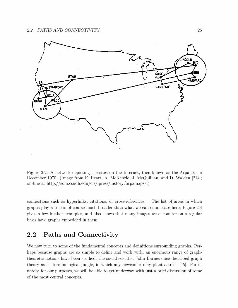
the toy examples in Figure 2.1 with a real example. Figure 2.2 depicts the network structure

of the Internet — then called the Arpanet — in December 1970 [214], when it had only 13

sites. Nodes represent computing hosts, and there is an edge joining two nodes in this picture

if there is a direct communication link between them. Ignoring the superimposed map of the

U.S. (and the circles indicating blown-up regions in Massachusetts and Southern California),

the rest of the image is simply a depiction of this 13-node graph using the same dots-and-lines

style that we saw in Figure 2.1. Note that for showing the pattern of connections, the actual

placement or layout of the nodes is immaterial; all that matters is which nodes are linked

to which others. Thus, Figure 2.3 shows a different drawing of the same 13-node Arpanet

graph.

Graphs appear in many domains, whenever it is useful to represent how things are either

physically or logically linked to one another in a network structure. The 13-node Arpanet in

Figures 2.2 and 2.3 is an example of a communication network, in which nodes are computers

or other devices that can relay messages, and the edges represent direct links along which

messages can be transmitted. In Chapter 1, we saw examples from two other broad classes of

graph structures: social networks, in which nodes are people or groups of people, and edges

represent some kind of social interaction; and information networks, in which the nodes

are information resources such as Web pages or documents, and edges represent logical

2.2. PATHS AND CONNECTIVITY 25

Figure 2.2: A network depicting the sites on the Internet, then known as the Arpanet, inDecember 1970. (Image from F. Heart, A. McKenzie, J. McQuillian, and D. Walden [214];on-line at http://som.csudh.edu/cis/lpress/history/arpamaps/.)

connections such as hyperlinks, citations, or cross-references. The list of areas in which

graphs play a role is of course much broader than what we can enumerate here; Figure 2.4

gives a few further examples, and also shows that many images we encounter on a regular

basis have graphs embedded in them.

2.2 Paths and Connectivity

We now turn to some of the fundamental concepts and definitions surrounding graphs. Per-

haps because graphs are so simple to define and work with, an enormous range of graph-

theoretic notions have been studied; the social scientist John Barnes once described graph

theory as a “terminological jungle, in which any newcomer may plant a tree” [45]. Fortu-

nately, for our purposes, we will be able to get underway with just a brief discussion of some

of the most central concepts.


LINC

CASE

CARN

HARV

BBN

MIT

SDC

RAND

UTAHSRI

UCLA

STANUCSB

Figure 2.3: An alternate drawing of the 13-node Internet graph from December 1970.

Paths. Although we’ve been discussing examples of graphs in many different areas, there

are clearly some common themes in the use of graphs across these areas. Perhaps foremost

among these is the idea that things often travel across the edges of a graph, moving from

node to node in sequence — this could be a passenger taking a sequence of airline flights, a

piece of information being passed from person to person in a social network, or a computer

user or piece of software visiting a sequence of Web pages by following links.

This idea motivates the definition of a path in a graph: a path is simply a sequence of

nodes with the property that each consecutive pair in the sequence is connected by an edge.

Sometimes it is also useful to think of the path as containing not just the nodes but also the

sequence of edges linking these nodes. For example, the sequence of nodes mit, bbn, rand,

ucla is a path in the Internet graph from Figures 2.2 and 2.3, as is the sequence case,

lincoln, mit, utah, sri, ucsb. As we have defined it here, a path can repeat nodes: for

example, sri, stan, ucla, sri, utah, mit is a path. But most paths we consider will not

do this; if we want to emphasize that the path we are discussing does not repeat nodes, we

can refer to it as a simple path.

Cycles. A particularly important kind of non-simple path is a cycle, which informally is a

“ring” structure such as the sequence of nodes linc, case, carn, harv, bbn, mit, linc

on the right-hand-side of Figure 2.3. More precisely, a cycle is a path with at least three

edges, in which the first and last nodes are the same, but otherwise all nodes are distinct.

There are many cycles in Figure 2.3: sri, stan, ucla, sri is as short an example as possible

according to our definition (since it has exactly three edges), while sri, stan, ucla, rand,

bbn, mit, utah, sri is a significantly longer example.

In fact, every edge in the 1970 Arpanet belongs to a cycle, and this was by design: it means

that if any edge were to fail (e.g. a construction crew accidentally cut through the cable),

there would still be a way to get from any node to any other node. More generally, cycles


(a) Airline routes (b) Subway map

(c) Flowchart of college courses (d) Tank Street Bridge in Brisbane

Figure 2.4: Images of graphs arising in different domains. The depictions of airline and subway systemsin (a) and (b) are examples of transportation networks, in which nodes are destinations and edges representdirect connections. Much of the terminology surrounding graphs derives from metaphors based on transporta-tion through a network of roads, rail lines, or airline flights. The prerequisites among college courses in (c) isan example of a dependency network, in which nodes are tasks and directed edges indicate that one task mustbe performed before another. The design of complex software systems and industrial processes often requiresthe analysis of enormous dependency networks, with important consequences for efficient scheduling in thesesettings. The Tank Street Bridge from Brisbane, Australia shown in (d) is an example of a structural network,with joints as nodes and physical linkages as edges. The internal frameworks of mechanical structures such asbuildings, vehicles, or human bodies are based on such networks, and the area of rigidity theory, at the inter-section of geometry and mechanical engineering, studies the stability of such structures from a graph-basedperspective [388]. (Images: (a) www.airlineroutemaps.com/USA/Northwest Airlines asia pacific.shtml, (b)www.wmata.com/metrorail/systemmap.cfm, (c) www.cs.cornell.edu/ugrad/flowchart.htm.)


F

GH

J

I

K

L

A

B

C

E

D

M

Figure 2.5: A graph with three connected components.

in communication and transportation networks are often present to allow for redundancy —

they provide for alternate routings that go the “other way” around the cycle. In the social

network of friendships too, we often notice cycles in everyday life, even if we don’t refer to

them as such. When you discover, for example, that your wife’s cousin’s close friend from

high school is in fact someone who works with your brother, this is a cycle — consisting

of you, your wife, her cousin, his high-school-friend, his co-worker (i.e. your brother), and

finally back to you.

Connectivity. Given a graph, it is natural to ask whether every node can reach every

other node by a path. With this in mind, we say that a graph is connected if for every pair of

nodes, there is a path between them. For example, the 13-node Arpanet graph is connected;

and more generally, one expects most communication and transportation networks to be

connected — or at least aspire to be connected — since their goal is to move traffic from

one node to another.

On the other hand, there is no a priori reason to expect graphs in other settings to be

connected — for example, in a social network, you could imagine that there might exist two

people for which it’s not possible to construct a path from one to the other. Figures 2.5

and 2.6 give examples of disconnected graphs. The first is a toy example, while the second

is built from the collaboration graph at a biological research center [134]: nodes represent


Figure 2.6: The collaboration graph of the biological research center Structural Genomics ofPathogenic Protozoa (SGPP) [134], which consists of three distinct connected components.This graph was part of a comparative study of the collaboration patterns graphs of nineresearch centers supported by NIH’s Protein Structure Initiative; SGPP was an intermediatecase between centers whose collaboration graph was connected and those for which it wasfragmented into many small components.

researchers, and there is an edge between two nodes if the researchers appear jointly on a

co-authored publication. (Thus the edges in this second figure represent a particular formal

definition of collaboration — joint authorship of a published paper — and do not attempt to

capture the network of more informal interactions that presumably take place at the research

center.)

Components. Figures 2.5 and 2.6 make visually apparent a basic fact about disconnected

graphs: if a graph is not connected, then it breaks apart naturally into a set of connected

“pieces,” groups of nodes so that each group is connected when considered as a graph in

isolation, and so that no two groups overlap. In Figure 2.5, we see that the graph consists

of three such pieces: one consisting of nodes A and B, one consisting of nodes C, D, and E,

and one consisting of the rest of the nodes. The network in Figure 2.6 also consists of three

pieces: one on three nodes, one on four nodes, and one that is much larger.

To make this notion precise, we we say that a connected component of a graph (often

shortened just to the term “component”) is a subset of the nodes such that: (i) every node

in the subset has a path to every other; and (ii) the subset is not part of some larger set

with the property that every node can reach every other. Notice how both (i) and (ii)


are necessary to formalize the intuitive definition: (i) says that the component is indeed

internally connected, and (ii) says that it really is a free-standing “piece” of the graph, not

a connected part of a larger piece. (For example, we would not think of the set of nodes F ,

G, H, and J in Figure 2.5 as forming a component, because this set violates part (ii) of the

definition: although there are paths among all pairs of nodes in the set, it belongs to the

larger set consisting of F -M , in which all pairs are also linked by paths.)

Dividing a graph into its components is of course only a first, global way of describing

its structure. Within a given component, there may be richer internal structure that is

important to one’s interpretation of the network. For example, thinking about the largest

component from Figure 2.6 in light of the collaborations that it represents, one notices certain

suggestive features of the structure: a prominent node at the center, and tightly-knit groups

linked to this node but not to each other. One way to formalize the role of the prominent

central node is to observe that the largest connected component would break apart into three

distinct components if this node were removed. Analyzing a graph this way, in terms of its

densely-connected regions and the boundaries between them, is a powerful way of thinking

about network structure, and it will be a central topic in Chapter 3.

Giant Components. There turns out to be a useful qualitative way of thinking about

the connected components of typical large networks, and for this it helps to begin with the

following thought experiment. Consider the social network of the entire world, with a link

between two people if they are friends. Now, of course, this is a graph that we don’t actually

have explicitly recorded anywhere, but it is one where we can use our general intuitions to

answer some basic questions.

First, is this global friendship network connected? Presumably not. After all, connec-

tivity is a fairly brittle property, in that the behavior of a single node (or a small set of

nodes) can negate it. For example, a single person with no living friends would constitute

a one-node component in the global friendship network, and hence the graph would not be

connected. Or the canonical “remote tropical island,” consisting of people who have had

no contact with the outside world, would also be a small component in the network, again

showing that it is not connected.

But there is something more going on here. If you’re a typical reader of this book, then

you have friends who grew up in other countries. You’re in the same component as all these

friends, since you have a path (containing a single edge) to each of them. Now, if you consider,

say, the parents of these friends, your friends’ parents’ friends, their friends and descendants,

then all of these people are in the same component as well — and by now, we’re talking

about people who have never heard of you, may well not share a language with you, may

have never traveled anywhere near where you live, and may have had enormously different

life experiences. So even though the global friendship network may not be connected, the


component you inhabit seems very large indeed — it reaches into most parts of the world,

includes people from many different backgrounds, and seems in fact likely to contain a

significant fraction of the world’s population.

This is in fact true when one looks across a range of network datasets — large, complex

networks often have what is called a giant component, a deliberately informal term for a

connected component that contains a significant fraction of all the nodes. Moreover, when

a network contains a giant component, it almost always contains only one. To see why, let’s

go back to the example of the global friendship network and try imagining that there were

two giant components, each with hundreds of millions of people. All it would take is a single

edge from someone in the first of these components to someone in the second, and the two

giant components would merge into a single component. Just a single edge — in most cases,

it’s essentially inconceivable that some such edge wouldn’t form, and hence two co-existing

giant components are something one almost never sees in real networks. When there is a

giant component, it is thus generally unique, distinguishable as a component that dwarfs all

others.

In fact, in some of the rare cases when two giant components have co-existed for a long

time in a real network, their merging has been sudden, dramatic, and ultimately catastrophic.

For example, Jared Diamond’s book Guns, Germs, and Steel [130] devotes much of its

attention to the cataclysm that befell the civilizations of the Western hemisphere when

European explorers began arriving in it roughly half a millenium ago. One can view this

development from a network perspective as follows: five thousand years ago, the global

social network likely contained two giant components — one in the Americas, and one in

the Europe-Asia land mass. Because of this, technology evolved independently in the two

components, and perhaps even worse, human diseases evolved independently; and so when

the two components finally came in contact, the technology and diseases of one quickly and

disastrously overwhelmed the other.

The notion of giant components is useful for reasoning about networks on much smaller

scales as well. The collaboration network in Figure 2.6 is one simple example; another

interesting example is depicted in Figure 2.7, which shows the romantic relationships in an

American high school over an 18-month period [49]. (These edges were not all present at

once; rather, there is an edge between two people if they were romantically involved at any

point during the time period.) The fact that this graph contains such a large component is

significant when one thinks about the spread of sexually transmitted diseases, a focus of the

researchers performing the study. A high-school student may have had a single partner over

this time period and nevertheless — without realizing it — be part of this large component

and hence part of many paths of potential transmission. As Bearman, Moody, and Stovel

note in the paper where they analyze this network, “These structures reflect relationships

that may be long over, and they link individuals together in chains far too long to be


Figure 2.7: A network in which the nodes are students in a large American high school, andan edge joins two who had a romantic relationship at some point during the 18-month periodin which the study was conducted [49].

the subject of even the most intense gossip and scrutiny. Nevertheless, they are real: like

social facts, they are invisible yet consequential macrostructures that arise as the product of

individual agency.”

2.3 Distance and Breadth-First Search

In addition to simply asking whether two nodes are connected by a path, it is also interesting

in most settings to ask how long such a path is — in transportation, Internet communication,

or the spread of news and diseases, it is often important whether something flowing through

a network has to travel just a few hops or many.

To be able to talk about this notion precisely, we define the length of a path to be the

number of steps it contains from beginning to end — in other words, the number of edges

in the sequence that comprises it. Thus, for example, the path mit, bbn, rand, ucla in

Figure 2.3 has length three, while the path mit, utah has length one. Using the notion of

2.3. DISTANCE AND BREADTH-FIRST SEARCH 33

you

distance 1

distance 2

distance 3

your friends

friends of friends

friends of friends

of friends

all nodes, not already discovered, that have an

edge to some node in the previous layer

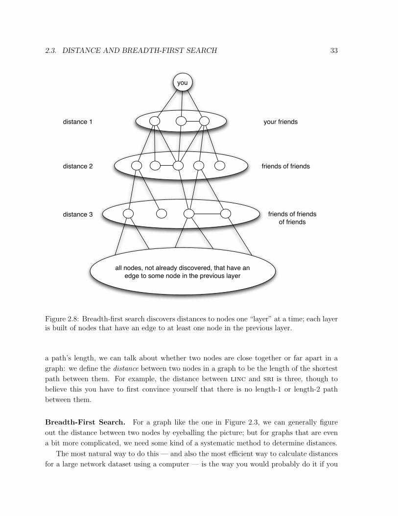
Figure 2.8: Breadth-first search discovers distances to nodes one “layer” at a time; each layeris built of nodes that have an edge to at least one node in the previous layer.

a path’s length, we can talk about whether two nodes are close together or far apart in a

graph: we define the distance between two nodes in a graph to be the length of the shortest

path between them. For example, the distance between linc and sri is three, though to

believe this you have to first convince yourself that there is no length-1 or length-2 path

between them.

Breadth-First Search. For a graph like the one in Figure 2.3, we can generally figure

out the distance between two nodes by eyeballing the picture; but for graphs that are even

a bit more complicated, we need some kind of a systematic method to determine distances.

The most natural way to do this — and also the most efficient way to calculate distances

for a large network dataset using a computer — is the way you would probably do it if you


LINC

CASE

CARN

HARV

BBN

MIT

SDC RAND

UTAH

SRI

UCLASTANUCSB

distance 1

distance 2

distance 3

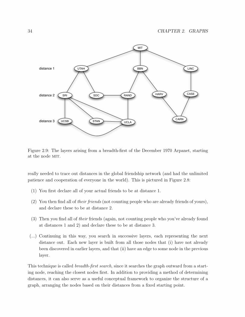
Figure 2.9: The layers arising from a breadth-first of the December 1970 Arpanet, startingat the node mit.

really needed to trace out distances in the global friendship network (and had the unlimited

patience and cooperation of everyone in the world). This is pictured in Figure 2.8:

(1) You first declare all of your actual friends to be at distance 1.

(2) You then find all of their friends (not counting people who are already friends of yours),

and declare these to be at distance 2.

(3) Then you find all of their friends (again, not counting people who you’ve already found

at distances 1 and 2) and declare these to be at distance 3.

(...) Continuing in this way, you search in successive layers, each representing the next

distance out. Each new layer is built from all those nodes that (i) have not already

been discovered in earlier layers, and that (ii) have an edge to some node in the previous

layer.

This technique is called breadth-first search, since it searches the graph outward from a start-

ing node, reaching the closest nodes first. In addition to providing a method of determining

distances, it can also serve as a useful conceptual framework to organize the structure of a

graph, arranging the nodes based on their distances from a fixed starting point.


Of course, despite the social-network metaphor we used to describe breadth-first search,

the process can be applied to any graph: one just keeps discovering nodes layer-by-layer,

building each new layer from the nodes that are connected to at least one node in the previous

layer. For example, Figure 2.9 shows how to discover all distances from the node mit in the

13-node Arpanet graph from Figure 2.3.

The Small-World Phenomenon. As with our discussion of the connected components

in a graph, there is something qualitative we can say, beyond the formal definitions, about

distances in typical large networks. If we go back to our thought experiments on the global

friendship network, we see that the argument explaining why you belong to a giant compo-

nent in fact asserts something stronger: not only do you have paths of friends connecting

you to a large fraction of the world’s population, but these paths are surprisingly short.

Take the example of a friend who grew up in another country: following a path through this

friend, to his or her parents, to their friends, you’ve followed only three steps and ended up

in a different part of the world, in a different generation, with people who have very little in

common with you.

This idea has been termed the small-world phenomenon — the idea that the world looks

“small” when you think of how short a path of friends it takes to get from you to almost

anyone else. It’s also known, perhaps more memorably, as the six degrees of separation; this

phrase comes from the play of this title by John Guare [200], and in particular from the line

uttered by one of the play’s characters: “I read somewhere that everybody on this planet is

separated by only six other people. Six degrees of separation between us and everyone else

on this planet.”

The first experimental study of this notion — and the origin of the number “six” in the

pop-cultural mantra — was performed by Stanley Milgram and his colleagues in the 1960s

[297, 391]. Lacking any of the massive social-network datasets we have today, and with a

budget of only $680, he set out to test the speculative idea that people are really connected in

the global friendship network by short chains of friends. To this end, he asked a collection of

296 randomly chosen “starters” to try forwarding a letter to a “target” person, a stockbroker

who lived in a suburb of Boston. The starters were each given some personal information

about the target (including his address and occupation) and were asked to forward the

letter to someone they knew on a first-name basis, with the same instructions, in order to

eventually reach the target as quickly as possible. Each letter thus passed through the hands

of a sequence of friends in succession, and each thereby formed a chain of people that closed

in on the stockbroker outside Boston.

Figure 2.10 shows the distribution of path lengths, among the 64 chains that succeeded

in reaching the target; the median length was six, the number that made its way two decades

later into the title of Guare’s play. That so many letters reached their destination, and by


Figure 2.10: A histogram from Travers and Milgram’s paper on their small-world experiment[391]. For each possible length (labeled “number of intermediaries” on the x-axis), the plotshows the number of successfully completed chains of that length. In total, 64 chains reachedthe target person, with a median length of six.

such short paths, was a striking fact when it was first discovered, and it remains so today.

Of course, it is worth noting a few caveats about the experiment. First, it clearly doesn’t

establish a statement quite as bold as “six degrees of separation between us and everyone

else on this planet” — the paths were just to a single, fairly affluent target; many letters

never got there; and attempts to recreate the experiment have been problematic due to lack

of participation [255]. Second, one can ask how useful these short paths really are to people

in society: even if you can reach someone through a short chain of friends, is this useful to

you? Does it mean you’re truly socially “close” to them? Milgram himself mused about this

in his original paper [297]; his observation, paraphrased slightly, was that if we think of each

person as the center of their own social “world,” then “six short steps” becomes “six worlds

apart” — a change in perspective that makes six sound like a much larger number.

Despite these caveats, the experiment and the phenomena that it hints at have formed

a crucial aspect in our understanding of social networks. In the years since the initial

experiment, the overall conclusion has been accepted in a broad sense: social networks tend

to have very short paths between essentially arbitrary pairs of people. And even if your six-


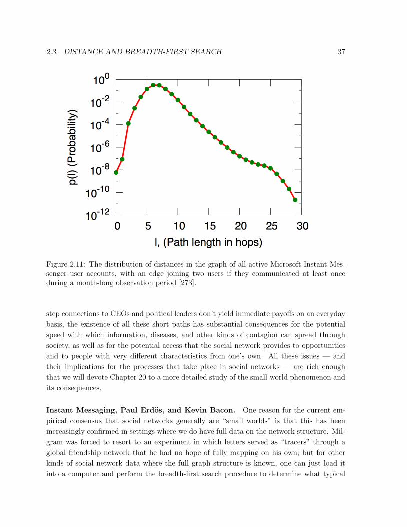
Figure 2.11: The distribution of distances in the graph of all active Microsoft Instant Mes-senger user accounts, with an edge joining two users if they communicated at least onceduring a month-long observation period [273].

step connections to CEOs and political leaders don’t yield immediate payoffs on an everyday

basis, the existence of all these short paths has substantial consequences for the potential

speed with which information, diseases, and other kinds of contagion can spread through

society, as well as for the potential access that the social network provides to opportunities

and to people with very different characteristics from one’s own. All these issues — and

their implications for the processes that take place in social networks — are rich enough

that we will devote Chapter 20 to a more detailed study of the small-world phenomenon and

its consequences.

Instant Messaging, Paul Erdos, and Kevin Bacon. One reason for the current em-

pirical consensus that social networks generally are “small worlds” is that this has been

increasingly confirmed in settings where we do have full data on the network structure. Mil-

gram was forced to resort to an experiment in which letters served as “tracers” through a

global friendship network that he had no hope of fully mapping on his own; but for other

kinds of social network data where the full graph structure is known, one can just load it

into a computer and perform the breadth-first search procedure to determine what typical


Figure 2.12: Ron Graham’s hand-drawn picture of a part of the mathematics collaborationgraph, centered on Paul Erdos [189]. (Image from http://www.oakland.edu/enp/cgraph.jpg)

distances look like.

One of the largest such computational studies was performed by Jure Leskovec and Eric

Horvitz [273]. They analyzed the 240 million active user accounts on Microsoft Instant

Messenger, building a graph in which each node corresponds to a user, and there is an

edge between two users if they engaged in a two-way conversation at any point during a

month-long observation period. As employees of Microsoft at the time, they had access to

a complete snapshot of the system for the month under study, so there were no concerns

about missing data. This graph turned out to have a giant component containing almost

all of the nodes, and the distances within this giant component were very small. Indeed,

the distances in the Instant Messenger network closely corresponded to the numbers from

Milgram’s experiment, with an estimated average distance of 6.6, and an estimated median


of seven. Figure 2.11 shows the distribution of distances averaged over a random sample

of 1000 users: breadth-first search was performed separately from each of these 1000 users,

and the results from these 1000 nodes were combined to produce the plot in the figure.

The reason for this estimation by sampling users is a computational one: the graph was

so large that performing breadth-first search from every single node would have taken an

astronomical amount of time. Producing plots like this efficiently for massive graphs is an

interesting research topic in itself [338].

In a sense, the plot in Figure 2.11 starts to approximate, in a striking way, what Milgram

and his colleagues were trying to understand — the distribution of how far apart we all are

in the full global friendship network. At the same time, reconciling the structure of such

massive datasets with the underlying networks they are trying to measure is an issue that

comes up here, as it will many times throughout the book. In this case, enormous as the

Microsoft IM study was, it remains some distance away from Milgram’s goal: it only tracks

people who are technologically-endowed enough to have access to instant messaging, and

rather than basing the graph on who is truly friends with whom, it can only observe who

talks to whom during an observation period.

Turning to a smaller scale — at the level of hundred of thousands of people rather than

hundreds of millions — researchers have also discovered very short paths in the collaboration

networks within professional communities. In the domain of mathematics, for example,

people often speak of the itinerant mathematician Paul Erdos — who published roughly

1500 papers over his career — as a central figure in the collaborative structure of the field.

To make this precise, we can define a collaboration graph as we did for Figure 2.6, in this

case with nodes corresponding to mathematicians, and edges connecting pairs who have

jointly authored a paper. (While Figure 2.6 concerned a single research lab, we are now

talking about collaboration within the entire field of mathematics.) Figure 2.12 shows a

small hand-drawn piece of the collaboration graph, with paths leading to Paul Erdos [189].

Now, a mathematician’s Erdos number is the distance from him or her to Erdos in this graph

[198]. The point is that most mathematicians have Erdos numbers of at most 4 or 5, and —

extending the collaboration graph to include co-authorship across all the sciences — most

scientists in other fields have Erdos numbers that are comparable or only slightly larger;

Albert Einstein’s is 2, Enrico Fermi’s is 3, Noam Chomsky’s and Linus Pauling’s are each 4,

Francis Crick’s and James Watson’s are 5 and 6 respectively. The world of science is truly

a small one in this sense.

Inspired by some mixture of the Milgram experiment, John Guare’s play, and a compelling

belief that Kevin Bacon was the center of the Hollywood universe, three students at Albright

College in Pennsylvania sometime around 1994 adapted the idea of Erdos numbers to the

collaboration graph of movie actors and actresses: nodes are performers, an edge connects

two performers if they’ve appeared together in a movie, and a performer’s Bacon number is


his or her distance in this graph to Kevin Bacon [372]. Using cast lists from the Internet

Movie Database (IMDB), it is possible to compute Bacon numbers for all performers via

breadth-first search — and as with mathematics, it’s a small world indeed. The average

Bacon number, over all performers in the IMDB, is approximately 2.9, and it’s a challenge

to find one that’s larger than 5. Indeed, it’s fitting to conclude with a network-and-movie

enthusiast’s description of his late-night attempts to find the largest Bacon number in the

IMDB by hand: “With my life-long passion for movies, I couldn’t resist spending many

hours probing the dark recesses of film history until, at about 10 AM on Sunday, I found an

incredibly obscure 1928 Soviet pirate film, Plenniki Morya, starring P. Savin with a Bacon

number of 7, and whose supporting cast of 8 appeared nowhere else” [197]. One is left with

the image of a long exploration that arrives finally at the outer edge of the movie world —

in the early history of film, in the Soviet Union — and yet in another sense, only 8 steps

from where it started.

2.4 Network Datasets: An Overview

The explosion of research on large-scale networks in recent years has been fueled to a large

extent by the increasing availability of large, detailed network datasets. We’ve seen examples

of such datasets throughout these first two chapters, and it’s useful at this point to step

back and think more systematically about where people have been getting the data that

they employ in large-scale studies of networks.

To put this in perspective, we note first of all that there are several distinct reasons

why you might study a particular network dataset. One is that you may care about the

actual domain it comes from, so that fine-grained details of the data itself are potentially

as interesting as the broad picture. Another is that you’re using the dataset as a proxy

for a related network that may be impossible to measure — as for example in the way

the Microsoft IM graph from Figure 2.11 gave us information about distances in a social

network of a scale and character that begins to approximate the global friendship network.

A third possibility is that you’re trying to look for network properties that appear to be

common across many different domains, and so finding a similar effect in unrelated settings

can suggest that it has a certain universal nature, with possible explanations that are not

tied to the specifics of any one of the domains.

Of course, all three of these motivations are often at work simultaneously, to varying

degrees, in the same piece of research. For example, the analysis of the Microsoft IM graph

gave us insight into the global friendship network — but at a more specific level, the re-

searchers performing the study were also interested in the dynamics of instant messaging

in particular; and at a more general level, the result of the IM graph analysis fit into the

broader framework of small-world phenomena that span many domains.

2.4. NETWORK DATASETS: AN OVERVIEW 41

As a final point, we’re concerned here with sources of data on networks that are large.

If one wants to study a social network on 20 people — say, within a small company, or a

fraternity or sorority, or a karate club as in Figure 1.1 — then one strategy is to interview

all the people involved and ask them who their friends are. But if we want to study the

interactions among 20,000 people, or 20,000 individual nodes of some other kind, then we

need to be more opportunistic in where we look for data: except in unusual cases, we can’t

simply go out and collect everything by hand, and so we need to think about settings in

which the data has in some essential way already been measured for us.

With this in mind, let’s consider some of the main sources of large-scale network data

that people have used for research. The resulting list is far from exhaustive, nor are the

categories truly distinct — a single dataset can easily exhibit characteristics from several.

• Collaboration Graphs. Collaboration graphs record who works with whom in a specific

setting; co-authorships among scientists and co-appearance in movies by actors and

actresses are two examples of collaboration graphs that we discussed in Section 2.3.

Another example that has been extensively studied by sociologists is the graph on

highly-placed people in the corporate world, with an edge joining two if they have

served together on the board of directors of the same Fortune 500 company [301]. The

on-line world provides new instances: the Wikipedia collaboration graph (connecting

two Wikipedia editors if they’ve ever edited the same article) [122, 246] and the World-

of-Warcraft collaboration graph (connecting two W-o-W users if they’ve ever taken part

together in the same raid or other activity) [419] are just two examples.

Sometimes a collaboration graph is studied to learn about the specific domain it comes

from; for example, sociologists who study the business world have a substantive in-

terest in the relationships among companies at the director level, as expressed via

co-membership on boards. On the other hand, while there is a research community

that studies the sociological context of scientific research, a broader community of

people is interested in scientific co-authorship networks precisely because they form

detailed, pre-digested snapshots of a rich form of social interaction that unfolds over a

long period of time [318]. By using on-line bibliographic records, one can often track

the patterns of collaboration within a field across a century or more, and thereby at-

tempt to extrapolate how the social structure of collaboration may work across a range

of harder-to-measure settings as well.

• Who-talks-to-Whom Graphs. The Microsoft IM graph is a snapshot of a large commu-

nity engaged in several billion conversations over the course of a month. In this way,

it captures the “who-talks-to-whom” structure of the community. Similar datasets

have been constructed from the e-mail logs within a company [6] or a university [259],

as well as from records of phone calls: researchers have studied the structure of call


graphs in which each node is a phone number, and there is an edge between two if they

engaged in a phone call over a given observation period [1, 334]. One can also use the

fact that mobile phones with short-range wireless technology can detect other similar

devices nearby. By equipping a group of experimental subjects with such devices and

studying the traces they record, researchers can thereby build “face-to-face” graphs

that record physical proximity: a node in such a graph is a person carrying one of the

mobile devices, and there is an edge joining two people if they were detected to be in

close physical proximity over a given observation period [141, 142].

In almost all of these kinds of datasets, the nodes represent customers, employees, or

students of the organization that maintains the data. These individuals will generally

have strong expectations of privacy, not necessarily even appreciating how easily one

can reconstruct details of their behavior from the digital traces they leave behind

when communicating by e-mail, instant messaging, or phone. As a result, the style of

research performed on this kind of data is generally restricted in specific ways so as to

protect the privacy of the individuals in the data. Such privacy considerations have

also become a topic of significant discussion in settings where companies try to use this

type of data for marketing, or when governments try to use it for intelligence-gathering

purposes [315].

Related to this kind of “who-talks-to-whom” data, economic network measurements

recording the “who-transacts-with-whom” structure of a market or financial commu-

nity has been used to study the ways in which different levels of access to market

participants can lead to different levels of market power and different prices for goods.

This empirical work has in turn motivated more mathematical investigations of how

a network structure limiting access between buyers and sellers can affect outcomes

[63, 176, 232, 261], a focus of discussion in Chapters 10—12.

• Information Linkage Graphs. Snapshots of the Web are central examples of network

datasets; nodes are Web pages and directed edges represent links from one page to

another. Web data stands out both in its scale and in the diversity of what the nodes

represent: billions of little pieces of information, with links wiring them together. And

clearly it is not just the information that is of interest, but the social and economic

structures that stand behind the information: hundreds of millions of personal pages on

social-networking and blogging sites, hundreds of millions more representing companies

and governmental organizations trying to engineer their external images in a crowded

network.

A network on the scale of the full Web can be daunting to work with; simply manipu-

lating the data effectively can become a research challenge in itself. As a result, much

network research has been done on interesting, well-defined subsets of the Web, includ-

2.4. NETWORK DATASETS: AN OVERVIEW 43

ing the linkages among bloggers [264], among pages on Wikipedia [404], among pages

on social-networking sites such as Facebook or MySpace [185], or among discussions

and product reviews on shopping sites [201].

The study of information linkage graphs significantly predates the Web: the field of

citation analysis has, since the early part of the 20th century, studied the network

structure of citations among scientific papers or patents, as a way of tracking the

evolution of science [145]. Citation networks are still popular research datasets today,

for the same reason that scientific co-authorship graphs are: even if you don’t have a

substantive interest in the social processes by which science gets done, citation networks

are very clean datasets that can easily span many decades.

• Technological Networks. Although the Web is built on a lot of sophisticated technology,

it would be a mistake to think of it primarily as a technological network: it is really a

projection onto a technological backdrop of ideas, information, and social and economic

structure created by humans. But as we noted in the opening chapter, there has

clearly been a convergence of social and technological networks over recent years, and

much interesting network data comes from the more overtly technological end of the

spectrum — with nodes representing physical devices and edges representing physical

connections between them. Examples include the interconnections among computers

on the Internet [155] or among generating stations in a power grid [411].

Even physical networks like these are ultimately economic networks as well, represent-

ing the interactions among the competing organizations, companies, regulatory bodies,

and other economic entities that shape it. On the Internet, this is made particularly

explicit by a two-level view of the network. At the lowest level, nodes are individual

routers and computers, with an edge meaning that two devices actually have a physical

connection to each other. But at a higher level, these nodes are grouped into what are

essentially little “nation-states” termed autonomous systems, each one controlled by a

different Internet service-providers. There is then a who-transacts-with-whom graph

on the autonomous systems, known as the AS graph, that represents the data transfer

agreements these Internet service-providers make with each other.

• Networks in the Natural World. Graph structures also abound in biology and the

other natural sciences, and network research has devoted particular attention to several

different types of biological networks. Here are three examples at three different scales,

from the population level down to the molecular level.

As a first example, food webs represent the who-eats-whom relationships among species

in an ecosystem [137]: there is a node for each species, and a directed edge from node

A to node B indicates that members of A consume members of B. Understanding

the structure of a food web as a graph can help in reasoning about issues such as


cascading extinctions: if certain species become extinct, then species that rely on them

for food risk becoming extinct as well, if they do not have alternative food sources;

these extinctions can propagate through the food web as a chain reaction.

Another heavily-studied network in biology is the structure of neural connections within

an organism’s brain: the nodes are neurons, and an edge represents a connection

between two neurons [380]. The global brain architecture for simple organisms like

C. Elegans, with 302 nodes and roughly 7000 edges, has essentially been completely

mapped [3]; but obtaining a detailed network picture for brains of “higher” organisms is

far beyond the current state of the art. However, significant insight has been gained by

studying the structure of specific modules within a complex brain, and understanding

how they relate to one another.

A final example is the set of networks that make up a cell’s metabolism. There are

many ways to define these networks, but roughly, the nodes are compounds that play

a role in a metabolic process, and the edges represent chemical interactions among

them [43]. There is considerable hope that analysis of these networks can shed light

on the complex reaction pathways and regulatory feedback loops that take place inside

a cell, and perhaps suggest “network-centric” attacks on pathogens that disrupt their

metabolism in targeted ways.

2.5 Exercises

1. One reason for graph theory’s power as a modeling tool is the fluidity with which

one can formalize properties of large systems using the language of graphs, and then

systematically explore their consequences. In this first set of questions, we will work

through an example of this process using the concept of a pivotal node.

First, recall from Chapter 2 that a shortest path between two nodes is a path of the

minimum possible length. We say that a node X is pivotal for a pair of distinct nodes

Y and Z if X lies on every shortest path between Y and Z (and X is not equal to

either Y or Z).

For example, in the graph in Figure 2.13, node B is pivotal for two pairs: the pair

consisting of A and C, and the pair consisting of A and D. (Notice that B is not

pivotal for the pair consisting of D and E since there are two different shortest paths

connecting D and E, one of which (using C and F ) doesn’t pass through B. So B

is not on every shortest path between D and E.) On the other hand, node D is not

pivotal for any pairs.

(a) Give an example of a graph in which every node is pivotal for at least one pair of

nodes. Explain your answer.

2.5. EXERCISES 45

B

A

C D

E

F

Figure 2.13: In this example, node B is pivotal for two pairs: the pair consisting of A andC, and the pair consisting of A and D. On the other hand, node D is not pivotal for anypairs.

(b) Give an example of a graph in which every node is pivotal for at least two different

pairs of nodes. Explain your answer.

(c) Give an example of a graph having at least four nodes in which there is a single

node X that is pivotal for every pair of nodes (not counting pairs that include

X). Explain your answer.

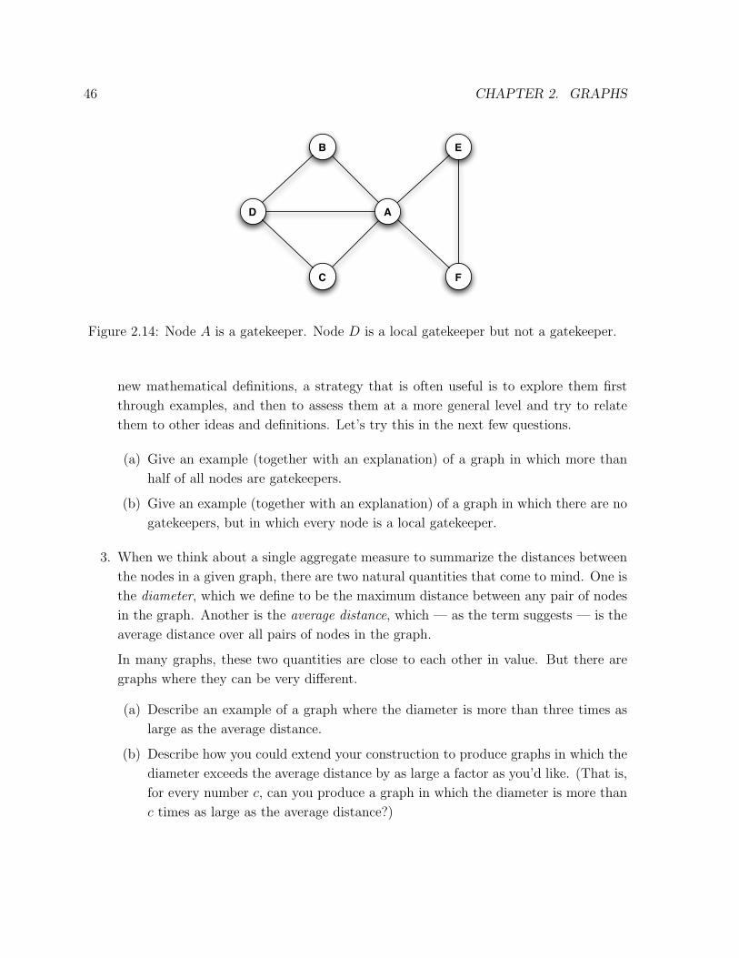
2. In the next set of questions, we consider a related cluster of definitions, which seek to

formalize the idea that certain nodes can play a “gatekeeping” role in a network. The

first definition is the following: we say that a node X is a gatekeeper if for some other

two nodes Y and Z, every path from Y to Z passes through X. For example, in the

graph in Figure 2.14, node A is a gatekeeper, since it lies for example on every path

from B to E. (It also lies on every path between other pairs of nodes — for example,

the pair D and E, as well as other pairs.)

This definition has a certain “global” flavor, since it requires that we think about paths

in the full graph in order to decide whether a particular node is a gatekeeper. A more

“local” version of this definition might involve only looking at the neighbors of a node.

Here’s a way to make this precise: we say that a node X is a local gatekeeper if there

are two neighbors of X, say Y and Z, that are not connected by an edge. (That is,

for X to be a local gatekeeper, there should be two nodes Y and Z so that Y and Z

each have edges to X, but not to each other.) So for example, in Figure 2.14, node

A is a local gatekeeper as well as being a gatekeeper; node D, on the other hand, is a

local gatekeeper but not a gatekeeper. (Node D has neighbors B and C that are not

connected by an edge; however, every pair of nodes — including B and C — can be

connected by a path that does not go through D.)

So we have two new definitions: gatekeeper, and local gatekeeper. When faced with


A

B

D

E

C F

Figure 2.14: Node A is a gatekeeper. Node D is a local gatekeeper but not a gatekeeper.

new mathematical definitions, a strategy that is often useful is to explore them first

through examples, and then to assess them at a more general level and try to relate

them to other ideas and definitions. Let’s try this in the next few questions.

(a) Give an example (together with an explanation) of a graph in which more than

half of all nodes are gatekeepers.

(b) Give an example (together with an explanation) of a graph in which there are no

gatekeepers, but in which every node is a local gatekeeper.

3. When we think about a single aggregate measure to summarize the distances between

the nodes in a given graph, there are two natural quantities that come to mind. One is

the diameter, which we define to be the maximum distance between any pair of nodes

in the graph. Another is the average distance, which — as the term suggests — is the

average distance over all pairs of nodes in the graph.

In many graphs, these two quantities are close to each other in value. But there are

graphs where they can be very different.

(a) Describe an example of a graph where the diameter is more than three times as

large as the average distance.

(b) Describe how you could extend your construction to produce graphs in which the

diameter exceeds the average distance by as large a factor as you’d like. (That is,

for every number c, can you produce a graph in which the diameter is more than

c times as large as the average distance?)

chapter 2 graphs - stanford university

Documents