CHAPTER 2

PSO BASED ECONOMIC LOAD DISPATCH PROBLEMS

2.1. INTRODUCTION

The main aim of electric power utilities is to provide high-quality. reliable

power supply to the consumers at the lowest possible cost while operating to meet the

limits and constraints imposed on the generating units. This formulates the economic

load dispatch (ELD) problem for finding the optimal combination of the output power

of all the online generating units that minimizes the total fuel cost, while satisfying an

equality constraint and a set of inequality constraints. As the cost of power generation

is exorbitant, an optimum dispatch results in economy.

In recent years, with an increasing awareness of the environmental pollution

caused by thermal power plants, limiting the emission of pollutants is becoming a

crucial issue in economic power dispatch. The conventional economic power dispatch

cannot meet the environmental protection requirements, since it only considers

minimizing the total fuel cost. The multiobjective generation dispatch in electric

power systems treats economic and emission impact as competing objectives, which

requires some reasonable tradeoff among objectives to reach an optimal solution. This

formulates the combined economic emission dispatch (CEED) problem with an

ohjective to dispatch the electric power considering both economic and environmental

concerns.

Practically, the real world input4utput characteristics of the generating units

are highly nonlinear, nonsmooth and discrete in nature owing to prohibited operating

zones, ramp rate limits and multifuel effects. Thus the resultant ELD is a challenging

nonconvex optimization problem, which is difficult lo solve using the traditional

methods.

In this work, particle swarm optimization (PSO) algorithm is proposed to

solve the various t)ipes of economic load dispatch problems in power systems such as

economic load dispatch (ELD) for combined cycle cogeneration plant (CCCP),

combined economic emission dispatch (CEED) and the economic load dispatch

(ELD) with prohibited operating zones considering ramp rate limits. The feasibility of

the proposed method is demonstrated on six different systems and the numerical

results were compared with classical and other evolut~onary computing techniques.

2.2. ECONOMIC LOAD DISPATCH PROBLEM

2.2.1. Problem Description

Economic load dispatch problem is the sub problem of optimal power flow

(OPF). The main objective of ELD is to minimize the fuel cost while satisfying the

load demand with transmission constraints.

2.2.2. Objective Function

The classical ELD with power balance and generation limit constraints has

been formulated [82] as follows.

d

Minimize F, = IF, (P,) 1-1

where Ft is the total fuel cost of generation,

F,(P,) is the fuel cost function of ith generator,

a,, b,, c, are the cost coefficients of ith generator,

P, is the real power generation of ith generator,

d represents the number of generators connected in the network

The minimum value of the above objective function has to be found by satisfytng the

following consh.aints.

The power balance constraint [82] d

CP, =Po +PL (2.3) i-I

where Po is the total load of the system and

PL is the transmission losses of the system.

The total transmission loss [83]

where P,,, and P,,, are the real power injections at mth and nth buses and

B, are the B-coefficients of transmission loss formula.

The inequality constraint on real power generation P, for each generator [82] is

P,"" 5 P, 5 P,"" (2.5)

where P , " " h d PIm' are, respect~vely, mlnlmum and maxlmum values of real

power allowed at generator I.

A. Economic Load Dispatch Problem with CCCP

Cogeneration units play an increasingly important role in the utility industry.

The mutual dependencies of the multiple demand and heat-power capacity of the

cogeneration units introduce a complication of integrating the system for economic

power dispatch. The cost characteristics of CCCP system (two 75 MW gas turbines

and one 50 MW steam turbine) [82] is obtained and hence can be found that they are

not differentiable. So the lambda-iterative method will fail in obtaining solution for

the ELD of the above problem. The solution for this problem is obtained by

formulating the cost equations by curve fitting technique and implementing the

proposed PSO algorithm for the optimal scheduling of generators.

B. Constraint Satisfaction Technique

To satisfy the equality constraint of equation (2.3). loading of any one of the

units is selected as the dependent loading Pdu, and its present value is replaced by the

value calculated according to the following equation [83]:

where, Pdu can be calculated directly from the equation (2.6) with the known power

demand PD and the known values of remaining loading of the generators. Therefore,

the dispatch solution always satisfies the power balance constraint provided that Pd.

also satisfies the operation limit constraint as given in equation (2.5). An infeasible

solution is omitted and above procedure is repeated until Pd. lies within its operational

limit. As PL also depends on Pdur an expression for Pl can be substituted in terms of

PI. Pz ,..., Pdu ..... Pd and B,, coefficients. After substituting PI in the equation (2.6).

the independent and dependent generator terms are separated to obtain a quadratic

equation for Pa.. The power balance equality condition is exactly met by solving the

quadratic equation for I'd,,.

2.2.3. Features of Particle Swarm Optimization (PSO)

Particle swarm optimization was first introduced by Kennedy and Eberhart in

the year 1995 [5]. It is an exciting new methodology in evolutionary computation and

a population-based optimization tool like GA. PSO is motivated from the simulation

of the behaviour of social systems such as fish schooling and birds flocking [84]. The

PSO algorithm requires less computation time and less memory because of its

inherent simplicity. The basic assumption behind the PSO algorithm is that birds find

food by flocking and not individually. This leads to the assumption that information is

owned jointly in the flocking. The swarm initially has a population of random

solutions. Each potential solution, called a particle (agent), is given a random velocity

and is flown through the problem space. All the particles have memory and each

particle keeps track of its previous best position @best) and the corresponding fitness

value. The swarm has another value called gbest, which is the best value of all the

pbest. Particle swarm optimization has been found to be extremely effective

in solving a wide range of eng~neering problems and solves them very quickly.

In a PSO system, population of part~cles exists in the n-dimensional search

space. Each particle has certain amount of knowledge and will move about the search

space on the basis of this knowledge. The particle has some inertia attributed to it and

hence will continue to have a component of motion in the direction it is moving. The

knows its location in the search space and will encounter with the best

solution. The particle will then modify its d~rection such that it has additional

components towards its own best position, pbest and towards the overall best position,

gbest. The particle updates its velocity [64] and position [64] using the following

equations (2.7) and (2.8)

where V: is the velocity of individual i at iterat~on k

k is pointer of iterations,

W is the weighing factor,

c l , c2 are the acceleration coefficients,

Randl( ), Rand2( ) are the random numbers between 0 and 1,

S: is the current position of individual i at iteration k,

pbest, is the best position of individual i

gbest is the best position of the group

In equation (2.7), cl has a range (1.5,2), which is called self-confidence range;

cz has a range (2, 2.5), which is called swarm range. The coefficients c , and cz pull

each particle towards pbest and gbest positions. Low values of acceleration

coefficients allow particles to roam far from the target regions, before being tugged

back. On the other hand, high values result in abrupt movement towards or past the

target regions. Hence, the acceleration coefficients cl and CI are often set to be 2

according to past experiences. The term c,Rand, ( ) x (pbest, - S f ) is called particle

memory influence or cognition part which represents the private thinking of the

itself and the term c,Rand,( ) x (gbest - S: ) is called swarm influence or the

social part which represents the collaboration among the particles.

In the procedure of the particle swarm paradigm, the value of maximum

allowed particle velocity Vm determines the resolution, or fitness, with which

regions are to be searched between the present position and the target position. If Vm"

is too high, particles may fly past good solutions. If V""" is too small, particles may

not explore sufficiently beyond local solutions. Thus, the system parameter VmX has

the beneficial effect of preventing explosion and scales the exploration of the particle

search. The choice of a value for V*" is often set at 10-20% of the dynamic range of

the variable for each problem.

Suitable selection of inertia weight W provides a balance between global and

local explorations, thus requiring less iteration on an average to find a sufficiently

optimal solution. Since W decreases linearly from about 0.9 to 0.4 quite often during

a run, the following weighing function [64] is used in (2.7):

where W,, is the initial weight,

W,, is the final weight,

iterm, is the maximum iteration number,

iter is the current iteration number.

Fig. 2.1 shows a concept of modification of a searching point by PSO [64] and

Fig. 2.2 shows a searching concept with agents in a solution space. Each particle

changes its current position using the integration of vectors [64] as shown in Fig. 2.2

sk : current searching point ski': modified searching point V' : current velocity vk": modified velocity V,k,, : velocity based on pbest Vgbelt : velocity based on gbest

Fig. 2.1. Concept of modification of a searching point by PSO

Fig. 2.2. Searching concept with particles in a solution space by PSO

The equation (2.7) is used to calculate the particle's new velocity according to

its previous velocity and the distances of its current posltion from its own best

experience (position) and the group's best experience. Then the particle flies towards

a new position according to (2.8). The performance of each particle is measured

according to a predefined fitness function, which is related to the problem to be

solved.

The step by step procedure of PSO algorithm is given as follows:

I. initialize a population of particles with random values and velocities within

the d-dimensional search space. Initialize the maximum allowable velocity

magnitude of any particle Vmax. Evaluate the fitness of each particle and assign

the particle's position to pbest position and fitness to pbest fitness. ldentify the

best among the pbest as gbest.

2. Change the velocity and position of the particle according to equations (2.7)

and (2.8). respectively.

3. For each particle, evaluate the fitness, if all decisions variables are within the

search ranges.

4. Compare the particle's fitness evaluation with its previous pbest. If the current

value is better than the previous pbest, then set the pbest value equal to the

current value and the phest location equal to the current location in the d-

dimensional search space.

5. Compare the best current fitness evaluation with the population gbest. If the

current value is better than the population gbest, then reset the gbest to the

current best position and the fitness value to current fitness value.

6. Repeat steps 2-5 until a stopping criterion, such as sufficiently good gbest

fitness or a maximum number of iterationsifunction evaluations is met.

The general flowchart of PSO is illustrated as follows:

Fig. 2.3. Flowchart of PSO method

Adwantages of PSO:

I'SO is a population-baaed ecolutionar) technique that has many advantages

over other optimization techniques. PSO is a derivati~e-frec algorithm unlike many

co~nentional techniques and is Iesc smsiti\,c lo the nature of the objective function.

v~L . . convexity or continuity. I'hese swarm intelligence hased methods have few

parameters to adjust and escape local minima. I'he proposed method is easy to

implement and program with hasic mathematical and logical operation>. It can also

handle objective functions with stochastic nature and does not require a good initial

st)tution to start its iteration process.

2.2.4. lmplementetion of PSO for ELD solution

The main ohjectibe of ELD is to ohtain the amount of real power to be

generated by each cornmined generator, while achieving a minimum generation Cost

wlthln the constraints. The details of the implementat~on of PSO components are

summarized in the following subsections.

2.2.4.1. Representation of an Individual String

For an efficient evolutionary method, the representat~on of chromosome

strings of the problem parameter set is important [42]. Since the decision variables of

the ELD problems are real power generations, the generation power output of each

unit IS represented as a gene, and many genes compnse an individual in the swarm.

Each individual within the population represents a candidate solution for an ELD

problem. For example, if there are d units that must be operated to provide power to

loads, then the ilh individual Pg, can be defined [42] as follows:

Pg, =[P,,,P ,. ....... P,,], i=1,2 ..... n (2.10)

where n means population size, d is the number of generator, Pbd is the

generation power output of d'h unit at individual i. The dimension of a population is

(n x d). These genes in each individual are represented as real values. The matrix

representation of a population is as follows:

Individual p, I p12

number

2.2.4.2. Evaluation Function

The evaluation function for evaluating the minimum generation cost of each

individual in the population is adopted [42] as follows:

d

MinimizeF, = CF,(P,) (2.11) I-)

2.2.5. Algorithm of the Proposed Method

The search procedure for calculating the optimal generation quantity of each

unit is summarized as follows:

1. In the ELD problems the number of online generating units is the 'dimension' of

this problem. The particles are randomly generated between the maximum and the

minimum operating limits of the generators and represented using equatlon (2.10).

2 To each individual of the population calculate the dependent unlt output Pd. fmm

the power balance equation and employ the B-coefficient loss formula to calculate

the transmission loss P1,using constraint satisfact~on techn~que.

3. Calculate the evaluation value of each individualp,, in the population uslng the

evaluation function f, given by equation (2.1 1).

4. Compare each individual's evaluation value with its pbest. The best evaluation

value among the pbest is identified as gbest.

5. Modify the member velocity V of each individual P8, accord~ng to the following

equation:

V,:""=W V,"'+c, Rand,( )x( pbest,, -P,,,"')+c,~and,( )x(gbest, - P,~"')

i=1,2 ,... n, d=1,2 ..... m (2.12)

where n is the population size, m is the generator units.

6. Check the velocity constraints of the members of each individual from the

following conditions [42]:

If v,''"' > Vdmi , then v,,""' = Vdm ,

~f v,""' < V," . then v,'"" = V," ,

7. Modify the member position of each individual Pp, [42] accord~ng to the equation

p,e''*'l = p;; + v:,"') (2.14)

P,~'"" must satisfy the constraints, namely the generating limits, described by

equation (2.5). If P ~ ~ ' " " violates the constraints, then^^^"'" must be modified

towards the nearest margin of the feasible solution.

8. If the evaluation value of each individual is better than previous pbest, the current

value is set to be pbest. If the best pbest is better than gbest, the best pbest is set to

be gbest.

9. If the number of iterations reaches the maximum, then go to step 10. Otherwise, go

to step 2.

10. The individual that generates the latest gbest is the optimal generation power of

each unit with the minimum total generation cost.

2.2.6. Numerical Examples, Simulation Results and Analysis

The study has been conducted on test cases with 3-unit thermal, 6-unit thermal

and two thermal units with 1-unit as combined cycle cogeneration plant system. The

description of the test systems are described in the followmg sections.

Test Case 1: Three-Unit Thermal System

The cost coefficients of 3-unit thermal system are taken from [82]. The cost

equations are given below in Rs/h:

FI = 0.00156 PI' + 7.92 PI + 561 Rdh

F2 =0.00194 ~ 2 ' + 7.85 P2 + 310 Rdh

F3 = 0.00482 P: + 7.97 Pp + 78 Rsh

B, coefficient matrix:

The unit operating ranges are

100 MW 5 PI 5 600 MW ;

lOOMW5P25400MW ;

5 0 M W 5 P , 5 2 0 0 M W ;

Test Case 2: Two Thermal Units and One CCCP System

In this case, the first two units are the same as 3-unit system and the third unit

is replaced with a combined cycle cogeneration plant (CCCP). In CCCP. gas and

steam turbines are working in combination to generate electric power. CCCP has two

75 MW gas turbine units and one 50 MW steam turbine unit [82]. The fuel cost

characteristics of this plant is shown in Fig. 2.4

Generator Power (MW) --+ Fig. 2.4. Fuel cost characteristics of CCCP system

By the method of curve fitting, the cost equation for third plant is formed as follows.

F, =8.517P3 +62.75Rs/h 50 MW 5 P, 5 63.75 MW; = 605.67 Rs/h 63.75 MW 5 P, < 82.875 MW;

= 24.08 P, - 1390.04 Rsih 82.875 MW s P, 5 93.75 MW; =9.18P, +6.829&h 93.75 MW 5 P, 5 157.5 MW; = 1452.84 Rsih 157.5 MW 5 P, < 176.625 MW;

= 17.62P, -1660Rsih 176.625 MW 5 P, 5 200 MW;

Test Case 3: Six-Unit Thermal System

The system tested consists of six-thermal units [83]. The cost coefficients of

the system are given below in Rsih:

F, = 0.15247~1*+ 38.53973 PI +756.79886 Rsh

FZ = 0 .10587~2~+ 46.15916 P2+451.32513 Rsih

F3 = 0 .02803~3~ + 40.39655 P3+1049.9977 Rsih

F4 = 0.03546~4~+ 38.30553 P4+1243.5311 Rsih

F5 = 0.021 1 1 ~ 2 + 36.32782 PS +1658.5596 Rsh

F6 = 0 .01799~2+ 38.27041 P6+1356.6592 R s h

The unit operating ranges are

10 MW 5 PI 5 125 MW; 10 MW 5 P2 5 150 MW;

35 MW 5 P3 5 225 MW; 35MWSPq5210MW;

1 3 0 M W i P ~ 5 3 2 5 M W ; I25 MW 5Pg 5315 MW;

B,. Coefficient matrix:

To verify the feasibility of the proposed PSO method, three different power

systems were tested, under the same evaluation function and individual definition. 50

trials were performed to observe the evolutionary process and to compare their

solution quality, convergence characteristic, and computation efliciency. From the

experiences of many experiments the following parameters are selected for the

particle swarm optimization algorithm to solve the above test cases and are given in

Table 2.1. For implementing the above algorithm, the simulation studies were carried

out on P-IV, 2.4 GHz, 512 MBDDR RAM system in MATLAB environment.

Table 2.1. Parameters used in PSO method - 3.6 and CCCP unit systems

2.2.6.1. Test Case 1: Three-Unit Thermal System

Parameter

Population size

Wms

Acceleration Coefficients cl,cz

The economic load dispatch for the first test case with the corresponding loads

is given as 585 MW. 700 MW znd 800 MW, respectively. The proposed PSO method

is applied to obtain the minimum generation cost. Table 2.2. provides the results of

optimal scheduling of generators obtained by proposed PSO method for three thermal

units system with losses neglected. Table 2.3. provides a comparison of economic

load dispatch results obtained by various optimization methods for a three unit

thermal system with losses neglected.

Value

10

0.9

2.0.2.0

Table 2.2. Optimal scbeduliig of generators of 3-unit system neglecting losses

Table 2.3. Solution of different methods neglecting losses - 3-unit system

The above system is solved for a load demand of 585.33 MW using the

proposed PSO method with the inclusion of transmission loss. The optimal scheduling

of generators obtained by the PSO algorithm for a three-unit thermal system was

shoun in Table 2.4. By following the above procedure, the solution obtained by the

proposed method for a three unit thermal unit system with losses included is given in

Table 2.5.

Sl. No.

1.

2.

3.

Load Demand

Po

(MW)

585

700

800

Conventional Method

IS21

( b h )

5821.4000

6838.4056

7738.5 189

GA

Method

ls2' (Rsh)

5827.5

6877.2

7756.8

PSO

Method

(Rsh)

582 1.4

6838.4

7738.5

Table 2.4. Optimal scheduliig of generators including losses - 3-unit system

Table 2.5. Solution of different methods including losses - 3-unit system

Load r, D e y d

Conventional Method GA Method Proposed

1821 1821 PSO Method

(MW) (&h) (M)

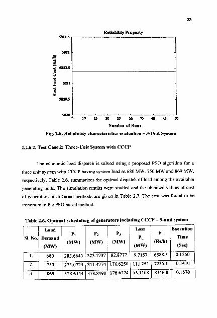
Fig. 2.5, shows the convergence characteristics of the proposed algorithm for a

load demand (PD) of 585 MW with losses neglected. Fig. 2.6. shows the reliability of

the proposed algorithm for different runs of the program. The figure shows that the

algorithm is capable of obtaining a faster convergence for the three unit thermal

system in a very few generations and the solution is consistent.

Convergenece Property 5865

Ls r,-- d = .

51190.

S I S .

110 5 LO IS 20 l5

Number of Generations

Fig. 2.5. PSO based ELD convergence characteristics -3-unit system

5 - 5 1 0 1 5 m U m 3 5 . 0 U 5 0

Nmnber of Runs

Fig. 2.6. Reliability characteristics evaluation - 3-Unit System

2.2.6.2. Test Case 2: Three-Unit System with CCCP

The economic load dispatch is solved using a proposed PSO algorithm for a

three unit system with CCCP having system load as 680 MW, 750 MW and 869 MW,

respectively. Table 2.6. summarizes the optimal dispatch of load among the available

generating units. The simulation results were studied and the obtained values of cost

of generation of different methods are given in Table 2.7. The cost was found to be

minimum in the PSO based method.

Table 2.6. Optimal scheduling of generators including CCCP - 3-unit system

Table 2.7. Solution of diierent metbods including CCCP - 3-unit system

2.2.6.3. Test Case 3: Six-Unit Thermal System

SI. No.

The third case of a six unit thermal system is solved by the PSO method and

the optimal scheduling of generators for the load demands of 700 MW and 800 MW

is tabulated in Table 2.8. The results obtained by the proposed algorithm are

compared with other evolutionary computing techniques and are given in Table2.9.

Table 2.8. Optimal scheduling of generators - 6-unit system

1821

Load Demand

(MW)

GA Method

(Rs/b)

sl.

Vc)

1.

2 .

Proposed

PSO Method

laad

I>cmand

(MW)

700

800

P,

(MW)

16.56

25

P,

(MW)

24.73

12

P,

(MW)

138.2

116

P,

(MW)

116.6

182

PI

(MW)

208.4

287

P,

(MW)

214.2

203

I;,

(Rslh)

36987

42114

h a s

PL

(MW)

18.8

26

Excrulic~n

l'lmr (Srr)

1.172

1.609

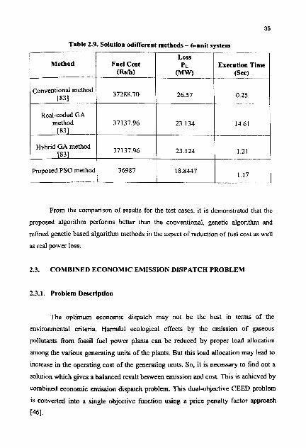
Table 2.9. Solution odiffereut methods - Cuoit system

Fuel Cost 1 Loss PI

Real-coded GA 1 t h d I 37l37: 1 23.134 14.61

. ..

Execution Time

conventional method ~331

1 proposed PSO method 1 36987 1 18.8447 1 1.17

37288.70

Hybrid GA method [831

From the comparison of results for the test cases, it is demonstrated that the

proposed algorithm performs better than the conventional, genetic algorithm and

rcfined genetic based algorithm methods in the aspect of reduction of fuel cost as well

as real power loss.

2.3. COMBINED ECONOMIC EMISSION DISPATCH PROBLEM

26.57

37137.96

2.3.1. Problem Description

0.25

The optimum economic dispatch may not be the best in terms of the

environmental criteria. Harmful ecological effects by the emission of gaseous

pollutants from fossil fuel power plants can be reduced by proper load allocation

among the various generating units of the plants. But this load allocation may lead to

increase in the operating cost of the generating units. So, it is necessary to find out a

solution which gives a balanced result between emission and cost. This is achieved by

combined economic emission dispatch problem. This dual-objective CEED problem

is converted into a single objective function using a price penalty factor approach

[461.

23.124 1.21

2.3.2. Objective Function

Optimization of generat~on cost has been fomiulatrd based on classical E1.D

with emission and line flow constraints. The deta~led problem is gluen 1161 as

follows.

where F is the optimal cost ofgenerat~on.

FC and EC are total fuel cost and emission costs of generators, respect~vely.

d represents the number of generators connected in thc network

The minimum value of the above otyect~ve funct~on has to bc found our

subject to constraints given by Eqs (2.3) and ( 2 . 5 )

The power flow equatlon of the powcr network (461

where P, and Q, are calculated real and reactive power for PQ bus i.

respectively;

P,"" and Q,"" are specified real and react~ve power for PQ bus i,

respectively;

P,.I,, and P z , , arc calculated and specified real power for PV bus m,

respectively;

I v ~ and 6 are voltage magnitudes and phase angles of different buses.

The inequality constraint on voltage of each PQ bus [46]

V- (I) S V, S V- (I)

where V,, (i) and VmX(1) are minimum and maxlmum voltage at bus I.

respective1 y

The maximum power limit on transmrssion line 1461 IS given by

where nl represents number of lines,

~f d"MVA 1s the calculated l ~ n e flow of each transmlsslon line.

~f,,"~""* is the rated llnc flow of each transmission line.

Total fuel cost of generation FC In terms of control variables generator powcrs

can be expressed [46] as follows.

where P, is the real power output of an iU' generator inMW

i represents the corresponding generator.

a , , b, ,c , are the fuel cost coefficients of generators.

The total emission release can be expressed [46] as

where a, ,p , ,y , are emission coefficients of generators

The dual-objective combined monomic emission dispatch problem is

converted into single optimization problem by introducing a price penalty factor h

[92] as follows.

Minimize 0, = FC + h x EC $/h (2.22)

subjectad to the power flow constraints of equation (2.3, 2.5, 2.17. 2.18 and 2.19).

The price penalty factor h blends the emission with fuel cog and a, is the total

operating wst in $h.

The price penalty factor h, is the ratio between the maximum fuel cost and

maximum emission of corresponding generator.

The following steps are used to find the price penalty factor for a particular

load demand:

1. Find the ratio between maximum fuel cost and maximum emission of each

generator

2. Arrange the values of price penalty factor in ascending order.

3. Add the maximum capacity of each unit (P,'"lu) one at a time. starting from the

smallest h, until Po"" > P,, .

4. At this stage, h, associated with the last unit in the process is the price penalty

factor h for the given load.

The above procedure gives the approximate value of price penalty factor

computation for the corresponding load demand. Hence a modified price penalty

factor (h,) is used to give the exact value for the particular load demand. The first two

steps of h computation remain the same for the calculation of modified price penalty

factor. Then it is calculated by interpolating the values of h, corresponding to their

load demand values.

2.3.3. Step-by-step algorithm

The step-by-step algorithm for the proposed method is explained as follows:

1. Specify the maximum and minimum limits of generation power of each

generating unit, maximum number of iterations to be performed and fuel cost

coefficient of each unit.

2. Initialize randomly the individuals of the population according to the limit of

each unit including individual dimensions, searching points, and velocities.

These initial individuals must be feasible candidate solutions that satisfy the

practical operation constraints.

3 To each chromosome of the population the dependent unit output Pd will be

calculated from the power balance equation and B-coeficient loss formula is

employed to calculate the transmission loss P i .

4. Calculate the evaluation value of each population P,, using the evaluation

equations (2.20) and (2.21).

5. Calculate the price penalty factor using the equation (2.24).

6. Compute the new evaluation function using the equation (2.22).

7. Compare each population's evaluation value with its pbest. The best

evaluation value among the pbest is denoted as gbest.

8. Modify the member velocity V of each individual P,, according to thc

equation (2.1 2).

9. Check the velocity components constraint occurring in the limits using the

conditions (2.1 3).

10. Modify the member position of each Individual P,, according to the equation

(2.14). If P,,d'"'l must satisfy the constraints, namely the generating limits.

described by (2.5). If Pgdl''" violates the constraints, then P,~"'" must be

modified towards the near margin ofthe feasible solution.

I I. If the evaluation value of each population is better than the previous pbest the

current value is set to be pbest. If the best pbest is better than the gbest the

value is set to be gbest.

12. If the number of iterations reaches the maximum then go to step 13, otherwise

go to step 3.

13. The individ-d that generates the latest gbest is the optimal generation power

of each unit.

14. After obtaining the global optimum solution, power flow is computed using

Newton-Raphson method and the calculated MVA of line flow is compared

with the rated MVA of line flow.

IS. If the line is found to be overloaded previous gbcst value is chosen as the

global optimum solution.

16. Stop

2.3.4. Simulation Results

The proposed algorithm is applied to an IEEE-30 bus system. The total system

load demand is 283.4 MW whose data has been given in Appendix-A. In the proposed

approach minimum generation cost of the generating units was obtained using PSO

based ELD in CEED environment. The line flows in the system was compared using

Newton-Raphson method. The simulation studies were carried out using a P-IV 2.4

(;Hz. 512 MB DDR RAM system in MATL.AB environment. Tahle 2.10. provides the

simulation parameters of the proposed PSO algorithm. The execution time for the

PSO based method is obtained as 79.9220 seconds. Fig. 2.7. shows the convergence

characteristics of PSO based ELD algorithm. The maximum. average and minimum

cost of generation are presented for an IEEE-30 bus system. Tahle 2.1 1. summarizes

the minimum solution obtained by particle swarm optimization based economic load

dispatch with line flow constraints for the bus system. The minimum solution includes

optimum generations, total loss. total fuel cost for IEEE-30 bus system. Table 2.12.

shows the comparison of optimal generation schedule obtained by the PSO based

method with other evolutionary techniques. The best generation of IEEE-30 bus

generating units obtained from PSO-CEED algorithm and is presented in the Fig. 2.8.

Table 2.10. Parameters used in PSO method - IEEE-30 bus system

7 Parameter

Population size

Number of iterations I

Value

50

100

W m

Wmm

Acceleration coefficients, c~,cz

0.9

0.4

2.0,2.0

rphlc 2.12. Minimum power dispatch results h? \nriou\ methods - IF:EI<-JO hu\

Table 2.1 1. E L D results obtained h? various methods - IEEE-30 bus system

Method

Nmnbsr of Censratlans

Fig. 2.7. PSO-based E L D convergence chmrncteristics - IEEE-30 hus

system

system

O\erall cost (SIh) Loss (MW)

1.u-1~~ 1x51

EP

I45l -

173.848

49 948

S A

In5l

I XX 02 .-

-17 15

14 77 --

13 40 . - - .

(;rncrnl~,r

P C I H C ~ (MW) -. -

1'1 -- P .

1 I>. ,~

1 805 4500

PTOP(IS(YJ

I'SO .. -. --

I55 6326

20 0000 .. .. .

EIb1.F

1851

I 92 05

-18.92

10 26 - -

I I o ~ o o

1 1'/ 1

21.386

l'x

10 7 0

47 0000

2q 0000 --

I 0 58

1 1 25

12 0000 -. ----

0 2770

- 12978

I,, ,

r---- PI

--- 7 2 630 - - --

--

. --- 35 0000

12 74

1 1 04

14 0') 12 000 . . - - - - -

I 0 58 9 .?YO

Gansrnror N-bsr

Fig. 2.8. Best generator settings of PSO-based <'EEL) method -1EEE-30 bus

system

I h e line l l o w s in M V A l i ~ r Ihc co lnh~ncd econonlic cmishion d~spatcl i

c<,rrc\pr,nding to the he\t generation schcd i~ lc ti)r 11.1 f ,-30 hus \?SICITI arc \h(~nti 111

I ,~hlc 2.13. I'he line5 were not ovcrloadcd u ~ t h lhc cconornic scheduling 01'

ccncrat<lrs.

'l'able 2.13. Line f lows with line flow constraints - IEEE-30 bus syslem

Line flow in M\'A Hated M V A

The computational procedure of price penalty factor for IEEE-30 bus system

is explained as follows. The ratio between the maximum fuel cost and minimum

emission of six generating units are found and arranged in ascending order.

h,= [h, hq h6b3 h~ hll

h, = [ I .7707 1.7916 2.0534 2.2198 2.33 10 2.34361

The corresponding maximum limits of generating units are given by

p,- = [30 35 40 50 80 2001

For a load of Po MW starting from the lowest h, value, the maximum capacity

of the units is added one by one (m) and when this total equals or exceeds the load. h,

associated with the last unit in the process is price penalty factor [92].

rn = [30 65 105 155 235 4351

For PD = 283.4 MW, (30+65+105+155+235+435) MW>283.4MW.

Hence price penalty factor (h) is determined as 2.3436 for IEEE-30 bus

system. Even though the price penalty factor was computed for 283.4 MW but it gives

the value up to a load demand of435 MW. So the modified price penalty factor 1461

IS computed by interpolating the values of h, for the last two units by satisfying the

corresponding load demand.

where h, is the modified price penalty factor in $/kg,

h,, is the price penalty factor associated with the last unit in $/kg.

h,2 is the price penalty factor associated with the current unit in $/kg.

P,,, is the Maximum power associated with the last unit in MW,

PmaS is the Maximum power associated with the current unit in MW

By following the above procedure, the minimum solution was obtained by the

proposed PSO method for IEEE-30 bus system as given in Table 2.14. By

incorporating modified price penalty factor approach, the total operating cost of

1624 $/h was obtained. The convergence characteristics for the PSO method are

shown in Fig. 2.9.

Table 2.14. CEED r a u b - IEEE-30 bus system

Price Emission

Penalty

Factor FC

Number orCanadonr

Fig. 2.9. PSO-based CEED convergence characteristics -

IEEE-30 bus system

PSO

2.1. ECONOMIC DISPATCH PROBLEM WITH PROHIBITED

OPERATING ZONES

2.4.1. Problem Description

2.3340

Economic dispatch is an important daily optimization task in the power system

operation. Large modem generating units with multivalve steam turbines exhibit a

large variation in the input-output characteristic functions. Thus, the practical ED

planning must perform optimal generation dispatch among the generating units to

835.5655 377.2407 1624 5.664

sat~sfy the system load demand and practical operation constraints of generators that

lnclude the ramp rate limits and the proh~bited operating zones.

2.4.2. Objective Function

The objective of ED problem IS to minlmlze the total fuel cost of power plants

subjected to the operating constraints of a power system. Generally. ~t can he

formulated with an objective function. subject to the practical operation constraints of

generator [42].

d

Minimize F, = F, (P, ) (2.25) 1-1

where F, is the total generation cost,

F,(P,) is the cost function of I ' ~ generator.

a,,b,,c, are thc cost coefficients of i I h generator.

P, is the real power generation of i I h generator,

d represents the number of generators connected in the network.

The minimum value of the above objective function has to be found out by

sat~sfying the following constraints.

Power balance Constra~nt, in which

The cost is optimized with the following power system constraint [42]

where PD is the total load of the system and

PL is the transmission power loss of the system

Ramp rate limit constraint

In ELD research, a number of studies have focused upon the economical

aspeas of the problem under the assumption that unit generation output can be

adjusted instantaneously. Even though this assumpt~on s~mplifies the problem. it does

not reflect the actual operating processes of the generating un~t . The operating range

of all on-line units is restricted by their ramp rate l~mits [SO]. Fig.2.10. shows three

situations when a unit is on-line from hour 1-1 to hour I. Fig 2.1qa) shows

that the unit is in a steady operating status. F I ~ 2.1qb) shows that the unit is in an

~ncreasing power generation status. Fig. 2.1qc) shows that the unit is in a decreasing

power generation status.

P' 'I' --

(a) @) (c)

Fig. 2.10. Three possible operating conditions of a generating unit

(i) as generation increases [42]

P, -pan S U R ,

(ii) as generation decreases [42]

P," - P, < DR,

where P, is the power generation of unit I,

P,' is the power generation ofunit i at previous hour,

UR, is the ramp rate limit of unit i as power generation increases and

DR, is the ramp rate limit of unit i as power generation decreases

The ramp rate constraints restrict the operating range of the physical lower and

upper limit to the effective lower limit P,m' and effectwe upper limit^,'"", respectively [42].

Hence the ramp rate constraint is stated [42] as

Prohibited Opaating Zone Constraint, in which references [42] have shown

the input-output performance curve for a typical thermal unit with many valve

points. These valve points generate many prohtblted zones. For a unit with

prohibited operating zones, the zones dlvlde the opcratlng region between the

minimum generation limit (P"") and the maximum generation limil (PMU).

These prohibited operating zones are due to phystcal limitations of power

plant components such as vibrations In a shatt heanng which amplified in a

certain operating region. For a prohlblted zone. the unit can only operate

above or below the zone [42].

where z is the number of prohibited zones of a unlt,

P,L,P,'> are the Lower and Upper llmlts of z proh~h~ted zones of unit i

(MW).

11 is the lower limlt of the prohibited operating zone of unit i,

ul is the upper limit of the prohibited operating zone of untt i,

d is the number of generating units,

P,"" is the effective lower limit of iCh unit with ramp rate constraint,

P,"" is the effective upper limit of iIh unit with ramp rate constraint.

The total transmission network losses is a function of unit power outputs that

can be represented using B coefficients [42]:

where P, and PJ are the real power injections at i* and j" buses,

respective1 y,

B , are the B-coefficients of transmission loss formula,

B, is the vector of same length as generators,

Boo is a constant.

2.43. Futures of Genetic Algorithms

A global optimization technique known as genetic algorithm (GA). a

probabilistic and heuristic approach is used to solve power system optimization

problems. Genetic algorithm. unlike strict mathematical methods. has the apparent

ability to adapt to nonlinearities and discontinuities commonly found in the

optimization problems. Genetic algorithms are attractive and serve as an alternative

tool for solving combinational optimization problems and they are found to hc

superior in their parallel search ability that climbs many peaks in parallel.

Genetic algorithms are adaptive heuristic search algorithms premised on the

evolutionary ideas of natural selection and genetics (41. The basic concepts of GAS

are designed to simulate processes in natural system. necessary for evolution.

specifically those that follow the principles first laid down by Charles Darwin of

survival of the fittest. As such they represent an intelligent exploitation of a random

search within a defined search space to solve a problem.

First pioneered by John Holland in 1960. Genetic algorithms have been widely

studied. experimented and applied in many fields in engineering world. Not only does

CiAs provide alternate methods for solving problems but it consistently outperforms

other traditional methods in most of the problem links. Many of the real world

problems involved in finding optimal parameters. which might prove difficult for

traditional methods are ideal for GA's 1491. They can solve problems that do not have

a precisely defined solving methods. or if they do. when following the exact solving

method would take far too much time. The genetic algorithm on the other hand, works

only with the objective function information in a search space for an optimal

parameter set.

2.43.1 Components of Genetic Algorithms

GAS are derived from a simple model of population genetics. They have the

following five components (861:

(i) String representation of the control variables

(ii) An initial population of strings.

(iii) An evaluation function that plays the role of the envimnment. rating the

strings in terms of their fitness i.e., their ability IO survive.

(iv) Genetic operators determine the composition of a new population

generated from the previous one by reproduction. crossover and mutation.

(v) Value of the parameters that the GAS use.

Since GAS are based on n a h d genetics, there exists strong analogies between

genetic algorithm and natural genetics. The strings are similar to chromosomes in

biological systems, where the chromosomes are composed of genes, which may take

any of several forms called "alleles" 1871. If the control variables are represented in

binary bits and concatenated to form a string, then it is called as binary coded GA and

if the control variables are represented in real numbers. then it is called as real coded

GA. GAS do not work with a single string but with a population of strings. which

evolves iteratively by generating new strings taking the place of their parents. GAS

treat the problem, as a black box in which the input is the strings and the output is

their fitness.

Three basic operators comprise a GA. They are reproduction, crossover and

mutation. Reproduction is the mechanism by which the most highly fit members in a

population are selected to pass on information lo the next population of members. It

effectively selects the finest of the strings in the current population to be used in

generating the next population. In this way. relevant information concerning the

fitness of a string is passed along to successive generations. It can be shown that GAS

actually allocate exponentially increasing trials to the most fit of these strings.

Crossover serves as a mechanism by which strings can exchange information.

possibly creating more highly fit swings in the process and allowing the exploration of

new regions of the search space 1871. Many types of crossovers are available like

single point crossover, multipoint crossover, uniform crossover and window

crossover. The last of the GA operators is mutation, and is generally considered as a

secondary operator. Mutation ensures that a string position will never be fixed at a

certain value for all time. Like other stochastic methods, GAS require a number of

parameters, which are population size, probability of crossover, probability of

mutation. Usually small population size, high crossover probability and low mutation

probability are recommended [88].

Tbe GA's can be distinguished h r n other optimization methods in four

different ways as follows:

(i) GA's use objective function information to guide the search, not the

derivatives or other auxiliary information.

(ii) GA's use a coding of the parameters used to calculate the objective

function in guiding the search, not the parameter themselves.

(iii) GA's search through many points in the solution space at one time. not a

single point.

(iv) GA's use probabilistic rules, not deterministic rules, in moving from one

set of solutions (a population) to the next.

The sofi computing techniques for optimization are mainly hased on GA.

Though the GA methods have been employed successfully to solve complex

optimization prohlems, recent research has identified some deficiencies in GA

performance. This degradation in efficiency is apparent in applications with highly

ep~.s/a/ic objective functions ( i .~ . . whcre the parameters being optimiied are highly

correlated) [the crossover and mutation operations cannot ensure betier fitness of

offspring because chromosomes in the population have similar suuctures and their

average fitness is high towards the end of the evolutionary process] 1891. 1901.

Moreover. the premature convergence of CiA degrades its performance and reduces its

aearch capability that leads to a higher prohahility toward obtaining a local optimum

1x91.

2.4.4. CA and PSO Combined Hybrid Method

2.4.4.1. Deseription of the proposed method

In this work, a hybrid genetic-PSO search (hybrid GA-PSO) algorithm is

proposed d i c h utilizes Genetic algorithm to explore the high performance region in

solution space and PSO algorithm to exploit the solution space for locating the

optimal solution. Thus, the GA guides PSO for better performance in the complex

solution space. In this work, the constrained economic dispatch problem is solved by

the integrated GA-PSO algorithm and a high quality solution is obtained for a

practical power system opemtion. The GA-PSO algorithm is utilized to determine the

optimal generation power of each unit that was usad in operation at the spacific

period, thus minimizing the total generation wst.

2.4.4.2. Evaluation Function

The evaluation function f (it is called fitness in GA) must be defined for

evaluating the fitness of each individual in the population. For emphasizing the best

chromosome and faster convergence of the iteration process, the evaluation value is

normalized in the range between 0 and 1. The evaluation function f is given in

equation (2.34) which is the reciprocal of the summation of generation cost function

F,,,, and power balance constraint P*L 1421.

1 f=-- F,,,, + p,,

where

FC", = I + abs (F~." - F,"," )

F,, and F,,,, are the maximum and minimum generation cost among h e

~ndividuals in the initial population.

2.4.4.3. Application of GA-PSO Algorithm

The sequential steps of the proposed hybrid GA-PSO algorithm are shown as

below:

1. Initialize randomly the individuals of the population according to the limit of

each unit including individual dimensions, searching points, and velocities.

These initial individuals must be feasible candidate solutions that satisfy the

operation constraints.

2. To each chromosome of the population the dependent unit output Pd will be

calculated fmm the power balance equation and B coefficient matrix.

3. Calculate the evaluation value of each individual P,, in the population using

the evaluation function f given by equation (2.34).

4. Compare each individual's evaluation value with its pbest. The best evaluation

value among the pbest's is denoted as gbest.

5. Modify the member velocity V of each individual PK according to the equation

(2.1 2).

6. Check the velocity components constraint occurring in the limits using the

conditions (2.13).

7. Modify the member position of each individual P,, using (2.14). if P,~"*"

violates the constraints, then \d"*" must be modified toward the near margin

of the feasible solution.

8. Apply the genetic operators selection. crossover and mutation to the above

population and generate offspring. Now compare the parents and offspring to

select the fittest chromosomes for the next step.

9. If the evaluation value of each individual is better than previous pbest. the

current value is set to be pbest. If the best pbest is better than gbest. the value

is set to be gbest.

10. If the number of iterations reaches the maximum. then go to step 11.

Otherwise. go to step 2.

11. The individual that generates the latest gbest is the optimal generation power

of each unit with the minimum total generation cost.

2.4.5. Simulation Results

To verify the feasibility of the proposed hybrid algorithm, the 6-, 15- and 40-

unit systems are tested. The ramp rate limits and prohibited operating zones of the

units were taken into consideration. The proposed hybrid GA-PSO algorithm is

compared with the GA and the PSO methods. Under each sample system, 50 trials

were performed using the same evaluation function with the proposed algorithm. This

gives a fair comparison of the proposed GA-PSO method with the aspects of

Computational efficiency and a qualitative solution. An optimal range of inertia

weight and acceleration factors for the PSO algorithm is estimated for 6, 15- and 40-

unit test cases in this research. On comparison of the results. it has been demonstrated

that the proposed algorithm is capable of obtaining higher quality of solution

efficiently for economic dispatch problem covering prohibited operating zones.

AAer many experiments. the following parameters have been selected for the

proposed hybrid GA-PSO algorithm.

Table 2.15. Parameters used in GA-PSO method - Cunit, 15-unit, 40-unit

systems

Parameter

Generations

Wmm

2.4.5.1. Six-Unit System

Value

100

0.9

Wmsn

Acceleration coefticients ~ 1 . ~ 2

Crossover probability

I-. Mutation probability

The system contains six thermal units. 26 buses and 46 transmission lines and

the data were taken from [42]. The cost coeficients, generating unit capacity limits.

ramp rate. prohibited operating zones and loss coeflicients are provided in

Appendix-B.

Po~ulation size I 50

0.4

2.0.2.0

0.55

0.01

The load demand is 1263 MW. To simulate this system, each individual P, contains

six generator power outputs. Since one unit is considered as a dependent unit. each

individual in the population contains five generator power outputs. The dimension of

the population is equal to 50x5. Table 2.16 shows the best solution obtained by the

proposed algorithm and its comparison with the GA and PSO methods. Table 2.1 7

shows the comparison of average generation cost and average CPU time of different

methods.

Table 2.16. Optimal generator dispatch solution by various methods - bunit

Table 2.17. Comparison of solution quality - 6-unit system

system

Output Power (MW)

The comparison of the performance of proposed algorithm with other methods

demonstrates that the solution quality and computation efficiency is good for the

hybrid algorithm.

GA Method

(421

Average

CPll Time

(see)

41.58

14.89

12.72

Method

GA method [42]

PSO method

[421

Hybrid GA-PSO

1 method

PSO Method

1421

Generation Cost ( S h )

Hybrid

CA-PSO

Method

--

Minimum

15,459

15,450

--

15.444

Maximum

15,524

15.492

15,488

Average

15.469 -

15.454

15.45 1

2.4.5.2. Fifteen-Unit System

This system contains 15 thermal generating units whose characteristics and

transmission loss (B loss) coefficients are Inken from [42] and are provided in

Appendix<. The total power demand of the system is 2630 MW. To simulate this

system, each individual P, contains 15 generator power outputs. Since one unit is

considered as a dependent unit, each individual in the population contains 14

generator power outputs. The dimension of the population is equal to 50x 14. The

simulation results are shown in Tables 2.18 and 2.19.

Parameter GA Method 142) PSO Method 1421 Hybrid CA-PSO

Method PI 415.3108 439.1 162 436.8482

Table 2.18. Optimal generator dispatch solution by various methods - IS-unit system

2668.4 2662.4 2661.75

! power loss (MW) 38.2782 32.4306 3 1.752

r Power ou tpu t (MW)

m i o n

cost ( S h ) 33.1 13 32,858 32.724

Table 2.19. Comparison of solution quality - 1Sunit system

For a power demand of 2630 MW, the total transmlsslon losses are 31.75 MW

the optimal dispatch is obtained by the proposed algorithm. Since the total power

output from all the 15 units are 2661.75 MW. the power balance equatron is exactly

sat~sfied. The total generation cost as well the power losses are less for Ihe proposed

algorithm compared with GA and PSO methods By comparing the results obtained

hy various methods, it is found that the proposed algorithm is capable of providing

Method

GA method

[421

PSO method

1421

Hybnd GA-PSO

method

optimal solution.

2.4.5.3. Forty-Unit System

The system consists of 40 units ~n the realistic Taipower system which is a

large-scale and mixed-generating system with coal-fired, oil-fired, gas-fired, diesel

and combined cycle cogeneration units [50]. The cost coeficients of Taipower 40-

unit are shown in Appendix-D. The system load demand is 8550 MW. Since one unit

1s considered as a dependent unit, each individual in the population contains 39

generating unlt outputs. The dimension of the population is 50 x 39. The simulation

results and a comparison of performance are given in Tables 2.20 and 2.2 1.

Average

execution

time (Sec)

49 31

26 59

- - - Generation Cost (yb)

Minimum

33,113

.

Maximum

32.724

- -.

Average

77,188

-

72,984

73,039

-

32,858

27 52

--

33.337

- -

33,331

.- - -- -

13.228

. --

Table 2.20. T a t results of the proposed approacb- 40-unit system

- -J I. .I

CA Method I M , r o d 1 Output Power (MW) 1 ,421

Table 2.21. Comparison of solution quality - 40-unit system

Total power output (MW)

Power loss (MW)

Total generation cost ($/h)

GA method 135.070 1 137,980 1 137.760 1 81.80 1 1421

Method

I GA-PSO 130,255

8636.582

86.58

130,255

8641.08

89.76

135,070

( method 1 1 I I I

8637.26

87.24

130.380

Solution Quality

Average

CPU Time

(a=)

Generation Cost (Sth)

The developed software package has k e n executed 50 different runs Ibr the

proposed hybrid GA-PSO algorithm and the results are given in Tables 2.16 to 2.20.

From the comparison of results shown in the tables. it is evident that the proposed

hybrid GA-PSO algorithm for three systems has obtained low generation cost in

comparison to the PSO and GA methods. Fig. 2.1 1 shows the plot of convergence of

best solution obtained by the proposed algorithm for a 15-unit system. There is an

indication of a better quality of solution obtained by the proposed method when

compared to other methods.

Minimum Maximum Average

Fig. 2.1 1 (;A-IDSO contergence charncteristicc - 15-unit r?rtem

l.rom the cornp;lrlson 01' l ahler 2 17. 2 1') and 2.21. II can he li>und th;~t the

p~opo\ed h>brid ( ; .A- I30 ha\ Icswr a\eragc e\ccution time compred with (;A illid

1'50 nictliods. I lence. the cc~niputation ~. f l ic icno of' the proposed algorithm I\

ruccesslull! dcmonbtrated. Prom the ah~be \tud! ~t IS fi~und that. even though

c\ccution time li)r one iteration i a more hecaube o f the presence o f CiA operators.

crosso\.er and mutation. the identilication of'the high perl'bnnance region and locating

the optimal solution is pc>ssihle mithin less numher 01. ~terations tlerse it finds the

oplirnal solution within lesser average euccutlcm time.

2.5. CONCLUSION

This work adapts the particle swarm optimization algorithm and genetic

approach based particle swarm optimization algorithm to different types of economic

dispatch problems. The test results for the lEEE and the various test systems bring out

the advantage of the proposed method. The convergence abilities of the PSO method

are better than the classical evolutionary programming method. The PSO method

converges to the global or near-global p i n t , irrespective of the shape of the cost

function. for example, discontinuities in the cost functions. The better computation

efficiency and convergence property of the proposed PSO approach shows that it can

he applied to a wide range of optimization problems.