chapter 4shodhganga.inflibnet.ac.in/bitstream/10603/42092/14/14... · 2018-07-03 · 49 chapter 4...

49

CHAPTER 4

THE EFFECT OF CME ON THE TERRESTRIAL ATMOSPHERE

4.1 Introduction

Investigation of the effects of solar and interplanetary (hemispheric) events on near -Earth

space is one of the most important components of solar–terrestrial physics. In spite of the

large amount of experimental and theoretical data that has been accumulated, the prediction of

effects of the space weather faces serious difficulties. Although it has been appreciated for

some time that solar wind disturbances drive major geomagnetic activity, there is now a better

understanding of the solar causes of these disturbances. “The identification of Coronal Mass

Ejections in the sun as the primary source of the most geo effective disturbances has given

new impetus and inspiration to the space weather forecasting” (Luhmann, 1997). Only after

the advent of the coronagraphs on board the Solar and Heliosphe ric Observatory (SOHO)

mission (Domingo et al. 1995) the connection to Coronal Mass Ejections near the sun became

evident, especially those affecting earth‟s space environment.

Coronal mass ejection is a huge outbur st of solar mass into the interplanetary space.

Mostly Coronal Mass Ejections are associated with solar flares, but such a causal relationship

has not yet been established fully. Mostly Coronal Mass Ejections originate from

magnetically active region in the solar disk and the process of magnetic reconnection results

in the emission of huge amount of matter and electromagnetic radiation into space. Magnetic

reconnection is the process wherein two oppositely directed magnetic fields merge

50

Chapter4 The Effect of CME on the Terrestrial Atmosphere

and an associated rearrangement occurs. The energy stored in the earlier oppositely aligned

field lines is emitted out as intense electromagnetic waves and a portion of the sun‟s magnetic

field which is in the form of closely spaced loops may become totally unconnected forming

helical loops. These loops along with the material they contain expand violently to the outer

space forming the coronal mass ejections. If the Coronal Mass Ejections are directed towards

earth, then their influence on the earth‟s magnetic field will be tremendous. The Coronal Mass

Ejection associated particles like protons and electrons, whic h are carried by the solar wind,

enter into the earth‟s magnetosphere thereby setting up current systems and modifying the

ambient electric fields of the earth leading to modification of the existing various structures.

This phenomenon is called the geomagnetic storm. The solar energetic particles having

energies of the order of keV to MeV cause strong auroras in the polar region which is caused

due to the particle entry into the earth through polar cusps. Once CME is ejected by the sun,

ideally it takes one to five days to reach the earth depending on the velocity of streaming

particles. If the solar wind velocity is larger than CME velocity, it accelerates the CME

particles and if CME velocity is higher than solar wind velocity it is decelerated. Very fast

CMEs can drive a shock wave if their velocities are faster than the sonic speed.

Large CME driven interplanetary disturbances are usually preceded by strong shocks that are

effective accelerators of particles and sources of radio emission. The enhanced S EP

production at stronger or faster shocks driven by the fast CMEs, can exceed the Alfven and

flow speeds of the solar wind (Zank et al. , 2000). Early studies established that there is a

rough correlation between the logs of the CME speed and the logs of the SEP intensities. The

outermost structure of fast CMEs is an MHD shock, which will first interact with the

preceding CME. The shock has to pass through the heterogeneous multi thermal plasma

51

Chapter4 The Effect of CME on the Terrestrial A tmosphere

(core, cavity, and frontal of the preceding CMEs). Thus, the shock has to accelerate the SEPs

from the solar wind "contaminated" by the preceding CMEs, rather than from the quiet solar

wind. The interaction rather than the speed of the preceding CMEs seems to be important for

the SEP production (Gopalswamy et al. , 2002). Gopalswamy (2002) concluded that the

efficiency of the CME-driven shocks is enhanced as they propagate through the preceding

CMEs and that they accelerate SEPs from the material of the preceding CMEs rather than

from the quiet solar wind. Thus the discovery of CMEs and their roles in driving

interplanetary shocks changed the focus of our understanding of SEP sources.

The relation between solar energetic protons and coronal mass ejections was studied

more directly by Kahler et al. (1978) who suggested that CMEs are required for proton events.

Solar proton events (SPE), also known as polar cap absorption (PCA) events in the history of

radio physics, begin as emission of electrons and ions from the surface of the Sun. The ions

are mostly protons (≈ 90%) but heavier particles are also emitted, the relative abundances

being similar to those in the solar corona. For the most energetic coronal mass ejections

(CME), particle energies can be up to MeV or even GeV level, thus far exceeding the normal

solar wind values,

The acceleration of emitted particles is driven by processes related to the solar flare

accompanying the CME, and/or by solar wind shock fronts (Cane and Erickson, 2003).Even

particles having GeV energies are guided by the interplanetary magnetic field (IMF) over the

sun-earth distance. Therefore, the emitted particles will follow the spiral field lines of IMF,

and the location of the CME on the solar surface will determine wheth er or not the released

particles will hit the earth‟s magnetosphere. Also, the guidance of IMF results in some

additional time delay between the CME and the arrival of particles on earth. Typically, a

delay of several hours is observed. Particles having different energies have different Larmor

radii, and the particles with lower energies are more sensitive to the form of IMF. As a result,

the bulk velocity of the particle “cloud” is much less than that of individual particles,

e.g. ∼ 1 keV for protons.

52


which can be used to explain the duration of near-earth effects, typically of the order of days,

and the isotropic angular distribution of the particles near the earth(Verronen et al., 2002).

In order to reach the atmosphere of earth, the particles have to interact with the

magnetosphere, at various high energies. The magnetosphere trajectories of high -energy

particles can be calculated using the Störmer theory (Störmer, 1950). According to the Störmer

theory, every geomagnetic latitude has a cut-off limit which the rigidity of an incoming

particle (defined as momentum per charge) must exceed for it to reach that particular location.

Penetration to lower latitudes requires higher rigidities, and certain latitude is a ffected by

particles having rigidity equal to, or higher than the corresponding cutoff. The cut - off rigidity

varies spatially and also with time, being dependent on the IMF as well as on the earth‟s

internal magnetic field, and on timescales from minutes to years. The magnetic storms, for

example, tend to compress the magnetosphere and lower the cutoff rigidity for given latitude.

As a consequence of geomagnetic cutoff, the particles are able to affect atmosphere above

certain magnetic latitude, covering the polar cap regions in both hemisphere. Typically

latitudes above about 60◦ are affected more or less uniformly, although the effects have

sometimes been observed near the geomagnetic poles first, and later throughout the polar cap

(Buonsanto, 1999).

Ionospheric storms are closely associated with geomagnetic storms. The disturb ances,

when affecting the ionosphere are known as ionospheric storms; tend to generate large

disturbances in ionospheric density distribution, total electron content, and the ionospheric

current system. Ionospheric storms have important terrestrial consequences such as disrupting

satellite communications and interrupting the flow of electrical energy over power grids.

Buonosanto (1999) has indicated that ionospheric storms represent an extreme form of space

weather with im portant effects on ground and space-based technological systems. The

ionosphere is an open system that strongly couples with the magnetosphere and thermosphere.

53


Various photochemical, chemical reactions, dynamical and electro dynamical processes in the

system exchange and transport mass, momentum and energy in a complex manner (Rees,

1989). The SPEs provide a direct connection between the sun and the earth‟s middle

atmosphere. Ionospheric disturbances during solar proton events have been observed almost

solely by radio techniques, especially by riometers and incoherent scatter radars.

The earth‟s ionosphere, responds markedly to varying solar and magnetospheric

energy inputs. During geomagnetic storms, the disturbed solar wind com presses the earth‟s

magnetosphere and intense electric fields are mapped along geomagnetic field lines to the

high latitude ionosphere. At times these penetrate to low latitudes, and at high latitudes they

produce a rapid convection of plasma which also drives the neutral winds via collisions. At

the same time energetic particles precipitate to the lower thermosphere and below, expanding

to the auroral zone, and increasing ionospheric conductivities. Intense electric currents couple

the high latitude ionosphere with the magnetosphere and the enhanced energy input causes

considerable heating of the ionized and neutral gases. The resulting uneven expansion of the

thermosphere produces pressure gradients which drive strong neutral winds. The disturbed

thermospheric circulation alters the neutral composition and moves the plasma up and down

magnetic field lines, changing rates of production and recombination of the ionized species.

At the same time the disturbed neutral winds produce polarized electric f ields by a dynamo

effect, as they collide with the plasma in the presence of the earth‟s magnetic field. These

electric fields in turn affect the neutral and plasma alike, illustrating that the ionized and

neutral species in the upper atmosphere are closely coupled, so it is not possible to attain a

physical understanding of geomagnetic storm effects on ionospheric electron density without

considering the effects on the neutral thermosphere (Buonsanto, 1999; Gopalaswamy,

2011).This chapter however concerns with the effect of CMEs and geomagnetic storms in the

terrestrial ionosphere over equatorial la titudes. The ionospheric response to solar flares has

been widely studied with multiple instruments since the 1960s.

54


This work presented in the following sections investigates the effects of CMEs on the

equatorial ionosphere through analysis of the correlation between CME parameters (linear

speed and angular width) with ionospher ic parameters (h‟F i.e. ionospheric base height as

inferred from ground based ionosonde measurements and electron density). The correlation of

CME parameters (linear speed and angular width) with the solar wind speed is also discussed.

4.2 Data and Methodology

The severest of geomagnetic storms and the largest of solar energetic particle (SEP)

events have been shown to be caused by energetic CMEs. The October – November 2003

period produced a large number of energetic CMEs, two of which were of historica l

importance. So study concentrated on the effect of CME parameters (linear speed and angular

width) observed by the LASCO coronagraph on the Solar and Heliospheric Observatory

(SOHO) during the months of October and November 2003 with the F region equato rial

ionospheric parameters.

These equatorial F-region ionospheric parameters were obtained from the ionospheric

measurements done using ground based ionosonde located at Thiruvananthapuram, a dip

equatorial station in India. The rationale for using the ionosonde data into the present thesis is

the following:

The terrestrial ionosphere is the direct outcome of the interaction of incoming solar

radiation with the various neutral species present in earth‟s upper atmosphere. These neutral

species get ionized as an outcome of this interaction and lead to the formation of ionosphere.

The distribution of ionosphere with altitude, latitude and longitude depends not only on the

intensity of the solar radiation and abundance of neutral constituents, but also on the

orientation of the geomagnetic field configuration. Typically, the altitudinal distribution of

ionospheric plasma exhibits the presence of two layers namely E -region and F-region, the

former lying in the ~80-140km altitude region while the latter above it. The ionospheric

altitudes and corresponding densities are obtained through the ionosonde measurements. In

making these measurements, radio waves in a range of frequencies are sequentially

55

transmitted vertically up from ground who‟s reflected echoes from ionosphere are received

after a time delay. The time delay gives ionospheric altitude and frequency of the wave

electron density at that altitude. The base height of the F -region is typically reffered to as h‟F.

These ionosonde measurements of the equatorial ionosphere are being made systematically

from Trivandrum. In view of the above, the terrestrial ionosphere is known to respond

immediately to the sudden radiation increase during solar flares manifesting as enhancement

in the overall ionization. As the CMEs are usually followed by the onset of geomagnetic

storms, the ionosphere responds to CMEs therefore after a time delay.

In this context , the ionospheric F -region height (h‟F) and electron density for the

same period were obtained from the ground-based ionosonde at Trivandrum, a dip equatorial

station in India, and solar wind speed data (hourly averages) from SOHO CELIAS Proton

Monitor. For comparison June (northern solstice), September (southward equinoxes) &

October 2004 data were also used for analysis.

The most familiar measure of dependence between two quantities is the "Pearson's

correlation coefficient”. CMEs typically reach Earth one to five days after leaving the sun. So

correlation coefficients were calculated at different time delays ranging from 3 to 96 hours

with the following CME parameters (linear speed and angular width) against ionospheric

parameters (h‟F, Electron density) and solar wind speed.

4.3 CME Link to Severe Geomagnetic Storms

It has already been established that there exists a good relationship between monthly averaged

maximum CME speeds and sunspot numbers, Ap and Dst indices (correlation coefficients are

0.76, 0.68, -0.53 respectively) (Gopalswamy, 2011). Statistical studies have shown that the

severest of geomagnetic storms (Dst < -150 nT) are always caused by CMEs. The CME link

to the geomagnetic storms is evident from the empirical relationship between Dst and the

product of Bs (nT) and the speed V (km/s) of the ICME structure (Gopalswamy, 2011).

Dst = - 0:01VBs – 32

56


CMEs and associated shocks arrive on earth as magnetic clouds. It was observed that

magnetic clouds and their shocks have large effects on magnetosphere activity, and they are

one of the main causes of intense geomagnetic storms (Echer et al., 2005). CME- CME

interactions are expected to be a frequent phenomenon in the Sun-Earth space during solar

maximum. The typical transit time of CMEs from the SUN to 1 AU is a few days, much

longer than the time within which multiple CMEs occur at solar maxim um(Ying et al., 2013).

The solar events of October and November 2003 were extraordinary, with the largest so lar

flare ever recorded, solar wind speeds at earth approaching 2000km/s. Twelve X - Class flares

were observed from 19 October to 4 November from 90 0E to 830 W on the solar surface

(Richardson et al., 2005; Malandraki et al., 2005).

4.4 Observed Ionospheric Variability

October-November 2003

Figure 4.1 shows the time variations of the geomagnetic indices such as Solar wind speed,

Dst, and F10.7 solar flux for various months considered in this investigation during 2003 and

2004.

57


Figure 4.1 shows the variations of solar wind velocity (top panels), Dst (middile panels) and F10.7cm solar flux

(bottom panels ) for different months during the year 2003 and 2004. The label on X -axis indicates the

period/months

As can be seen from the Dst variability, the -100nT which continued with a slow recovery till

October 28 only to mark the beginning of a great storm through a sudden and significant

decrease to about -400nT in Dst around October 30-31.

Figure 4.2 presents the variability of ionospheric F -region base height (Panels b and c), the

color scale indicating altitude in kilometers, and the peak electron density (Panels a and d)

from October to November 2003, the color scale indicating the frequency corresponding to

peak ionospheric density of F-region.

58


It can be seen very clearly that the ionospheric density has undergone an overall

Figure 4.2: The figure in panels a and d depicts the variability of peak electron density of Ionospheric F -region

for months November and October 2003 respectively. The panels b and c show the ionospheric base height

variations for November and October 2003 respectively. The white patches indicate no data

enhancement, especially in the afternoon hours, beyond October 13 which persisted till

November 10. However, the density enhanced once again beyond November 20. While the

corresponding base height changes are observed to be small during the noon hours, there

appears to be significant day-to-day changes in them in the post evening hours around 20:00

hrs. Figure 4.1 shows the time variations of the geomagnetic indices such as Solar wind speed,

Dst, and F10.7 solar flux during the June, September and October months of 2004. As can be

seen from the Dst variability, the ring current variability had been moderate (around -20-

30nT) throughout with no major decreases in it indicating the onset of geomagnetic storm.

59


September - October 2004

This indirectly indicates that the solar wind conditions had not changed very dramatically

during the above mentioned period. The prevailing ionospheric variability also ref lects this

aspect of prevailing quiet space weather conditions.

Figure 4.3: The figure in panels a, f and e depicts the variability of peak electron density of Ionospheric F -region

for months October, September and June 2004 respectively. The color scale represents frequency corresponding

to peak F-region ionospheric density. The panels b, c and d show the ionospheric base height variations for

October, September and June 2004 respectively. The color scales here represent the base height in kilometer of

F-region.The white patches indicate no data

60


Figure 4.3 depicts the variability of ionospheric electron density (Panels a, f, e) and base

height for (Panels b, c, d) for the June, September and October months of year 2004. It can be

seen very clearly that the ionospheric density on the whole are smaller than that observed

during Oct-Nov 2003. An enhancement is seen on a day-to-day basis in the morning and

evening hours with a minimum around noon. The corresponding base height changes are

observed to be small on the whole during the noon hours. However, as seen during Oct -Nov

2003 period, there appears to be significant day-to-day changes in them in the post evening

hours around 20:00 hrs during September-October while an absence of such a height change

during month of June is quite conspicuous.

It is clear from the comparison of ionospheric variability during 2003 and 2004 that during the

latter year the observed electron density changes are primarily governed by the large scale

process called Equatorial Ionization Anomaly (EIA) wherein the equatorial F -region

ionospheric density exhibits enhancement in the morning and evening hours with a minima

during noon (Rishbeth, 2000). The magnetospheric influences are not observed in the response

of the ionosphere. However, during the former year, the EIA appeared to have been

influenced by the ongoing magnetospheric/geomagnetic activity. Since, the geomagnetic

perturbations as inferred through the Dst had their origin in the activity on the sun i. e. the

CMEs from the sun, it was expected that the CMEs would have a bearing on the ionospheric

variations during the year 2003 which would appear as a correlation between parameters

representing CME and the ionosphere. As is known, the geomagnetic storms have a delayed

effect in the equatorial ionosphere; a time delayed correlation analysis was performed using

CME linear speed & angular width and base height of F -region of ionosphere and electron

density. It is observed that the inferred correlation coefficient varies significantly with time

delays. Table-1 to 4 summarizes the observed time-delays and the correlation coefficients for

various months used in this study. The variations of the inferred correlations with various time

delays are presented and discussed in the following sections. The inferred time delays would

indicate the time taken by the terrestrial ionosphere-magnetosphere system to respond to the

CME forcing so as to reflect in the electron densities through changes in the ionospheric

processes.

61


4.5 Correlation of CME linear speed with Ionospheric height and Electron density

Coronal mass ejections reach velocities between 20km /s to 3200 km/s with an

average speed of 399 km/s, based on SOHO/LASCO measurements between 1996 and

2008. W ith following table we can determine how long the CME will take to travel from

the sun to earth providing it does not slow down along the way.

Table 4.1: Travel time from the sun to earth for CMEs with different velocity

CME speed (km/s) Travel time (hours)

500 83.33

1000 41.67

1500 27.78

2000 20.83

2200 18.94

Gopalswamy et al. (2005b) studied the violent solar eruptions of 2003 October and

November, invoking fast CMEs, X-class solar flares, interplanetary shocks, intense

geomagnetic storms, and SEPs. These violent solar eruptions of October/ November 2003

period can be regarded as extreme events in terms of their origin as well as their

heliospheric consequences. The two earth-directed full halo CMEs produced intense

geomagnetic storm (Dst index of -363 and -401 nT for the 28 and 29 october CMEs,

respectively. Two of the halo CMEs resulted in shocks that a rrived at earth in <24 hrs.

Bhatt et a l. (2013) investigated the spectral behavior (hardness parameter β) of an SEP

event and its relation with the dynamics of the associated CME and arrived at a power-law

with a correlation coefficient of ~0.96. Tripathi et al. (2013) made a statistical study on the

evolution of solar proton events simultaneously with the dynamics of associated CMEs

and found the linear relationship between the solar proton spectral index and initial CME

velocity with fairly good correlation coefficiel (0.71). So a time delayed correlation is

62

Chapter4 The Effect of CME on the Terrestrial Atmospher

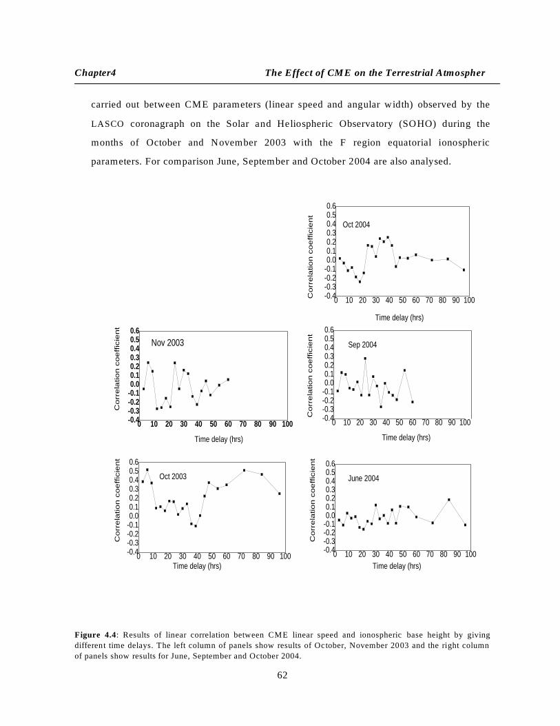
carried out between CME parameters (linear speed and angular width) observed by the

LASCO coronagraph on the Solar and Heliospheric Observatory (SOHO) during the

months of October and November 2003 with the F region equatorial ionospheric

parameters. For comparison June, September and October 2004 are also analysed.

0 10 20 30 40 50 60 70 80 90 100-0.4-0.3-0.2-0.10.00.10.20.30.40.50.6

0 10 20 30 40 50 60 70 80 90 100-0.4-0.3-0.2-0.10.00.10.20.30.40.50.6

0 10 20 30 40 50 60 70 80 90 100-0.4-0.3-0.2-0.10.00.10.20.30.40.50.6

0 10 20 30 40 50 60 70 80 90 100-0.4-0.3-0.2-0.10.00.10.20.30.40.50.6

0 10 20 30 40 50 60 70 80 90 100-0.4-0.3-0.2-0.10.00.10.20.30.40.50.6

Co

rre

latio

n c

oe

ffic

ien

t

June 2004

Time delay (hrs)

Time delay (hrs)

Co

rre

latio

n c

oe

ffic

ien

t

Sep 2004

Co

rre

latio

n c

oe

ffic

ien

t

Oct 2004

Time delay (hrs)

Co

rre

latio

n c

oe

ffic

ien

t

Time delay (hrs)

Oct 2003

Time delay (hrs)

Co

rre

latio

n c

oe

ffic

ien

t

Nov 2003

Figure 4.4: Results of linear correlation between CME linear speed and ionospheric base height by giving

different time delays. The left column of panels show results of October, November 2003 and the right column

of panels show results for June, September and October 2004.

63


Fig.4.4 shows the change in correlation coefficient between the CME linear speed and

ionospheric base height for varying time delays for five months. Table 4.2 summarizes the

observed time-delays and the correlation coefficients for various months used in this study.

The highest correlation coefficient obtained is 0.6 for a time-delay of about ~8 hrs for

October 2003. During the m onth of October 2003, most of the CMEs are fast with an average

speed of 749 km/s. The relation between the SEP event a nd the dynamics of the CME are

considered as responsible for the greater correlation in October 2003. Though the average

speed of CME is 841 km/s, the overall proton flux was substantially small during the Solar

Proton Event on November 3. In June, September and October 2004 the average speed of

CME decreased and no Solar Proton Events were recorded.

Table 4.2 : Correlation analysis between CME linear speed and Ionospheric height

Month & year Maximumcorrelation coefficient Average CME

Speed(km/S)

SPE Proton

Flux

(pfu>10MeV)

October 2003 0.5971 for ~ 8 & 72 hrs 713 29500

November 2003 0.2485 for ~ 8 & 24 hrs 841 1570

June 2004 0.1886 for ~ 85 hrs 425 Nil

September 2004 0.2805 for ~ 24 hrs 463 273

October 2004 0.2543 for ~ 42 hrs 305 Nil

64


0 10 20 30 40 50 60 70 80 90 100-0.4

-0.3

-0.2

-0.1

0.0

0.1

0.2

0.3

0.4

0.5

0 10 20 30 40 50 60 70 80 90 100-0.4-0.3-0.2-0.10.00.10.20.30.40.5

0 10 20 30 40 50 60 70 80 90 100-0.4

-0.3

-0.2

-0.1

0.0

0.1

0.2

0.3

0.4

0.5

0 10 20 30 40 50 60 70 80 90 100-0.4-0.3-0.2-0.10.00.10.20.30.40.5

0 10 20 30 40 50 60 70 80 90 100-0.4

-0.3

-0.2

-0.1

0.0

0.1

0.2

0.3

0.4

0.5

Co

rre

latio

n c

oe

ffic

ien

t

Sep 2004

Co

rre

latio

n c

oe

ffic

ien

t

Time delay (hrs)

June 2004

Oct 2004

Time delay (hrs)

Time delay (hrs) Time delay (hrs)

Co

rre

latio

n c

oe

ffic

ien

t

Co

rre

latio

n c

oe

ffic

ien

tC

orr

ela

tio

n c

oe

ffic

ien

t

Time delay (hrs)

Oct 2003

Nov 2003

Figure 4.5: Results of linear correlation between CME linear speed and electron density by giving different time

delays. The left column of panels show results of October, November 2003 and the right column of panels show

results for June,September and October 2004.

65


Figure 4.5 depicts the variation of observed correlations between CME linear speed and

electron density for different months. The observed correlations have been found to be lying

in the range -.2 to .3. These correlations are found to be insignificant.

4.6 Correlation of CME angular width with ionospheric height and Electron density

One of the basic requirem ents for CMEs to produce a geomagnetic storm is that they should

hit and interact with earth‟s magnetosphere. Statistical studies have shown that CMEs

generally propagate radially above the source regions. As a consequence, the CMEs need to

originate close to the centre of the solar disk in order to arrive on earth (Gopalswamy

2011).The width of CMEs causing geomagnetic storms typically exceed 600. So the solar

sources need to be located within a central meridian distance (CMD) ~ 300. When the CME

originates beyond ±300

meridian, only a small section of the CME might arrive on earth or

none at all, depending on the angular extent of the CMEs. Thus the CME angular width also

contributes a major role. In the present study, the time-delayed correlation analysis between

CME angular width and ionospheric height has also been carried out. Figure 6 shows the

inferred correlations and corresponding time-delays for different months.

Table 4.3 : Correlation analysis between CME linear speed and Electron density

Month & year maximum correlation coefficient

October 2003 0.1520 for ~ 42 hrs

November 2003 0.2867 for ~ 22 hrs

June 2004 0.2853 for ~ 72 hrs

September 2003 0.2946 for ~ 32 hrs


66


0 10 20 30 40 50 60 70 80 90 100-0.4-0.3-0.2-0.10.00.10.20.30.40.50.6

0 10 20 30 40 50 60-0.4-0.3-0.2-0.10.00.10.20.30.40.50.6

0 10 20 30 40 50 60 70 80 90 100-0.4-0.3-0.2-0.10.00.10.20.30.40.50.6

0 10 20 30 40 50 60 70 80 90 100-0.4-0.3-0.2-0.10.00.10.20.30.40.50.6

0 10 20 30 40 50 60 70 80 90 100-0.4-0.3-0.2-0.10.00.10.20.30.40.50.6

June 2004

sep 2004

Time delay (hrs) Time delay (hrs)

Time delay (hrs)

Time delay (hrs)

Oct 2004

Time delay (hrs)

Oct 2003

Co

rre

latio

n c

oe

ffic

ien

tC

orre

latio

n c

oe

ffic

ien

t

Co

rre

latio

n c

oe

ffic

ien

tC

orre

latio

n c

oe

ffic

ien

tC

orre

latio

n c

oe

ffic

ien

tNov 2003

Figure 4.6: Results of linear correlation between CME angular width and ionospheric base height by giving

different time delays. The left column of panels show results of October, November 2003 and the right column

of panels show results for June, September and October 2004.

67


0 10 20 30 40 50 60 70 80 90 100

-0.2

-0.1

0.0

0.1

0.2

0.3

0.4

0 10 20 30 40 50 60 70 80 90 100-0.3

-0.2

-0.1

0.0

0.1

0.2

0.3

0.4

0 10 20 30 40 50 60 70 80 90 100-0.4

-0.3

-0.2

-0.1

0.0

0.1

0.2

0.3

0.4

0 10 20 30 40 50 60 70 80 90 100-0.4

-0.3

-0.2

-0.1

0.0

0.1

0.2

0.3

0.4

0.5

0 10 20 30 40 50 60 70 80 90 100-0.4-0.3-0.2

-0.10.00.10.2

0.30.40.5

Co

rre

latio

n c

oe

ffic

ien

t

Time delay (hrs)

June 2004

Co

rre

latio

n c

oe

ffic

ien

t

Time delay (hrs)

Sep 2004

Co

rre

latio

n c

oe

ffic

ien

t

Time delay (hrs)

Oct 2004

Oct 2003

Corr

ela

tion c

oeff

icie

nt

Time delay (hrs)

Co

rre

latio

n c

oe

ffic

ien

t

Time delay (hrs)

Nov 2003

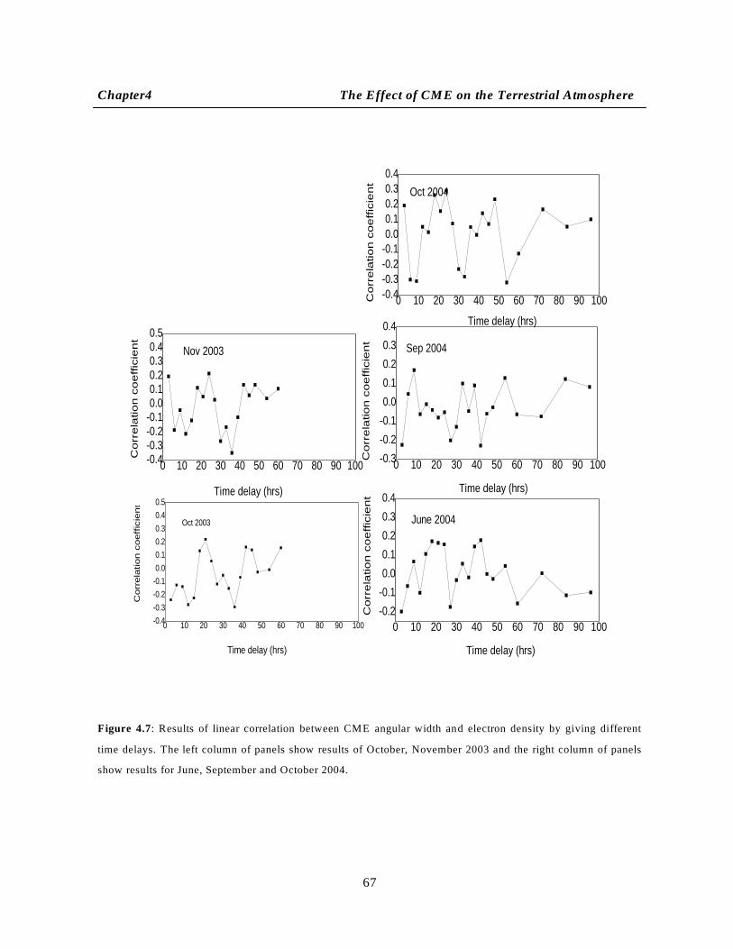
Figure 4.7: Results of linear correlation between CME angular width and electron density by giving different

time delays. The left column of panels show results of October, November 2003 and the right column of panels

show results for June, September and October 2004.

68


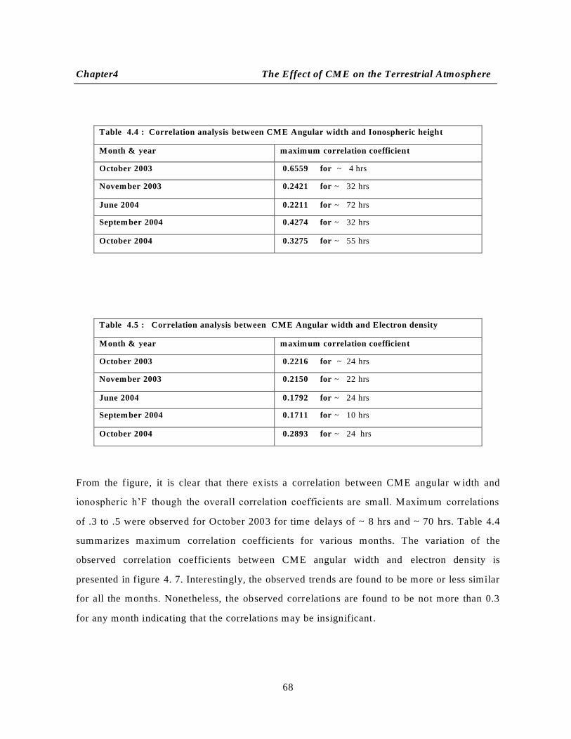
From the figure, it is clear that there exists a correlation between CME angular w idth and

ionospheric h‟F though the overall correlation coefficients are small. Maximum correlations

of .3 to .5 were observed for October 2003 for time delays of ~ 8 hrs and ~ 70 hrs. Table 4.4

summarizes maximum correlation coefficients for various months. The variation of the

observed correlation coefficients between CME angular width and electron density is

presented in figure 4. 7. Interestingly, the observed trends are found to be more or less similar

for all the months. Nonetheless, the observed correlations are found to be not more than 0.3

for any month indicating that the correlations may be insignificant.

Table 4.4 : Correlation analysis between CME Angular width and Ionospheric height




June 2004 0.2211 for ~ 72 hrs



Table 4.5 : Correlation analysis between CME Angular width and Electron density




June 2004 0.1792 for ~ 24 hrs



69


4.7 Correlation of CME Linear Speed and Angular Width with Solar W ind Speed

Solar wind is a stream of charged particles (a plasma) released from the sun. This

stream constantly varies in speed, density and temperature. The most dramatic difference in

these three parameters occurs when the solar wind escapes from a coronal hole or during a

coronal mass ejection. A stream originating from a coronal hole can be seen as a steady high -

speed stream of solar wind as where a CME is more like an enormous fast moving cloud of

solar plasma. During their propagation CMEs interact with solar wind and the interplanetary

magnetic field. The speed of the solar wind is an important factor. Particles with a higher

speed hit earth‟s magnetosphere harder and have a higher chance of causing disturbed

geomagnetic conditions. The solar wind speed at earth normally lies around 300km/s but

increases when a high speed Coronal Mass Ejection arrives. During a coronal mass ejection

impact, the solar wind speed can jump suddenly to 500, or even more than 1000km/s. As a

consequence slow CMEs are accelerated towards the speed of the Solar wind and the fast

CMEs are decelerated toward the speed of the Solar wind. Figures 4.8.& 4.9 clearly indicate

that there existed a good correlation between CME parameters and solar wind speed during

October/November2003.

0 10 20 30 40 50

0.0

0.1

0.2

0.3

0.4

0.5

0 10 20 30 40 50

0.0

0.1

0.2

0.3

0.4

0.5

0 10 20 30 40 50

0.0

0.1

0.2

0.3

0.4

0.5

0 10 20 30 40 50

0.0

0.1

0.2

0.3

0.4

0.5

Co

rre

latio

n c

oe

ffic

ien

t

Time delay (hrs)

June 2004

Co

rre

latio

n c

oe

ffic

ien

t

Time delay (hrs)

Oct 2004

Co

rre

latio

n c

oe

ffic

ien

t

Time delay (hrs)

Oct 2003

Co

rre

latio

n c

oe

ffic

ien

t

Time delay (hrs)

Nov 2003

Figure 4.8: Results of linear correlation between CME linear speed and Solar wind speed .The left column of

panels show results of October, November 2003 and the right column of panels show results for June and

October 2004.

70


But this correlation decreased in 2004. When we approach solar minimum there is

lesser number of CMEs and the coupling between the CME linear speed and Solar wind spe ed

gets weakened.

0 10 20 30 40 50

0.0

0.1

0.2

0.3

0.4

0.5

0 10 20 30 40 50

0.0

0.1

0.2

0.3

0.4

0.5

0 10 20 30 40 50

0.0

0.1

0.2

0.3

0.4

0.5

0 10 20 30 40 50

0.0

0.1

0.2

0.3

0.4

0.5

Co

rre

latio

n c

oe

ffic

ien

t

Time delay (hrs)

June 2004

Nov 2003

d e m o d e m o d e m o d e m o d e m o



Co

rre

latio

n c

oe

ffic

ien

t

Time delay (hrs)

Oct 2004d e m o d e m o d e m o d e m o d e m o




Oct 2003

Co

rre

latio

n c

oe

ffic

ien

t

Time delay (hrs)

d e m o d e m o d e m o d e m o d e m o d e m o




Co

rre

latio

n c

oe

ffic

ien

t

Time delay (hrs)




















Figure 4.9: Results of linear correlation between CME angular width and Solar wind speed .The left column of

panels show results of October, November 2003 and the right column of panels show results for June and

October 2004.

Table 4.6 : Correlation analysis between CME linear speed and Solar wind speed


October 2003 0.3799

November 2003 0.3890

June 2004 0.2938

October 2004 0.1365

71


4.8 Discussions

As can be seen from the analysis, it is the ionospheric height, and not the Electron

density, which exhibits significant correlations with the CME linear speed and angular spread.

The observed maximum correlation of 0.5 or more was found to be for October 2003 month

for a time delay of ~ 8hrs and ~ 70 hrs. The rationale for this is given as follows:

Over a dip equatorial station like Trivandrum, owing to the unique geomagne tic field

configuration the ionospheric height variations are purely due to the vertical plasma drift

caused by prevailing dynamo electrical field alone. In the initial /main phase of a storm the

main magnetospheric forcing that affects the ionosphere are m agnetospheric compression,

increase in the auroral electrojet heating, variation in the polar cap potential etc (Catherine and

Blanc, 1984). All these processes result in a modulation of the prevailing electrodynamical

coupling. For instance, the initial compression appears as the sudden commencement and

manifests as the height rise over the equator. On the other hand, variations in the polar cap

potential also maps to equator as prompt penetration field in the initial phase of a storm

(Balan et al., 2008). In this context, the observed time-delay of 8 hrs for maximum correlation

for October 2003 month corroborates with above understanding. In this context, the observed

time delay is indicative of the arrival of shock and resulting compression of magnetopaus e.

Further as the time progresses beyond 10 hrs or so, the composition, wind dynamics,

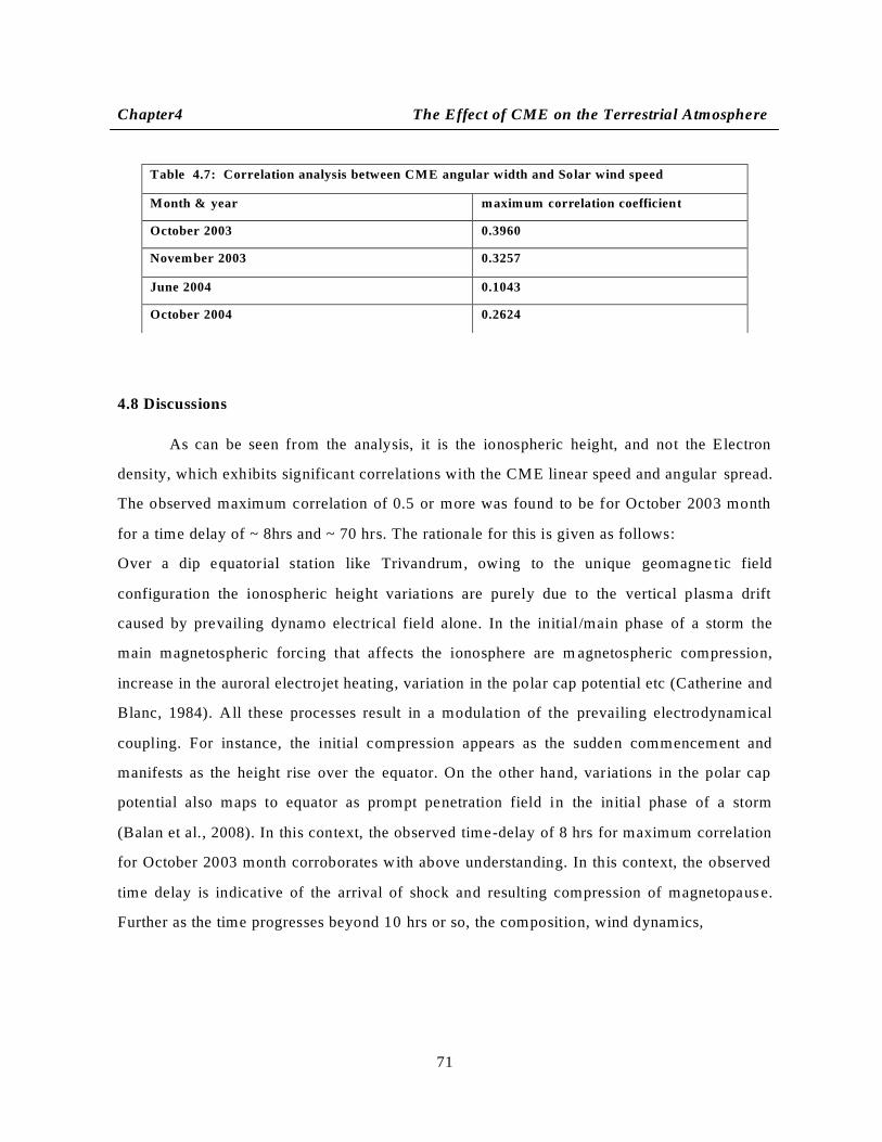
Table 4.7: Correlation analysis between CME angular width and Solar wind speed


October 2003 0.3960

November 2003 0.3257

June 2004 0.1043

October 2004 0.2624

72


and waves starts playing a role. As a consequence, thermospheric -ionospheric energetics and

dynamics gets modified. For instance, the disturbance dynamo gets active after about 30 -40

hrs or so. As mentioned earlier, over equator, the net result of the modified

energetics/dynamics manifests as an overall lowering of the prevailing electric field. In t his

context, the time delay of ~70 hrs is attributable to the time taken by the terrestrial upper

atmosphere to respond to the CME forcing in order to manifest in terms of variation in the

prevailing fields such as lowering of dynamo electric field over equator.

The electron density over the equatorial regions on the other hand, is influenced by a

lot of processes during storms e.g. meridional wind circulation and composition changes,

EIA.diffusion etc. As a consequence, the ionospheric density is expected to exhibit a small, or

no, correlation at all with the CME parameters. Also there exists a good correlation between

CME parameters and Solar wind speed during October/ November 2003 .

4.9 Concluding remarks

In this chapter focus was on the effects of CMEs on the equatorial geomagnetic activity

based on the correlation between CME parameters (linear speed and angular width) with

ionospheric parameters (h‟F and electron density) and Solar wind speed. Although effects of

CMEs on ionosphere have been studied since the 1950s, this work is different in its approach.

We found that the CME parameters (linear speed & angular width) display significant

correlations primarily with ionospheric height h‟F. The highest correlation observed during

the month October 2003 for a time delay of about 8 hrs is due to the passage of the ICME and

the shock associated with it while time delay of ~72 hrs indicates the time taken by terrestrial

upper atmosphere over equator to respond to CME forcing. Our analysis reveals that CME

(linear speed and angular width) could play a major role in modulating the ionospheric height

variations over the equator for short periods (a few hours) as well as for a long time scale

(days).

chapter 4shodhganga.inflibnet.ac.in/bitstream/10603/42092/14/14... · 2018-07-03 · 49 chapter 4...

Documents