chapter 3: metrics

Chapter 3: Metrics

Roger Grosse

1 Introduction

Last week, we looked at the Hessian, which defines the second-order Taylorapproximation to the cost function in neural network training. This week,we’ll look at a different but closely related type of second-order Taylorapproximation. Here, we’re interested in approximating some notion ofdistance between two weight vectors. One way to measure distance is usingEuclidean distance in weight space (which there’s no need to approximate).But we can define lots of other interesting distances, and taking a second-order Taylor approximation to such a distance gives a metric.

To motivate why we are interested in metrics, consider the Rosenbrockfunction (Figure 1), which has been used for decades as a toy problem inoptimization:

h(x1, x2) = (a− x1)2 + b(x2 − x21)2

This function is hard to optimize because its minimum is surrounded by anarrow and flat valley, in which gradient descent gets stuck (Figure 1).

One interesting way of looking at the Rosenbrock function is that it’sreally the composition of two functions: a nonlinear mapping, and squaredEuclidean distance:

J (x1, x2) = L(f(x1, x2))

f(x1, x2) = (a− x1,√b(x2 − x21))

L(z1, z2) = z21 + z22 .

Here, we refer to (x1, x2) as the input variables, and (z1, z2) as the outputvariables. The loss L is just squared Euclidean distance. It’s the nonlineartransformation that makes the optimization difficult. Figure 1(a,b) showsthe optimization trajectory in input space and output space, respectively.This general setup, where we are trying to minimze a composition of func-tions, is known as composite optimization.

This setup is roughly analogous to neural net training: (x1, x2) are likethe weights of the network, and (z1, z2) are like the outputs of the network.Typically, we assign a simple, convex loss function in output space, such assquared error or cross-entropy. It’s the nonlinear mapping between weightsand outputs that makes the optimization difficult. The main place theanalogy breaks down is that the neural net cost function is summed overmultiple training examples, and the nonlinear mapping (from weights tooutptuts) is different each time.

The output loss (L as a function of (z1, z2)) is probably the easiest func-tion in the world to optimize. Figure 1(c,d) shows what would happen if we

1

CSC2541 Winter 2021 Chapter 3: Metrics

(a) (b) (c) (d)

Figure 1: Gradient descent on the Rosenbrock function. (a) Gradient descent in input space bouncesacross the valley and makes slow progress towards the optimum, due to ill-conditioning. (b) The corre-sponding trajectory in output space. (c,d) The parameter space and output space trajectories for gradientdescent on the outputs.

could do gradient descent directly on the outputs (z1, z2). For this particularfunction, “gradient descent on the outputs” at least makes conceptual sensebecause the mapping f is invertible. The optimization trajectory darts di-rectly for the optimum (and, in fact, would reach it exactly in 1 step if weused a step size of 1). This is cheating, of course, but it provides us withan idealized optimizer we can try to approximate.

Unfortunately, this notion of “gradient descent on the outputs” doesn’tapply to lots of other situations we care about, such as neural net training.One problem is that the neural net function is generally not invertible: theremight not be any weight vector that produces a given set of outputs on thetraining set, or there might be many such weight vectors. In the latter case,it generally won’t be easy to find such a weight vector. Even if we could, thefact that it performs well on the training set gives us no guarantee aboutits generalization performance.

However, there’s another way to define “gradient descent on the out-puts” which does carry over to neural nets. In particular, we’ll considerproximal optimization, where we minimize the cost function (or an approxi-mation therof), plus a proximity term which penalizes how far we’ve movedfrom the previous iterate. Proximal optimization is especially interestingif we measure proximity in function space. Approximating function spaceproximity gives rise to a useful class of matrices known as pullback metrics.

As part of this investigation, we’ll look at how to measure dissimilaritybetween probability distributions. A natural dissimilarity measure betweendistributions is KL divergence, and taking the second-order Taylor approx-imation gives us the ubiquitous Fisher information matrix. When the dis-tributions are exponential families, this gives rise to an especially beautifulset of mathematical identities.

2 Proximal Optimization

We’ll now turn to a class of optimization algorithms known as proximalmethods. This refers to a general class of methods where in each step weminimize a function plus a proximity term which penalizes the distance fromthe current iterate. While there are some practical optimization algorithmsthat explicitly use proximal updates, we’ll instead use proximal optimiza-

2


tion as a conceptual tool for thinking about optimization algorithms. We’llstart by defining idealized proximal updates which do something interest-ing but are impractical to compute, and then figure out how to efficientlyapproximate those updates.

Suppose we’re trying to minimize a function J (w). The idealized updaterule, known as the proximal point method, is as follows:

w(k+1) = proxJ ,λ(w(k)) = arg minu

[J (u) + λρ(u,w(k))

], (1)

where ρ is a dissimilarity function which, intuitively, measures the dis-tance between two vectors, but doesn’t need to satisfy all the axioms ofa distance metric. Canonical examples include squared Euclidean distanceand KL divergence. The term λρ(u,w(k)) is called the proximity term,and the operator proxf,λ is called the proximal operator. To make thismore concrete, let’s consider some specific examples.

To begin with, let’s measure dissimilarity using squared Euclidean dis-tance:

ρ(u,v) = 12‖u− v‖2.

Plugging this into Eqn. 1, our proximal operator is given by:

proxJ ,λ(w(k)) = arg minu

[J (u) + λ

2‖u−w(k)‖2]. (2)

If J is differentiable and convex and λ > 0, then the proximal objective isstrongly convex, so we can find the optimum by setting the gradient to 0:

∇J (u?) + λ(u? −w(k)) = 0.

Rearranging terms, we get an interesting interpretation of the optimalitycondition:

proxJ ,λ(w(k)) = u? = w(k) − λ−1∇J (u?). (3)

This resembles the gradient descent update for J , except that the gradientis computed at the new iterate rather than the old one. This equation isnot an explicit formula for u? because u? appears on the right-hand side;hence, it is known as the implicit gradient descent update.

Clearly it can’t be very easy to compute the implicit gradient descentupdate, since setting λ = 0 drops the proximity term, so proxJ ,0 simplyminimizes J directly. Hence, exactly solving the proximal objective ingeneral is as hard as the original optimization problem.

We can make some approximations, however. The first such approxima-tion is to linearize the cost. Returning for a moment to the general proximalobjective (Eqn. 1), suppose we linearize J around the current iterate w(k):


[J (w(k)) +∇J (w(k))>(u−w(k)) + λρ(u,w(k))

]= arg min

u

[∇J (w(k))>u + λρ(u,w(k))

]Setting the gradient to 0, we get the following optimality conditions:

∇uρ(u?,w(k)) = −λ−1∇J (w(k)).

3


For some choices of ρ, this gives an algorithm known as mirror descent— a term whose meaning will later become clear. For squared Euclideandistance, ∇uρ(u,v) = u − v, so mirror descent reduces to the ordinarygradient descent update:

u? = w(k) − λ−1∇J (w(k)).

A second approach is to take the infinitesimal limit by letting λ → ∞.If the proximity term is weighted extremely heavily, then u? will remainclose to w(k). Hence, J will be well-approximated by the first-order Taylorapproximation, just as above. Now consider approximating ρ. First of all,since ρ(u,v) is minimized when u = v, we have ∇uρ(u,v)

∣∣u=v

= 0. Hence,we approximate it with the second-order Taylor approximation,

ρ(u,w(k)) = 12(u−w(k))>G(u−w(k)) +O(‖u−w(k)‖3)

where G = ∇2uρ(u,w(k))

∣∣u=w(k) is known as the metric matrix. This

formula can also be written in terms of a class of distance metrics calledMahalanobis distance, which you can visualize as a stretched-out versionof Euclidean distance:

ρ(u,w(k)) = 12‖u−w(k)‖2G +O(‖u−w(k)‖3)

‖v‖G =√

v>Gv.

Plugging both approximations into Eqn. 1, we get:


[∇J (w(k))>u + λ

2 (u−w(k))>G(u−w(k))],

with optimumu? = w(k) − λ−1G−1∇J (w(k)). (4)

This optimal solution resembles the Newton update w(k)−αH−1∇J (w(k)),except that H (the Hessian of J ) is replaced by G (the Hessian of ρ). Inthe case where ρ represents squared Euclidean distance, G = I, so thissolution also reduces to the ordinary gradient descent update. Since we’re considering the λ→∞

limit, this implies that implicitgradient descent behaves likeordinary gradient descent whenthe steps are small enough.

In general,however, we’ll see that these two approximations can yield interestinglydifferent algorithms.

Finally, a third approach is to take a second-order Taylor approxima-tion to J and a second-order Taylor approximation to ρ. This might bemore accurate than the previous approximation for larger step sizes, be-cause we’re using a second-order rather than first-order approximation toJ . The update rule, derived similarly to the ones above, is given by:

w(k+1) = w(k) − (H + λG)−1∇J (w(k)). (5)

If ρ is chosen to be squared Euclidean distance, then G = I, and this givesa damped Newton update. Intuitively, the damping term prevents theoptimizer from taking a very large step in low curvature directions, perhapshelping to stabilize the optimization. We won’t consider this particularapproximation any further in today’s lecture, but we’ll discuss the role ofdamping in more detail next week, when we talk about second-order opti-mization of neural nets.

4


2.1 Trust Region Methods

Proximal methods are also closely related to another family of optimiza-tion algorithms known as trust region methods. Here, the soft proximitypenalty is converted to a hard constraint:

arg minu

J (u) s.t. ρ(u,w(k)) ≤ η, (6)

where η is a hyperparameter controlling how far each update is allowedto wander from the current iterate. If J is convex, then the trust regionproblem is actually equivalent to the proximal problem, in the sense thatany optimum to Eqn. 6 is also an optimum to Eqn. 1 for some value of λ,and vice versa. The difference between these approaches is simply whetheryou’d prefer to control the size of the updates directly, or control the weightof the proximity term.

3 Fisher Information

So far, our only example of proximal updates used the Euclidean metric,which isn’t that interesting because the results agree with the ordinary gra-dient. Proximal updates become much more powerful if we can use a moreintrinsically meaningful dissimilarity function. In the case of probabilitydistributions, a natural dissimilarity function is KL divergence:

DKL(q ‖ p) = Ex∼q[log q(x)− log p(x)] (7)

KL divergence isn’t truly a distance metric, because it it asymmetric anddoesn’t satisfy the triangle inequality. Actually, KL divergence is more

closely analogous to squaredEuclidean distance than toEuclidean distance. However,√

DKL doesn’t satisfy symmetry orthe triangle inequality either.

However, it’s very convenient as away of measuring how different two distributions are. For instance, it hasthe information theoretic interpretation as relative entropy, i.e. the numberof bits wasted if you try to encode data from source q using a code de-signed for another source p. It can be shown that DKL is nonnegative, andDKL(q ‖ q) = 0 for any distribution q — basic properties we need from anydissimilarity function. For a great tutorial introduction to

KL divergence, seehttps://colah.github.io/posts/

2015-09-Visual-Information/.

Notice that Eqn. 7 doesn’t mention the parameters of the distributions.That’s because KL divergence is an intrinsic dissimilarity function betweendistributions, i.e. it doesn’t care how they’re parameterized. But if we’retrying to learn a distribution, we’ll typically restrict ourselves to some para-metric family {pθ} (such as Gaussians), parameterized by θ.

Recall that when we derived approximations to the proximal operators,we sometimes needed the Hessian of the dissimilarity function. For ρ =DKL, this is given by the Fisher information matrix, denoted Fθ. (Thesubscript indicates the parameterization, but we’ll drop it when it’s obviousfrom context.) Exercise: derive these expressions

for Fθ.∇2uDKL(pu ‖ pθ)

∣∣u=θ

= Fθ

= Covx∼pθ(∇θ log pθ(x))

= Ex∼pθ

[(∇θ log pθ(x))(∇θ log pθ(x))>

] (8)

The second and third lines give explicit formulas for Fθ in terms of the log-likelihood gradients ∇θ log pθ(x), which are called the Fisher scores. The

5

https://colah.github.io/posts/2015-09-Visual-Information/

https://colah.github.io/posts/2015-09-Visual-Information/


third equality follows from the general identity (which applies to any ran-dom vector v):

Cov(v) = E[vv>]− E[v]E[v]>,

combined with the observation that The fact thatEx∼pθ [∇θ log pθ(x)] = 0 can beproved using integration by parts.But the intuition is that the trueparameters θ maximize theexpected log-likelihood for datadrawn from pθ, so thelog-likelihood gradient should be 0in expectation.

Ex∼pθ [∇θ log pθ(x)] = 0.

The explicit formulas for Fθ may be more familiar from a statistics classthan the interpretation as the Hessian of DKL. But I’d argue that theHessian of DKL is really the right way to think about Fθ, i.e. it defines alocal distance metric in the space of distributions.

So the exact proximal update is as follows:

proxJ ,λ(θ) = arg minu

[J (u) + λDKL(pu ‖ pθ)] . (9)

Let’s take the infinitesimal limit, i.e. λ → ∞, given by Eqn. 4. This givesthe following update:

θ(k+1) = θ − αF−1θ ∇J (θ)

= θ − α∇J (θ),(10)

where α = λ−1 and the vector ∇J (θ) = F−1θ ∇J (θ) is the natural gra-dient. This update rule is known as natural gradient descent. Theterm natural comes from the fact that the update is independent of howthe distribution is parameterized, up to the first order. More on this inSection 6.

4 Exponential Families

The above discussion applies to any parametric family of distributions. The discussion of exponentialfamilies can be skipped withouttoo much loss of continuity. Butit’s so beautiful that I just had toinclude it.

Butwe get some very interesting interpretations of natural gradient when we spe-cialize to particular classes of distributions known as exponential families.In general, an exponential family is a family of probability distributions thathas the following form:

pη(x) =h(x)

Z(η)exp

(η>t(x)

), (11)

where η are the natural parameters of the distribution, and t is a vectorof sufficient statistics. (We’ll see where this term comes from when wediscuss maximum likelihood.) The factor 1/Z(η) is known as the normal-izing constant because its role is to ensure that the PDF integrates to 1,and Z(η) is the partition function, defined as

Z(η) =

∫h(x) exp

(η>t(x)

)dx or

Z(η) =∑x

h(x) exp(η>t(x)

),

(12)

depending if the distribution is continuous or discrete.

6


The moments of an exponential family distribution are the expectedsufficient statistics:

ξ = Ex∼pη [t(x)].

Under some regularity conditions, it can be shown that there is a one-to-one mapping between the moments and the natural parameters. Hence, ξcan be seen as an alternative parameterization of the exponential family, inwhich case we write pξ.

Now let’s see some concrete examples of exponential families.

1. The Bernoulli distribution, where x ∈ {0, 1}, and Pr(x = 1) = θ. Thiscan be seen as an exponential family with ξ(x) = x and h(x) = 1. Themoment is E[ξ(x)] = θ. It can be shown that the natural parameterssatisfy:

η = logθ

1− θθ = σ(η) =

1

1 + exp(−η).

Hence, the natural parameter represents the logit, which gives the logodds ratio between the two outcomes. The moment is obtained fromthe natural parameters using the logistic function σ, a standardneural network activation function. It’s common to use the logisticactivation function for the output layer in binary classification (eitherwith neural nets or logistic regression), so the output pre-activationscan be seen as the natural parameters, and the output activations asthe moments.

2. The categorical distribution, where x is a one-hot vector, i.e. abinary vector with exactly one entry being 1, and the vector θ rep-resents the probabilities of each outcome. This is a generalization ofthe Bernoulli distribution to more than 2 possible outcomes. It canbe seen as an exponential family with t(x) = x and h(x) = 1. Themoments are E[t(x)] = θ. The natural parameters can be defined as:

ηi = log θi θi = [σ(η)]i =exp(ηi)∑j exp(ηj)

.

The function σ is the softmax function, the standard activationfunction for output layers of a classification network. This shows thatthe natural parameters η, called the logits, can be seen as the logodds ratios of the outcomes.

This representation is good enough for many purposes. However, it’snot a minimal exponential family, since the sufficient statistics arelinearly dependent (the entries always sum to 1). This can be fixedby truncating the final coordinate of the one-hot vector, so that theKth class is arbitrarily assigned to 0. The formulas are a bit morecumbersome, but basically similar to the ones given above.

3. Now consider a Gaussian distribution with fixed covariance Σ, param-eterized by the mean vector µ:

pµ(x) =1

(2π)D/2|Σ|1/2exp

(−1

2(x− µ)>Σ−1(x− µ))

=1

(2π)D/2|Σ|1/2exp

(−1

2x>Σ−1x + µ>Σ−1x− 12µ>Σ−1µ

)

7


This is an exponential family distribution with sufficient statisticst(x) = x, natural parameters h = Σ−1µ (also called the poten-tial vector), and moments ξ = E[t(x)] = µ. Hence, in this instance,the natural parameters and sufficient statistics are equivalent, up toa linear transformation. You can check that: This parameterization might seem

a little weird, which just showsthat the natural parameters aren’talways the most “natural” way toparameterize a distribution.

h(x) = exp(−12x>Σ−1x)

Z(h) = (2π)D/2|Σ|1/2 exp(−12h>Σh)

4. Now make the Gaussian zero-mean, but parameterize it by the covari-ance matrix Σ. This is an exponential family with sufficient statisticst(x) = −1

2 vec(xx>), natural parameters η = vec(Σ−1), and momentsξ = E[t(x)] = −1

2 vec(Σ). Our formulation of Gaussians hereis not a minimal exponentialfamily. To make it minimal, weshould instead extract the uppertriangular entries of Λ and xx>.

The notation vec denotes the Kroneckervectorization operator which stacks the columns of a matrix into avector. The matrix Λ = Σ−1 is called the precision matrix; it isa positive definite matrix which, intuitively, is large in the directionswhere the distribution is the most constrained (i.e. most “precise”).

5. Finally, let’s put this together by considering a general Gaussian dis-tribution parameterized by both µ and Σ. To make the exponentialfamily interpretation more obvious, we can rewrite the Gaussian PDFin another form called information form:

ph,Λ(x) =|Λ|1/2

(2π)D/2exp

(−1

2x>Λx + h>x− 12h>Λ−1h

).

The sufficient statistics, natural parameters, and moments are givenby:

t(x) =

(x

−12 vec(xx>)

)η =

(h

vec(Λ)

)ξ =

(µ

−12 vec(Σ + µµ>)

)Hence, the natural parameters are exactly the information form pa-rameters, reshaped into a vector, and the moments are (proportionalto) the first and second moments of the distribution. The momentsaren’t quite the same as the standard parameterization in terms ofµ and Σ (which is known as covariance form), but each is easilyobtainable from the other.

Covariance form and information form are two fundamental param-eterizations of the Gaussian distribution. Converting between themrequires a matrix inversion (to compute Λ from Σ or vice versa),which is an O(D3) operation. For many applications, this inversion isfeasible but expensive, hence we’d like to do it as rarely as possible.Hence, algorithms based on manipulating Gaussian distributions arecarefully designed to carry out some steps in information form andsome steps in covariance form in order to minimize the number of in-versions. This is crucial in, e.g., Kalman filtering and Gaussian beliefpropagation.

The innocuous-looking partition function Z(η) is the source of manyelegant identities involving exponential families.

8


1. First of all, we get a nice formula for the moments:

ξ = ∇ logZ(η). (13)

This is nice because we have convenient automatic differentiationtools, but not convenient tools for computing expectations. This iden-tity means we can obtain the moments simply by writing a functionthat computes logZ(η), and then calling grad on it.

2. The formula for the log-likelihood is:

`(η) =N∑i=1

log pη(x)

=N∑i=1

[η>t(x(i))− logZ(η)

],

(14)

and its gradient is

∇η log pη(x) = t(x)− ξ (from Eqn. 13)

∇`(η) = ξ − ξ

ξ =1

N

N∑i=1

t(x(i)),

(15)

where ξ is called the empirical moments. Setting the gradient to0, we find that the likelihood is maximized when ξ = ξ. You can check that this formula is

consistent with the well-knownmaximum likelihood estimates forBernoulli, categorical, andGaussian distributions.

This impliesthat, to compute the maximum likelihood parameters, we only needto store ξ, and can otherwise forget the data; this is why t is called thesufficient statistic. Since maximum likelihood involves matching themodel moments to the empirical moments, this is known as momentmatching.

3. We just saw that ∇η log pη(x) = t(x)−ξ (see Eqn. 15). Plugging thisinto Eqn. 8, we get a convenient formula for the Fisher informationmatrix:

Fη = Covx∼pη(t(x)) (16)

4. The KL divergence is given by:

DKL(pη1‖ pη2

) = Ex∼pη1[log pη1

(x)− log pη2(x)]

= Ex∼pη1[η>1 t(x)− η>2 t(x)]− logZ(η1) + logZ(η2).

Taking the Hessian with respect to η2, all of the linear and constantterms drop out, and we’re left with just ∇2 logZ(η2). But the Hessianof KL divergence is Fη (Eqn. 8). So this gives us a neat identity

Fη = ∇2 logZ(η). (17)

Just like Eqn. 13 gave us a convenient way to compute ξ in an autodiffframework, Eqn. 17 gives us a convenient way to compute F: just takethe function that computes logZ(η) and call grad on it twice. (Or, ifyou don’t want to construct the full matrix, you can compute MVPswith F by computing Hessian-vector products with logZ.)

9


5. As a consequence of Eqn. 17, the Hessian of the negative log-likelihoodis also Fη:

∇2η log pη(x) = ∇2

η[η>t(x(i))]︸︷︷︸=0

−∇2η logZ(η)

= −Fη.

(18)

This implies that the natural gradient descent update for maximumlikelihood estimation in exponential families is the same as the Newton-Raphson update (up to a scale factor).

6. We saw that ξ = ∇ logZ(η) and Fη = ∇2 logZ(η). But since theHessian is just the gradient of the gradient, this implies:

Fη = ∇ξ(η) = Jξ,η, (19)

where Jξ,η denotes the Jacobian of the mapping from natural param-eters to moments. Another way to write this is:

dξ = Fηdη,

where dξ and dη denote infinitesimal perturbations to the momentsand natural parameters, respectively. Note that the Jacobian of theinverse mapping is just Jη,ξ = F−1η . This is a surprisingly usefulidentity, and shows that the Fisher information matrix fundamentallyrelates the two coordinate systems.

We’ve just seen a number of beautiful identities relating two coordinatesystems for exponential families — natural parameters and moments — andthey all somehow pass through logZ. This is no accident: the relationshipbetween natural parameters and moments is a special case of Legendreduality, and there’s a beautiful field called information geometry whichexplores these sorts of ideas. Amari and Nagaoka (2000) is the classic texton this topic, and Amari (2016) is more up-to-date though less polished.

4.1 Proximal Operators in Exponential Families

When we compute the proximal operator for an exponential family usingKL divergence as the dissimilarity function, something neat happens. First,suppose we take the first-order approximation to the cost function, but keepthe proximal term exact. In this section, we’ll use Jη and

Jξ to denote the cost function,viewed as a function of η or ξ.

Then we’re minimizing:

∇Jη(η(k))>u + λDKL(pη(k) ‖ pu).

Computing the gradient with respect to u and setting it to 0, we find that:

ξ(k+1) = ξ(k) − λ−1∇Jη(η(k)). (20)

In other words, the moments are updated opposite the gradient computedfor the natural parameters!

Similarly, suppose we use the opposite direction of KL divergence forthe proximity term. Here, it’s more convenient to use the moments param-eterization, so let J denote the cost function parameterized in terms of themoments. Then we’re minimizing:

∇Jξ(ξ(k))>u + λDKL(pu ‖ pξ(k)).

10


Computing the gradient with respect to u and setting it to 0, we find that:

η(k+1) = η(k) − λ−1∇Jξ(ξ(k)). (21)

So we update the natural parameters opposite the gradient computed forthe moments! These two update rules, where you compute the gradient inone coordinate system and then apply it in the other coordinate system, areknown as mirror descent.

Now we show that the natural gradient update is equivalent to mirrordescent. By the Chain Rule for derivatives, we have: You can also see that natural

gradient descent is equivalent tomirror descent by taking the limitof Eqns. 20 and 21 as λ→∞.

∇ηJη(η) = ∇ηJξ(ξ(η))

= J>ξ,η∇ξJξ(ξ(η))

= Fη∇ξJξ(ξ(η)) (Eqn. 19)

Multiplying both sides by F−1η , we get a surprising formula for the naturalgradient:

∇ηJη(η) = F−1η ∇ηJη(η) = ∇ξJξ(ξ(η)). (22)

Similarly, it can be shown that

∇ξJξ(ξ) = ∇ηJη(η(ξ)). (23)

So the natural gradient with respect to the natural parameters is the ordi-nary Euclidean gradient with respect to the moments, and vice versa!

Why is this connection useful? For one thing, it’s often the easiest wayto derive the natural gradient update in practice. E.g., suppose you want tocompute the natural gradient update for a multivariate Gaussian distribu-tion with unknown mean and covariance. If you’re feeling masochistic, youcould do this by representing the Gaussian as a minimal exponential fam-ily (i.e. taking the upper triangular entries of Σ, etc.) and then somehowderiving an expression for F. Sound fun? Or you can solve it more simplyby applying Eqns. 22 or 23.

4.2 Maximum Likelihood and Fisher Efficiency

Now we’ll consider a case where natural gradient descent — and, equiva-lently, mirror descent — clearly does the right thing: maximum likelihoodin exponential families. Here, we’re trying to maximize the log-likelihood(Eqn. 14), for which the optimal solution is given by moment matching,ξ = ξ (Eqn. 15). This can clearly be done by sweeping once over the train-ing set to compute ξ. But what if we do natural gradient descent instead?

We’ll consider the online learning setting, where we iterate once throughthe training set, updating on one training example at a time. The log-likelihood gradient for a single example is given by (see Eqn. 15):

∇η log pη(x) = t(x)− ξ

By plugging this into Eqns. 20 and 23, we see that the mirror descent update,and the natural gradient update for ξ, are both given by:

ξ(k+1) = ξ(k) − αk(ξ(k) − t(x(k+1))). (24)

11


I write αk rather than α so that we can choose a learning rate schedule,i.e. a different learning rate for each time step. An interesting choice ofschedule is αk = 1/k. You can show by induction that this update computesa running average of the empirical moments:

ξ(k) =1

k

k∑i=1

t(x(i)). (25)

In other words, the kth iterate is exactly the batch maximum likelihoodestimate of the parameters from the first k examples! As a special case,once the entire dataset is processed, we have the exact maximum likelihoodestimate ξ(N) = ξ.

This is interesting because the batch maximum likelihood estimate is atrick which only applies to exponential families, while mirror descent andnatural gradient descent are generic algorithms that can be applied to lotsmore cost functions. The property that the online algorithms come closeto the information theoretic optimum is known as Fisher efficiency, andAmari (1998) showed that natural gradient descent is Fisher efficient in awider variety of situations than just maximum likelihood. In Chapter 7,we’ll derive a result closely related to Amari’s analysis of natural gradientdescent.

The mirror descent and natural gradient updates for maximum likeli-hood have the property that each update results in a statistically optimalinference from the information seen so far. Algorithms which incremen-tally update a probabilistic model as new information arrives are knownas filtering algorithms. Natural gradient descent can be interpreted as afiltering algorithm in a wider variety of situations, although typically thecorrespondence is only approximate (Ollivier, 2018).

5 Approximating Function Space Proximity

We’ve just seen two examples of dissimilarity functions: squared Euclideandistance, and KL divergence. Between these, only squared Euclidean dis-tance is directly applicable to neural nets. (KL divergence is for probabilitydistributions, and a neural net isn’t a probability distribution.) But Eu-clidean distance in weight space is unappealing, because it depends on anarbitrary parameterization of the network (see Section 6) and because itneglects the fact that some directions in weight space can have a muchlarger effect than others on the network’s predictions. When dealing withprobability distributions, a convenient property of KL divergence is that itis natural : it depends only on the distributions themselves, not how they’reparameterized. Can we define natural dissimilarity functions for neuralnets?

The mathematical operation we’ll use to do this is called pullback.The general idea is simple: if we have a differentiable map z = f(x) and afunction g(z1, . . . , zK) To clarify the notation: f∗ is an

operator. When we write f∗g(· · · ),this means we first evaluate f∗g(which gives us a function), andthen we evaluate this function onthe arguments in parentheses.

defined on the output space, then the pullback of gover f, denoted f∗g, is defined as follows:

f∗g(x1, . . . ,xK) = g(f(x1), . . . , f(xK)). (26)

12


(a) (b) (c)

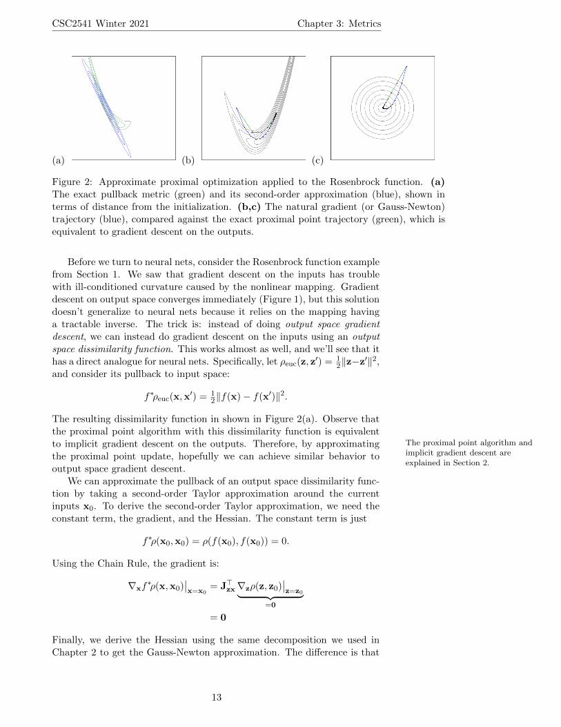
Figure 2: Approximate proximal optimization applied to the Rosenbrock function. (a)The exact pullback metric (green) and its second-order approximation (blue), shown interms of distance from the initialization. (b,c) The natural gradient (or Gauss-Newton)trajectory (blue), compared against the exact proximal point trajectory (green), which isequivalent to gradient descent on the outputs.

Before we turn to neural nets, consider the Rosenbrock function examplefrom Section 1. We saw that gradient descent on the inputs has troublewith ill-conditioned curvature caused by the nonlinear mapping. Gradientdescent on output space converges immediately (Figure 1), but this solutiondoesn’t generalize to neural nets because it relies on the mapping havinga tractable inverse. The trick is: instead of doing output space gradientdescent, we can instead do gradient descent on the inputs using an outputspace dissimilarity function. This works almost as well, and we’ll see that ithas a direct analogue for neural nets. Specifically, let ρeuc(z, z

′) = 12‖z−z′‖2,

and consider its pullback to input space:

f∗ρeuc(x,x′) = 1

2‖f(x)− f(x′)‖2.

The resulting dissimilarity function in shown in Figure 2(a). Observe thatthe proximal point algorithm with this dissimilarity function is equivalentto implicit gradient descent The proximal point algorithm and

implicit gradient descent areexplained in Section 2.

on the outputs. Therefore, by approximatingthe proximal point update, hopefully we can achieve similar behavior tooutput space gradient descent.

We can approximate the pullback of an output space dissimilarity func-tion by taking a second-order Taylor approximation around the currentinputs x0. To derive the second-order Taylor approximation, we need theconstant term, the gradient, and the Hessian. The constant term is just

f∗ρ(x0,x0) = ρ(f(x0), f(x0)) = 0.

Using the Chain Rule, the gradient is:

∇xf∗ρ(x,x0)

∣∣x=x0

= J>zx∇zρ(z, z0)∣∣z=z0︸︷︷︸

=0

= 0

Finally, we derive the Hessian using the same decomposition we used inChapter 2 to get the Gauss-Newton approximation. The difference is that

13


this time the formula is exact because the second term is 0:

∇2xf∗ρ(x,x0)

∣∣x=x0

= J>zx

[∇2

zρ(z, z0)∣∣z=z′

]Jzx +

∑a

∂ρ

∂za∇2

x[f(x)]a︸︷︷︸=0

= J>zxGzJzx,

. (27)

where Gz = ∇2zρ(z, z0)|z=z0 is the output space metric matrix. In the first

line, the reason the second term drops out is that it contains the outputspace partial derivatives ∂ρ/∂ya, which are 0. Hence, our second-orderTaylor approximation to the pullback f∗ρ(x,x0) is the Mahalanobis metric:

f∗ρ(x,x0) ≈ 12‖x− x0‖2Gx

= 12(x− x0)

>Gx(x− x0),

where Gx = J>zxGzJzx. In general, we’ll drop the subscripts on Gx whenit’s clear from context which metric matrix we’re referring to.

For our Rosenbrock example, we chose squared Euclidean distance onoutput space. Hence, Gz = I, and Gx = J>zxJzx turns out to equal theGauss-Newton matrix (see Chapter 2). The connection with the

Gauss-Newton Hessian is discussedfurther in Section 5.1.

The natural gradient updates, there-fore, are equivalent to the Gauss-Newton updates up to a scale factor:

x(k+1) = x(k) − αG−1x ∇J (x(k)). (28)

The natural gradient (or Gauss-Newton) trajectory is shown in Figure 2(b,c).While it doesn’t exactly match the output space gradient descent trajectory,it has a qualitatively similar behavior, and in particular doesn’t get stuckbouncing across the valley the way gradient descent does (Figure 1(a,b)).

Now let’s generalize this to neural nets (and function approximationmore generally). Here, we’ll measure the dissimilarity between two weightvectors by how different the networks’ outputs are in expectation. Often it’spossible to choose a meaningful dissimilarity function ρ on output space,such as squared Euclidean distance:

ρ(z, z′) = 12‖z− z′‖2.

The distance between weight vectors, then, can be measured in terms of theaverage dissimilarity between the outputs, taken with respect to the datadistrubution. This is referred to informally as function space distance.Letting fx(w) = f(w,x), we define: In weight space, ρpull is only a

semimetric, not a metric, becauseit may be 0 for distinct weightvectors. This distinction won’tconcern us.

ρpull(w,w′) = Ex[f∗xρ(w,w′)] = Ex[ρ(f(w,x), f(w′,x))].

or its finite sample version:

ρpull(w,w′) =

1

N

N∑i=1

[ρ(f(w,x(i)), f(w′,x(i)))].

This notion of function space distance is illustrated in Figure 3.Now consider the second-order Taylor approximation to ρpull:

∇2wρpull(w,w

′)∣∣w=w′

= Ex

[∇2

wρ(f(w,x), f(w′,x))]

= Ex[J>zwGzJzw].(29)

14


Figure 3: Illustration of function space distance. If we have a 1-D regressionproblem with 4 training examples, the function space distance between twofunctions is approximated as the mean of the squared distances between thepredictions on these 4 training inputs.

(The derivation follows Eqn. 27). As before, Gz = ∇2zρ(z, z′) is the metric

matrix for output space.We denote the weight space metric matrix as G = ∇2

wρpull(w,w′)∣∣w=w′

(or Gw when we want to distinguish it from other metric matrices) becausethe letter g is traditionally used to denote metrics in Riemannian geometry.

For those who are familiar withRiemannian geometry, notice analternative way to construct Gw:we could have instead defined aRiemannian metric on outputspace and pulled it back to weightspace over f . This gives anotherway to understand the termpullback metric.

I’ll refer to it as the pullback metric, because it’s constructed using thepullback operation. (This isn’t a standard term, but no standard term hasyet been adopted.) The choice of the letter G collides with our notationfor the Gauss-Newton Hessian (see Chapter 2), but that’s OK because we’llnow see that the two matrices are equivalent in a lot of important situations.

5.1 Connection to the Gauss-Newton Hessian

In our Rosenbrock example, we saw that the pullback metric for Euclideandistance agrees with the classical Gauss-Newton matrix (see Eqn. 28). Thisis a special case of a more general relationship. Given a strictly convex func-tion φ, the Bregman divergence between two points z and z′ is definedas:

Dφ(z, z′) = φ(z)− φ(z′)−∇φ(z′)>(z− z′).

We can understand this geometrically as follows (see Figure 4). Because φis convex, the first-order Taylor approximation to φ at z′ is a lower boundon φ. The further a point is from z′, the less accurate the lower bound willbe. The Bregman divergence Dφ(z, z′) is simply the gap between φ(z) andthe lower bound.

Like KL divergence, Bregman divergences don’t satisfy the requirementsto be a distance metric, in particular symmetry and the triangle inequality.However, like KL divergence, they have some convenient properties: forinstance they are nonnegative, convex, zero only when z = z′. Notableexamples include squared Euclidean distance (generated by φ(z) = 1

2‖z‖2)

and KL divergence in an exponential family (generated by φ(η) = logZ(η)).Observe that the Hessian of the Bregman divergence is simply the Hes-

sian of φ:∇2

zDφ(z, z′)|z=z′ = ∇2φ(z′). (30)

Recall that the Gauss-Newton Hessian (see Chapter 2) was defined as G =

15


Figure 4: Illustration of Bregman divergence. The Bregman divergenceDφ(·, y′) is the gap between the convex function φ and its first-order Taylorapproximation around y′.

Ex[J>zwHzJzw], while the pullback metric is defined as Gw = Ex[J>zwGzJzw].If the loss function is convex (e.g. squared error, cross-entropy), we can useits generated Bregman divergence as the output dissimilarity function. Inthis case, we get Gz = Hz, and the metric matrix Gw equals the Gauss-Newton Hessian. This equivalence justifies our choice of the letter G todenote both matrices.

5.2 Computing with Pullback Metrics: The Pullback Sam-pling Trick

One way to compute with pullback metrics is to use implicit matrix-vectorproducts, just like we did throughout Chapter 2. For some problems, thisis indeed the best way to do it. This can be done using a minor variant ofour Gauss-Newton HVP from Chapter 2:

def pullback_mvp(f, rho, w, v):

z0, R_z = jvp(f, (w,), (v,))

rho_z0 = lambda z: rho(z, z0)

R_gz = hvp(rho_z0, z0, R_z)

_, f_vjp = vjp(f, w)

return f_vjp(R_gz)[0]

But the MVP approach has the disadvantage that it approximates themetric with a batch of data. Hence, if one wants to compute the matrix-vector product on the full dataset, one needs to do forward passes over thewhole dataset. This can be expensive. We now consider an alternative ap-proach, whereby we fit a parametric approximation to the pullback metric,such as a diagonal matrix. This way, we have a compact form for the metric,and don’t need to refer to the individual training examples. Furthermore,certain parametric approximations support efficient inverses, an operationwhich can be very expensive when approximated using MVPs and conjugategradient.

We can fit such a parametric approximation using the Pullback Sam-pling Trick (PST). (This is not a standard term, but no standard term

16


has been adopted.) Consider that if a random vector x has expectation 0and covariance Σ, then for a (fixed) matrix A of appropriate dimensions,the random vector Ax has expectation 0 and covariance AΣA>. Therefore,the following procedure samples a zero-mean vector Dw whose covarianceis G:

1. Sample an input x and compute the outputs z by doing a forwardpass through the network.

2. Sample a vector Dz (in output space) whose covariance is Gz.

3. Pull it back to weight space by computing Dw = J>zwDz (i.e. back-prop).

So now we have zero-mean random vectors Dw whose covariance is G. We’llrefer to Dw as the pseudogradient because the procedure for computingit closely resembles that of gradient computation. (Again, this is not astandard term, but no standard term has been adopted.)

We’d now like to compactly approximate G = Cov(Dw). The moststraightforward approximation is to take the diagonal entries, i.e. the em-pirical variances of the individual entries of Dw. If we fit our approximationG from a finite set of samples, then it will be a diagonal matrix whose di-agonal entries are:

Gii =1

S

S∑s=1

Dw2i . (31)

This corresponds to the maximum likelihood estimate of an axis-alignedGaussian distribution.

How can we implement this in JAX? First of all, the API needs someway for the user to specify the output metric Gz. The user does this byproviding a function that samples output space vectors whose mean is 0and whose covariance is Gz. For example, for Euclidean distance in outputspace, we have Gz = I, so we can simply sample i.i.d. standard normalrandom variables:

def euclidean_metric_sample(z, rng):

return random.normal(rng, shape=z.shape)

In order for our code to exploit our GPU capacity, we’d like to run theabove procedure for a batch of examples. Steps 1 and 2 above can be donein batch mode in the usual way. However, in Step 3, we need to separatelycompute the VJP for each training example, so that we can sum up thesquares of each entry. JAX’s vmap function is very useful in this context: itlets us write code that computes something for a single training example,and it automatically figures out how to compute it in a vectorized way foran entire batch. So what we need to do is write a function that computesthe VJP (Step 3) for a single training example, and then call vmap on it.Then we can sum the squared gradients in the obvious way.

def diag_pst_estimate(net_fn, w, x, output_sample_fn, rng):

# Sample the output pseudogradient

z = net_fn(w, x)

Dz = output_sample_fn(z, rng)

17


# Function that pulls back the output pseudogradient for one example

def pullback(xi, Dzi):

# Append a dummy dimension for batch size of 1

xi_, Dzi_ = xi[np.newaxis, ...], Dzi[np.newaxis, ...]

# Compute the weight pseudogradient for this "batch"

net_fn_wrap = lambda w: net_fn(w, xi_)

_, net_vjp = vjp(net_fn_wrap, w)

return net_vjp(Dzi_)[0]

Dw = pullback(x[0,:], Dz[0,:])

# Compute the matrix of pseudogradients for individual examples, and sum the squares

pullback_vec = vmap(pullback, in_axes=(0,0), out_axes=0)

Dw_samples = pullback_vec(x, Dz)

return np.mean(Dw_samples**2, axis=0)

Unfortunately, there’s a big problem with this implementation: it’s ex-tremely memory-inefficient, because it explicitly constructs the matrix of allthe individual pseudogradients. For large modern networks, it’s impracticalto store more than a handful of gradient vectors in memory. We could callthe above code on a very small batch, but then we only get a small numberof samples relative to the work that we do. I’m not aware of any generictrick for computing the diagonal PST estimate for arbitrary architectureswhich is both vectorized and memory efficient. It is possible to implementefficient PST samplers for particular layer types, and the excellent PyTorchpackage backpack does exactly this. (An equivalent package for JAX hasyet to be written.) In Chapter 4, we’ll see an efficient implementation ofanother version of the PST which uses a much more accurate approximationthan the diagonal one.

The PST estimate can be averaged over multiple batches in order toobtain a more accurate approximation to G. Alternatively, we might wantto maintain an online estimate G during training, in which case we mightinstead update our estimate using an exponential moving average withparameter η: One way to think about the

parameter η is that the timescaleof the moving average is 1/η.Hence, η = 0.01 corresponds toaveraging over roughly the past100 iterations.

G(k+1)ii ← (1− η)G

(k)ii + η[Dw(k)

i ]2. (32)

5.3 The Fisher Information Matrix for Neural Networks

Many of our neural networks output the natural parameters of an expo-nential family distribution over the targets, which we’ll denote as r(· |x).For instance, classification is typically done using cross-entropy loss under aBernoulli or categorical distribution. Least squares regression problems canbe viewed as maximizing likelihood under a Gaussian observation model. Ifthe outputs represent a probability distribution, it might make more senseto use KL divergence, rather than squared Euclidean distance, as the outputdissimilarity function. As we saw in Section 3, Taylor approximating KLdivergence gives rise to the Fisher-Rao metric, represented by the Fisherinformation matrix.

18


We can derive the pullback metric for Fisher information, just as wewould for any other output space metric. However, we can simplify theformula a little bit. Here, I write Ex∼pdata [·] to

emphasize that x is sampled fromthe data distribution. While thiswas also the case for all the othermetrics we’ve considered, I write itexplicitly here in order to contrastit with the sampling procedure fort, which is sampled from thenetwork’s predictions.

In this derivation, we’ll use the shorthand that Dv =∇v log r(t |x) denotes the log-likelihood gradient with respect to a variablev.

Fw = Ex∼pdata

[J>zwFzJzw

](Eqn. 29)

= Ex∼pdata

[J>zwEt∼r(· |x)[DzDz>]Jzw

](Eqn. 8)

= Ex∼pdatat∼r(· |x)

[J>zwDzDz>Jzw

]= Ex∼pdata

t∼r(· |x)[DwDw>] (Chain Rule)

So Fw is simply the uncentered covariance Notice that this formula for Fw

mirrors the PST procedure,justifying our use of the Dwnotation.

of the log-likelihood gradients,which resembles one of our formulas for the Fisher information matrix overprobability distributions (Eqn. 8). Hence, we normally just refer to F as theFisher information matrix for the network, rather than interpreting it asa pullback metric. However, it’s important to remember that the originaldefinition of the Fisher information matrix (for probability distributions)doesn’t directly apply to neural nets, and we must instead construct Fw asa pullback metric.

To apply our PST sampling function to the Fisher information matrix,we simply need to provide a routine that samples vectors with mean 0 andcovariance Fz. We can do this by sampling the targets from the model’soutput distribution and computing the output space gradient (see Eqn. 8).Here is an implementation of the most common use cases: Bernoulli andcategorical distributions.

def bernoulli_fisher_metric_sample(logits, rng):

y = nn.sigmoid(logits)

t = random.bernoulli(rng, y)

return y - t

def categorical_fisher_metric_sample(logits, rng):

y = nn.softmax(logits)

t_idxs = random.categorical(rng, logits)

t = nn.one_hot(t_idxs, logits.shape[-1])

return y - t

Note that the Fisher information matrix shouldn’t automatically be pre-ferred over pullbacks of other output space metrics such as Euclidean dis-tance. For classification problems, one can make arguments in favor ofEuclidean distance on the logits. There have not yet been any direct com-parisons of the two metrics. Since changing from one to the other requiresonly a few lines of code, it can be worth trying both for any particularproblem.

When using Fisher information, there’s an important gotcha: Fw is thegradient covariance when the targets are sampled from the model’s predic-tions. In particular, it is not the same as the covariance of the traininggradients! That matrix is known as the empirical Fisher matrix, and

19


is used in some optimization algorithms such as Adagrad, RMSprop, andAdam:

Femp = E(x,t)∼pdata [∇Jx,t(w)∇Jx,t(w)>] (33)

The empirical Fisher matrix Femp can behave very differently from the trueFisher. In particular, unlike the true Fisher, Femp cannot be interpreted asan approximation to the Hessian. Yet, many papers simply substitute Femp

for F without noting the distinction. See Kunstner et al. (2019) for morein-depth discussion of this point.

For completeness, we also introduce the gradient covariance matrix,which will become important in Chapter 7, when we discuss stochastic op-timization:

C = Cov(x,t)∼pdata(∇Jx,t(w)). (34)

The matrices Femp and C are closely related, but not identical because thetraining gradients are not zero mean (except at a stationary point). Wederive the relationship between these matrices using the identity E[vv>] =Cov(v) + E[v]E[v]>:

Femp = C +∇J (w)∇J (w)>, (35)

where the gradient in the second term denotes the full-batch gradient.Figure 5 summarizes the matrices we’ve introduced so far. To avoid

information overload, Femp and C are still grayed out, since we’ll coverthem in more detail in later lectures.

6 Invariance

Various fields have bookkeeping devices which prevent us from performingnonsensical operations. In the sciences, we assign units to all our quantitiesso that we don’t accidentally add feet and miles. Similarly, most program-ming languages have some sort of type system which determines what sortsof operations we can perform on what sorts of data. Hence, if we wantto add an int and a float, we need to first cast the int into a float, ratherthan simply interpreting its bit representation as an integer. In many cases,these bookkeeping devices can provide significant hints about how to solve aproblem. E.g., physicists can often correctly guess a formula just by makingsure the units match, and users of a programming language with a sophis-ticated type system (e.g. Haskell) will attest that getting one’s program tocompile often clears up a lot of conceptual misunderstandings.

Gradient descent is making the mathematical equivalent of a type error.Natural gradient is what you get when you correctly typecast the Euclideangradient.

To see why this is, let’s talk about invariances. Suppose we are fittinga linear regression model

y = w1x1 + w2x2 + b,

where x1 is an input feature representing time, measured in minutes, x2 isan input feature representing length in feet, and y is the output representingmoney, measured in dollars. We can determine the dimensions of the weightsto make everything consistent:

20


Figure 5: A summary of the relationships between the matrices used in this course. Newitems are in blue, and items yet to be covered are grayed out.

21


For the derivatives dh/dwi, the weight appears in the denominator, so theunits must be min/$ and ft/$, respectively. Now let’s attempt to attachdimensions to the gradient descent update:

So the two occurrences of the global learning rate require two differentunits. There’s no unit we can assign it to make everything dimensionallyconsistent!

How does the dimensional inconsistency affect optimization? Supposewe change the format of the data so that the first input is represented inseconds, i.e. x1 = 60x1. It’s pretty easy to modify our regression weights tofit the new dataset; we simply take w1 = w1/60. This new model will makeexactly the same predictions, since w1x1 + w2x2 + b = w1x1 + w2x2 + b.Clearly, the regression problem is essentially the same whether the inputsare in seconds or minutes, so one would hope an algorithm would behaveequally well in either representation. Unfortunately, this is not true forgradient descent. Suppose we see a training example for which ∂h

∂w1= 2, so

that gradient descent with a learning rate of 0.01 gives w1 ← w1−0.02. Lookwhat happens when we do gradient descent in both coordinate systems:

So as a result of changing from minutes to seconds, the effective learningrate got 3600 times larger!

The property which failed to hold just now is known as invariance. Sometimes this property is referredto as covariance. Here, the ideais that if you stretch out thecoordinate system, the updateshould stretch in the same way.

Wehad two equivalent ways of representing the problem – seconds or minutes– and we’d like our algorithm to behave the same regardless of the fairlyarbitrary choice of representation. In particular, the sequence of iterates

22


should be functionally equivalent, i.e. make the same predictions given thesame data.

Mathematicians confront this sort of problem quite regularly: they’dlike to be sure that some property of a mathematical object doesn’t dependon how that object is represented. They general strategy they adopt is todefine more abstract notions such as vector spaces or manifolds without anyprivileged coordinate system. If one can build something out of these moreabstract objects, then one achieves invariance for free.

6.1 Of Music and Manifolds

Natural gradient comes from the field of differential geometry. The studyof differential geometry applied to manifolds (spaces) of probability distri-butions is known as information geometry, and the classic reference text isAmari and Nagaoka (2000)’s book Methods of Information Geometry. Ol-livier (2015) gives a nice discussion of practical neural net training basedon differential geometry. Proper coverage of differential geometry is wellbeyond the scope of this course, but here is just a short teaser.

Here are some of the basic mathematical objects we make use of:

Manifolds are spaces which can be given local coordinate systems, theway a section of the Earth’s surface can be represented with a map.A sphere is, in fact, a good example of a manifold. But unlike thesphere, not all manifolds are embedded in some higher dimensionalEuclidean space; for instance, the most important examples of mani-folds in information geometry are families of probability distributions.The study of manifolds without reference to an embedding space isknown as Riemannian geometry.

Tangent vectors represent instantaneous velocities of particles movingalong the manifold. The space of tangent vectors at a given point onthe manifold (called the tangent space) is a vector space, so we cando things like take linear combinations of tangent vectors.

Cotangent vectors are linear functions on the tangent space. E.g., thecoefficient in the first-order Taylor approximation (the thing we nor-mally call the “gradient”) is really a cotangent vector. Like vectors,covectors can be represented in a coordinate system as a list of num-bers. The difference is how those numbers change as we change thecoordinate system.

Riemannian metrics are inner products on the tangent space. The innerproduct of a vector with itself defines the “squared length” of thatvector.

23


Since we generally identify vectors and covectors in Euclidean spaces,it may seem surprising that we need to distinguish them. But they arein fact distinct, and one important difference between them is the set ofoperations we’re allowed to perform on them. Suppose we have a map ffrom a manifold M to another manifold N . Suppose we have a point x onM. We can push it forward to N by computing its image, i.e. f?x = f(x).On the other hand, if we have a function g on N , we can pull it back toM by defining a function (f?g)(x) = g(f(x)). Observe that we can’t dothis the other way around. I.e., there’s no way to pull back points, since if fisn’t invertible, there may be no unique point x ∈M which maps to a giveny ∈ N . For the same reason, there’s no way to push forward functions.

Whether objects can be pushed forward or pulled back is a fundamentaldistinction. Here are some things that can be pushed forward:

• points

• tangent vectors

• probability distributions

And some things that can be pulled back:

• functions

• covector fields

• Riemannian metrics

Many of our operations on neural nets can be described in the languageof differential geometry. When we do backprop, we first compute the lossderivatives on the output space; this is really a covector called the differ-ential. It’s a covector because it’s a linear function that tells us, for agiven change to the outputs, approximately how much will the loss change?Backprop then pulls this differential back to parameter space. We nowhave a covector on parameter space which tells us, for a given change tothe parameters, approximately how much the loss will change. Here it isvisually:

24


But there’s a problem. In order to update the parameters, we need arate of change, and rates of change are represented by vectors. There’s nofully general way to convert a covector into a vector. But we can do sucha conversion if we’re fortunate enough to have a Riemannian metric on pa-rameter space. This is because a Riemannian metric defines an isomorphismbetween covectors and vectors, called the musical isomorphism becauseit’s often notated using sharps and flats.

To see how the musical isomorphism works, forget manifolds for a mo-ment, and just think about vector spaces. Suppose we have a vector space Vwith an inner product 〈·, ·〉. If we’re given a vector v, consider the functionv[(u) = 〈v, u〉. (The superscript is the musical flat, which gives the musicalisomorphism its name.) This function v[ is a linear function of u, which isthe same thing as a covector. This mapping from vectors to covectors islinear:

(αv1 + βv2)[ = 〈αv1 + βv2, ·〉 = α 〈v1, ·〉+ β 〈v2, ·〉 = αv[1 + βv[2.

You can also show this mapping is invertible, i.e., if you’re given a covectorω – remember, this is just a linear function on the vector space V – you canfind a unique vector (denoted, naturally, ω]) such that ω(u) =

⟨ω], u

⟩for all

u. Hence, this ]/[ mapping is an isomorphism – the musical isomorphsim.Now back to manifolds. Remember that we have a covector (the differ-

ential) and we need a vector. A Riemannian metric is just an inner producton the tangent space for every point on a manifold. Hence, we can use itto convert between vectors and covectors using the musical isomorphism.When we use the Riemannian metric to convert the differential into a vec-tor, we get the gradient, i.e. the direction of fastest increase in the costfunction with respect to that metric.

How do we get a metric on parameter space? One option would bethe Euclidean metric, i.e. the ordinary Euclidean inner product. Applyingthis metric would result in the ordinary Euclidean gradient descent update.But this metric wouldn’t be natural, I guess a musical note is natural if

it’s not sharp or flat?because it’s defined in terms of an

arbitrary coordinate system. If we reparameterized our neural net to usetanh activation functions instead of logistic, we’d get a different metric.

Here’s how we can construct a natural metric. In many applications ofneural nets, the outputs of the network represent probability distributions.Luckily, there’s a natural metric for manifolds of probability distributions:the Fisher metric. (Recall that the Fisher metric is the second-order Taylorapproximation to KL divergence, which is intrinsic to the distributions andnot defined in terms of parameters.) To get a metric on parameter space,

25


we just pull back the Fisher metric from output space to parameter space.How do we pull back a metric? There’s quite an elegant definition: firstnote that we can push vectors forward from parameter space to outputspace by computing the change to z that results from a small change to θ.To evaluate the pullback metric on two parameter space vectors, we simplypush those vectors forward to output space and then evaluate the outputspace metric.

Putting this all together: backpropagation takes the differential on out-put space and pulls it back to parameter space. We define a natural Rieman-nian metric on output space (such as the Fisher metric) and pull it back toparameter space. We use the musical isomorphism for this metric to convertthe differential into a vector, which we call the natural gradient. All of theseoperations are intrinsic to the manifolds, so the resulting update directionis mathematically guaranteed to be dimensionally correct, and invariant tosmooth reparameterization (though the iterates of a discretized algorithm,which takes discrete steps in these update directions, won’t enjoy quite asmany invariances).

References

Shun-ichi Amari. Natural gradient works efficiently in learning. NeuralComputation, 10:251–276, 1998.

Shun-ichi Amari. Information Geometry and its Applications. Springer,2016.

Shun-ichi Amari and Hiroshi Nagaoka. Methods of Information Geometry.AMS and Oxford University Press, 2000.

Frederik Kunstner, Lukas Balles, and Philipp Hennig. Limitations of theempirical Fisher approximation for natural gradient descent. In NeuralInformation Processing Systems, 2019.

Yann Ollivier. Riemannian metrics for neural networks I: feedforward net-works. Information and Inference, 4(2):108–153, 2015.

Yann Ollivier. Online natural gradient as a Kalman filter. Electronic Journalof Statistics, 12:2930–2961, 2018.

26

chapter 3: metrics

Documents