chapter 3: polynomial and rational functions 3.pdf · section 3.3 graphs of polynomial functions...

This chapter is part of Precalculus: An Investigation of Functions © Lippman & Rasmussen 2011. This material is licensed under a Creative Commons CC-BY-SA license.

Chapter 3: Polynomial and Rational Functions Section 3.1 Power Functions & Polynomial Functions .............................................. 155 Section 3.2 Quadratic Functions ................................................................................. 163 Section 3.3 Graphs of Polynomial Functions ............................................................. 176 Section 3.4 Rational Functions ................................................................................... 188 Section 3.5 Inverses and Radical Functions ............................................................... 206

Section 3.1 Power Functions & Polynomial Functions A square is cut out of cardboard, with each side having some length L. If we wanted to write a function for the area of the square, with L as the input, and the area as output, you may recall that area can be found by multiplying the length times the width. Since our shape is a square, the length & the width are the same, giving the formula:

2)( LLLLA Likewise, if we wanted a function for the volume of a cube with each side having some length L, you may recall that volume can be found by multiplying length by width by height, which are all equal for a cube, giving the formula:

3)( LLLLLV These two functions are examples of power functions; functions that are some power of the variable. Power Function

A power function is a function that can be represented in the form pxxf )(

Where the base is the variable and the exponent, p, is a number. Example 1

Which of our toolkit functions are power functions? The constant and identity functions are power functions, since they can be written as

0)( xxf and 1)( xxf respectively. The quadratic and cubic functions are both power functions with whole number powers:

2)( xxf and 3)( xxf . The rational functions are both power functions with negative whole number powers since they can be written as 1)( xxf and 2)( xxf . The square and cube root functions are both power functions with fractional powers since they can be written as 21)( xxf or 31)( xxf .

Chapter 3

156

Try it Now 1. What point(s) do the toolkit power functions have in common?

Characteristics of Power Functions Shown to the right are the graphs of

642 )(and,)(,)( xxfxxfxxf , all even whole number powers. Notice that all these graphs have a fairly similar shape, very similar to the quadratic toolkit, but as the power increases the graphs flatten somewhat near the origin, and grow faster as the input increases. To describe the behavior as numbers become larger and larger, we use the idea of infinity. The symbol for positive infinity is , and for negative infinity. When we say that “x approaches infinity”, which can be symbolically written as x , we are describing a behavior – we are saying that x is getting large in the positive direction. With the even power function, as the input becomes large in either the positive or negative directions, the output values become very large positive numbers. Equivalently, we could describe this by saying that as x approaches positive or negative infinity, the f(x) values approach positive infinity. In symbolic form, we could write: as x ,

)(xf . Shown here are the graphs of

753 )(and,)(,)( xxfxxfxxf , all odd whole number powers. Notice all these graphs look similar to the cubic toolkit, but again as the power increases the graphs flatten near the origin and grow faster as the input increases. For these odd power functions, as x approaches negative infinity, f(x) approaches negative infinity. As x approaches positive infinity, f(x) approaches positive infinity. In symbolic form we write: as

x , )(xf and as x , )(xf . Ling Run Behavior

The behavior of the graph of a function as the input takes on large negative values ( x ) and large positive values ( x ) as is referred to as the long run behavior of the function.

2( )f x x

6( )f x x 4( )f x x

3( )f x x

7( )f x x 5( )f x x

3.1 Power and Polynomial Functions

157

Example 2 Describe the long run behavior of the graph of 8)( xxf . Since 8)( xxf has a whole, even power, we would expect this function to behave somewhat like the quadratic function. As the input gets large positive or negative, we would expect the output to grow in the positive direction. In symbolic form, as

x , )(xf . Example 3

Describe the long run behavior of the graph of 9)( xxf Since this function has a whole odd power, we would expect it to behave somewhat like the cubic function. The negative in front of the function will cause a vertical reflection, so as the inputs grow large positive, the outputs will grow large in the negative direction, and as the inputs grow large negative, the outputs will grow large in the positive direction. In symbolic form, for the long run behavior we would write: as

x , )(xf and as x , )(xf . You may use words or symbols to describe the long run behavior of these functions.

Try it Now

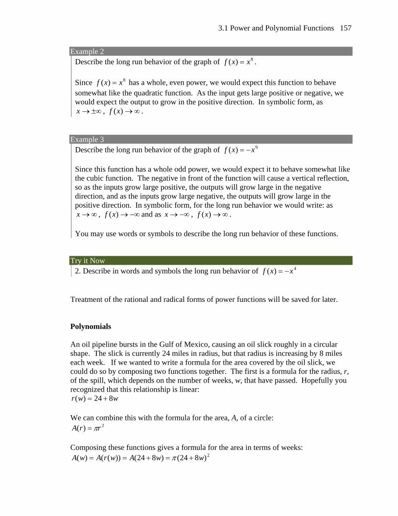
2. Describe in words and symbols the long run behavior of 4)( xxf Treatment of the rational and radical forms of power functions will be saved for later. Polynomials An oil pipeline bursts in the Gulf of Mexico, causing an oil slick roughly in a circular shape. The slick is currently 24 miles in radius, but that radius is increasing by 8 miles each week. If we wanted to write a formula for the area covered by the oil slick, we could do so by composing two functions together. The first is a formula for the radius, r, of the spill, which depends on the number of weeks, w, that have passed. Hopefully you recognized that this relationship is linear:

wwr 824)( We can combine this with the formula for the area, A, of a circle:

2)( rrA Composing these functions gives a formula for the area in terms of weeks:

2)824()824())(()( wwAwrAwA

Chapter 3

158

Multiplying this out gives the formula

264384576)( wwwA This formula is an example of a polynomial. A polynomial is simply the sum of terms consisting of transformed power functions with positive whole number powers. Terminology of Polynomial Functions

A polynomial is function of the form nn xaxaxaaxf 2

210)(

Each of the ai constants are called coefficients and can be positive, negative, whole numbers, decimals, or fractions. A term of the polynomial is any one piece of the sum, any i

i xa . Each individual term is

a transformed power function The degree of the polynomial is the highest power of the variable that occurs in the polynomial. The leading term is the term containing the highest power of the variable; the term with the highest degree. The leading coefficient is the coefficient on the leading term. Because of the definition of the leading term we often rearrange polynomials so that the powers are descending and the parts are easier to determine.

012

2.....)( axaxaxaxf nn

Example 4

Identify the degree, leading term, and leading coefficient of these polynomials: 32 423)( xxxf

ttttg 725)( 35

26)( 3 ppph For the function f(x), the degree is 3, the highest power on x. The leading term is the term containing that power, 34x . The leading coefficient is the coefficient of that term, -4. For g(t), the degree is 5, the leading term is 55t , and the leading coefficient is 5. For h(p), the degree is 3, the leading term is 3p , so the leading coefficient is -1.


159

Long Run Behavior of Polynomials For any polynomial, the long run behavior of the polynomial will match the long run behavior of the leading term.

Example 5

What can we determine about the long run behavior and degree of the equation for the polynomial graphed here?

Since the graph grows large and positive as the inputs grow large and positive, we describe the long run behavior symbolically by writing: as x , )(xf , and as

x , )(xf . In words we could say that as x values approach infinity, the function values approach infinity, and as x values approach negative infinity the function values approach negative infinity. We can tell this graph has the shape of an odd degree power function which has not been reflected, so the degree of the polynomial creating this graph must be odd.

Try it Now

3. Given the function )5)(1)(2(2.0)( xxxxf use your algebra skills write the function in polynomial form and determine the leading term, degree, and long run behavior of the function.

Short Run Behavior Characteristics of the graph such as vertical and horizontal intercepts and the places the graph changes direction are part of the short run behavior of the polynomial. Like with all functions, the vertical intercept is where the graph crosses the vertical axis, and occurs when the input value is zero. Since a polynomial is a function, there can only be one vertical intercept, which occurs at 0a , or the point ),0( 0a . The horizontal

intercepts occur at the input values that correspond with an output value of zero. It is possible to have more than one horizontal intercept.

Chapter 3

160

Example 6 Given the polynomial function )4)(1)(2()( xxxxf , given in factored form for your convenience, determine the vertical and horizontal intercepts. The vertical intercept occurs when the input is zero.

8)40)(10)(20()0( f . The graph crosses the vertical axis at the point (0, 8) The horizontal intercepts occur when the output is zero.

)4)(1)(2(0 xxx when x = 2, -1, or 4 The graph crosses the horizontal axis at the points (2, 0), (-1, 0), and (4, 0)

Notice that the polynomial in the previous example, which would be degree three if multiplied out, had three horizontal intercepts and two turning points - places where the graph changes direction. We will make a general statement here without justification at this time – the reasons will become clear later in this chapter. Intercepts and Turning Points of Polynomials

A polynomial of degree n will have: At most n horizontal intercepts. An odd degree polynomial will always have at least one. At most n-1 turning points

Example 7

What can we conclude about the graph of the polynomial shown here?

Based on the long run behavior, with the graph becoming large positive on both ends of the graph, we can determine that this is the graph of an even degree polynomial. The graph has 2 horizontal intercepts, suggesting a degree of 2 or greater, and 3 turning points, suggesting a degree of 4 or greater. Based on this, it would be reasonable to conclude that the degree is even and at least 4, so it is probably a fourth degree polynomial.


161

Try it Now 4. Given the function )5)(1)(2(2.0)( xxxxf determine the short run behavior.

Important Topics of this Section

Power Functions Polynomials Coefficients Leading coefficient Term Leading Term Degree of a polynomial Long run behavior Short run behavior

Try it Now Answers

1. (0, 0) and (1, 1) are common to all power functions 2. As x approaches positive and negative infinity, f(x) approaches negative infinity: as

x , )(xf because of the vertical flip.

3. The leading term is 32.0 x , so it is a degree 3 polynomial, as x approaches infinity (or gets very large in the positive direction) f(x) approaches infinity, and as x approaches negative infinity (or gets very large in the negative direction) f(x) approaches negative infinity. (Basically the long run behavior is the same as the cubic function) 4. Horizontal intercepts are (2, 0) (-1, 0) and (5, 0), the vertical intercept is (0, 2) and there are 2 turns in the graph.

Chapter 3

162

Section 3.1 Exercises Find the long run behavior of each function as x and x 1. 4f x x 2. 6f x x 3. 3f x x 4. 5f x x

5. 2f x x 6. 4f x x 7. 7f x x 8. 9f x x

Find the degree and leading coefficient of each polynomial 9. 74x 10. 65x 11. 25 x 12. 36 3 4x x 13. 4 22 3 1 x x x 14. 5 4 26 2 3x x x 15. 2 3 4 (3 1)x x x 16. 3 1 1 (4 3)x x x

Find the long run behavior of each function as x and x 17. 4 22 3 1 x x x 18. 5 4 26 2 3x x x 19. 23 2x x 20. 3 22 3x x x 21. What is the maximum number of x-intercepts and turning points for a polynomial of degree 5? 22. What is the maximum number of x-intercepts and turning points for a polynomial of degree 8? What is the least possible degree of each graph?

23. 24. 25. 26.

27. 28. 29. 30. Find the vertical and horizontal intercepts of each function 31. 2 1 2 ( 3)f t t t t 32. 3 1 4 ( 5)f x x x x

33. 2 3 1 (2 1)g n n n 34. 3 4 (4 3)k u n n

3.2 Quadratic Functions

163

Section 3.2 Quadratic Functions In this section, we will explore the family of 2nd degree polynomials, the quadratic functions. While they share many characteristics of polynomials in general, the calculations involved in working with quadratics is typically a little simpler, which makes them a good place to start our exploration of short run behavior. In addition, quadratics commonly arise from problems involving area and projectile motion, providing some interesting applications. Example 1

A backyard farmer wants to enclose a rectangular space for a new garden. She has purchased 80 feet of wire fencing to enclose 3 sides, and will put the 4th side against the backyard fence. Find a formula for the area of the fence if the sides of fencing perpendicular to the existing fence have length L. In a scenario like this involving geometry, it is often helpful to draw a picture. It might also be helpful to introduce a temporary variable, W, to represent the side of fencing parallel to the 4th side or backyard fence. Since we know we only have 80 feet of fence available, we know that

80 LWL , or more simply, 802 WL This allows us to represent the width, W, in terms of L: LW 280 Now we are ready to write an equation for the area the fence encloses. We know the area of a rectangle is length multiplied by width, so

)280( LLLWA 2280)( LLLA

This formula represents the area of the fence in terms of the variable length L. Short run Behavior: Vertex We now explore the interesting features of the graphs of quadratics. In addition to intercepts, quadratics have an interesting feature where they change direction, called the vertex. You probably noticed that all quadratics are related to transformations of the basic quadratic function 2)( xxf .

Backyard

Garden

W

L

Chapter 3

164

Example 2 Write an equation for the quadratic graphed below as a transformation of 2)( xxf , then expand the formula and simplify terms to write the equation in standard polynomial form.

We can see the graph is the basic quadratic shifted to the left 2 and down 3, giving a formula in the form 3)2()( 2 xaxg . By plugging in a clear point such as (0,-1) we can solve for the stretch factor:

2

1

42

3)20(1 2

a

a

a

Written as a transformation, the equation for this formula is 3)2(2

1)( 2 xxg . To

write this in standard polynomial form, we can expand the formula and simplify terms:

122

1)(

3222

1)(

3)44(2

1)(

3)2)(2(2

1)(

3)2(2

1)(

2

2

2

2

xxxg

xxxg

xxxg

xxxg

xxg

Notice that the horizontal and vertical shifts of the basic quadratic determine the location of the vertex of the parabola; the vertex is unaffected by stretches and compressions.


165

Try it Now 1. A coordinate grid has been superimposed

over the quadratic path of a basketball1. Find an equation for the path of the ball. Does he make the basket?

Forms of Quadratic Functions

The standard form of a quadratic is cbxaxxf 2)(

The transformation form of a quadratic is khxaxf 2)()( The vertex of the quadratic is located at (h, k) Because the vertex can also be seen in this format it is often called vertex form as well

In the previous example, we saw that it is possible to rewrite a quadratic in transformed form into standard form by expanding the formula. It would be useful to reverse this process, since the transformation form reveals the vertex. Expanding out the general transformation form of a quadratic gives:

kahahxaxkhxhxaxf

khxhxakhxaxf

2222

2

2)2()(

))(()()(

This should be equal to the standard form of the quadratic:

cbxaxkahahxax 222 2 The second degree terms are already equal. For the linear terms to be equal, the coefficients must be equal:

bah 2 , so a

bh

2

This provides us a method to determine the horizontal shift of the quadratic from the standard form. We could likewise set the constant terms equal to find:

ckah 2 , so a

bc

a

bac

a

bacahck

442

2

2

222

In practice, though, it is usually easier to remember that k is the output value of the function when the input is h, so )(hfk .

1 From http://blog.mrmeyer.com/?p=4778, © Dan Meyer, CC-BY

Chapter 3

166

Finding Vertex of a Quadratic For a quadratic given in standard form, the vertex (h, k) is located at:

a

bh

2 , )(

2hf

a

bfk

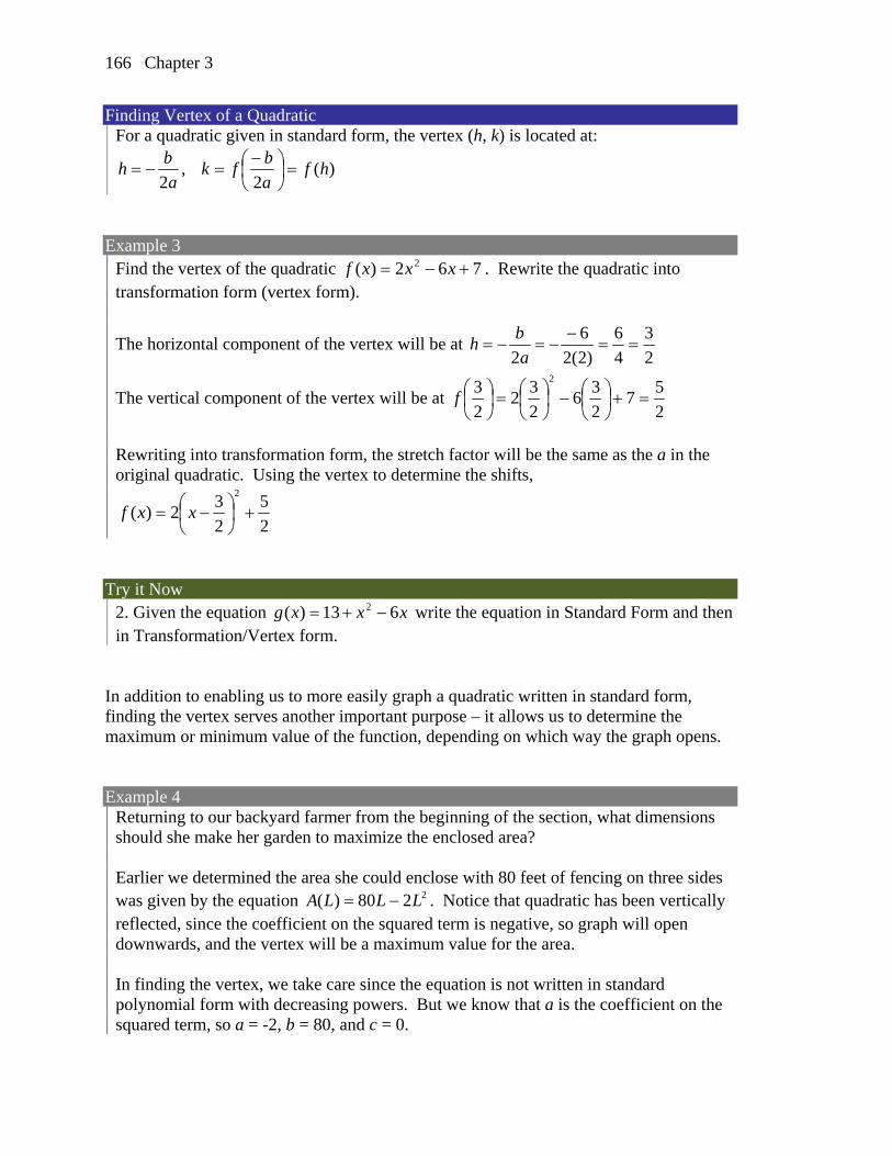
Example 3

Find the vertex of the quadratic 762)( 2 xxxf . Rewrite the quadratic into transformation form (vertex form).

The horizontal component of the vertex will be at 2

3

4

6

)2(2

6

2

a

bh

The vertical component of the vertex will be at 2

57

2

36

2

32

2

32

f

Rewriting into transformation form, the stretch factor will be the same as the a in the original quadratic. Using the vertex to determine the shifts,

2

5

2

32)(

2

xxf

Try it Now

2. Given the equation xxxg 613)( 2 write the equation in Standard Form and then in Transformation/Vertex form.

In addition to enabling us to more easily graph a quadratic written in standard form, finding the vertex serves another important purpose – it allows us to determine the maximum or minimum value of the function, depending on which way the graph opens. Example 4

Returning to our backyard farmer from the beginning of the section, what dimensions should she make her garden to maximize the enclosed area? Earlier we determined the area she could enclose with 80 feet of fencing on three sides was given by the equation 2280)( LLLA . Notice that quadratic has been vertically reflected, since the coefficient on the squared term is negative, so graph will open downwards, and the vertex will be a maximum value for the area. In finding the vertex, we take care since the equation is not written in standard polynomial form with decreasing powers. But we know that a is the coefficient on the squared term, so a = -2, b = 80, and c = 0.


167

Finding the vertex:

20)2(2

80

h , 800)20(2)20(80)20( 2 Ak

The maximum value of the function is an area of 800 square feet, which occurs when L = 20 feet. When the shorter sides are 20 feet, that leaves 40 feet of fencing for the longer side. To maximize the area, she should enclose the garden so the two shorter sides have length 20 feet, and the longer side parallel to the existing fence has length 40 feet.

Example 5

A local newspaper currently has 84,000 subscribers, at a quarterly cost of $30. Market research has suggested that if they raised the price to $32, they would lose 5,000 subscribers. Assuming that subscriptions are linearly related to the cost, what price should the newspaper charge for a quarterly subscription to maximize their revenue? Revenue is the amount of money a company brings in. In this case, the revenue can be found by multiplying the cost per subscription times the number of subscribers. We can introduce variables, C for cost per subscription and S for the number subscribers, giving us the equation Revenue = CS Since the number of subscribers changes with the price, we need to find a relationship between the variables. We know that currently S = 84,000 and C = 30, and that if they raise the price to $32 they would lose 5,000 subscribers, giving a second pair of values, C = 32 and S = 79,000. From this we can find a linear equation relating the two quantities. Treating C as the input and S as the output, the equation will have form

bmCS . The slope will be

500,22

000,5

3032

000,84000,79

m

This tells us the paper will lose 2,500 subscribers for each dollar they raise the price. We can then solve for the vertical intercept

bCS 2500 Plug in the point S = 85,000 and C = 30 b )30(2500000,84 Solve for b

000,159b This gives us the linear equation 000,159500,2 CS relating cost and subscribers. We now return to our revenue equation.

CSRevenue Substituting the equation for S from above )000,159500,2(Revenue CC Expanding

CC 000,159500,2Revenue 2

Chapter 3

168

We now have a quadratic equation for revenue as a function of the subscription cost. To find the cost that will maximize revenue for the newspaper, we can find the vertex:

8.31)500,2(2

000,159

h

The model tells us that the maximum revenue will occur if the newspaper charges $31.80 for a subscription. To find what the maximum revenue is, we can evaluate the revenue equation: Maximum Revenue = )8.31(000,159)8.31(500,2 2 $2,528,100

Short run Behavior: Intercepts As with any function, we can find the vertical intercepts of a quadratic by evaluating the function at an input of zero, and we can find the horizontal intercepts by solving for when the output will be zero. Notice that depending upon the location of the graph, we might have zero, one, or two horizontal intercepts.

zero horizontal intercepts one horizontal intercept two horizontal intercepts

Example 6

Find the vertical and horizontal intercepts of the quadratic 253)( 2 xxxf We can find the vertical intercept by evaluating the function at an input of zero:

22)0(5)0(3)0( 2 f Vertical intercept at (0,-2) For the horizontal intercepts, we solve for when the output will be zero

2530 2 xx In this case, the quadratic can be factored, providing the simplest method for solution

)2)(13(0 xx

3

1

130

x

x or

2

20

x

x Horizontal intercepts at

0,3

1 and (-2,0)


169

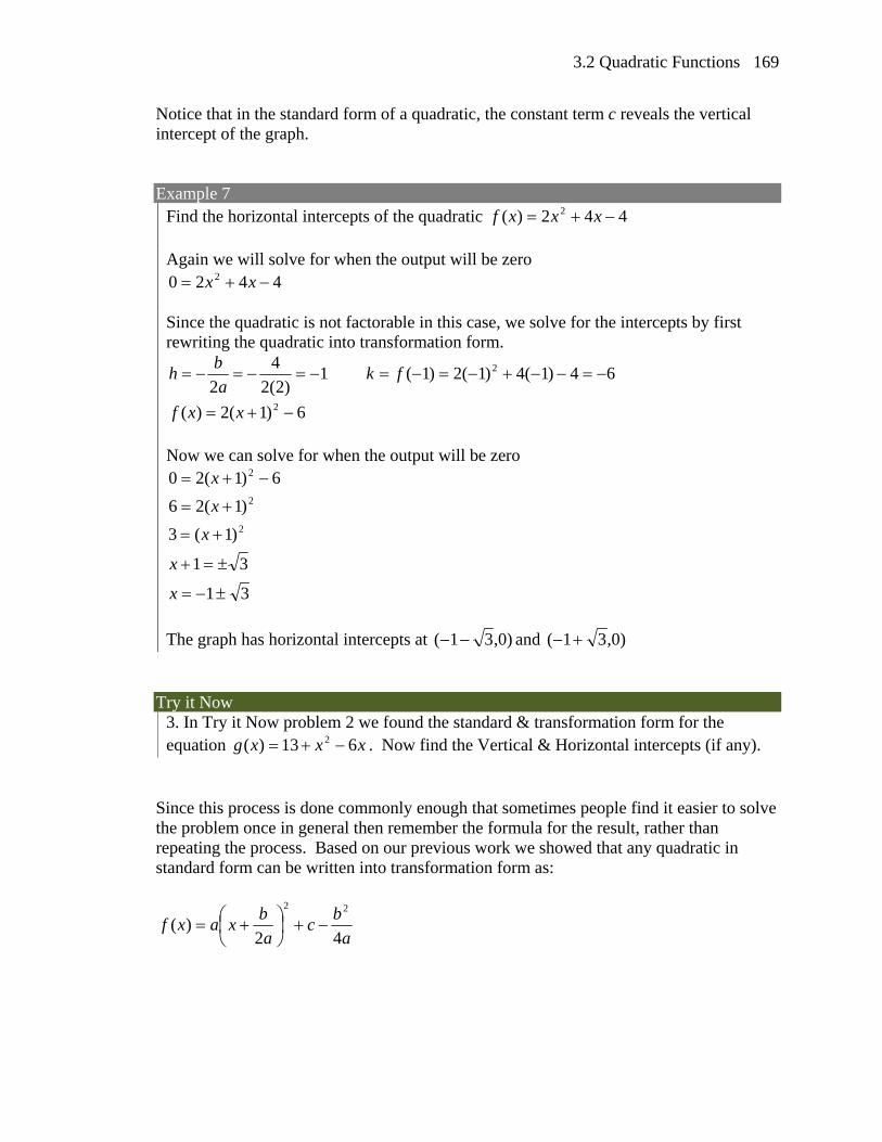
Notice that in the standard form of a quadratic, the constant term c reveals the vertical intercept of the graph. Example 7

Find the horizontal intercepts of the quadratic 442)( 2 xxxf Again we will solve for when the output will be zero

4420 2 xx Since the quadratic is not factorable in this case, we solve for the intercepts by first rewriting the quadratic into transformation form.

1)2(2

4

2

a

bh 64)1(4)1(2)1( 2 fk

6)1(2)( 2 xxf Now we can solve for when the output will be zero

31

31

)1(3

)1(26

6)1(20

2

2

2

x

x

x

x

x

The graph has horizontal intercepts at )0,31( and )0,31( Try it Now

3. In Try it Now problem 2 we found the standard & transformation form for the equation xxxg 613)( 2 . Now find the Vertical & Horizontal intercepts (if any).

Since this process is done commonly enough that sometimes people find it easier to solve the problem once in general then remember the formula for the result, rather than repeating the process. Based on our previous work we showed that any quadratic in standard form can be written into transformation form as:

a

bc

a

bxaxf

42)(

22

Chapter 3

170

Solving for the horizontal intercepts using this general equation gives:

a

bc

a

bxa

420

22

start to solve for x by moving the constants to the other side

22

24

a

bxac

a

b divide both sides by a

2

2

2

24

a

bx

a

c

a

b find a common denominator to combine fractions

2

22

2

24

4

4

a

bx

a

ac

a

b combine the fractions on the left side of the equation

2

2

2

24

4

a

bx

a

acb take the square root of both sides

a

bx

a

acb

24

42

2

subtract b/2a from both sides

xa

acb

a

b

2

4

2

2

combining the fractions

a

acbbx

2

42 Notice that this can yield two different answers for x

Quadratic Formula

For a quadratic given in standard form, the quadratic formula gives the horizontal intercepts of the graph of the quadratic.

a

acbbx

2

42

Example 8

A ball is thrown upwards from the top of a 40 foot high building at a speed of 80 feet per second. The ball’s height above ground can be modeled by the equation

408016)( 2 ttth . What is the maximum height of the ball? When does the ball hit the ground? To find the maximum height of the ball, we would need to know the vertex of the quadratic.

2

5

32

80

)16(2

80

h , 14040

2

580

2

516

2

52

hk

The ball reaches a maximum height of 140 feet after 2.5 seconds


171

To find when the ball hits the ground, we need to determine when the height is zero – when h(t) = 0. While we could do this using the transformation form of the quadratic, we can also use the quadratic formula:

32

896080

)16(2

)40)(16(48080 2

t

Since the square root does not evaluate to a whole number, we can use a calculator to approximate the values of the solutions:

458.532

896080

t or 458.032

896080

t

The second answer is outside the reasonable domain of our model, so we conclude the ball will hit the ground after about 5.458 seconds.

Try it Now

4. For these two equations determine if the vertex will be a maximum value or a minimum value. a. 78)( 2 xxxg

b. 2)3(3)( 2 xxg Important Topics of this Section

Quadratic functions Standard form Transformation form/Vertex form Vertex as a maximum / Vertex as a minimum Short run behavior Vertex / Horizontal & Vertical intercepts Quadratic formula

Try it Now Answers

1. The path passes through the origin with vertex at (-4, 7). 27

( ) ( 4) 716

h x x . To make the shot, h(-7.5) would

need to be about 4. ( 7.5) 1.64h ; he doesn’t make it. 2. 136)( 2 xxxg in Standard form; 4)3()( 2 xxg in Transformation form 3. Vertical intercept at (0, 13), NO horizontal intercepts. 4. a. Vertex is a minimum value b. Vertex is a maximum value

Chapter 3

172

Section 3.2 Exercises Write an equation for the quadratic graphed

1. 2.

3. 4.

5. 6. For each of the follow quadratics, find a) the vertex, b) the vertical intercept, and c) the horizontal intercepts. 7. 22 10 12y x x x 8. 23 6 9z p x x

9. 22 10 4f x x x 10. 22 14 12g x x x

11. 24 6 1h t t t 12. 22 4 15 k t x x

Rewrite the quadratic into vertex form 13. 2 12 32f x x x 14. 2 2 3g x x x

15. 22 8 10h x x x 16. 23 6 9k x x x


173

17. Find the values of b and c so 28f x x bx c has vertex 2, 7

18. Find the values of b and c so 26f x x bx c has vertex (7, 9)

Write an equation for a quadratic with the given features 19. x-intercepts (-3, 0) and (1, 0), and y intercept (0, 2) 20. x-intercepts (2, 0) and (-5, 0), and y intercept (0, 3) 21. x-intercepts (2, 0) and (5, 0), and y intercept (0, 6) 22. x-intercepts (1, 0) and (3, 0), and y intercept (0, 4) 23. Vertex at (4, 0), and y intercept (0, -4) 24. Vertex at (5, 6), and y intercept (0, -1) 25. Vertex at (-3, 2), and passing through (3, -2) 26. Vertex at (1, -3), and passing through (-2, 3)

27. A rocket is launched in the air. Its height, in meters above sea level, as a function of

time is given by 24.9 229 234h t t t .

a. From what height was the rocket launched? b. How high above sea level does the rocket get at its peak? c. Assuming the rocket will splash down in the ocean, at what time does

splashdown occur?

28. A ball is thrown in the air from the top of a building. Its height, in meters above

ground, as a function of time is given by 24.9 24 8h t t t .

a. From what height was the ball thrown? b. How high above ground does the ball get at its peak? c. When does the ball hit the ground?

29. The height of a ball thrown in the air is given by 216 3

12h x x x , where x is

the horizontal distance in feet from the point at which the ball is thrown. a. How high is the ball when it was thrown? b. What is the maximum height of the ball? c. How far from the thrower does the ball strike the ground?

30. A javelin is thrown in the air. Its height is given by 218 6

20h x x x , where x

is the horizontal distance in feet from the point at which the javelin is thrown. a. How high is the javelin when it was thrown? b. What is the maximum height of the javelin? c. How far from the thrower does the javelin strike the ground?

Chapter 3

174

31. A box with a square base and no top is to be made from a square piece of cardboard by cutting 6 in. squares from each corner and folding up the sides. The box is to hold 1000 in3. How big a piece of cardboard is needed?

32. A box with a square base and no top is to be made from a square piece of cardboard by cutting 4 in. squares from each corner and folding up the sides. The box is to hold 2700 in3. How big a piece of cardboard is needed?

33. A farmer wishes to enclose two pens with fencing, as shown. If the farmer has 500 feet of fencing to work with, what dimensions will maximize the area enclosed?

34. A farmer wishes to enclose three pens with fencing, as shown. If the farmer has 700 feet of fencing to work with, what dimensions will maximize the area enclosed?

35. You have a wire that is 56 cm long. You wish to cut it into two pieces. One piece will

be bent into the shape of a square. The other piece will be bent into the shape of a circle. Let A represent the total area of the square and the circle. What is the circumference of the circle when A is a minimum?

36. You have a wire that is 71 cm long. You wish to cut it into two pieces. One piece will be bent into the shape of a right triangle with base equal to height. The other piece will be bent into the shape of a circle. Let A represent the total area of the triangle and the circle. What is the circumference of the circle when A is a minimum?

37. A soccer stadium holds 62000 spectators. With a ticket price of $11 the average attendance has been 26,000. When the price dropped to $9, the average attendance rose to 31,000. Assuming that attendance is linearly related to ticket price, what ticket price would maximize revenue?

38. A farmer finds that if she plants 75 trees per acre, each tree will yield 20 bushels of fruit. She estimates that for each additional tree planted per acre, the yield of each tree will decrease by 3 bushels. How many trees should she plant per acre to maximize her harvest?


175

39. A hot air balloon takes off from the edge of a mountain lake. Impose a coordinate system as pictured and assume that the path of the balloon follows the graph of

2245

2500f x x x . The land rises

at a constant incline from the lake at the rate of 2 vertical feet for each 20 horizontal feet. [UW]

a. What is the maximum height of the balloon above plateau level? b. What is the maximum height of the balloon above ground level? c. Where does the balloon land on the ground? d. Where is the balloon 50 feet above the ground?

40. A hot air balloon takes off from

the edge of a plateau. Impose a coordinate system as pictured below and assume that the path the balloon follows is the graph of the quadratic function

24 4

2500 5f x x x . The

land drops at a constant incline from the plateau at the rate of 1 vertical foot for each 5 horizontal feet. [UW]

a. What is the maximum height of the balloon above plateau level? b. What is the maximum height of the balloon above ground level? c. Where does the balloon land on the ground? d. Where is the balloon 50 feet above the ground?

Chapter 3

176

Section 3.3 Graphs of Polynomial Functions In the previous section we explored the short run behavior of quadratics, a special case of polynomials. In this section we will explore the short run behavior of polynomials in general. Short run Behavior: Intercepts As with any function, the vertical intercept can be found by evaluating the function at an input of zero. Since this is evaluation, it is relatively easy to do it for any degree polynomial. To find horizontal intercepts, we need to solve for when the output will be zero. For general polynomials, this can be a challenging prospect. While quadratics can be solved using the relatively simple quadratic formula, the corresponding formulas for cubic and 4th degree polynomials are not simple enough to remember, and formulas do not exist for general higher degree polynomials. Consequently, we will limit ourselves to three cases:

1) The polynomial can be factored using known methods: greatest common factor and trinomial factoring.

2) The polynomial is given in factored form 3) Technology is used to determine the intercepts

Example 1

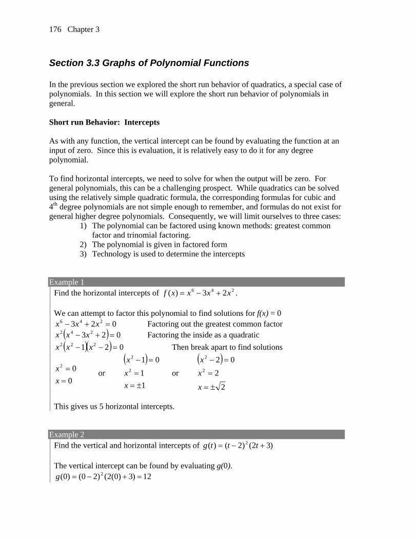
Find the horizontal intercepts of 246 23)( xxxxf . We can attempt to factor this polynomial to find solutions for f(x) = 0

023 246 xxx Factoring out the greatest common factor 023 242 xxx Factoring the inside as a quadratic

021 222 xxx Then break apart to find solutions

0

02

x

x or

1

1

012

2

x

x

x

or

2

2

022

2

x

x

x

This gives us 5 horizontal intercepts.

Example 2

Find the vertical and horizontal intercepts of )32()2()( 2 tttg The vertical intercept can be found by evaluating g(0).

12)3)0(2()20()0( 2 g

3.3 Graphs of Polynomial Functions

177

The horizontal intercepts can be found by solving g(t) = 0 0)32()2( 2 tt Since this is already factored, we can break it apart:

2

02

0)2( 2

t

t

t

or

2

3

0)32(

t

t

Example 3

Find the horizontal intercepts of 64)( 23 tttth

Since this polynomial is not in factored form, has no common factors, and does not appear to be factorable using techniques we know, we can turn to technology to find the intercepts. Graphing this function, it appears there are horizontal intercepts at x = -3, -2, and 1

Try it Now

1. Find the vertical and horizontal intercepts of the function 24 4)( tttf Graphical Behavior at Intercepts If we graph the function

32 )1()2)(3()( xxxxf , notice that the behavior at each of the horizontal intercepts is different. At the horizontal intercept x = -3, coming from the )3( x factor of the polynomial, the graph passes directly through the horizontal intercept. The factor is linear (has a power of 1), so the behavior near the intercept is like that of a line - it passes directly through the intercept. We call this a single zero, since the zero is formed from a single factor of the function. At the horizontal intercept x = 2, coming from the 2)2( x factor of the polynomial, the graph touches the axis at the intercept and changes direction. The factor is quadratic (degree 2), so the behavior near the intercept is like that of a quadratic – it bounces off of

Chapter 3

178

the horizontal axis at the intercept. Since )2)(2()2( 2 xxx , the factor is repeated twice, so we call this a double zero. At the horizontal intercept x = -1, coming from the 3)1( x factor of the polynomial, the graph passes through the axis at the intercept, but flattens out a bit first. This factor is cubic (degree 3), so the behavior near the intercept is like that of a cubic, with the same “S” type shape near the intercept that the toolkit 3x has. We call this a triple zero. By utilizing these behaviors, we can sketch a reasonable graph of a factored polynomial function without needing technology. Graphical Behavior of Polynomials at Horizontal Intercepts

If a polynomial contains a factor of the form phx )( , the behavior near the horizontal intercept h is determined by the power on the factor. p = 1 p = 2 p = 3

Single zero Double zero Triple zero For higher even powers 4,6,8 etc… the graph will still bounce off of the graph but the graph will appear flatter with increasing even power as it approaches and leaves the axis. For higher odd powers, 5,7,9 etc… the graph will still pass through the graph but the graph will appear flatter with increasing odd power as it approaches and leaves the axis.

Example 4

Sketch a graph of )5()3(2)( 2 xxxf This graph has two horizontal intercepts. At x = -3, the factor is squared, indicating the graph will bounce at this horizontal intercept. At x = 5, the factor is not squared, indicating the graph will pass through the axis at this intercept. Additionally, we can see the leading term, if this polynomial were multiplied out, would be 32x , so the long-run behavior is that of a vertically reflected cubic, with the outputs decreasing as the inputs get large positive, and the inputs increasing as the inputs get large negative.


179

To sketch this we consider the following: As x the function )(xf so we know the graph starts in the 2nd quadrant and is decreasing toward the horizontal axis. At (-3, 0) the graph bounces off of the horizontal axis and so the function must start increasing. At (0, 90) the graph crosses the vertical axis at the vertical intercept Somewhere after this point the graph must turn back down / or start decreasing toward the horizontal axis since the graph passes through the next intercept at (5,0) As x the function )(xf so we know the graph continues to decrease and we can stop drawing the graph in the 4th quadrant. Using technology we see that the resulting graph will look like:

Solving Polynomial Inequalities One application of our ability to find intercepts and sketch a graph of polynomials is the ability to solve polynomial inequalities. It is a very common question to ask when a function will be positive and negative. We can solve polynomial inequalities by either utilizing the graph, or by using test values. Example 5

Solve 0)4()1)(3( 2 xxx As with all inequalities, we start by solving the equality 0)4()1)(3( 2 xxx , which has solutions at x = -3, -1, and 4. We know the function can only change from positive to negative at these values, so these divide the inputs into 4 intervals.

Chapter 3

180

We could choose a test value in each interval and evaluate the function )4()1)(3()( 2 xxxxf at each test value to determine if the function is positive or

negative in that interval

On a number line this would look like:

From our test values, we can determine this function is positive when x < -3 or x > 4, or in interval notation, ),4()3,(

We could have also determined on which intervals the function was positive by sketching a graph of the function. We illustrate that technique in the next example Example 6

Find the domain of the function 256)( tttv A square root only is defined when the quantity we are taking the square root of is zero or greater. Thus, the domain of this function will be when 056 2 tt . Again we start by solving the equality 056 2 tt . While we could use the quadratic formula, this equation factors nicely to 0)1)(6( tt , giving horizontal intercepts t = 1 and t = -6. Sketching a graph of this quadratic will allow us to determine when it is positive:

From the graph we can see this function is positive for inputs between the intercepts. So 056 2 tt for 16 t , and this will be the domain of the v(t) function.

Interval Test x in interval f( test value) >0 or <0? x < -3 -4 72 > 0 -3 < x < -1 -2 -6 < 0 -1 < x .< 4 0 -12 < 0 x > 4 5 288 > 0

0 0 0 positive negative negative positive


181

Try it Now 2. Given the function xxxxg 6)( 23 use the methods that we have learned so far to find the vertical & horizontal intercepts, determine where the function is negative and positive, describe the long run behavior and sketch the graph without technology.

Writing Equations using Intercepts Since a polynomial function written in factored form will have a horizontal intercept where each factor is equal to zero, we can form an equation that will pass through a set of horizontal intercepts by introducing a corresponding set of factors. Factored Form of Polynomials

If a polynomial has horizontal intercepts at nxxxx ,,, 21 , then the polynomial can be

written in the factored form np

npp xxxxxxaxf )()()()( 21

21

where the powers pi on each factor can be determined by the behavior of the graph at the corresponding intercept, and the stretch factor a can be determined given a value of the function other than the horizontal intercept.

Example 7

Write an equation for the polynomial graphed here

This graph has three horizontal intercepts: x = -3, 2, and 5. At x = -3 and 5 the graph passes through the axis, suggesting the corresponding factors of the polynomial will be linear. At x = 2 the graph bounces at the intercept, suggesting the corresponding factor of the polynomial will be 2nd degree or quadratic. Together, this gives us:

)5()2)(3()( 2 xxxaxf To determine the stretch factor, we can utilize another point on the graph. Here, the vertical intercept appears to be (0,-2), so we can plug in those values to solve for a

Chapter 3

182

30

1

602

)50()20)(30(2 2

a

a

a

The graphed polynomial would have equation )5()2)(3(30

1)( 2 xxxxf

Try it Now

3. Given the graph, determine and write the equation for the graph in factored form.

Estimating Extrema With quadratics, we were able to algebraically find the maximum or minimum value of the function by finding the vertex. For general polynomials, finding these turning points is not possible without more advanced techniques from calculus. Even then, finding where extrema occur can still be algebraically challenging. For now, we will estimate the locations of turning points using technology to generate a graph. Example 8

An open-top box is to be constructed by cutting out squares from each corner of a 14cm by 20cm sheet of plastic then folding up the sides. Find the size of squares that should be cut out to maximize the volume enclosed by the box. We will start this problem by drawing a picture, labeling the width of the cut-out squares with a variable, w.

w

w


183

Notice that after a square is cut out from each end, it leaves (14-2w) cm by (20-2w) cm for the base of the box, and the box will be w cm tall. This gives the volume:

32 468280)220)(214()( wwwwwwwV Using technology to sketch a graph allows us to estimate the maximum value for the volume, restricted to reasonable values for w – values from 0 to 7.

From this graph, we can estimate the maximum value is around 340, and occurs when the squares are about 2.75cm square. To improve this estimate, we could use features of our technology if available, or simply change our window to zoom in on our graph.

From this zoomed-in view, we can refine our estimate for the max volume to about 339, when the squares are 2.7cm square.

Try it Now

4. Use technology to find the Maximum and Minimum values on the interval [-1, 4] of the equation )4()1()2(2.0)( 23 xxxxf .

Chapter 3

184

Important Topics of this Section Short Run Behavior Intercepts (Horizontal & Vertical) Methods to find Horizontal intercepts Factoring Methods Factored Forms Technology Graphical Behavior at intercepts Single, Double and Triple zeros (or power 1,2 & 3 behaviors) Solving polynomial inequalities using test values & graphing techniques Writing equations using intercepts Estimating extrema

Try it Now Answers

1. Vertical intercept (0, 0) Horizontal intercepts (0, 0), (-2, 0), (2, 0) 2. Vertical intercept (0, 0) Horizontal intercepts (-2, 0), (0, 0), (3, 0) The function is negative from ( , -2) and (0, 3) The function is positive from (-2, 0) and (3, ) The leading term is 3x so as x , )(xg and as x , )(xg

3. 3 21( ) ( 2) ( 1) ( 4)

8f x x x x

4. Approximately, (0, -6.5) minimum and approximately (3.5, 7) maximum.


185

Section 3.3 Exercises Find the C and t intercepts of each function 1. 2 4 1 ( 6)C t t t t 2. 3 2 3 ( 5)C t t t t

3. 24 2 ( 1)C t t t t 4. 2

2 3 1C t t t t

5. 4 3 22 8 6C t t t t 6. 4 3 24 12 40C t t t t

Use your calculator or other graphing technology to solve graphically for the zeros of the function 7. 3 27 4 30f x x x x 8. 3 26 28g x x x x

Find the long run behavior of each function as t and t

9. 3 33 5 3 ( 2)h t t t t 10. 2 3

2 3 1 ( 2)k t t t t

11. 22 1 3p t t t t 12. 3

4 2 1q t t t t

Sketch a graph of each equation

13. 23 ( 2)f x x x 14. 2

4 1g x x x

15. 3 21 3h x x x 16. 3 2

3 2k x x x

17. 2 1 ( 3)m x x x x 18. 3 2 ( 4)n x x x x

Solve each inequality

19. 23 2 0x x 20. 2

5 1 0x x

21. 1 2 3 0x x x 22. 4 3 6 0x x x

Find the domain of each function

23. 242 19 2f x x x 24. 228 17 3g x x x

25. 24 5h x x x 26. 22 7 3k x x x

27. 23 2n x x x 28. 2

1 ( 3)m x x x

29. 2

1

2 8p t

t t

30. 2

4

4 5q t

x x

Chapter 3

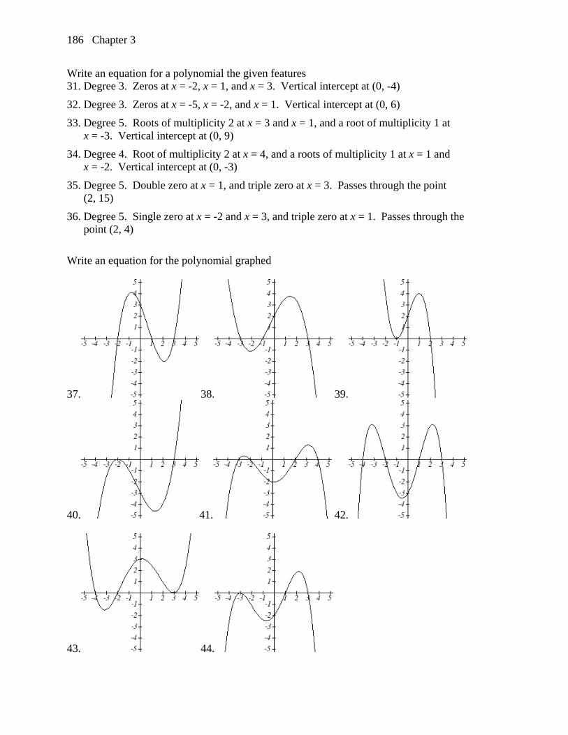
186

Write an equation for a polynomial the given features 31. Degree 3. Zeros at x = -2, x = 1, and x = 3. Vertical intercept at (0, -4)

32. Degree 3. Zeros at x = -5, x = -2, and x = 1. Vertical intercept at (0, 6)

33. Degree 5. Roots of multiplicity 2 at x = 3 and x = 1, and a root of multiplicity 1 at x = -3. Vertical intercept at (0, 9)

34. Degree 4. Root of multiplicity 2 at x = 4, and a roots of multiplicity 1 at x = 1 and x = -2. Vertical intercept at (0, -3)

35. Degree 5. Double zero at x = 1, and triple zero at x = 3. Passes through the point (2, 15)

36. Degree 5. Single zero at x = -2 and x = 3, and triple zero at x = 1. Passes through the point (2, 4)

Write an equation for the polynomial graphed

37. 38. 39.

40. 41. 42.

43. 44.


187

Write an equation for the polynomial graphed

45. 46.

47. 48.

49. 50. 51. A rectangle is inscribed with its base on the x axis and its upper corners on the

parabola 25y x . What are the dimensions of such a rectangle with the greatest

possible area?

52. A rectangle is inscribed with its base on the x axis and its upper corners on the curve 416y x . What are the dimensions of such a rectangle with the greatest possible

area?

Chapter 3

188

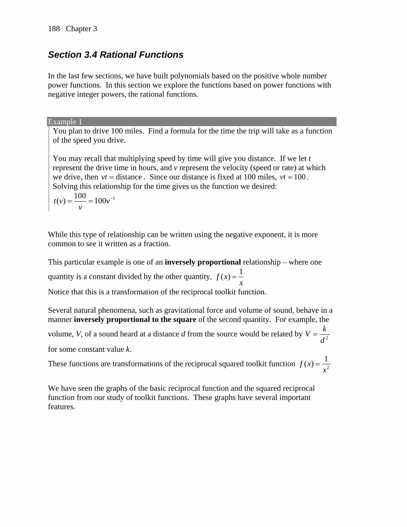
Section 3.4 Rational Functions In the last few sections, we have built polynomials based on the positive whole number power functions. In this section we explore the functions based on power functions with negative integer powers, the rational functions. Example 1

You plan to drive 100 miles. Find a formula for the time the trip will take as a function of the speed you drive. You may recall that multiplying speed by time will give you distance. If we let t represent the drive time in hours, and v represent the velocity (speed or rate) at which we drive, then distancevt . Since our distance is fixed at 100 miles, 100vt . Solving this relationship for the time gives us the function we desired:

1100100

)( vv

vt

While this type of relationship can be written using the negative exponent, it is more common to see it written as a fraction. This particular example is one of an inversely proportional relationship – where one

quantity is a constant divided by the other quantity. 1

( )f xx

Notice that this is a transformation of the reciprocal toolkit function. Several natural phenomena, such as gravitational force and volume of sound, behave in a manner inversely proportional to the square of the second quantity. For example, the

volume, V, of a sound heard at a distance d from the source would be related by 2d

kV

for some constant value k.

These functions are transformations of the reciprocal squared toolkit function 2

1( )f x

x

We have seen the graphs of the basic reciprocal function and the squared reciprocal function from our study of toolkit functions. These graphs have several important features.

3.4 Rational Functions

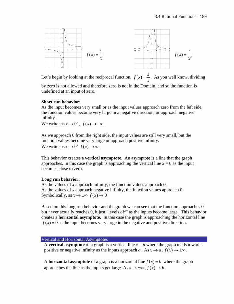
189

1( )f x

x

2

1( )f x

x

Let’s begin by looking at the reciprocal function, 1

( )f xx

. As you well know, dividing

by zero is not allowed and therefore zero is not in the Domain, and so the function is undefined at an input of zero. Short run behavior: As the input becomes very small or as the input values approach zero from the left side, the function values become very large in a negative direction, or approach negative infinity. We write: as 0x , )(xf . As we approach 0 from the right side, the input values are still very small, but the function values become very large or approach positive infinity. We write: as 0x )(xf . This behavior creates a vertical asymptote. An asymptote is a line that the graph approaches. In this case the graph is approaching the vertical line x = 0 as the input becomes close to zero. Long run behavior: As the values of x approach infinity, the function values approach 0. As the values of x approach negative infinity, the function values approach 0. Symbolically, as x 0)( xf Based on this long run behavior and the graph we can see that the function approaches 0 but never actually reaches 0, it just “levels off” as the inputs become large. This behavior creates a horizontal asymptote. In this case the graph is approaching the horizontal line

( ) 0f x as the input becomes very large in the negative and positive direction. Vertical and Horizontal Asymptotes

A vertical asymptote of a graph is a vertical line x = a where the graph tends towards positive or negative infinity as the inputs approach a. As ax , )(xf . A horizontal asymptote of a graph is a horizontal line ( )f x b where the graph approaches the line as the inputs get large. As x , bxf )( .

Chapter 3

190

Try it Now: 1. Use symbolic notation to describe the long run behavior and short run behavior for the reciprocal squared function.

Example 2

Sketch a graph of the reciprocal function shifted two units to the left and up three units. Identify the horizontal and vertical asymptotes of the graph, if any. Transforming the graph left 2 and up 3 would result in the equation

32

1)(

xxf , or equivalently by giving the terms a common denominator,

2

73)(

x

xxf

Shifting the toolkit function would give us this graph. Notice that this equation is undefined at x = -2, and the graph also is showing a vertical asymptote at x = -2. As 2x , ( )f x , and as

2x , ( )f x As the inputs grow large, the graph appears to be leveling off at ( ) 3f x , indicating a horizontal asymptote at ( ) 3f x . As x , 3)( xf . Notice that horizontal and vertical asymptotes shifted along with the function.

Try it Now

2. Sketch the graph and find the horizontal and vertical asymptotes of the reciprocal squared function that has been shifted right 3 units and down 4 units.

In the previous example, we shifted the function in a way that resulted in a function of the

form 2

73)(

x

xxf . This is an example of a general rational function.


191

Rational Function A rational function is a function that can be written as the ratio of two polynomials, p(x) and q(x).

qq

pp

xbxbxbb

xaxaxaa

xq

xpxf

2210

2210

)(

)()(

Example 3

A large mixing tank currently contains 100 gallons of water, into which 5 pounds of sugar have been mixed. A tap will open pouring 10 gallons per minute of water into the tank at the same time sugar is poured into the tank at a rate of 1 pound per minute. Find the concentration (pounds per gallon) of sugar in the tank after t minutes. Notice that the water in the tank is changing linearly, as is the amount of sugar in the tank. We can write an equation independently for each:

twater 10100 tsugar 15

The concentration, C, will be the ratio of pounds of sugar to gallons of water

t

ttC

10100

5)(

Finding Asymptotes and Intercepts Given a rational equation, as part of discovering the short run behavior we are interested in finding any vertical and horizontal asymptotes, as well as finding any vertical or horizontal intercepts as we have in the past. To find vertical asymptotes, we notice that the vertical asymptotes occurred when the denominator of the function was undefined. With few exceptions, a vertical asymptote will occur whenever the denominator is undefined. Example 4

Find the vertical asymptotes of the function 2

2

2

25)(

xx

xxk

To find the vertical asymptotes, we determine where this function will be undefined by setting the denominator equal to zero:

1,2

0)1)(2(

02 2

x

xx

xx

Chapter 3

192

This indicates two vertical asymptotes, which a look at a graph confirms.

The exception to this rule occurs when both the numerator and denominator of a rational function are zero. Example 5

Find the vertical asymptotes of the function 2

2( )

4

xk x

x

To find the vertical asymptotes, we determine where this function will be undefined by setting the denominator equal to zero:

2

2

4 0

4

2, 2

x

x

x

However, the numerator of this function is also equal to zero when x = 2. Because of this, the

function will still be undefined at 2, since 0

0 is

still undefined, but the graph will not have a vertical asymptote at x = 2. The graph of this function will have the vertical asymptote at x = -2, but at x = 2 the graph will have a hole; a single point where the graph is not defined, indicated by an open circle.

Vertical Asymptotes and Holes of Rational Functions

The vertical asymptotes of a rational function will occur where the denominator of the function is equal to zero and the numerator is not zero. A hole will occur in a rational function if an input causes both the numerator and denominator to both be zero.


193

To find horizontal asymptotes, we are interested in the behavior of the function as the input grows large, so we consider long run behavior of the numerator and denominator separately. Recall that a polynomial’s long run behavior will mirror that of the leading term. Likewise, a rational function’s long run behavior will mirror that of the ratio of the leading terms of the numerator and denominator functions. There are three distinct outcomes when this analysis is done: Case 1: The degree of the denominator > degree of the numerator

Example: 54

23)(

2

xx

xxf

In this case, the long run behavior is xx

xxf

33)(

2 . This tells us that as the inputs grow

large, this function will behave similarly to the function x

xf3

)( . As the inputs grow

large, the outputs will approach zero, resulting in a horizontal asymptote at ( ) 0f x . As x , 0)( xf Case 2: The degree of the denominator < degree of the numerator

Example: 5

23)(

2

x

xxf

In this case, the long run behavior is xx

xxf 3

3)(

2

. This tells us that as the inputs

grow large, this function will behave similarly to the function xxf 3)( . As the inputs grow large, the outputs will grow and not level off, so this graph has no horizontal asymptote. Instead, the graph will approach the slanted line xxf 3)( . As x , )(xf , respectively. Ultimately, if the numerator is larger than the denominator, the long run behavior of the graph will mimic the behavior of the reduced long run behavior fraction. As another

example if we had the function 5 23

( )3

x xf x

x

with long run behavior

45

33

)( xx

xxf , the long run behavior of the graph would look similar to that of an

even polynomial and as x , )(xf . Case 3: The degree of the denominator = degree of the numerator

Example: 54

23)(

2

2

xx

xxf

Chapter 3

194

In this case, the long run behavior is 33

)(2

2

x

xxf . This tells us that as the inputs

grow large, this function will behave the similarly to the function 3)( xf , which is a horizontal line. As x , 3)( xf , resulting in a horizontal asymptote at ( ) 3f x . Horizontal Asymptote of Rational Functions

The horizontal asymptote of a rational function can be determined by looking at the degrees of the numerator and denominator. Degree of denominator > degree of numerator: Horizontal asymptote at ( ) 0f x Degree of denominator < degree of numerator: No horizontal asymptote

Degree of denominator = degree of numerator: Horizontal asymptote at ratio of leading coefficients.

Example 6

In the sugar concentration problem from earlier, we created the equation

t

ttC

10100

5)(

.

Find the horizontal asymptote and interpret it in context of the scenario. Both the numerator and denominator are linear (degree 1), so since the degrees are equal, there will be a horizontal asymptote at the ratio of the leading coefficients. In the numerator, the leading term is t, with coefficient 1. In the denominator, the leading term is 10t, with coefficient 10. The horizontal asymptote will be at the ratio of these

values: As x , 10

1)( xf . This function will have a horizontal asymptote at

1( )

10f x .

This tells us that as the input gets large, the output values will approach 1/10. In context, this means that as more time goes by, the concentration of sugar in the tank will approach one tenth of a pound of sugar per gallon of water or 1/10 pounds per gallon.

Example 7

Find the horizontal and vertical asymptotes of the function

)5)(2)(1(

)3)(2()(

xxx

xxxf

The function will have vertical asymptotes when the denominator is zero causing the function to be undefined. The denominator will be zero at x = 1, -2, and 5, indicating vertical asymptotes at these values.


195

The numerator is degree 2, while the denominator is degree 3. Since the degree of the denominator is greater than the degree of the numerator, the denominator will grow faster than the numerator, causing the outputs to tend towards zero as the inputs get large, and so as x , 0)( xf . This function will have a horizontal asymptote at

( ) 0f x . Try it Now

3. Find the vertical and horizontal asymptotes of the function

)3)(2(

)12)(12()(

xx

xxxf

Intercepts As with all functions, a rational function will have a vertical intercept when the input is zero, if the function is defined at zero. It is possible for a rational function to not have a vertical intercept if the function is undefined at zero. Likewise, a rational function will have horizontal intercepts at the inputs that cause the output to be zero. It is possible there are no horizontal intercepts. Since a fraction is only equal to zero when the numerator is zero, horizontal intercepts will occur when the numerator of the rational function is equal to zero. Example 8

Find the intercepts of )5)(2)(1(

)3)(2()(

xxx

xxxf

We can find the vertical intercept by evaluating the function at zero

5

3

10

6

)50)(20)(10(

)30)(20()0(

f

The horizontal intercepts will occur when the function is equal to zero:

)5)(2)(1(

)3)(2(0

xxx

xx This is equivalent to when the numerator is zero

3,2

)3)(2(0

x

xx

Try it Now

4. Given the reciprocal squared function that is shifted right 3 units and down 4 units. Write this as a rational function and find the horizontal and vertical intercepts and the horizontal and vertical asymptotes.

Chapter 3

196

From the previous example, you probably noticed that the numerator of a rational function reveals the horizontal intercepts of the graph, while the denominator reveals the vertical asymptotes of the graph. As with polynomials, factors of the numerator may have powers. Happily, the effect on the shape of the graph at those intercepts is the same as we saw with polynomials. When factors of the denominator have power, the behavior at that intercept will mirror one of the two toolkit reciprocal functions.

We get this behavior when the degree of the factor in the denominator is odd. The distinguishing characteristic is that on one side of the vertical asymptote the graph increases, and on the other side the graph decreases. We get this behavior when the degree of the factor in the denominator is even. The distinguishing characteristic is that on both sides of the vertical asymptote the graph either increases or decreases.

For example, the graph of

)2()3(

)3()1()(

2

2

xx

xxxf is shown here.

At the horizontal intercept x = -1 corresponding to the 2)1( x factor of the numerator, the graph bounces at the intercept, consistent with the quadratic nature of the factor. At the horizontal intercept x = 3 corresponding to the )3( x factor of the numerator, the graph passes through the axis as we’d expect from a linear factor. At the vertical asymptote x = -3 corresponding to the 2)3( x factor of the denominator, the graph increases on both sides of the asymptote, consistent with the behavior of the

2

1

x toolkit.


197

At the vertical asymptote x = 2 corresponding to the )2( x factor of the denominator, the graph increases on the left side of the asymptote and decreases as the inputs approach

the asymptote from the right side, consistent with the behavior of the x

1 toolkit.

Example 9

Sketch a graph of 2

( 2)( 3)( )

( 1) ( 2)

x xf x

x x

We can start our sketch by finding intercepts and asymptotes. Evaluating the function at zero gives the vertical intercept:

2

(0 2)(0 3)(0) 3

(0 1) (0 2)f

Looking at when the numerator of the function is zero, we can determine the graph will have horizontal intercepts at x = -2 and x = 3. At each, the behavior will be linear, with the graph passing through the intercept. Looking at when the denominator of the function is zero, we can determine the graph will have vertical asymptotes at x = -1 and x = 2. Finally, the degree of denominator is larger than the degree of the numerator, telling us this graph has a horizontal asymptote at y = 0. To sketch the graph, we might start by plotting the three intercepts. Since the graph has no horizontal intercepts between the vertical asymptotes, and the vertical intercept is positive, we know the function must remain positive between the asymptotes, letting us fill in the middle portion of the graph. Since the factor associated with the vertical asymptote at x = -1 was squared, we know the graph will have the same behavior on both sides of the asymptote. Since the graph increases as the inputs approach the asymptote on the right, the graph will increase as the inputs approach the asymptote on the left as well. For the vertical asymptote at x = 2, the factor was not squared, so the graph will have opposite behavior on either side of the asymptote. After passing through the horizontal intercepts, the graph will then level off towards an output of zero, as indicated by the horizontal asymptote.

Chapter 3

198

Try it Now

5. Given the function )3()1(2

)2()2()(

2

2

xx

xxxf , use the characteristics of polynomials

and rational functions to describe the behavior and sketch the function . Since a rational function written in factored form will have a horizontal intercept where each factor of the numerator is equal to zero, we can form a numerator that will pass through a set of horizontal intercepts by introducing a corresponding set of factors. Likewise since the function will have a vertical asymptote where each factor of the denominator is equal to zero, we can form a denominator that will exhibit the vertical asymptotes by introducing a corresponding set of factors. Writing Rational Functions from Intercepts and Asymptotes

If a rational function has horizontal intercepts at nxxxx ,,, 21 , and vertical

asymptotes at mvvvx ,,, 21 then the function can be written in the form

n

n

qm

qq

pn

pp

vxvxvx

xxxxxxaxf

)()()(

)()()()(

21

21

21

21

where the powers pi or qi on each factor can be determined by the behavior of the graph at the corresponding intercept or asymptote, and the stretch factor a can be determined given a value of the function other than the horizontal intercept, or by the horizontal asymptote if it is nonzero.

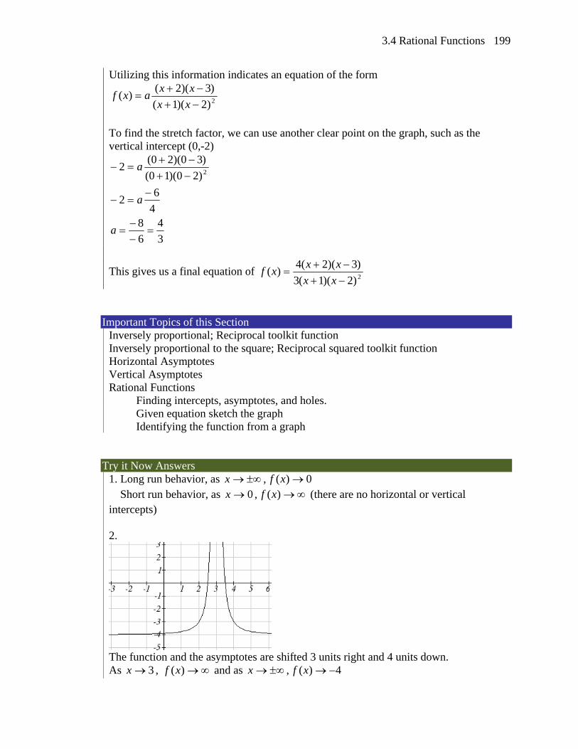
Example 10

Write an equation for the rational function graphed here. The graph appears to have horizontal intercepts at x = -2 and x = 3. At both, the graph passes through the intercept, suggesting linear factors. The graph has two vertical asymptotes. The one at x = -1 seems to exhibit the basic

behavior similar to x

1, with the graph increasing on one side and decreasing on the

other. The asymptote at x = 2 is exhibiting a behavior similar to 2

1

x, with the graph

decreasing on both sides of the asymptote.


199

Utilizing this information indicates an equation of the form

2)2)(1(

)3)(2()(

xx

xxaxf

To find the stretch factor, we can use another clear point on the graph, such as the vertical intercept (0,-2)

3

4

6

84

62

)20)(10(

)30)(20(2

2

a

a

a

This gives us a final equation of 2)2)(1(3

)3)(2(4)(

xx

xxxf

Important Topics of this Section

Inversely proportional; Reciprocal toolkit function Inversely proportional to the square; Reciprocal squared toolkit function Horizontal Asymptotes Vertical Asymptotes Rational Functions Finding intercepts, asymptotes, and holes. Given equation sketch the graph Identifying the function from a graph

Try it Now Answers

1. Long run behavior, as x , 0)( xf Short run behavior, as 0x , )(xf (there are no horizontal or vertical intercepts) 2.

The function and the asymptotes are shifted 3 units right and 4 units down. As 3x , )(xf and as x , 4)( xf

Chapter 3

200

3. Vertical asymptotes at x = 2 and x = -3; horizontal asymptote at y = 4 4. For the transformed reciprocal squared function, we find the rational form.

96

35244

)3)(3(

)96(41

)3(

)3(414

)3(

1)(

2

22

2

2

2

xx

xx

xx

xx

x

x

xxf

Since the numerator is the same degree as the denominator we know that as x , 4)( xf . 4)( xf is the horizontal asymptote. Next, we set the

denominator equal to zero to find the vertical asymptote at x = 3, because as 3x , )(xf . We set the numerator equal to 0 and find the horizontal intercepts are at

(2.5,0) and (3.5,0), then we evaluate at 0 and the vertical intercept is at

9

35,0

5. Horizontal asymptote at y = 1/2. Vertical asymptotes are at x = 1, and x = 3. Vertical intercept at (0, 4/3), Horizontal intercepts (2, 0) and (-2, 0) (-2, 0) is a double zero and the graph bounces off the axis at this point. (2, 0) is a single zero and crosses the axis at this point.


201

Section 3.4 Exercises Match each equation form with one of the graphs

1. x Af x

x B

2. 2

x Ag x

x B

3.

2

x Ah x

x B

4.

2

2

x Ak x

x B

A B C D For each function, find the x intercepts, the vertical intercept, the vertical asymptotes, and the horizontal asymptote. Use that information to sketch a graph.

5. 2 3

4

xp x

x

6. 5

3 1

xq x

x

7. 2

4

2s x

x

8.

2

5

1r x

x

9. 2

2

3 14 5

3 8 16

x xf x

x x

10.

2

2

2 7 15

3 14 15

x xg x

x

11. 2

2

2 3

1

x xa x

x

12.

2

2

6

4

x xb x

x

13. 22 1

4

x xh x

x

14.

22 3 20

5

x xk x

x

15. 2

3 2

3 4 4

4

x xn x

x x

16. 2

5

2 7 3

xm x

x x

17. 2

1 3 5

2 ( 4)

x x xw x

x x

18.

22 5

3 1 4

x xz x

x x x

Chapter 3

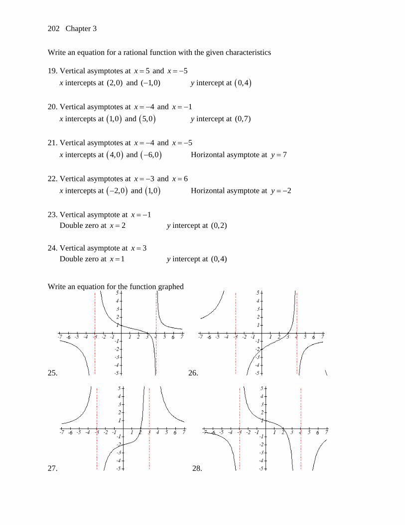
202

Write an equation for a rational function with the given characteristics 19. Vertical asymptotes at 5x and 5x

x intercepts at (2, 0) and ( 1, 0) y intercept at 0, 4

20. Vertical asymptotes at 4x and 1x

x intercepts at 1, 0 and 5, 0 y intercept at (0, 7)


x intercepts at 4, 0 and 6, 0 Horizontal asymptote at 7y


x intercepts at 2, 0 and 1, 0 Horizontal asymptote at 2y

23. Vertical asymptote at 1x

Double zero at 2x y intercept at (0, 2)

24. Vertical asymptote at 3x

Double zero at 1x y intercept at (0, 4)

Write an equation for the function graphed

25. 26. \

27. 28.


203


29. 30.

31. 32.

33. 34.

35. 36.

Chapter 3

204


37. 38. 39. A scientist has a beaker containing 20 mL of a solution containing 20% acid. To

dilute this, she adds pure water. a. Write an equation for the concentration in the beaker after adding n mL of

water b. Find the concentration if 10 mL of water is added c. How many mL of water must be added to obtain a 4% solution? d. What is the behavior as n , and what is the physical significance of this?

40. A scientist has a beaker containing 30 mL of a solution containing 3 grams of

potassium hydroxide. To this, she mixes a solution containing 8 milligrams per mL of potassium hydroxide.

a. Write an equation for the concentration in the tank after adding n mL of the second solution.

b. Find the concentration if 10 mL of the second solution is added c. How many mL of water must be added to obtain a 50 mg/mL solution? d. What is the behavior as n , and what is the physical significance of this?

41. Oscar is hunting magnetic fields with his gauss meter, a device for measuring the

strength and polarity of magnetic fields. The reading on the meter will increase as Oscar gets closer to a magnet. Oscar is in a long hallway at the end of which is a room containing an extremely strong magnet. When he is far down the hallway from the room, the meter reads a level of 0.2. He then walks down the hallway and enters the room. When he has gone 6 feet into the room, the meter reads 2.3. Eight feet into the room, the meter reads 4.4. [UW]

a. Give a rational model of form ax bm x

cx d

relating the meter reading ( )m x

to how many feet x Oscar has gone into the room. b. How far must he go for the meter to reach 10? 100? c. Considering your function from part (a) and the results of part (b), how far

into the room do you think the magnet is?


205

42. The more you study for a certain exam, the better your performance on it. If you study for 10 hours, your score will be 65%. If you study for 20 hours, your score will be 95%. You can get as close as you want to a perfect score just by studying long enough. Assume your percentage score, ( )p n , is a function of the number of hours, n,

that you study in the form ( )an b

p ncn d

. If you want a score of 80%, how long do

you need to study? [UW]

43. A street light is 10 feet North of a straight bike path that runs East-West. Olav is bicycling down the path at a rate of 15 MPH. At noon, Olav is 33 feet West of the point on the bike path closest to the street light. (See the picture). The relationship between the intensity C of light (in candlepower) and the distance d

(in feet) from the light source is given by 2

kC

d , where k is a constant depending on

the light source. [UW] a. From 20 feet away, the street light has an intensity of 1 candle. What is k? b. Find a function which gives the intensity of the light shining on Olav as a

function of time, in seconds. c. When will the light on Olav have maximum intensity? d. When will the intensity of the light be 2 candles?

Chapter 3

206

Section 3.5 Inverses and Radical Functions In this section, we will explore the inverses of polynomial and rational functions, and in particular the radical functions that arise from finding the inverses of quadratic functions. Example 1

A parabolic trough water runoff collector is built as shown below. Find the surface area of the water in the trough as a function of the depth of the water. Since it will be helpful to have an equation for the parabolic cross sectional shape, we will impose a coordinate system at the cross section, with x measured horizontally and y measured vertically, with the origin at the vertex of the parabola.

From this we find an equation for the parabolic shape. Since we placed the origin at the vertex of the parabola, we know the equation will have form 2)( axxy . Our equation will need to pass through the point (6,18), from which we can solve for the stretch factor a:

2

1

36

18

618 2

a

a

Our parabolic cross section has equation 2

2

1)( xxy

Since we are interested in the surface area of the water, we are interested in determining the width at the top of the water as a function of the water depth. This is the inverse of the function we just determined. However notice that the original function is not one-to-one, and indeed given any output there are two inputs that produce the same output, one positive and one negative.

3ft 12 in

18 in

x

y

3.5 Inverses and Radical Functions

207

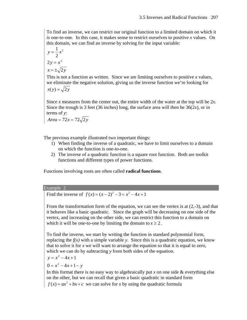
To find an inverse, we can restrict our original function to a limited domain on which it is one-to-one. In this case, it makes sense to restrict ourselves to positive x values. On this domain, we can find an inverse by solving for the input variable:

2

2

2

2

1

xy

xy

yx 2

This is not a function as written. Since we are limiting ourselves to positive x values, we eliminate the negative solution, giving us the inverse function we’re looking for

yyx 2)(

Since x measures from the center out, the entire width of the water at the top will be 2x. Since the trough is 3 feet (36 inches) long, the surface area will then be 36(2x), or in terms of y:

yxArea 27272

The previous example illustrated two important things:

1) When finding the inverse of a quadratic, we have to limit ourselves to a domain on which the function is one-to-one.

2) The inverse of a quadratic function is a square root function. Both are toolkit functions and different types of power functions.

Functions involving roots are often called radical functions. Example 2

Find the inverse of 143)2()( 22 xxxxf From the transformation form of the equation, we can see the vertex is at (2,-3), and that it behaves like a basic quadratic. Since the graph will be decreasing on one side of the vertex, and increasing on the other side, we can restrict this function to a domain on which it will be one-to-one by limiting the domain to 2x . To find the inverse, we start by writing the function in standard polynomial form, replacing the f(x) with a simple variable y. Since this is a quadratic equation, we know that to solve it for x we will want to arrange the equation so that it is equal to zero, which we can do by subtracting y from both sides of the equation.

yxx

xxy

140

142

2

In this format there is no easy way to algebraically put x on one side & everything else on the other, but we can recall that given a basic quadratic in standard form

2( )f x ax bx c we can solve for x by using the quadratic formula

Chapter 3

208

a

cabbx

2

))((4)()( 2 . We solve apply this to our equation 20 4 1x x y by

using 1a , 4b , and (1 )c y

2

4122

2

)1)(1(4)4()4( 2 yyx

Of course, as written this is not a function. Since we restricted our original function to a domain of 2x , the outputs of the inverse should be the same, telling us to utilize the + case:

2

4122)(1 y

yfx

Try it Now

1. Find the inverse of the function 2( ) 1f x x , on the domain 0x While it is not possible to find an inverse of most polynomial functions, some other basic polynomials are invertible. Example 3

Find the inverse of the function 15)( 3 xxf This is a transformation of the basic cubic toolkit function, and based on our knowledge of that function, we know it is one-to-one. Solving for the inverse by solving for x

31

3

3

3

5

1)(

5

1

51

15

yyfx

xy

xy

xy

Notice that this inverse is also a transformation of a power function with a fractional power, x1/3. Try it Now

2. Which toolkit functions have inverse functions without restricting their domain?


209

Besides being important as an inverse function, radical functions are common in important physical models. Example 4

The velocity, v in feet per second, of a car that slams on its brakes can be determined based on the length of skid marks that the tires leave on the ground. This relationship is given by

gfddv 2)(

In this formula, g represents acceleration due to gravity (32 ft/sec2), d is the length of the skid marks in feet, and f is a constant representing the friction of the surface. A car lost control on wet asphalt, with a friction coefficient of 0.5, leaving 200 foot skid marks. How fast was the car travelling when it lost control? Using the given values of f = 0.5 and d = 200, we can evaluate the given formula:

sec/80)200)(5.0)(32(2)200( ftv , which is about 54.5 miles per hour.

Radical functions raise important question of domain when composed with more complicated functions. Example 5

Find the domain of the function )1(

)3)(2()(

x

xxxf

Since a square root is only defined when the quantity under the radical is non-negative,

we need to determine where 0)1(

)3)(2(

x

xx. A rational function can change signs

(change from positive to negative or vice versa) at horizontal intercepts and at vertical asymptotes. For this equation, the graph could change signs at x = -2, 1, and 3. To determine on which intervals the rational expression is positive, we could evaluate the expression at test values, or sketch a graph. While both approaches work equally well, for this example we will use a graph. This function has two horizontal intercepts, both of which exhibit linear behavior, where the graph will pass through the intercept. There is one vertical asymptote, linear, leading to a behavior similar to the basic reciprocal toolkit function. There is a vertical intercept at (0, 6). This graph does not have a horizontal asymptote, since the degree of the numerator is larger than the degree of the denominator.

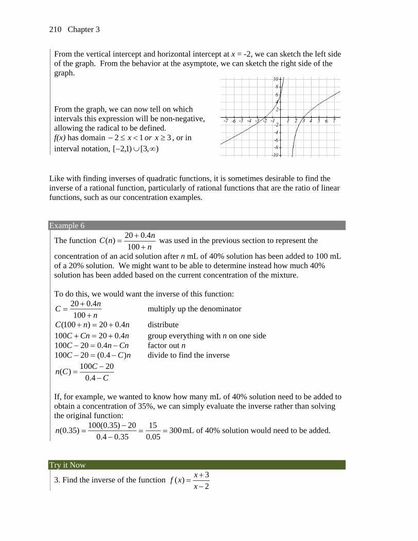
Chapter 3

210

From the vertical intercept and horizontal intercept at x = -2, we can sketch the left side of the graph. From the behavior at the asymptote, we can sketch the right side of the graph. From the graph, we can now tell on which intervals this expression will be non-negative, allowing the radical to be defined. f(x) has domain 312 xorx , or in interval notation, ),3[)1,2[

Like with finding inverses of quadratic functions, it is sometimes desirable to find the inverse of a rational function, particularly of rational functions that are the ratio of linear functions, such as our concentration examples. Example 6

The function n

nnC

100

4.020)( was used in the previous section to represent the

concentration of an acid solution after n mL of 40% solution has been added to 100 mL of a 20% solution. We might want to be able to determine instead how much 40% solution has been added based on the current concentration of the mixture. To do this, we would want the inverse of this function:

n

nC

100

4.020 multiply up the denominator

nnC 4.020)100( distribute nCnC 4.020100 group everything with n on one side

CnnC 4.020100 factor out n nCC )4.0(20100 divide to find the inverse

C

CCn

4.0

20100)(

If, for example, we wanted to know how many mL of 40% solution need to be added to obtain a concentration of 35%, we can simply evaluate the inverse rather than solving the original function:

30005.0

15

35.04.0

20)35.0(100)35.0(

n mL of 40% solution would need to be added.

Try it Now

3. Find the inverse of the function 3

( )2

xf x

x


211

Important Topics of this Section Imposing a coordinate system Finding an inverse function Restricting the domain Invertible toolkit functions Rational Functions Inverses of rational functions

Try it Now Answers

1. 1)(1 yyfx

2. identity, cubic, square root, cube root, exponential and logarithmic

3. 1 2 3( )

1

yf y

y

Chapter 3

212

Section 3.5 Exercises For each function, find a domain on which the function is one-to-one and non-decreasing, then find an inverse of the function on this domain.

1. 24f x x 2. 2

2f x x

3. 212f x x 4. 29f x x

5. 33 1f x x 6. 34 2f x x

Find the inverse of each function

7. 9 4 4f x x 8. 6 8 5f x x

9. 39 2f x x 10. 33f x x

11. 2

8f x

x

12. 3

4f x

x

13. 3

7

xf x

x

14. 2

7

xf x

x

15. 3 4

5 4

xf x

x

16. 5 1

2 5

xf x

x

Police use the formula 20v L to estimate the speed of a car, v, in miles per hour, based on the length, L, in feet, of its skid marks when suddenly braking on a dry, asphalt road. 17. At the scene of an accident, a police officer measures a car's skid marks to be 215 feet

long. Approximately how fast was the car traveling?

18. At the scene of an accident, a police officer measures a car's skid marks to be 135 feet long. Approximately how fast was the car traveling?

The formula 2.7v r models the maximum safe speed, v, in miles per hour, at which a car can travel on a curved road with radius of curvature r, in feet. 19. A highway crew measures the radius of curvature at an exit ramp on a highway as

430 feet. What is the maximum safe speed?

20. A highway crew measures the radius of curvature at a tight corner on a highway as 900 feet. What is the maximum safe speed?


213

21. A drainage canal has a cross-section in the shape of a parabola. Suppose that the canal is 10 feet deep and 20 feet wide at the top. If the water depth in the ditch is 5 feet, how wide is the surface of the water in the ditch? [UW]

22. Brooke is located 5 miles out from the nearest point A along a straight shoreline in her seakayak. Hunger strikes and she wants to make it to Kono’s for lunch; see picture. Brooke can paddle 2 mph and walk 4 mph. [UW]

a. If she paddles along a straight line course to the shore, find an expression that computes the total time to reach lunch in terms of the location where Brooke beaches the boat.

b. Determine the total time to reach Kono’s if she paddles directly to the point A. c. Determine the total time to reach Kono’s if she paddles directly to Kono’s. d. Do you think your answer to b or c is the minimum time required for Brooke

to reach lunch? e. Determine the total time to reach Kono’s if she paddles directly to a point on

the shore half way between point A and Kono’s. How does this time compare to the times in parts b or c? Do you need to modify your answer to part d?

23. Clovis is standing at the edge of a cliff, which slopes 4 feet downward from him for every 1 horizontal foot. He launches a small model rocket from where he is standing. With the origin of the coordinate system located where he is standing, and the x-axis extending horizontally, the path of the rocket is described by the formula

22 120y x x . [UW]

a. Give a function ( )h f x relating the height h of the rocket above the sloping

ground to its x-coordinate. b. Find the maximum height of the rocket above the sloping ground. What is its

x-coordinate when it is at its maximum height? c. Clovis measures its height h of the rocket above the sloping ground while it is

going up. Give a function x g h relating the x-coordinate of the rocket to

h. d. Does this function still work when the rocket is going down? Explain.

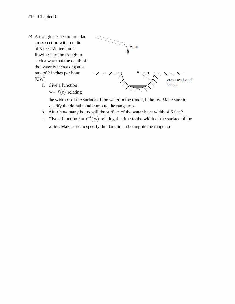
Chapter 3

214

24. A trough has a semicircular

cross section with a radius of 5 feet. Water starts flowing into the trough in such a way that the depth of the water is increasing at a rate of 2 inches per hour. [UW]

a. Give a function

w f t relating

the width w of the surface of the water to the time t, in hours. Make sure to specify the domain and compute the range too.

b. After how many hours will the surface of the water have width of 6 feet?

c. Give a function 1t f w relating the time to the width of the surface of the

water. Make sure to specify the domain and compute the range too.

chapter 3: polynomial and rational functions 3.pdf · section 3.3 graphs of polynomial functions...

Documents