chapter 3 the alpha-magnet · chapter 3 the alpha-magnet as will be discussed fully in chapter 4,...
TRANSCRIPT
Chapter 3
The Alpha-Magnet
As will be discussed fully in Chapter 4, the beam directly out. of the gun is not, suitable
for injection into a S-band linear accelerator section. Doing so would produce an
accelerated beam with a large energy spread because of the large phase-spread the
particles coming into the accelerator section would have in the absence of compression.
Magnetic bunch compression is one solution to this problem, and the one which is
most’ suitsable for use with the RF gun. Indeed, the possibilit’y of using magnetic
compression, as opposed to RF bunching, is one of t,he at.tractive feat,ures of the RF
gun.
The t*heory of magnetic compression will be discussed fully in the next chapt,er,
along with t,he motivation for using an alpha-magnet. In this chapt.er, I will describe
t.he alpha-magnet’ and derive its main properties. First,, I will discuss t.he magnet’ic
design of t.he SSRL alpha-magnet: which is an asymmetric quadrupole, and contrast
this design with an alt,ernative design, namely a Panofsky quadrupole. Second, I will
present, t.he equation of motion in an alpha magnet., and show how a scaled form of the
differential equation can be used t,o deduce some of the magnet’s properties, without,
int$egrat,ion. I will prove that, the transport matrices for any alpha magnet. can be
expressed in terms of transport. mabrices for this scaled equation of motion. I will show
how these lat,ter transport, matrices can be derived from fit,s to the results of numerical
integration of the scaled equation of motion for an appropriately selectsed ensemble
of particles. I will present, the results of a calculation of alpha-magnet, transport,
ma.trices to t.hird order, along with discussion of the accuracy of the results. Having 132

CHAPTER3. THEALPHA-MAGh7ET 133
calculat.ed matrices for a perfect alpha-magnet, I then discuss how to extend the
treatment. t.o imperfect, alpha-magnets, specifically those with multipole and beam-
hole-induced field errors. Finally, I present, the results of experimental measuremenbs
of the SSRL alpha-magnet, including magnetic measurements and measuremenbs of
some first.-order matrix elements.
--

CHAPTER3. THEALPHA-MAGNET 134
3.1 Magnetic Characteristics and Design of the
Alpha-Magnet
The alpha-magnet. and its properties were first, described by Enge[45]. It’ is essentially
half of a quadrupole magnet, with a symmet,ry plane at qi = 0, i.e., with a vertical
mirror plane along the longitudinal axis. This mirror plane provides the symmet,ry
necessary to obt,ain quadrupole-like fields in the interior of t’he magnet. Figure 3.1,
a simplified cross-sect,ional view of the alpha-magnet, designed for t,he SSRL project,
illust,rabes these point’s and ant,icipat,es the discussion to follow. Rather than inject’
t,he beam along t#he quadrupole axis (as might, be done if the magnet, where to be
used as a combined-function dipole and quadrupole), t.he beam is injecbed through
t’he “front,-plat,e”, i.e.. through the iron piece that. functions as an approximation t,o
an ideal magnet’ic mirror-plane.
3.1.1 Asymmetric Quadrupole Design
To understand t.his in more detail, it is convenient, t,o use t.he approximation that
t,he permeabilit~y of iron is infinite. In this case, Maxwell’s equat,ions at a mat.erial
boundary mandate t,hat t.he magnetic field H just, out.side t,he iron be perpendicular
to t.he iron surface. (For a full discussion of several of the points that’ follow, see
J.D.Jackson, [31].) I6 follows t.hat t,he iron surfaces are equipodentials of t.he magnet’ic
scalar pot,ent*ial @ M, which is related to t’he magnet’ic field by
B=H=-V9eM, (3.1)
where I employ Ga.ussian unit,s, and use the fact, t.hat’ B = H in air.
An infinitely-long quadrupole magnet. is defined as one t,hat’ has a magnetic field
given by
B = g(qA + q&L (3.2)
where g is t.he quadrupole gradient, and where qi, 42, and& form a right-handed coor-
dinat,e system (The reason for t*he unusual choice of coordinat.es-( qi , 92, qa) inst.ead
of the usual (x, y, z)-is for consist,ency wit,h subsequent, sectsions of this chapt,er.) The

.
CHAPTER 3. THE ALPHA-MAGNET
I I
1 I I I I I 1
135
Figure 3.1: Simplified Cross-sectional view of the SSRL alpha-magnet.
--

.
CHAPTERS. THEALPHA-MAGNET 136
reader can verify that. this field satisfies Maxwell’s equations, and also t,hat it, can be
derived from t.he magnetic pot.ential
@Q = -gql%- (34
Knowing the magnetic pot,ential necessary to produce quadrupolar magnetic fields
allows one to specify t,he location of equipotential surfaces that will produce such a
field. That is, if one arranges magnetic surfaces and suitable driving currents so as to
obtain equipotent,ials of a quadrupolar field on the magnetic surfaces, then the region
inside the boundary formed by the magnetic surfaces will conk& a quadrupolar field
dist,ribution. While it. is by no means essent,ial to do so, this is t,ypically accomplished
by a four-fold symmedric arrangement of iron, where alternate poles of t,he magnet’
have the same pot,ential except for a change in sign. Since the magnet poles are
equipotentials, they must be hyperbolic in shape. (This brief exposition does not.
show the full- power of the equipot,ential method in treating multi-pole fields, for
which the reader should consult, ot,her sources.[6])
From the definibion of the quadrupole field, it. follows that the lines ql = 0 and
qa = 0 are equipotentials with @ = 0. Hence, if a magnetic surface is placed along the
line qi = 0 ext,ending into qi < 0, then the field in the region qi > 0 is unchanged,
since the locations and shapes of t.he equipot,ent,ials are unchanged. This is what’ is
done for- the asymmetric quadrupole alpha-magnet, design used for the SSRL project,.
The reader is referred again to Figure 3.1, which exhibits the truncat,ed hyperbolic
poles and the mirror-p1at.e along qi = 0. This design is called “asymmet,ric” because
the hyperbola extends further horizontally than vertically, in order to obtain a large
horizontal good field region. The deviation from the hyperbolic equipotential surface
that is implied by truncateion of the hyperbola is made up for by “shiming” the pole
with additional magnetic mat.erial near the upper end of t’he hyperbola. This is a
trail-and-error process that. was carried out using t.he magnet, code POISSON[66].
The resultant calculat.ed gradient in the qa = 0 plane is shown in Figure 3.2, along
wit,h measurements performed on the magnet before the beam ent,rance/exit’ hole was
cut, in the mirror plat,e. Not,e that the way the data is normalized means t,hat. one
should compare t.he shapes of t#he curves rather t,han the absolut,e agreement. I used
a linearized Hall probe for t,hese measurements (as well as those present,ed below),

.
CHAPTER3. THEALPHA-MAGNET 13i
Figure 3.2: Computed and Measured Gradient of the SSRL Alpha-Magnet,
--

CK4PTER3. THEALPHA-MAGNET
vB (G/cm)
Figure 3.3: Measured Excitation Curve of the SSRL Alpha-Magnet,
138

CHd4PTER 3. THE ALPHA-MAGNET 139
t,o ensure t,hat spurious non-linearities did not. appear in the dat,a. The discrepancies
are believed to be due in part to construction errors in the magnet., which resulted in
deviations of the pole profile from the design. Some of the discrepancies are also due
t,o round-off errors and convergence problems in POISSON, which cause the gradient’
near ql = 0 t.o become non-uniform. In any case, the non-uniformities of the gradient,
for the magnet without a beam port. are dwarfed by t.hose introduced when the beam
port, is cut’ into the front’ plate. I will ret.urn to t.his t,opic later in this chapter. Figure
3.3 shows the measured excit.at,ion curve, along with a line showing extrapolating
the low-current’ region of t,he curve bo high currents, which illust,rat,es the effect, of
sat,urabion. Select.ed magnet, paramet’ers are listed in Table 3.1.
Table 3.1: SSRL Alpha-Magnet Design Parameters.
number of t,urns maximum current maximum gradient.
inscribed pole radius good-field region (extent, in ql) gradient unif0rmit.y wit,hout, beam port’ depth (ext*ent’ in 92) resistance ner coil Q 45°C
80 260 A
405 G/cm 10 cm 20 cm
.5% 40 cm 40 mS2
3.1.2 Panofsky Quadrupole Design
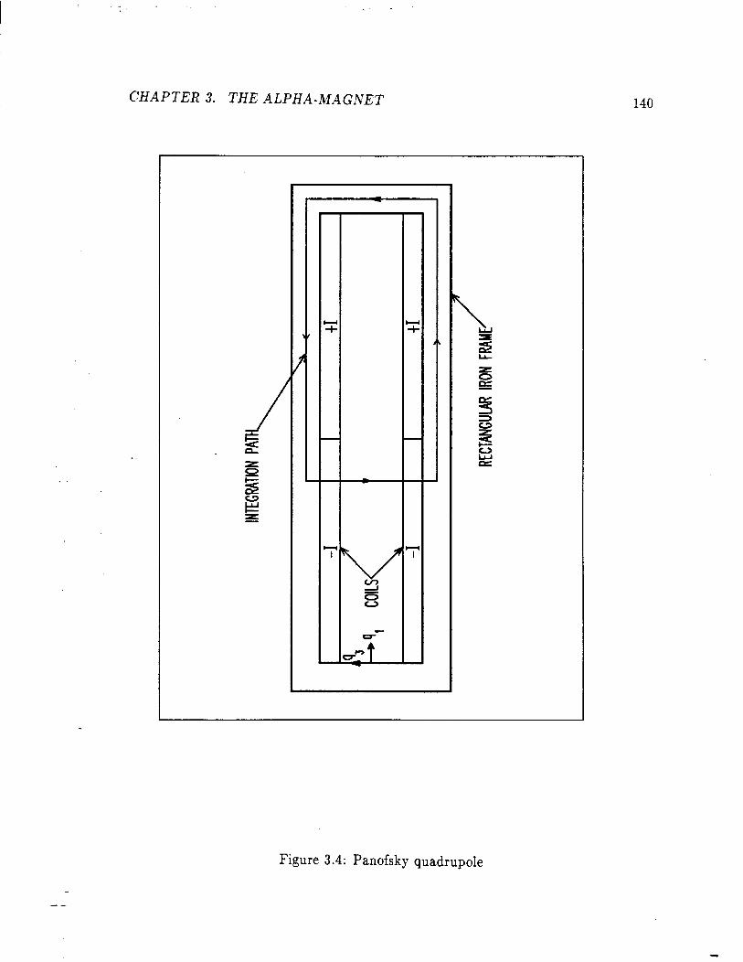
Another magnet design that, might. be employed inst,ead of t.he asymmet.ric quadrupole
used here is a half Panofsky quadrupole [67] depicted in Figure 3.4. Unlike standard
quadrupole designs where the quadrupole field is obtained through the approximat,ely
hyperbolic shape of t’he poles, the Panofsky quadrupole relies on uniform sheets of
current to produce a quadrupole field. From 3.4 it. can be seen that. J f 0 at the pole
surfaces, from which it, follows that’ the fields in the magnet gap are not det.ermined
solely by t,he shape of the poles, in contrast’ to t.he sit,uat,ion for a standard qua.d-
rupole design. The most, st,raight-forward way to calculate the fields in a Panofsky
.
CHAPTER 3. THEALPHA-MAGNET 140
Figure 3.4: Panofsky quadrupole
--

.
CHAPTER 3. THE ALPHA-MAGNET
quadrupole is t,o use the integral form of Ampere’s law:
J H . dl = 5. C
141
(3.4)
In more practical units, this can be written as[S]:
J H - dl = 0.4~1, (3.5)
where H is in Gauss, 1 is in cm, and I is in Ampere-turns. Taking t.he int,egration
loop as shown in 3.4 and assuming infinit,e permeabilit.y and t.hat’ H, is a function of
x only (which must, be approximat,ely true for a magnet, that’ is wide compared 60 its
gap- height.), one obtains
H3 = 0.8?iF, (3.6)
where h is the full gap of the magnet, J is the current, density in the current, sheets,
and t. is the t,hickness of the current, sheets. _. The linear dependence of Ha on ql
demonstrat,es that. this is indeed a quadrupole. In order to obtain Hl, one employs
V x H = 0, from which it’ follows that.
(3.7)
By comparison with equation (3.2), it. is seen that, the magnet in Figure 3.4 is, in fact.,
a quadrupole, with gradient, 0.4T
g= hJt,, (3.8)
where J is in A/cm*, g is in G/cm and t, and h are in cm.
3.1.3 Comparison of the Two Designs
A major difference between the Panofsky and asymmetric quadrupole designs for the
alpha magnet. is the amount. of power consumed t,o produce a given gradient in a
specified region. It, is this difference that, lead to the adoption of t,he asymmet,ric
design for the SSRL project.
To investigate t,his, I will assume that’ what. is desired is an alpha magnet’ wit,h
depth D (as perceived in Figures 3.1 and 3.4), useful gap h,, and good field region G,
CHAPTERS. THEALPHA-MAGNET 142
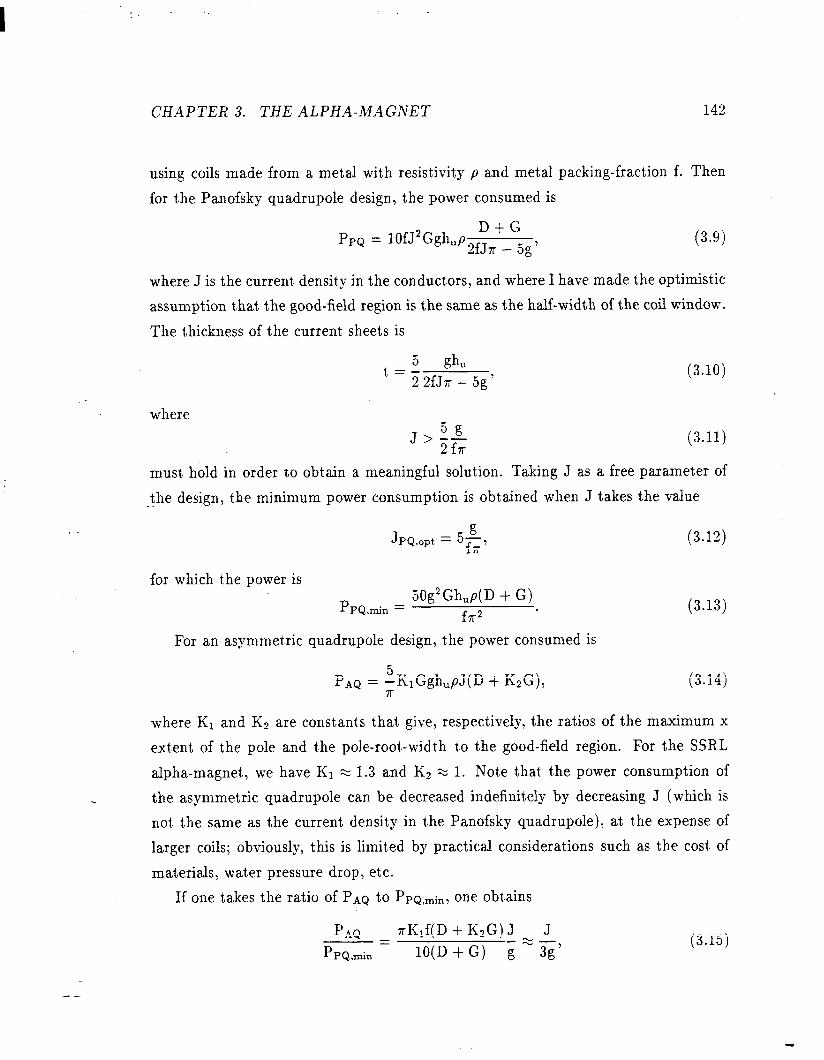
using coils made from a metal with resist,ivity p and metal packing-fraction f. Then
for t,he Panofsky quadrupole design, the power consumed is
PpQ = lOfJ*Ggh,p D + G 2fJr - 5g’
(3.9)
where J is the current. densit,y in the conductors, and where I have made the optimistic
assumption t,hat. the good-field region is the same as the half-width of the coil window.
The thickness of t.he current, sheets is
(3.10)
where
(3.11)
must, hold in order to obtain a meaningful solution. Taking J as a free parameber of
t,he design, t,he minimum power consumption is obtained when J takes the value _.
g JPQ,~~~ = 5-,
f7r (3.12)
for which the power is
PPQ,min = 50g*Gh,p(D + G)
f.rr2
For an asymmet.ric quadrupole design, the power consumed is
PAQ = zKiGgh,pJ(D + KzG),
(3.13)
(3.14)
where Kl and K2 are constanbs that, give, respectively, the ratios of the maximum x
extent of t.he pole and the pole-root,-widt,h to the good-field region. For the SSRL
alpha-magnet, we have Ki z 1.3 and K2 z 1. Notme that, the power consumption of
the asymmetric quadrupole can be decreased indefinitely by decreasing J (which is
not, the same as the current densit.y in the Panofsky quadrupole), at, the expense of
larger coils; obviously, this is limit,ed by practical considerations such as the cost, of
materials, water pressure drop, etc.
If one takes the ratio of PAQ to PpQ,min, one obtains
pAQ = rKif(D + K2G)J - J
P PQ,min lO(D + G) g - c’ (3.15)

.
CHAPTERS. THEALPHA-MAGNET 143
where I ignore fact,ors of order unity in making t,he approximation. The maximum
gradient’ desired in the SSRL applicat,ion was 350 G/cm2. Hence, the Panofsky quad-
rupole would have used more power unless the current densit$y for the asymmet.ric
quadrupole were above about 1000 A/cm2. In fact, the coils in t,he magnet, could be
made large enough to achieve J 5 175A/cm2, from which one can conclude that. a
comparable Panofsky quadrupole would consume about’ six times as much power as
the design used.

CHAPTER3. THEALPHA-MAGNET 144
3.2 Particle Motion in the Alpha-Magnet
3.2.1 Scaled Equation of Motion
Particle motion in the alpha-magnet, is best. described with the aid of a diagram such
as Figure 3.5, which shows the cent.raI particle trajectory and the coordinate syst,em.
In t,erms of t,hese coordinates, the magnetic field for q1 > 0 is
B = gkm + wd, (3.16)
where t,he constant, g is bhe alpha-magnet, gradient. The equat.ion of motion is obtained
from t,he Lorent,z force
F=-eE+?vxB, C
(3.17)
with E = 0, and is
_.
drv e v x B -=-- dt m,c *
(3.18)
Since t,he magnetic field does no work, y is constant, and can be taken outside t,he
derivabive. Since the magnitude of t.he velocit,y is also constant, one can rewrit,e
t.he derivatives as derivat,ives wit.h respect, to path-lengt,h, s = pet,, instead of t,ime.
Combining these, one obtains
d2q e %B
- = -m,c2p7 ds ds2 ’ (3.19)
I now define a constant, 0 by
a2 = eg
mec2i% ’ (3.20)
or, in more pract,ical units
a2 = 5.86674 x 10⁻⁴cm- 2 gwc4
P-Y *
The equat.ion of motion becomes
d2s 2dq B(q) - = -a-x- ds2 ds .!z
= --Q 2 q
$x(93mk)
dq3 dql dq2 = --Q -g3 - -j-p? -p3
(3.21)
(3.22)
(3.23)
(3.24)

-
CHAPTER 3. THEALPHz4-M.4GNET
Figure 3.5: Alpha-magnet co0rdinat.e system
--
.
CHAPTER 3. THE ALPHA4-MAGNET 146
I chose by convent,ion t.o make g > 0, i.e., I define t.he es axis to obt,ain B3 > 0
inside t,he magnet,. This also ensures that, a2 > 0, so that. a is real and positive. To
obtain an a-like t.raject#ory like that. exhibitsed in Figure 3.5, it is then necessary to
have initial velocities such that
dql ds’O and $0
ds * (3.25)
I wish to rewribe this equat,ion of motion once more, in such a way as t,o scale out.
all explicit dependence on g and Pr. To do this, I define scaled coordinat,es Q = qQ
and scaled pat,h-length S = sa. Using t’his, I obtain
d2Q dQ Qa - = -dS xB(-)- dS2 Q g
dQ = -dS x (Q3A Qd
dQz = - -QI? SQs - $41, -zQz) dS
Not.e that’
(3.26)
(3.27)
(3.28)
(3.29)
a result, which will be useful latter, and which in fact, does not depend on the scaling
(it is true of 2 as well).
3.2.2 Ideal Trajectory
From this result, one can deduce that, an alpha-magnet can act, like an achromat.ic
magnetic mirror, that is, that. a zero-emit,tance beam injected at a specific angle, 19,,
to the normal into a perfect. alpha-magnet will emerge at the point, of injection, at.
t*he same angle to the normal and undispersed in moment.um.
To see t,his, first. note t.hat. the scaled form of the equat.ion of motion does not,
display any dependence on moment,um. Hence, t,he Qrajectories of particles wit,h
various momenta injected int.o t,he magnet. at, the same angle are simply magnifications
or demagnifications of one another. Since t,he scaled equation likewise does not exhibit,
any dependence on gradient,, the same can be said of particles inject,ed int,o alpha
magnets witch differing gradient.s. Because the scaling involves all coordinates, it,
CHAPTER 3. THE ALPHA-MAGNET 147
leaves angles unchanged. Hence, if a closed, a-like trajecdory does exist, it has the
same shape and the same incident. and final angles for all values of a (i.e., for particles
of all momenta in alpha magnets of all gradients).
Not#e that, the scaling alone is not sufficient, t.o ensure that the magnet, can be
operated as an achromat. It is also necessary that. a traject.ory exists which exits at’
the injection point,, since ot.herwise the scaling would change the exit, locat,ion relative
to the injection point. This would, of course, imply non-zero dispersion upon exiting
t,he magnet.
-
Next, set. Qs = 0 and not,e that, for traject,ories st,art,ed at’ Q2 = 0 widh 2 = 0
(implying $$ = 1) there is some initial value, Q1, of Q1 t,hat results in a traject,ory
t.hat crosses Q1 = Q2 = 0. To see that. this must. be so, imagine starting t,rajectories
from Q2 = 0 at various initial values of Q1. A traject,ory started at infinit,esimally
small Qi > 0 will cross Qr = 0 at’ infinit,y, since it “sees” very little magnetic field,
and hence is bent. toward Q1 = 0 only very gradually. As the starting Qi is increased, _. t.he trajectory crosses Qi = 0 at, less and less positive values of Q2, until eventually,
for initial Qi = ($1, the traject,ory crosses Qi = 0 at Q2 = 0.
I will denote this traject.ory by Q(S) = (~,(S),~,(S), 0), and let. S = 0 at t.he start.
of t,he traject,ory, which is formally defined only for S > 0. By const,ruction, Q(S) is
a solut,ion to the equations of motion. Consider a new traject,ory Q(S) defined for
S < 0 as (8,(-S), -Q2(-S), 0). Upon inserting this traject,ory into the equation of
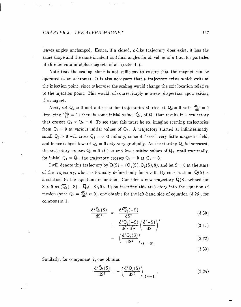
mot,ion (with Qs = s = 0): one obtains for t,he left,-hand side of equation (3.26), for
component 1:
d*&(S) d28,(-S) dS2 = dS2
= (S-+-S)
(3.30)
(3.31)
(3.32)
(3.33)
Similarly, for component’ 2, one obt,ains
d2&(S) = dS2
(3.34)
--
CHAPTER 3. THE ALPHA-MAGNET 148
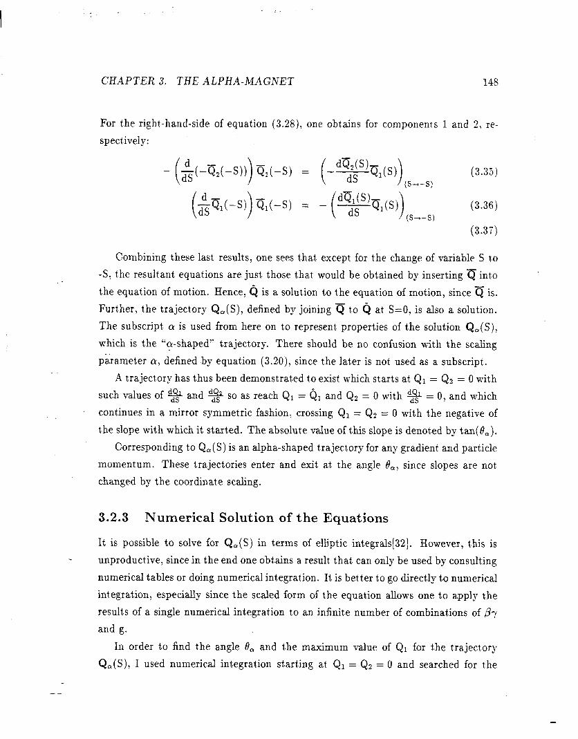
For the right-hand-side of equation (3.28), one obtains for component,s 1 and 2, re-
spect,ively:
- i
-&t-Q,(S))) w-s> = (- d~p21@~)
(&w) 8,(-S> = - ( dQpQds):
(3.35) (S--S)
I (3.36) (L-S)
(3.37)
Combining these last, results, one sees that, except for t.he change of variable S to
-S: t.he result’ant, equations are just, those t,ha,t. would be obtained by inserting Q int,o
the equation of mot,ion. Hence, Q is a solution t,o the equat,ion of motion, since Q is.
Furt.her, the trajectory QQ(S), defined by joining Q to 0 at S=O, is also a solut.ion.
The subscript, Q is used from here on to represent, properties of the solution Qa(S),
which is t,he “a-shaped” kajectory. There should be no confusion with the scaling
parameter Q, defined .by equat,ion (3.20), since the lat,er is not. used as a subscript.
A traject,ory has thus been demonstrat.ed to exist which starts at Q1 = Q2 = 0 with
such values of 9 and 9 so as reach Q1 = Qi and Q2 = 0 wit,h $$ = 0, and which
cont,inues in a mirror symmetric fashion, crossing Qi = Q2 = 0 with t,he negat,ive of
t,he slope with which it, start,ed. The absolut,e value of this slope is denot*ed by tan(8,).
Corresponding to QQ( S) is an alpha-shaped trajectory for any gradient, and particle
momentum. These trajectories enter and exit, at’ the angle t?,, since slopes are not,
changed by the co0rdinat.e scaling.
3.2.3 Numerical Solution of the Equations
It’ is possible to solve for Qa(S) in terms of ellipt.ic integrals[32]. However, this is
unproduct,ive, since in the end one obtains a result. that can only be used by consulting
numerical tables or doing numerical integration. It, is bedter to go directly to numerical
int,egrat,ion, especially since the scaled form of t,he equation allows one t,o apply the
results of a single numerical integrat,ion to an infinite number of combinations of Pr
and g.
In order t,o find t,he angle 8, and the maximum value of Qi for the tra.jectory
Qa(S), I used numerical integration start.ing at, Qi = Q2 = 0 and searched for the
CHAPTERS. THEALPHA-MAGNET 149
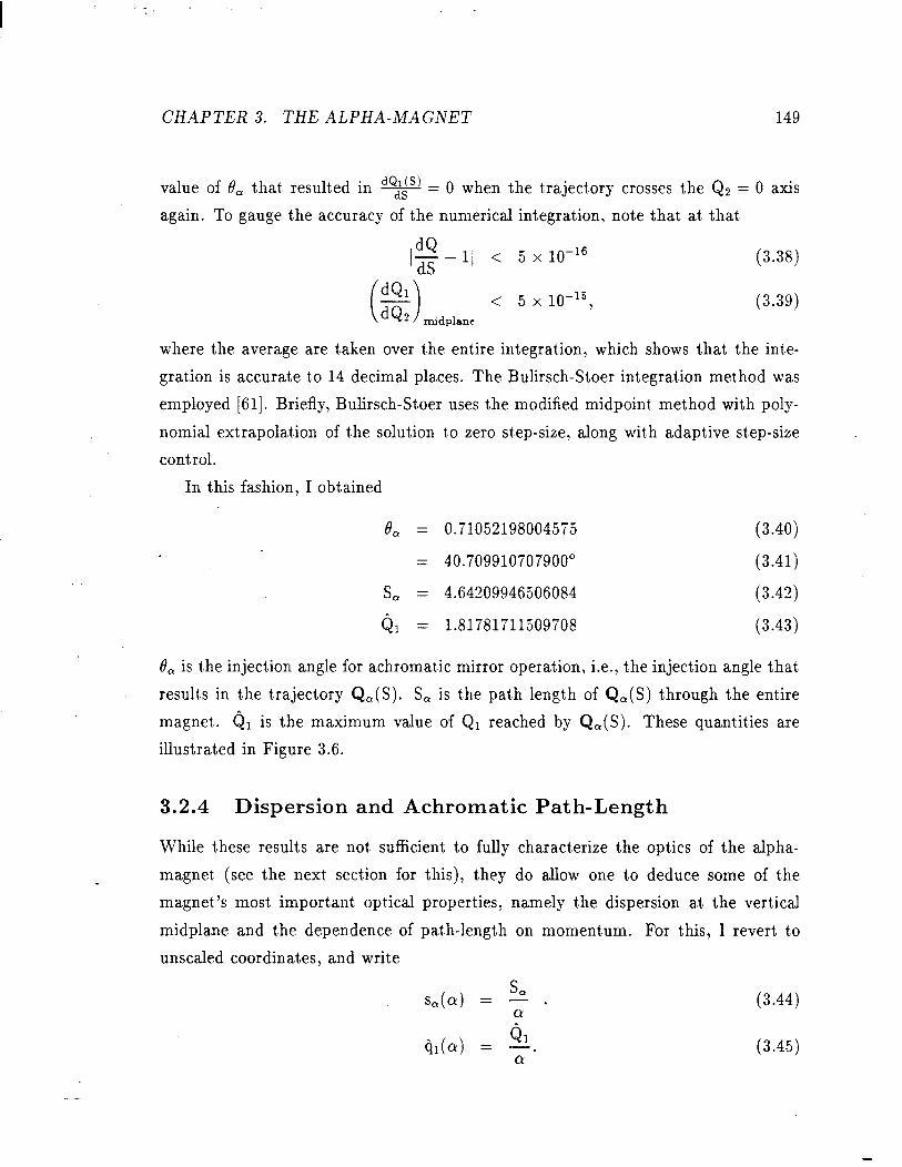
value of 8, t.hat, resultfed in v = 0 wh en the t#raject.ory crosses the Q2 = 0 axis
again. To gauge t,he accuracy of the numerical integration, not.e that ab that
l/ < 5 x lo-i6
dQ1 c-1 d&2 < 5 x lo-r5,
midplane
(3.38)
(3.39)
where the average are t,aken over the entire integration, which shows that the inte-
gration is accurate t,o 14 decimal places. The Bulirsch-Stoer integrat,ion method was
employed [61]. Briefly, Bulirsch-Stoer uses the modified midpoint’ method with poly-
nomial extrapolation of the solution t.o zero step-size, along wit,h adaptive step-size
cont,rol.
In t.his fashion, I obt,ained
8, = 0.710521980045i5 (3.40) . .
= 40.709910707900” (3.41)
S, = 4.64209946506084 (3.42)
Qr = 1.81781711509708 (3.43)
6, is the injection angle for achromatic mirror operaCon, i.e., t.he injection angle t,hat.
results in the trajectory Q,(S). S, is the pat&h length of Qa(S) t,hrough the entire
magnet,. Qi is the maximum value of Qr reached by Qa(S). These quantities are
illustrated in Figure 3.6.
3.2.4 Dispersion and Achromatic Path-Length
While t,hese results are not, sufficient to fully charact,erize t-he optics of the alpha-
magnet. (see the next. sect,ion for this), they do allow one t.o deduce some of the
magnet,‘s most important. optical properties, namely Qhe dispersion at, the vertical
midplane and the dependence of path-length on moment,um. For this, I revert, to
unscaled coordinates, and write
S,(Q) = % . L
Q&k) = 5. a
(3.45)

-
CHAPTER 3. THE ALPHA-MAGNET
\ - . -
150
In .
d
Q .
7-l
Figure 3.6: Ideal Trajectory in the Alpha-Magnet.
--

r
CHAPTER3. THEALPHA-MAGNET 151
In more practical units, and using t,he numerical values of S, and ($1 given above
s,(cm) = 191.655 Pr J .dWm)
(3.46)
qi(cm) = 75.0513 d
” dw=-d
(3.47)
Assuming that’ the gradient, g is fixed, and let,ting o, be the value of cr for the central
particle, of momentum p0 = (PT)~, the previous equations imply that,
s(a) = s(&J~
Qlb) = tllh)~.
Expanding in 6 = (p - pO)/p, one obt,ains
(3.48)
(3.49)
(3.50)
(3.51)
Using this expansion the dispersive terms of 6he transport. matrix (see t,he next, sec-
tion) from the entrance of the magnet to the “vert.ical midplane” (where the ideal
trajectory crosses q2 = 0 with ql = qi) are seen to be
(3.52)
(3.53)
(3.54)
(3.55)
(3.56)
(3.57)
Similarly, the path-length berms for transport, t.hrough t,he entire magnet are
156 = $(a,) (3.58)
I :
CHAPTER 3. THE ALPHA-MAGNET
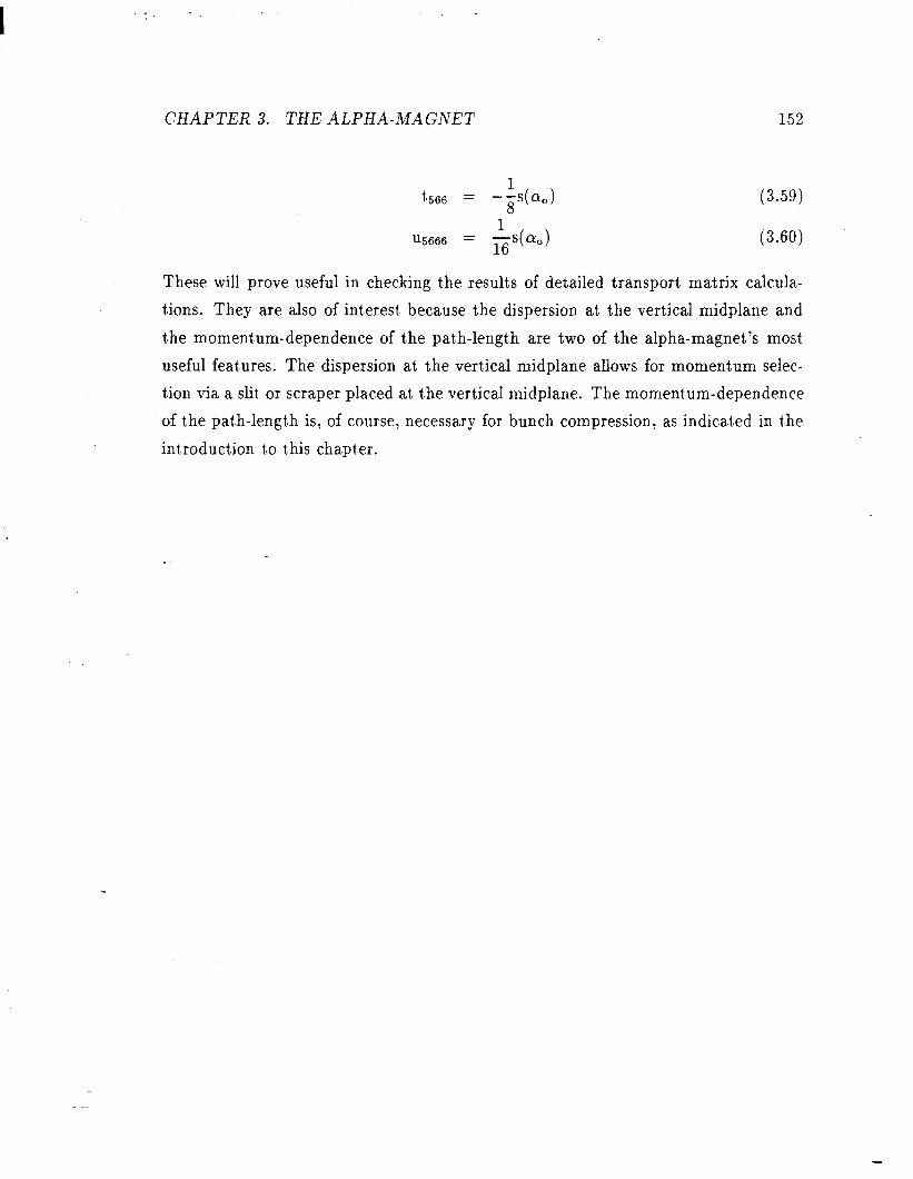
t566 = -&J
152
(3.59)
u5666 = (3.60)
These will prove useful in checking the results of det.ailed transport matrix calcula-
tions. They are also of interest, because t,he dispersion at, the vertical midplane and
the moment.um-dependence of the pat,h-length are two of the alpha.-magnet,‘s most’
useful feat.ures. The dispersion at the vert.ical midplane allows for momentum selec-
tion via a slit’ or scraper placed at, t,he vertical midplane. The moment,um-dependence
of the path-len@h is, of course, necessary for bunch compression, as indicat,ed in the
int.roduction t,o hhis chapt.er.

-
CHAPTER3. THEALPHA-MAGNET 153
3.3 Alpha-Magnet Transport Matrix Scaling
In this section I derive results that, provide the basis for a calculation of alpha-magnet.
transport, matrices t.o third order. Transport, matrices express particle mot.ion bet,ween
t#wo points in a beamline as a series expansion about the trajectory of a hypothetical
particle t,hat, travels along what, is considered t.o be the ideal trajectory for the beam-
line. Typically this ideal trajectory passes through the center of focusing elements,
down the center of the beam-pipe, and so forth. In t,he case of the alpha-magnet, t,he
ideal traject,ory enters and exits at, the angle 8,, wit.h q3 = % = 0.
3.3.1 Curvilinear Coordinates and Matrix Notation
The coordinat,es used for the transport, matrix expansion[lO] specify offsets in six-
dimensional phase-space of a particle from the ideal traject,ory. The coordinate syst’em
-is curvilinear; i.e., it’ follows the ideal kajectory. This subject is treat,ed completely in
publicat,ions on part,icle beam dynamics, Wed in t.he references. Here, I will simply
stat.e that. the position of any particle relative t.o the fiducial particle can be specified
in terms of t,wo transverse coordinat,es, x and y, their derivatives wit,h respect to path
lengt,h (s,) for t,he central t,rajecbory,
dx x’ = ds,
dy Y’= ds,’ (3.61)
the longit,udinal distance s kaveled, and the momentum deviat,ion 6, inkoduced
in t,he last. sect,ion. As is usually done, I form a six-dimensional vector from t,hese
coordinates: / \ x \
X’
Y x= Y’ *
S
\s/
(3.62)
This vector gives information about, a particle as it crosses a reference plane some-
where in t,he beamline. The reference plane is const,ructed so that, the fiducial particle
I :
CHAPTER3. THEALPHA-MAGNET 154
passes through it. perpendicularly. I emphasize that the path-length s is not t,he dis-
tance of a parMe behind the fiducial particle; I depart’ from convent.ion here in
keeping t,rack of the t,otal path-length, for reasons that, will be apparent, lat.er. This
carries no penalt.y for a beamline composed of st,atic elements, since t,he expansions
in s - so are then of no importance.
Transformation of this vect,or by beamline elements is expressed as a series expan-
sion:
Xi - Ci $ c rijxj $ c tijkxjxk + c uijklxjxkxl, (3.63) j jlk j/k>1
where c, r, t: and u are the transport, matrices for some element., and summation
indices run from 1 to 6 unless ot’herwise indicat,ed. (The reason for the lower-case
letters will be seen present,ly.) The restrict’ed sums are used t’o obt.ain expressions
that, comain only one instance of any t,erm xjxk or xjxkxl. This is consistent, with
K.Brown[lO], but. differs from the definit,ion used by TRANSPORT[68] and some
other computer programs, where the matrices are defined in terms of symmetric sums
over all indices. The unsymmetric form also has advant.ages in a compuber program,
namely reduction of st,orage used and reduct.ion of the number of arithmetic operations
needed t,o transform parbicle coordinat!es. I employ the unsymmetric form exclusively
in this work.
The element c is unconvent,ional, and is used to keep track of cent,roid offsets. It,
finds application in t.hree ways. First, when used in a tracking program, associat.ing a
cent’roid offset mat.rix with an element. allows one to implement, beam misalignments
and st,eering in a straight,-forward fashion. In addition, t.ime-of-flight, calculations are
facilitated by the pat,h-length centroid element, which is useful in a simulat,ion that,
has t.ime-dependent, elements [49]. Second, it is a necessary corrolary of my use of total
path-lengt,h instead of differential path-length in the vector x. Third, in the part,icular
case of the alpha-magnet, t,he centroid matrix can be used to calculate higher-order
dispersive path-lengt,h terms, as will be seen below. For the alpha-magnet, and all
ot.her element#s that, do not produce orbit. dist,ortions, only t,he cs element, is non-zero.

CHAPTER 3. THE ALPHA-h!AGNET 155
3.3.2 Relationships Between Curvilinear and Fixed Coor-
dinates
At. t,his point, the reader might. expect. the equat,ion of motion to be rewrit.ten in terms
of the curvilinear coordinat,es. This is unnecessary for my purposes. All that I will
need in order calculate t,he matrices (c, r, t,, u) is t,o express the relationship bet,ween
the curvilinear coordinat,es x and the coordinat.es of the equation of motion, q, at. the
entrance, vertical midplane, and exit, of the alpha-magnet, since it is bebween these
reference planes that. I wish t’o know the transport, matrices.
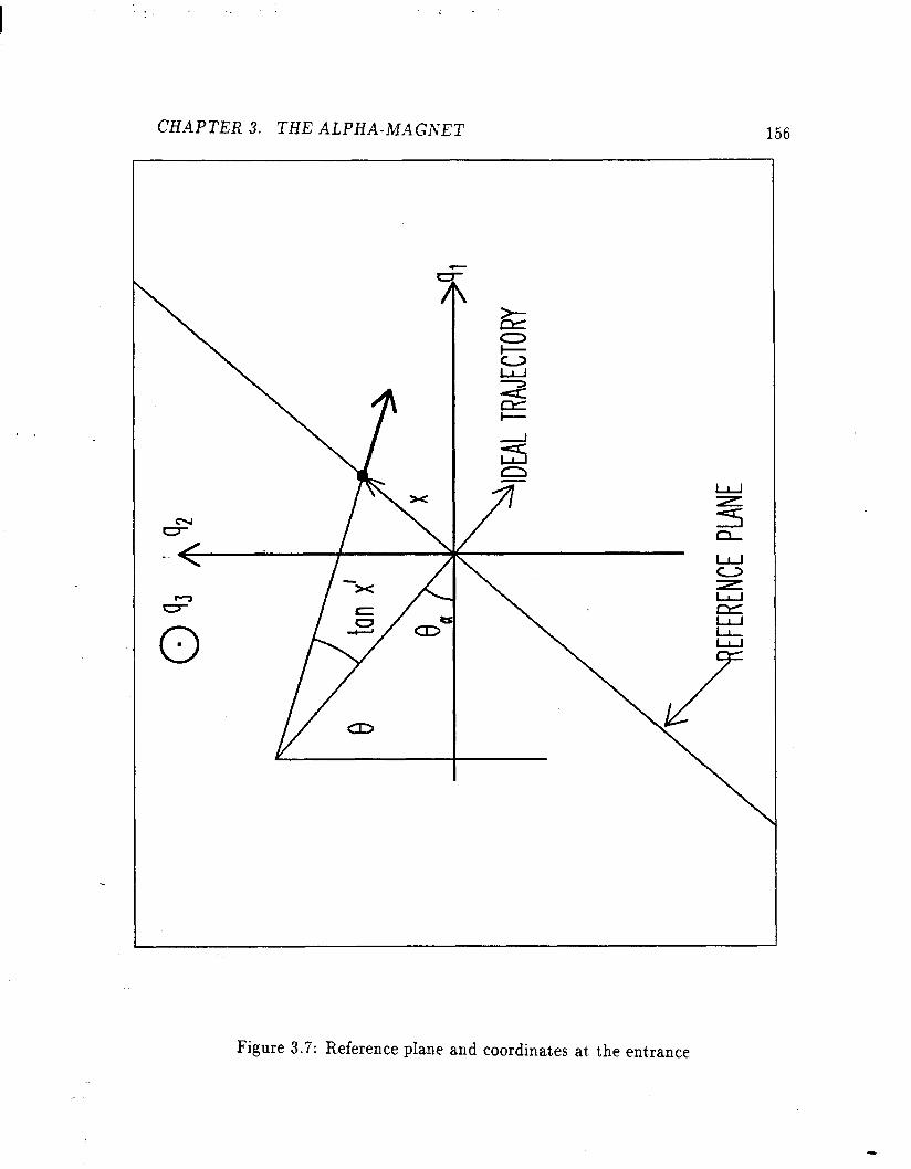
- At, the ent,rance of t,he alpha-magnet, (i.e., when t,he particle crosses the reference
plane shown in Figure 3.i), the correspondence bet.ween x and q is given by
X
X’
Y
Y’
I-
s
=
signh )j/ZG ’ tan(atan( -qi /qi) - 8,)
q3
sQ
S
(P - PO)/PO
where I have used
The slopes qi and qb are given by
qi = d-sin (8, + atan(
and
qi = Jmcos (8, + at,an(x’)),
while the coordinates q1 and q2 are given by
q1 = xsin8,
and
q2 = x cos 8,.
(3.64)
(3.65)
(3.66)
(3.67)
(3.68)
(3.69)
The reader may have not.iced that. the reference plane in Figure 3.7 is pardially
inside and parbially outside the alpha-magnet. Hence, it. would seem that in reaching
--
CH.4PT.M 3. THE ALPHA-MAGIVET 156
Figure 3.7: Reference plane and coordinates at, the entrance
-
CHAPTER 3. THE ALPHA-MAGNET 157
t.he reference plane, from which transport. through t.he alpha-magnet nominally starts
in the transport, matrix formalism, some particles have already traversed part’ of t,he
alpha-magnet.‘s magnet,ic field. Others (those for which x < 0 in figure 3.7), will
not. yet be inside the alpha-magnet. It. would seem that the lengt,h of a drift, space,
for example, prior to the alpha magnet’ would need to be modified according to the
coordinates of t.he particle, and this is effectively what is done. The prior element.
in the t.ransport line (presumably a drift’ space) is considered to deliver all of the
particles t,o the reference plane, with no account, taken of the alpha-magnet, fields.
The compubation of the alpha-magnet matrices (see the subsequent, sect,ions of this
chapt,er) takes bhis into account, so that, particles that are delivered inside (outside)
tShe alpha-magnet are drift.ed backward (forward) to the field boundary of the alpha-
magnet, before numerical integration. As will be seen presently, similar considerations
apply at the exit of the alpha-magnet, and an identical procedure is followed for this
cage.
One could also consider const,ructing an edge-matrix for the alpha-magnet, similar
t,o what, is done for bending magnets, but, since the entrance and exit, angles for the
alpha-magnet do not vary bet.ween applications (as t,hey do for bending magnets),
this is neit,her necessary nor useful.
At the vertical midplane of the magnet (i.e., when the particle crosses q2 = 0
inside the magnet, see Figure 3.8), a different relationship holds:
\
X
X’
Y
Y’
7
b,
=
a1 - 91
-cl:/4
q3
4
S
(P - PA/P
The slopes qi and qb are given by
I
qi = -41 - (q$)2 sin (atan(
and
qb = dwcos (atan(x
(3.70)
(3X)
(3.72)

.
CHAPTER3. THEALPHA-MAGNET 158
Figure 3.8: R.eference plane and coordinates at, bhe vertical midplane
--

CHAPTER3. THEALPHA-MAGNET
while the coordinates q1 and q2 are given by
159
41 = 41 -x (3.73)
and
q2 = 0. (3.74)
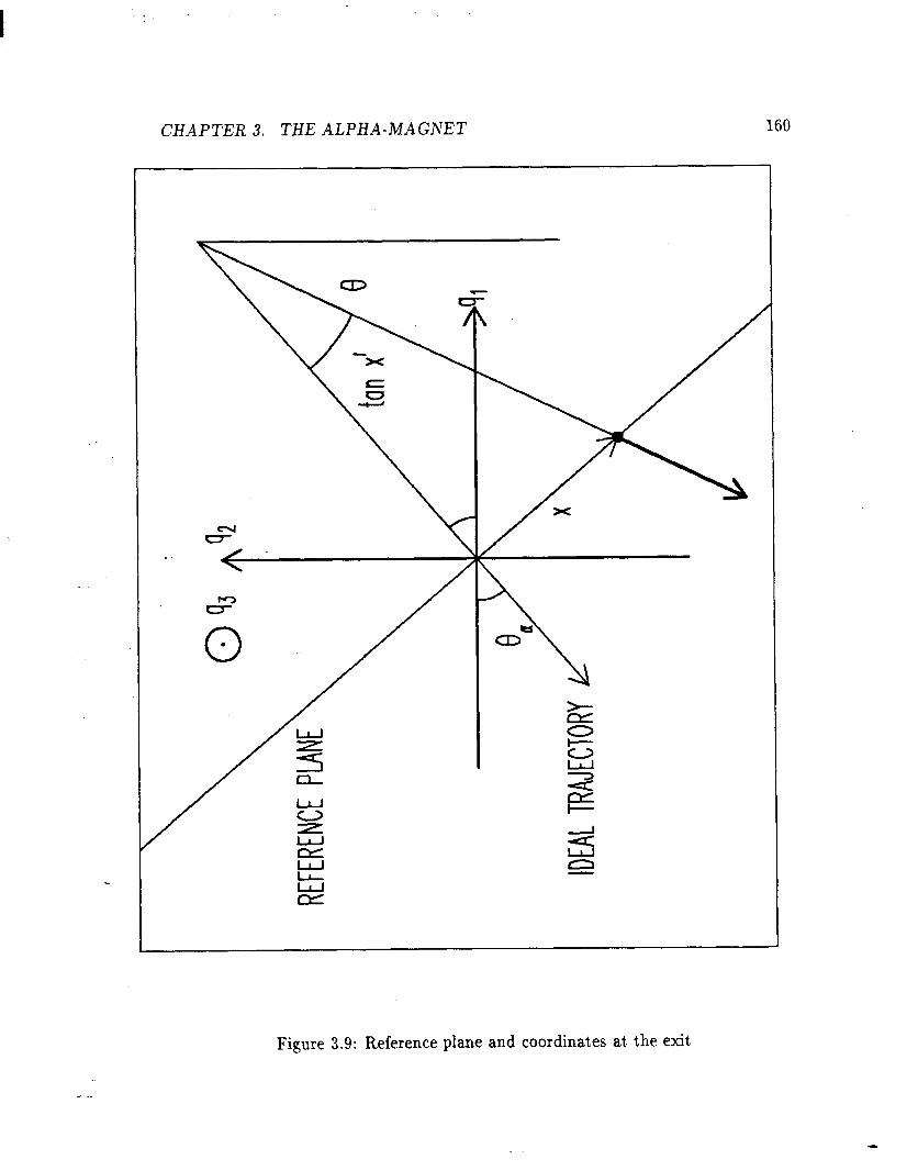
Finally, at. the exit, of the magnet, (i.e., when the particle crosses the reference
plane shown in Figure 3.9), one obtains:
X
X’
Y
Yt 7
6
=
The slopes qi and q$ are given by
QPhl > ~sx
t.an( S, - atan( qi /qi))
q3
Q$
S
(P - PO)/P
(3.75)
and
s’l = -t/l - b&l2 sin (f?, - atan( (3.76)
q; = -Jecos (@, - at.an(x’)),
while the coordinates ql and q2 are given by
qr = xsin8,
and
q2 = -xcose,.
(3.77)
(3.T8)
(3.79)
3.3.3 Coordinate Scaling
Let the gradient, in the alpha-magnet and the momentum of t,he fiducial particle be
specified, so that the scaling parameter Q takes a definite value, oO. Then it, is possible
to define a new vector X that has t,he same relat#ionship to Q that x has t,o q. X is
obtained from x by the transformation
X = A@,) e x, (3.80)
CHAPTERS. THEALPHA-MAGNET 160
Figure 3.9: Reference plane and coordinates at, the exit
.
CHAPTERS. THEALPHA-MAGNET 161
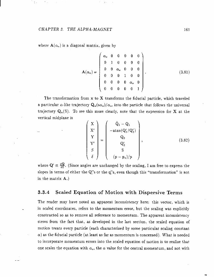
where A(a,) is a diagonal matrix, given by
/ a* 0 0 0 0 0 \ 010000
,) = 0 0 a0 0 0 0
000100
0 0 0 0 a, 0
\ 000001 )
(3.81)
- The transformat,ion from x to X transforms the fiducial part.icle, which traveled
a particular a-like t,raject,ory Qa(saO)/ a,, into the particle that, follows the universal
traject,ory Q,(S). To see this more clearly, note t,hat, the expression for X at, the
vertical midplane is
X
X’
Y
Y’
S
s
=
& - &I
-atan(Ql,lQ;) Q3
Qb
S
(P - PJP
(3.82)
where Q’ E g. (Since angles are unchanged by the scaling, I am free to express the
slopes in t,erms of either the Qf’s or the qi’s, even though this “transformation” is not,
in the mat,rix A.)
3.3.4 Scaled Equation of Motion with Dispersive Terms
The reader may have noted an apparent inconsistency here: this vector, which is
in scaled coordinat,es, refers to the momentum error, but the scaling was explicit,ly
constructed so as to remove all reference to momentum. The apparent inconsist’ency
stems from the fact that, as developed in the last section, t.he scaled equation of
motion treats every particle (each characterized by some particular scaling constant.
o) as t.he fiducial particle (at least. as far as momentum is concerned). What. is needed
to incorporat,e momentum errors into the scaled equation of motion is to realize t.hat,
one scales bhe equation wit.h aO, the CL value for t,he central momentsum, and not, wit,h

CHAPTER 3. THE ALPHA-MAGNET 162
the particular o of every particle under consideration. The result.anb scaled equation,
wit.h dispersive effects included exactly, is
Q’l = - &Q’ x B(;l;
1 dQ = -~-&Q3,09Q1)
(3.83)
(3.84)
As foreshadowed at’ the end of the last, section, it, is not. entirely necessary t,o include
dispersive effects in this fashion. One can obtain all dispersive terms in the matrices
by taking derivat.ives wit.h respect, t,o S after revert,ing t,o unscaled coordinat,es, though
this requires some care if it, is to be done correctly. This will be discussed in more
detail below. One reason for inserting dispersive effects at, this point? is t.o retmain t’he
six-dimensional transport matrix formalism. Anot’her reason, as indicat,ed at’ the end
of the last, section and as will become more apparent’ below, is that putting dispersive
effects into the formalism provides a check on t.he calculation of the matrix.
3.3.5 Scaling of the Transport Matrices
One can define transformation matrices for the vector X, with the realization that’
these transformation matrices apply to the scaled form of the equation of motion:
XI _+ G + C RIJXJ + C TwKXJXK + C UIJKLXJXKXL. (3.85) I J/K J>K>L
If I now substitut.e into this relation t.he definit,ion of X, equation (3.80), I obt,ain
c AISL - G + C RIJ AJjxj + C C TIJK AJjxj AKkXk + m Jj J/K jk
cc UHKLAJjXj AKkXk ALlXl- J>K/L jkl
Multiplying from t,he left by A,’ and summing over I yields
Xi + CA$‘CI $ CA~~RIJAJ~X~ $ C C A,lTIJKAJjXjAKkXkS I Uj J>K Ijk
C C A,1UIJKLAJjXj-4KkXkALlXl. J>K>L Ijkl
(3.86)
(3.87)
(3.88)
CHAPTER3. THEALPHA-MAGNET 163
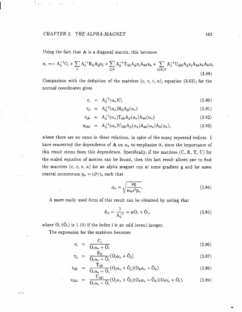
Using t,he fact. that, A is a diagonal matrix, this becomes
Xi - Aii’Ci + C A,lR..A*. u DXj $ C Ai~*TijkA~XjA~Xk + C A1~‘U~~A~XjA~XkA~Xl. j j/k j>k>l
(3.89)
Comparison wit,h the definition of the makices (c, r, t, u), equation (3.63), for the
normal coordinates gives
Ci = A,r( a,)Ci (3.90)
rij = A,:‘( ct:,)RtiAji( a,) (3.91)
tijk = &l(Ct.o)‘JJijkAz( ao)Ati( ao) (3.92)
Uijkl = A,l(a,)UijMAji(a,)Akk(a,)An(~:,), (3.93)
where there are no sums in t,hese relations, in spit,e of the many repeakd indices. I
have reasserted the dependence of A on a, to emphasize it, since the importance of
this result stems from this dependence. Specifically, if the matrices (C, R, T, U) for
the scaled equat,ion of motion can be found, t,hen t.his last result, allows one to find
the matrices (c, r, t, u) for an alpha magnet’ run at’ some gradient. g and for some
central momemum p0 = (Pr)O such t.hat
eg CL&= - J mec2Po ’
A more easily used form of this result. can be obt.ained by noting t,hat#
Aii = 1 = Ai;l
CuOi + Oiy
where Oi (Oi) is 1 (0) if the index i is an odd (even) integer.
The expression for the matrices becomes
Ci Ci =
OiOLc, + 0;
r.. = u
t ijk = oia + 0. (Ojao + oj)(OkQo + Ok)
lliju = o,fiT 01 (Oj% $ Oj)(okQ, $ Ok)(o1a, $ 01). 1 0 1
(3.94)
(3.95)
(3.96)
(3.97)
(3.98)
(3.99)
-
CHAPTER3. THEALPHA-MAGNET 164
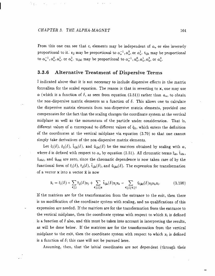
From this one can see that, ci elements may be independent, of a, or else inversely
proport,ional to it. rij may be proportional to oil, cri, or ai. tijk may be proportional
to Q;~,c.$,Q:, or a:. UGM may be proportional t.o ai’, cwt, ai, a:, or cr:.
3.3.6 Alternative Treatment of Dispersive Terms
I indicated above t,hat it is not necessary to include dispersive effects in the mat,rix
formalism for the scaled equation. The reason is that. in reverting t,o x, one may use
a (which is a function of S, as seen from equation (3.51)) rather than o,, t.o obtain
the non-dispersive matrix elements as a function of 6. This allows one to calculate
the dispersive matrix elements from non-dispersive matrix elements, provided one
compensat’es for the fact, that. the scaling changes the co0rdinat.e system at, the vertical
midplane as well as t,he moment.um of the particle under consideration. That is,
different, values of a correspond to different. values of qi, which enters the definition
of the coordinates at the vertical midplane via equation (3.70) so that. one cannot,
simply t,ake derivatives of the non-dispersive matrix element,s.
Let E;(S), f,(h), tijk(s), and iiijM(S) be the mat’rices obtained by scaling with a,
where 6 is defined with respect, to Q, by equation (3.51). All chromatic terms i!iG, ii6k,
5;6u, and iii661 are zero, since the chromatic dependence is now taken care of by the
functional form of E;(S), rij(S), f:ijk(b), and iiij~(S)+ The expression for transformation
of a vect,or x into a vector f is now
Xi = Ei(S) $ C fij(S)Xj $ C iijk(fi)xjxk + C fiijkl(~)xjxkxl* (3.100) 43 4>j/k 4>j>k>l -- -
If the matrices are for bhe transformation from the entrance to the exit, then there
is no modification of the coordinate syst’em wit’h scaling, and no qualifications of t,his
expression are needed. If the mat.rices are for the transformat,ion from the ent,rance t,o
the vertical midplane, then the coordinate system with respect to which %i is defined
is a function of S also, and this must be taken into account, in interpreting the result.s,
as will be done below. If the matrices are for the transformat,ion from the vertical
midplane to 6he exit,, then t,he coordinat,e system with respect. to which x; is defined
is a funct.ion of 6; this case will not. be pursued here.
Assuming, t,hen, that. t.he initial coordinates are not dependent (through t,heir
.
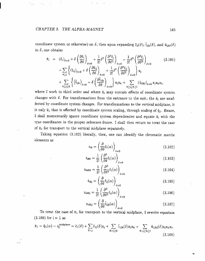
CHAPTERS. THEALPHA-MAGNET 165
coordinate system or obherwise) on S, then upon expanding Iij(S), iijk( S), and UijH(S)
in S, one obtains
xjxk + c (fiijkl)6=OXjXkXI,
where I work t,o t,hird order and where xi may con&in effects of coordinade system
changes with 6. For transformations from the entrance to the exit., the Xi are unaf-
fect,ed by coordinate syst,em changes. For transformations to the vertical midplane, it,
is only xr that. is affected by coordinat*e system scaling, through scaling of qr. Hence,
I shall momentarily ignore coordinat,e system dependencies and equat,e xi with the
true coordinates in the proper reference frame. I shah then ret,urn to t.reat. the case
of ztl for transport to the vert,ical midplane separately.
Taking equation (3.102) literally, t,hen, one can identify the chromatic mat,rix
elements as
(3.102)
(3.103)
(3.104)
(3.105)
(3.106)
(3.107)
To treat, the case of fi for transport to t.he vertical midplane, I rewrit,e equation
(3.100) for i = 1 as
21 = &(a) - qydpl- = El(b) + ~~lj(fi)xj + c f:ljk(b)XjXk + c ~ljkl(~)XjXkX1, S>j 6>j>k 6>j>k>l
(3.108)
.
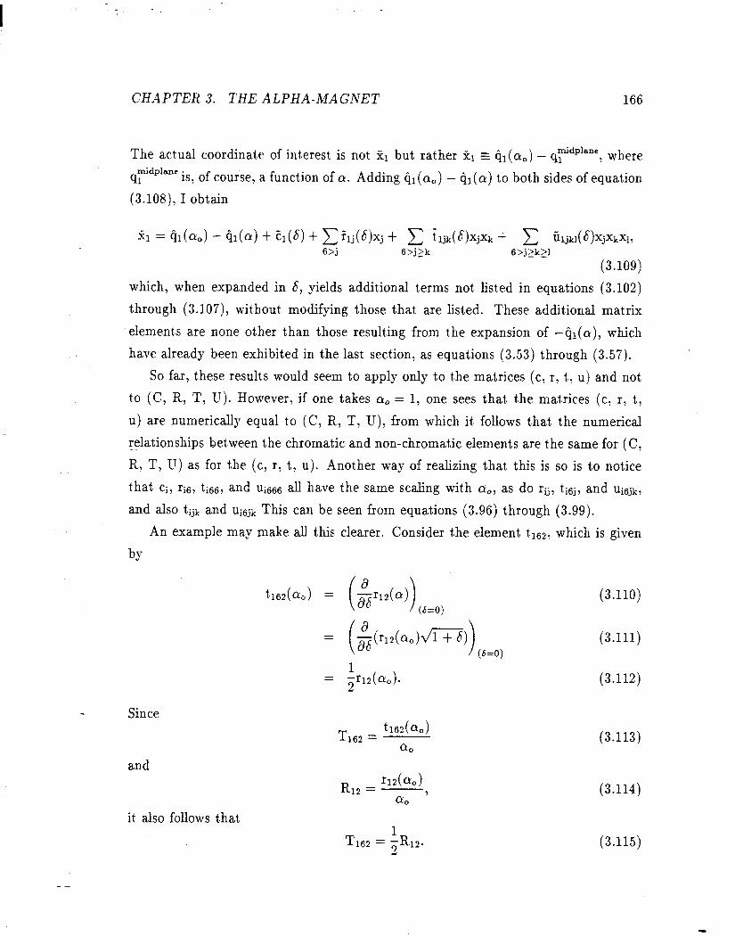
CHAPTER3. THEALPHA-MAGhTET 166
The act,ual coordinat,e of int,erest is not, ~1 but, rather xl 5 ql( a,) - qydplane, where midplane .
91 is, of course, a function of cr. Adding qi(aO) - &((Y) to both sides of equat,ion
(3.108), I obtain
21 = 41 (Cl!,) - &(a) $ cl(b) $ c ?lj(b)Xj + c iljk( b)xjxk + c ~ljkl(~)xjxkxl, S>.i S>j>k 6>j>k/l
(3.109)
which, when expanded in S, yields addit,ional terms not, listed in equations (3.102)
through (3.107), wit,hout, modifying those that are listed. These additional matrix
elements are none other than those resulting from the expansion of -&(a), which
have already been exhibit,ed in the last section, as equations (3.53) through (3.57).
So far, these results would seem to apply only to t.he matrices (c, r, t., u) and not,
to (C, R, T, U). However, if one takes a0 = 1, one sees that, the mahrices (c, r, t,
u) are numerically equal t,o (C, R, T, U), f rom which it. follows that’ the numerical
relat,ionships between the chromatic and non-chromatic elements are the same for (C,
R, T, U) as for the (c, r, t, u). Anot’her way of realizing that this is so is to not.ice
t#hat, Ci, ris, tic69 and ui666 all have t,he Same SCahg wit’h a,, 8S do rij, ti6j, and Ui6jk,
and also t,ijk and Ui6jk This can be seen from equations (3.96) through (3.99).
An example may make all this clearer. Consider t,he element t,i62, which is given
bY
Since
and
h62(%) =
T t162(%)
162 = a0
n2b) R12 = -
a3 ’
it, also follows t.hat,
T 12.
(3.110)
(3.111)
(3.112)
(3.113)
(3.114)
(3.115)
--

.
C'HAPTER3. THEALPHA-MAGNET 167
For rapid checks on calculat,ed matrices, or for inclusion in a comput,er program,
it, is convenient t#o work out. the consequences of these relations for the matrices (C,
R, T, U). I have done this, and the result,s are
1 R56 = 45,
2
1 T566 = -45,
8
U 5666 = 35’
and
TIGJ = $RIJ(OIOJ - OIOJ),
UI~~J = ~RIJ(~&OJ - O&J),
(3.116)
(3.11i)
(3.118)
(3.119)
(3.120)
. . UIGJK = IJE; [o@J& - OIOJOE; - o,(oJ& + OJOK) - 2bI0J04, (3.121)
where 01 (01) is 1 if I is odd (even) and zero’ ot,herwise, and where 6 > J 2 K. (I
emphasize again that. these results are invalid for transport, from the vertical midplane
to the exit, which is a case I have not treated here.)

-. .
CHAPTERS. THEALPHA-MAGNET 168
3.4 Transport Matrices from Numerical Integra-
tion
The scaled transport. mat,rices (C, R, T, U) for the alpha-magnet, can be found from
numerical integration of the scaled equation of motion (equation (3.83)) and fitSting.
The technique I have used is not. confined in its application to the alpha-magnet,
though it, is most. appropriate for elements for which there exists an equivalent of
the scaled equat.ion of motion for the alpha magnet. Essentially, an ensemble of N
init,ial vecbors, labeled Xc’), i = 1,2,. . . N is mapped int.o an ensemble of final vect,ors,
labeled Y(‘), by numerical integrat.ion starting and ending at the appropriat,e reference
planes. These vectors are t,hen required to satisfy
Yii’ = CI + c RrJX:‘) + c TIJKXy)X;) + c UUKLXF)X;)Xt)+ J JZK J>K>L
c vUKLMx~$$)X~)xfJ + q(xCi))5) , (3.122)
which is essentially the definition of the transport’ matrices, where I’ve included a
fourth-order matrix V. I emphasize that. the Yci) are not, calculated from this ma-
trix expression, but are rather being approximat,ed by it,, having been calculated by
numerical int,egration of the equation of motion with initial condition Xc’). I am in-
cluding t,he fourt,h-order terms explicitly in order t,o show how to prevent, fourth-order
influences from corrupting t.he computat,ion of (C, R, T, U). The fifth-order t,erms
will be assumed to be negligible.
3.4.1 One-Variable Terms
In principle, one could fit this by finding the (C, R, T, U) that minimized the sum
of t,he squared deviations of the right-hand-side from the left.-hand-side. In practice,
t,his is compudationally difficult and also extremely inefficient. To see a more efficient,
procedure, imagine that, one was only interesbed in calculat,ing Cr. Clearly, one would
only need t.o track the fiducial particle.
At, firsts sight,, one might think that, one could then go on t,o find Ru by finding
Y for each vector of an ensemble, XcJ), of init,ial vectors, each of which had only a
--

CHAPTER3. THEALPHA-MAGNET 169
non-zero Jth component:
xtJ) = aJeJ, (3.123)
with J = 1.. .6, aJ a constant, and eJ t,he unit vector for the Jth component8 of X. In
fact, the YiJ’ values thus obtained would include the influence of not only RIJ, but
also of all non-zero TIJJ, U~JJ, and VLJJJJ matrix elements:
$’ = CI + h.JaJ + TIJJil; + UIJJJai + VIJJJJai + o($). (3.124)
Obviously, one can extract. C I, IJ, R T IJJ, and UIJJJ by fit,ting a fourth-order poly-
nomial t#o this form (assuming that, terms of fifth-order and higher can be ignored),
if one takes a sufficient, number of values of aJ for each J. A minimum of five initial
vectors are needed for each value of J. Since I consider only static systems, J=5 (i.e.,
path-length dependent) t$erms are all zero, so a minimum of t,went,y-five vectors needs
t,o be integrated. As I will discuss below, I use N vectors per component. J, with N
Cidd and N 2 5:
xcJi) = (j - F)aJeJ, j = 1...5. (3.125)
The reason for this particular choice of XcJj), which is symmetric about. and includes
the origin, will become apparent below. aJ is chosen sufficiently small so as to avoid
large contributions t,o Y from terms higher than fift.h order, while obtaining reasonable
influence from third order terms, so that, fit.ting will yield sufficiently precise values
for the third-order coefficients. This st.ep gives all elements Cr, RIJ, TIJJ, UIJJJ, and,
as a useful bonus, VIJJJJ. It remains to find T IJK = TIKJ, UIJKK = UIKJK = UIKKJ,
and UIJKL, for J > K and K > L.
3.4.2 Two-Variable Terms
To find TIJK and UIJKK, I integrat*e the equations of motion for a new ensemble of
initial vectors for each (J, K) pair with J > K, described by
XcJitKTk) = (j - F)aJeJ $ (-l)kaI<eK, (3.126)
where j = 1. . . N, k = 1 or 2, N is an odd integer, and aJ and aK are constants.
I now construct, a residual final vector, AY(Jj~K~k) for each X(Ji9K*k) by subtract,ing
off the contributions of the known matrix elements.
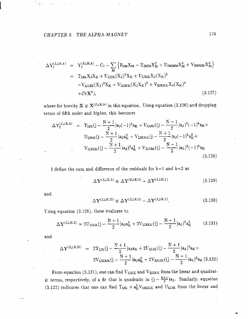
CHAPTER 3. THE ALPHA-MAGNET 170
AY(Ji’K*k) I = Y~Ji’K’k) - CI - C {R~MXM + TIMMX& + UrMMMXL + VrMMMX&} M
= TIJKXJXK + UIJJK(XJ)~XK + UIJKKXJ(XK)~
+VIJJJK(XJ)~XK + VIJJKK(XJXK)~ + VIJKKKXJ(XK)~
+0(X5>, (3.127)
where for brevit.y X - X (J,j*Ktk) in this equation. Using equation (3.126) and dropping
terms of fift.h order and higher, this becomes
Ay’Jj,“,k) I = Tm(j -
N+l T)aJ(-l)kaK •t UIJJK((j - y)aJ)2(-l)kaK+
N+l UIJKK(j - -
2 ) aJ& + VIJKKE;(~ -
N+l F)aJ(-l)kai-+
VIJJKK((j - y)aJ)2ai $ VIJJJK((j - y)aJ)3(-ll)kaK
(3.128)
I define the sum and difference of the residuals for k=l and k=2 as
Ay(Ji,K,S) E Ay(J,j,K,2) + ~y(Ji,Kl) (3.129)
and ~y(JtiW) E ~y(Ji,K,2) _ ~y(Ji,K,l).
Using equabion (3.128), these evaluat(e t,o
(3.130)
N+l A~(J~~K*S) = 2UIJKK(j - - 2 )
aJai + zVIJJKK((j - (3.131)
and
N+l AY(J’j,K.D) = 2TrJI<(j - y)aJ&K + 2uIJJI<((j - F)aJ)‘aK+
zVIJKKK(j - N+l
2 ) aJ$ + sVIJJJK((j - y)a,J)3aK (3.132)
From equation (3.131), one can find U IJKK and v1J.r~~; from the linear and quadrat’-
ic t,erms, respect,iveIy, of a fit that. is quadrat.ic in (j - ?)a,. Similarly, equat’ion
(3.132) indicates t,hat one can find TIJK $ &VIJKKK and UZJJK from the linear and

I :
CHAPTER 3. THE ALPHA-MAGNET 171
quadrat,ic terms of a. fit. t,hat. is cubic in (j - y)aJ. By doing t,he analysis for two
different. VdUeS Of afi, one can Separate TIJK from TIJE; $ a;VIJKKK. For a general
element, then, at, the very least, one needs bwent.y int,egrations (i.e., N=5, t.wo values
of ae, j=1,2) for every pair (J, K), for J > K, or 20 * 15 = 300 integrations. (The
t.wenty is the number of int,egrations per pair; the fift,een is the number of (J, K) pairs
such that. 6 2 J > K 2 1.) Since the elements with J=5 or K=5 are known before-
hand to be zero for a st,at,ic element., this is reduced to a minimum of 20 * 10 = 200
int’egrat’ions for the alpha-magnet.
3.4.3 Three-Variable Terms
Having complebed t.his st.ep, only the elements U IJKL with J > K and K > L remain
to be found. To obt.ain these, new init,ial vect,ors are chosen for each t.riplet, (J, K, L)
with J > K > L: . . x(JLLi) = (-l)i(
aJeJ •t aKeK + aLeL), (3.133)
where i is 1 or 2, and aJ, aK, and aL are constant’s,
Again, I comput,e residual final vectors AY (J,KvL,i) bv subt.ract,ing off the contri- v
butions of all R: T, and U matrix elements calculated so far:
Ay(JtK7Lti) f y I $J’K’L’i) - CI - 1 { RINXN + T INNXi + UINNNXi + VINNNNX~
N - c( TINMXNXM + (UINMMXN(XM)~ + U INNdxN)2xM)}
N>M
= c UINMPXNXMXP + c hNNMM(XNXM)2
N>M>P N>M
+ 1 (VINMPPXNXMX; + VINMMPXNXCXP + VINNMPx$MXP}
N>M>P
+Q(X5), (3.134)
where for brevit.y X zz X(J*K,L9i) in this equation. Using equation (3.133) and dropping
terms of fift.h order and higher, this becomes
AYii’ = UIJr;LaJaKaL(-I)‘$
(VIJJKKajak -t VIJJLLaiat + vIKKLL&af,)+
(vIJKLLa,JaKat + 12VIJKKI,aJ&a~ + VIJJKLa~aKaL). (3.135)

CHAPTER3. THEALPHA-MAGNET 172
I now form the difference of t.he residuals for i=2 and i=l, obt.aining
AYCD) 1 YC2) - Y(i) = 2UIJKLaJaKaL. I - I I (3.136)
Thus, one can obtain the UIJKL with J > K and K > L by integrating a two additional
vectors for each triplet. J > K > L, requiring 40 additional integrations for a general
element. For a stat#ic element, UIJKL = 0 for J=5, K=5, or L=5, which reduces the
number of addit,ional int#egrations to 20.
3.4.4 Initial-Vector Ensemble . .
The reader may have noticed that, the ensembles specified by equations (3.125),
(3.126), and (3.133) overlap. Because of t,his, it. is possible to use the ensemble
of vectors defined by
x(J,iKkL1! = (NJ ’ ’ _ j)aJeJ + ( NK ’ ’ - k)arCeh: + ( NL + 1
. . 2 2 - - l)aLeL, (3.137) 2
wit.h NJ odd, 6 > J > K > L > 1, and j, k, and 1 taking integer values bet,ween
-(N - 1)/2 and (N - 1)/2 ( w h ere N = NJ, NK, or Nr,, for j, k, and 1, respective-
ly) except that, j = k = 1 = 0 (the null vector) appears only once for all triplets (J, K,
L). The maximum amplit,ude of the Jth vector component, is
MJ = NJ - 1 -aJ.
2 (3.138)
Since for a static element,, X5 is irrelevant, one can choose N5 = 1 and $5 = 0. It.
is also convenient. to choose NJ = N for all J # 5. Given bot,h of these choices, the
number of vect#ors in the ensemble is
10(N3 - 1) + 10(N2 - 1) + 1, (3.139)
where I count ten (J, K, L) triplets with neit,her J, K, nor L equal to 5, contributing
N3 - 1 vectors each, exclusive of the null vector; ten (J, K, L) triplets with one of J,
K, or L equal t#o 5, contributing N2 - 1 vectors each, exclusive of the null vector; plus
one null vector.
For N = 5 t.his ensemble contains about. 6 times as many vectors as the minimum
needed, but’ using it, has t,he advantage of simplicit,y of coding and also of provid-
ing additional dat,a t,o improve the accuracy of some of the element,s by averaging.

CHAPTER3. THEALPHA-MAGNET 173
Doubtless a more computat,ionally efficient. ensemble could be coded t,han I have used
in my codes.
Having assembled this ensemble, one integrates each initial vector to obt,ain the
corresponding final vect,or. One then selects out, the necessary sub-ensembles corres-
ponding to equat,ion (3.125), (3.126), or (3.133)) for each stage of the analysis.
3.4.5 Accuracy Considerations and Limits
I have taken pains in the above analysis to eliminat,e the influence of fourth-order
terms in order to-increase the accuracy of the third-order matrix. In addition, suitable
choice of the const.ants 8J can ensure that, t.he effects of fourth and higher-order t.erms
are negligible. “Suit,able” must’ be determined empirically, or by reference to t.he
magnitude of the mat’rix elements once they are roughly known. A starting point is
to assume that’ the dominant, fourth-order matrix elements have magnitudes similar to
those of dominant’ matrix elements of third-order, from which one would conclude that,
t.hat# MJ = 10v3 would be suit,able to obtain 0.1% accuracy of the third-order results,
even wit,hout, the corrections for the V matrix that. are included in the equations.
Furt,her, fifth order terms would be expect,ed have an influence of one part’ in a
million relative to the third-order. If similar results are obtained for a wide range
of values of MJ, bhen one can conclude that the influence of higher-order t’erms is
indeed negligible. In addiCon, if the contributions of t,he first, second, and t,hird-
order matsrices to the final coordinates Y are seen t,o be different. by several orders of
magnitude between successive orders, then one can reasonably conclude that. higher-
order effects are several orders of magnitude below the third-order effects.
Invariably the above procedure will yield some small, non-zero matrix element,s
which may or may not. be genuine, due t.o the accumulation of inaccuracies in the
integraCon, subtraction of higher-order terms, and fitt(ing. If one knows that the
accuracy of any integration is of order 10mp, where p is an integer, then one can con-
clude that a computed mat,rix element is spurious if it fails to satisfy the appropriat,e
criterion (depending on t#he order of the matrix element,) from the following list:
RIJMJ > lo-* (3.140)
TLIKMJMK > lo-* (3.141)
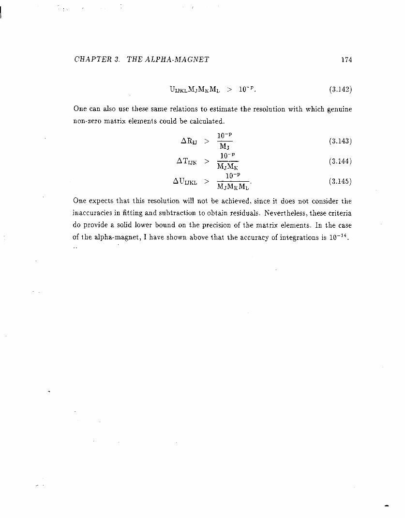
CHAPTER3. THEALPHA-MAGNET 174
UIJKLMJMKML > IO-‘. (3.142)
One can also use t,hese same relations bo est,imat#e the resolution with which genuine
non-zero matrix elements could be calculat.ed.
10-p ARIJ > -
MJ
10-p ATUK > -
MJMK
AUIJKL > 10-P
MJMKML
(3.143)
(3.144)
(3.145)
One expects that. this resolut,ion will not, be achieved, since it. does not consider t.he
inaccuracies in fitting and subtraction to obt,ain residuals. Nevertheless, t,hese criteria
do provide a solid lower bound on t.he precision of t.he matrix elements. In the case
of t,he alpha-magnet, I have shown above t#hat’ the accuracy of int,egrations is 10-14.
CHAPTER 3. THE ALPHA-MAGNET 175
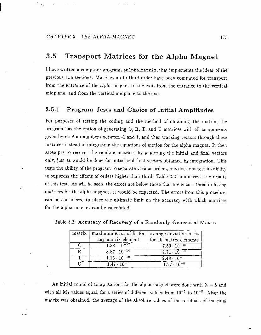
3.5 Transport Matrices for the Alpha Magnet
I have writt,en a computer program, salphamatrix, t,hat’ implements the ideas of t.he
previous two sections. Matrices up to third order have been computed for transport
from t.he entrance of t,he alpha-magnet, to the exit, from the ent,rance to the vertical
midplane, and from the vertical midplane to the exit.
3.5.1 Program Tests and Choice of Initial Amplitudes
For purposes of testing t’he coding and t.he met,hod of obtaining the mat,rix, t.he
program has the opt.ion of generating C, R, T, and U matrices with all component’s
given by random numbers bet,ween -1 and 1, and then tracking vect,ors through t,hese
madrices instead of integrat,ing the equations of motion for the alpha magnet. It t,hen
attempts to recover t*he random mat,rices by analyzing t.he initial and final vect,ors
only, just as would be done for initial and final vect.ors obt,ained by int’egration. This
t,ests the abilit,y of the program to separat.e various orders, but, does not. t.est its ability
to suppress the effects of orders higher t,han t.hird. Table 3.2 summarizes the result,s
of this test.. As will be seen, the errors are below t.hose that. are encount,ered in fit,ting
matrices for the alpha-magnet, as would be expectSed. The errors from this procedure
can be considered t’o place the ultimat,e limit. on t,he accuracy wit.h which matrices
for t.he alpha-magnet, can be calculat,ed.
Table 3.2: Accuracy of Recovery of a Randomly Generated Matrix
matrix maximum error of fit’ for average deviat,ion of fit any mat,rix element, for all matrix element,s
C 1.38 . lo-l7 7.59 * lo-‘”
R 8.87 - lo-l4 2.71 - lo-l4 T 1.13 * lo-lo 2.48 . 10-l’ U 1.47 * 1o-i 1.77 - 10-s
An initial round of computations for the alpha-magnet were done wit.h N = 5 and
wit,11 all MJ values equal, for a series of different’ values from 10m2 to 10m5. After t,he
matrix was obtained, the average of the absolute values of the residuals of the final
--

CHAPTERS. THEALPHA-MAGNET 176
vect,ors for all initial vectors were comput,ed to assess the degree t#o which the fit,s
contained sufficiently high-order t,erms to match the act,ual final vectors. Residuals
were comput,ed by successively adding linear, second-order, and third-order terms t,o
assess the effect of each order. The average absolute residuals for nth order are simply
@“’ = l Mi
II 1
Jy _ Cl + ~R~JXY) + (n > l?) c TIJE;X~)X$)+ (3.146) J J>K
(n > 2?) C U~E;LX~‘)X~)X~’
)I
, (3.147) J>K>L
where the index i runs over all M initial vect,ors in the ensemble specified by equation
(3.137), and (n > m?) represent,s a function 6hat. returns 1 if n > m and 0 otherwise.
Table 3.3 summarizes some of the results. (Rf) is identically zero, since the momen-
tum is not, changed by the magnet., and hence is not, listed.) It’ is no coincidence that’
for any particular I and n, Rp) varies with MJ according to MJ”‘l, since for valid fit’s
(i.e., those t’hat, don’t. err by compromising lower order coefficients in order to mat.ch
higher-order contributions) RI”’ is simply the average cont’ribution of t,he (n + l)th
order t,erms.
Table 3.3: Residuals from Matrix Fits
n MJ $4
1.84 .11O-3 w RF) w w
1 1o-2 1.89. 1O-3 4.51 * 1o-4 3.79 * 1o-4 7.63 - 1O-5
1 1o-3 1.84 . 1O-5 1.89 . 1O-5 4.49 * 1o-6 3.53 - lo+ 7.76 - 1O-7
1 1o-4 1.84. 1O-7 1.90 * 10-i 4.49 - 1o-s 3.51 . 1o-s 7.76 . 1O-g
2 1o-2 3.44 * 1o-5 2.39 . 10-5 4.59 - 1o-5 1.43 * 1o-4 6.38 - 1O-6
2 1o-3 3.44 * 10-s 2.39 * 10-s 4.61 . lo-” 1.43 . 1o-7 6.34 . 1O-g 2 1o-4 3.44 . 10-l’ 2.39 e lo-l1 4.61 . lo-l1 1.42 . lo--lo 6.34. lo-l2
3 1o-2 9.40 * lo-’ 8.78 - 1O-7 2.08 . 1O-6 2.37. 1O-6 7.19 * 10-7 3 1o-3 8.98 . lo-l1 8.43 . 10-l’ 2.08 . lo-lo 2.36 . lo-lo 7.21 . lo-l1 3 1o-4 1.14 . lo-l4 1.01 s lo-l4 2.07. lo-l4 2.36 . lo-l4 7.40 - lo-l5
Table 3.3 shows that, for MJ = 10H4, the third-order residuals are of order 10-14,
which is the accuracy limit, of the int,egrations. Hence, fourt*h-order corkibutions are
?n the noise”: and third-order contributions are three orders of magnit,ude above it,. I
find t,hat’ for such small hlJ values, the chromadic terms do not follow equations (3.102)

CHAPTER3. THEALPHA-MAGNET 177
through (3.107) as well as for MJ = 10e3. For this reason, I choose the matrices
compuhed wit,11 MJ = 10e3 as the most’ accurate. Analysis of the chromatic t,erms
indicates that, the T matrix elements are accurat,e to about’ 10e6, indicat.ing that’ p in
equations (3.143) t,hrough (3.145) is 12 (rather than 14 as would be thought, from t,he
accuracy of the integration). I use this value of p in order t,o “filter” small TIJK and
UIJKL values for significance, as per equations (3.140) through (3.142). That, is, TIJK
values smaller than low6 and U IJKL values smaller than 10m3 are taken to be zero.
3.5.2 Final Results
Having verified the program’s matrix-fitting algorithm and found the limits of its
accuracy, I computed the mat’rices for the alpha magnet, using N = 7. I used an
accuracy limit. of 5 x lo-l3 to filter out spurious non-zero matrix elements. This limit
is a compromise bet,ween one that, is somewhat too large for t,he T matrix elements,
and somewhat’ too small for the U matrix elements. Hence, some small, dubious U
matrix elements will appear in t.he results t,hat follow.
Checks of the Results
A number of checks have been made on t.hese matrices. The determinams of t,he
first. order mat.rices for entrance-to-exit, emrance-t,o-vert’ical midplane, and vert,ical
midplane-to-exit have been found t.o be 1 to wit’hin 2 x 10-12. (This accuracy is not’
fully reflect.ed in t.he resuhs given below, since I have not. quot,ed a sufficient’ number
of significant, figures. Also, t.he reader should beware of checking this claim wit,h a
hand calculatSor, since many use only 10 or 11 digits.)
The relationships between the non-chromatic and chromaCc terms were used t,o
evaluate the accuracy of the method, as discussed above; the reader is invited to
use equations (3.102) t.hrough (3.107) and (3.53) through (3.60) t,o verify for himself
-that the results do indeed satisfy the expected numerical ratios. As a sample, for the
matrix .from the ent,rance to the vertical midplane, I find t,hat
R56 -= c5
f + 2 * lo--l2
T566 1 - = _- _ 6. 1()-1o
c5 8
(3.148)
(3.149)
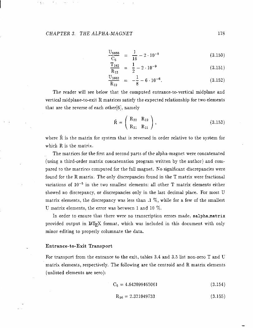
CHAPTERS. THEALPHA-MAGNET 178
u5666 1 - = -- (35 16
2 - 1o-8
T 162 1 -= R12
- - 2 .1()-g 2
(3.150)
(3.151)
U 1662 1 - = --- R12 8
6 . lo-? (3.152)
The reader will see below that the computed entrance-to-vertical midplane and
vertical midplane-t.o-exit’ R matrices satisfy the expected relationship for two elements
t,hat, are the reverse of each ot’her[6], namely
R= (3.153)
where I? is the matrix for syst,em that is reversed in order relative t.o the system for
which R is the makix.
_- The mat’rices for the first, and second parts of the alpha-magnet, were concat’enated
(using a third-order matrix concat,enat,ion program writ,ten by t,he aut,hor) and com-
pared t#o 6he matrices comput.ed for t.he full magnet. No significant, discrepancies were
found for the R matrix. The only discrepancies found in the T matrix were fractional
variations of 10e5 in the t,wo smallest, elemems; all ot,her T matrix e1ement.s eit,her
showed no discrepancy, or discrepancies only in the last decimal place. For most. U
mat,rix elements, t,he discrepancy was less than .l %, while for a few of the smallest’
U matrix elements, the error was between 1 and 10 %.
In order t,o ensure that. there were no transcript,ion errors made, salphamatrix
provided output, in I~TEX format, which was included in this document’ widh only
minor editing to properly co1umnat.e the data.
Entrance-to-Exit Transport
For transport, from the entrance to t.he exit, tables 3.4 and 3.5 list non-zero T and U
makix elements, respectively. The following are the cenkoid and R matrix elements
(unlist(ed elements are zero):
C5 = 4.642099465061
R56 = 2.321049T33
(3.154)
(3.155)

: .
CHAPTERS. THEALPHA-MAGNET 179
(3.156)
( ;;; I%:; ) = ( -0.7371140937 7.618204274 )
-0.05994362928 -0.7371140937 (3.157)
Table 3.4: Non-zero T Matrix Elements from Entrance to Exit
TIz2 = -9.985582.10-l T133 = -6.047097.10-’ T1d3 = -6.415746 T144 = 3.782911. lo1 Tl‘j2 = -1.160525 T233 = -2.996743. lo-’ T243 = -7.370063 T244 = 3.808545. lo1 T331 = -5.157770. 1O-2
T332 = 9.264364 T342 = 6.892273 T364 = 3.809102
T432 = -1.750135 T441 = 5.157770. 1O-2 T442 = 9.384079 T463 = 2.997181. lO-2 Tsz2 = 5.802624 -10-l T533 = 1.104632. 1O-2
T543 = -2.283314.10-l T544 = -1.403871 T566 = -5.802624.10-l
Table 3.5: Non-zero U Matrix Elements from Entrance to Exit
U1222 = 9.634. 10-l
u1431 = -5.301
IT1442 = 9.435 ’ lo1
111644 = 1.891. lo1
U2431 = 5.157’ lo-’
Ur,,,, = 4.557 ’ lo’
Us321 = -1.462
113411 = 4.431. 10-2
U3432 = -2.705. lo-3
U3444 = -1.075. lo2
us664 = -9.523 ’ lo-’
U4421 = 1.463
u4433 = -1.441
U4632 = 8.751. lo-’
115222 = 4.993.10-l
U5431 = 1.873 1 1O-2
Us442 = -2.145. lo’
tT5644 = -7.019 * 10-l
u1331 = -2.579. 10-l
U1432 = 8.263. 10’
tTl622 = -4.993 * lo-’
ul&j2 = 2.901 * lo-’
u2432 = 9.310 ’ lo’
172633 = 2.99-i ’ 10-l
u3322 = -4.979 ’ lo-’
U3421 = 1.033. lo-’
U3433 = -2.310
u3631 = 2.579 * lo-2
U4322 = 1.285. lo’
u4422 = 2.946
u4443 = 8.688.10’
U4641 = -2.575. lo-2
U5331 = 1.546. 1O-3
Us432 = -4.126. 10-l
u5622 = 2.901. 10-l
u,,,, = 2.901.10-
U1332 = -8.573
U1441 = 3.829. 10’
U1633 = 3.023. 10-l
IT2332 = -8.779
U2441 = 6.341
U2,j43 = 3.685
113333 = 1.047
173422 = 1.101 ’ lo1
u3443 = 2.220.10’
U3642 = 3.446
U4333 = -4.323. 10-l
U4432 = -1.636. lo-3
U4444 = -3.156. lo2
U&j63 = -2.248. lo-2
us332 = 2.469 ’ lo-2
IT5441 = 9.242. 1o-4
Us633 = -5.524. lo-3

CH.4PTER 3. THE ALPHA-MAGNET 180
Entrance-to-Midplane Transport
For t,ransport from the entrance to the vertical midplane, tables 3.6 and 3.7 list non-
zero T and U matrix elements, respectively. The following are the cent*roid and R
matrix element#s (unlisted elements are zero):
c5 = 2.321049732530 (3.158)
R51 = -2.179660432 (3.159)
R52 = -2.529550131 (3.160)
R16 = -9.089085575 -10-r (3.161)
R56 = 1.160524866 (3.162)
R66 = 1.000000000 (3.163)
0.07531765053 2.182639820
-0.3979387890 1.745181272 (3.165)
Table 3.6: Non-zero T Matrix Elements from Entrance to Vertical Midplane
Till = 1.581820 T121 = 3.671483
T133 = 3.170513.10-’ TIDE = -4.724714.10-l
T162 = 2.084977. lo-’ Tls6 = 2.272271.10-l
T222 = 1.835742 T233 = -3.739056. lo-’
T244 = 7.286366. lo-’ T261 = 1.199054
T332 = 3.240582 T341 = -2.367091
T364 = 1.091320 T431 = -9.936083 ’ 1O-2
T441 = -2.536989 T&Y = -2.015590
T521 = 1.875460 T522 = 1.378390
,T543 = 4.235456. 10-l T544 = 1.614540
T566 = -2.901312.10-1
Tlz2 = 2.357651
T144 = -2.932169.10-l
T221 = 2.613530
T243 = 9.437959 ’ 10-l
T331 = 5.249703.10-l
T 342 = -1.933840
T432 = 2.168953
T&j3 = 1.989694.10-l
T 533 = -3.473390.10-l
T562 = -1.264775

-
CHAPTERS. THEALPHA-MAGNET 181
Table 3.T: Non-zero U Matrix Elements from Entrance to Vertical Midplane
U1211 = -3.085 U1221 = -5.581 U122~ = -2.478 U1331 = 4.933.10-I U1332 = 3.610. 1o-2 U1431 = -1.791
U1432 = -2.841 IT1441 = -5.547. 10-l U1442 = -1.004 U1611 = -7.909.10-l tJ1622 = 1.179 U1633 = -1.585 ’ lo-’ tJ1644 = -1.466. lo-’ IT1662 = -5.213. 1o-2 U1666 = -1.136. lo-’
U2111 = -6.200 u2211 = -2.159.10’ U2221 = -2.700. 10’
U2222 = -9.493 tJ2331 = 2.284. lo-’ tJ2332 = 1.145
U2421 = -1.025. lo-’ U2431 = 1.686 U2432 = 1.572
U2441 = -4.851 tJ2442 = -4.688 U2621 = -1.307 CT2633 = 3.739. 10-l IT2643 = -4.719 10-l tJ2661 = -8.9%. 10-l
1J3311 = 6.554. 1O-2 tJ3321 = -3.313 tJ3322 = -4.769
U3333 = 3.965. 10-l u3411 = 1.448 tJ3421 = 1.908 u3422 = 3.934 ’ lo-’ u3433 = -1.195 U3443 = -8.190. 10-l
u3444 = 1.457 U3631 = -2.625. 10-l IT3642 = -9.669. lo-’
CT+4 = -2.728. 10-l U4311 = -3.463. 10-l u4321 = -4.190 LJ4322 = -4.777 U4333 = 2.704.10-l U4411 = 1.604 LJ4421 = 2.868 U4422 = 1.015 u4433 = -9.890.10-l u4443 = 1.350.10-’ U4444 = 5.265.10-l u+,j31 = 9.936. 1o-2
LJ,,,, = -1.084 tJ4641 = 1.268 u4663 = -1.492. lo-’
LJ5111 = -1.264 tJ5211 = -4.402 U522l = -7.153 LJ5222 = -2.112 U5331 = -1.045 * 10-l tJ5332 = 1.548. 10-l
u5431 = 1.514 r-J5432 = 3.542 u5441 = -2.804
35442 = -1.689 U5622 = 6.892.10-l Us633 = 1.737. 10-l J5644 = 8.073 ’ 10-l Usss2 = 3.162.10-l U5666 = 1.451. 10-l
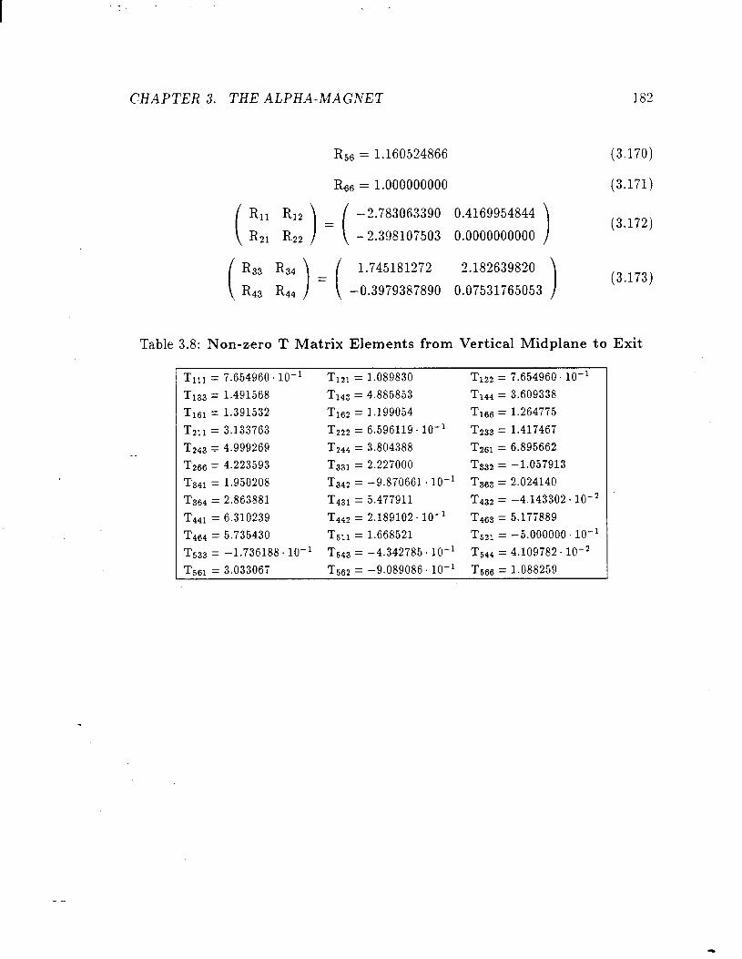
Midplane to Exit Transport
For transport, from the vertical midplane t.o the exit, tables 3.8 and 3.9 list’ non-zero
T and U mat’rix elements, respect,ively. The following are the cenkoid and R makix
elements (unlist,ed elements are zero):
c5 = 2.321049732530 (3.166)
RI6 = -2.529550131 (3.167)
Rz6 = -2.179660432 (3.168)
RS2 = -0.9089085575 (3.169)
-
CHAPTERS. THEALPHA-MAGNET 182
Rs6 = 1.160524866 (3.170)
RG6 = 1.000000000 (3.171)
-2.783063390 0.4169954844
-2.398107503 0.0000000000 (3.172)
Table 3.8: Non-zero T Matrix Elements from Vertical Midplane to Exit
Till = 7.654960.10-l Tlzl = 1.089830 Tlz2 = 7.654960.10-l
T133 = 1.491568 T143 = 4.885853 T144 = 3.609338
T161 = 1.391532 Tl62 = 1.199054 Tls6 = 1.264775
Tzll = 3.133763 T222 = 6.596119.10-’ T233 = 1.417467
T243 I 4.999269 T24.j = 3.804388 Tz61 = 6.895662
T266 = 4.223593 T331 = 2.227000 T332 = -1.057913
T341 = 1.950208 T342 = -9.870661. 10-l T363 = 2.024140
T3fj4 = 2.863881 T431 = 5.477911 T432 = -4.143302. 1o-2
T441 = 6.310239 T442 = 2.189102. 10-l T463 = 5.177889
T464 = 5.735430 T511 = 1.668521 T521 = -5.000000~10-’
T533 = -1.736188.10-l T543 = -4.342785.10-l T544 = 4.109782. 1O-2
T561 = 3.03306i T562 = -9.089086. 10-l T566 = 1.088259

CHAPTER3. THEALPHIZ-MAGNET 183
Table 3.9: Non-zero U Matrix Elements from Vertical Midplane to Exit
Ullll = -1.360 u1211 = -5.249. 10-I U12z2 = -4.872. 10-l
U1331 = 2.309
U1432 = -7.406
UlSll = -4.089
tJ1631 = 5.964. 1O-4
IT1643 = 4.234
U1662 = -7.334. lo-’
1-12221 = -1.361
U2431 = 1.181
U2442 = -2.i50
tJ2fj22 = -1.23i
Ui,=j41 = -4.345 1o-3
U26‘jl = -4.114. 10’
Ii3321 = -3.620
tJ3411 = 4.993
U3431 = 5.003. lO-4
U3444 = -2.195
tJ3fj41 = 9.078
us664 = 3.409
U4322 = -1.567
u&J21 = -2.893
U4433 = -1.323 . 10’
u4631 = -2.196 10’
U4642 = -2.630
U&64 = -1.633. 10’
U5221 = -9.179.10-l
U5332 = 2.105. 10-l
U5441 = -4.254
U5621 = -2.375
Us643 = -5.601
U5662 = -8.523 . 10-l
tJ1332 = -3.196
U1441 = 2.017
u1621 = -9.537. lo-’
tJ1633 = 1.353
IT1644 = 3.638
171,366 = -1.969
U2331 = 2.331
tJ2432 = -5.745
tJ2611 = -3.95i. 10’
r-12631 = -3.4%. 1o-3
U2643 = -1.426
UZfj66 = -1.528. lo1
IT3322 = -3.336. lo-’
U3421 = -4.032
U3433 = -4.874
tJ3631 = 5.245
IT3642 = -4.158
U4311 = -9.066
u4333 = -2.991
U4422 = -1.724
U4443 = -1.849. 10’
U&,32 = -3.155
tJ4643 = -5.769. 1o-4
IT5111 = -9.178. 10-l
U5222 = 4.545. lo-’
U5431 = -6.162
1-75442 = 4.173. lo-’
U5622 = -8.343. 10-l
Us644 = -3.846
tJ14~1 = 4.658
U1442 = -4.261
tJ1622 = 3.828. lo-’
U1641 = 6.949. 1O-4
U16fjl = -4.413
Uzlll = -1.336. 10’
U2332 = -2.750
1-12441 = -2.352
u2621 = -3.419. 1o-3
u2,j33 = 7.009. 10-l
tJ2644 = -2.138
u3311 = 3.497
U3333 = -1.167
IT3422 = -2.847 ’ lo-
U3443 = -6.236
us632 = -3.290
tJ3663 = 1.371
u4321 = -3.494
U4411 = -1.456. lo1
u4431 = -5.345.10-4
U4444 = -8.388
u4641 = -2.962. 10’
U4,j63 = -1.386. lo1
U5211 = -1.307
U5331 = -2.232
Us432 = 1.565. lo-’
U56ll = -3.337
us633 = -1.941
IJ5661 = -4.550
U5666 = -1.923
.
CHAPTER 3. THE ALPHA-hIAGNET 184
3.6 Effects of Field Errors
All of the above analysis of t.he alpha-magnet assumes that. the functional form of
the magnet.ic field is that’ of a perfect. quadrupole. In realit’y, no magnet. is ideal.
A review of the derivat,ion of the scaled equation of motion shows that. non-linear
t.erms in the magnetic field will, strictly speaking, invalidat,e the scaling. In odher
words, the magnet’ will not. be strictly achromatic, as a perfect, alpha-magnet, would
be. One result’ of this is that the nominal ideal traject,ory (i.e., the trajectory injectSed
at’ incidence angle 8,) will no longer exit, the magnet at, the same location t.hat it’
ent,ered at,.
Magnet,ic field errors are a fact of life in accelerat,or physics. The favored approach
t.o dealing wit.h them is to evaluate the effect’ of specific t,ypes of errors (e.g., higher-
order mult,ipoles) with an eye t.oward what, level of error one’s application can tolerat,e.
In accordance with this, I have studied the effect of cert,ain t’ypes of field errors: such
as sextupole berms, to find what, effect they have on the performance of the alpha-
magnet. (Similar, less complet,e work on this problem is report,ed in 1321.) It has
been found from computer st.udies that. for a variet.y of errors, the residual dispersion
aft,er t,he alpha magnet, can be reduced t,o acceptable levels by modifying the injection
angle, 8i, in such a way as to cause the ideal trajectory t,o once again exit. at’ t’he
ent,rance point. If the magnet, retains reflect,ion symmet,ry about, the plane q2 = 0,
it. is always possible to find such a value of Bi, which I will call t9,, or t,he “mirror
angle”. The reader can convince himself of t,his by reviewing t,he argument. by which
I proved that’ the perfect, alpha-magnet’ has such an inject,ion angle, namely 8,.
The field in the imperfect’ alpha-magnet can be expressed as
B(s) = g(qs,O, ql) + AB(q)
(Q3AQ,> + AB(z); (3.174)
where .AB(q) is t,he depart,ure of the field from a true, uniform quadrupole field and,
as before, Q = qa.
Comparison with equation (3.83) shows thatS the scaled equation of mot.ion wit,h
CHAPTER3. THEALPHA-MAGNET 185
field errors is
Q” = - &Q’ x B($);
= -1Q’ x 1+6
(Qso, Ql) + A+}
(3.175)
(3.176)
3.6.1 Multipole Errors
Wit,h this equation in hand, it. is possible t,o evaluate the effect. of various field errors.
Not,e that’ since Q appears only as a multiplicat.ive fact.or for the field error, it’ is
still possible to find result,s with some universalit’y. In particular, if AB is a pure
multipole error, t.hen the effect of the field error in the equation of motion will have
a well-defined scaling with Q and the mult,ipole coefficient.
Multipole fields can be classified as upright’ or rotated[6], depending on whether
the magnetic-fields are changed in sign upon reflection of the magnet through the
qs = 0 plane or not, respectively. Upright multipoles have field lines that cross the
qs = 0 plane with normal incidence. For rotat,ed multipoles, field lines do not, cross
the qa = 0 plane. Clearly the alpha-magnet. has upright’ symmetry, and if one confines
oneself to errors bhat, do not alt,er t#his symmetry, then one can express errors in the
alpha-magnet, in t#erms of the upright. multipoles. For example, any deviation of the
poles from a hyperbola will produce only upright multipole errors, as will displacement.
of t.he mirror plane, since neit,her of these errors changes t,he fact’ that, the field lines
cross qs = 0 with normal incidence.
The field due t,o a pure upright’ mult.ipole is[6] :
1nPi n-2m
AB, = A, C ( -Qm-i q1 s3”-’ &
Ill=1 (n - 2m)! (2m - l)! (3.177)
l(n+l)/2J n-2m+l 2m-2
+An c m=l
(-‘)“-‘(n 4’2, + I>! (22 _ 2)!q3r
where n _> 1 is an int.eger, the “order” of the multipole. n = 1 is a dipole, n = 2 a
quadrupole, and so fort,h.
For insert,ion into equation (3.176)) this must, be rewritten in terms of scaled

CHAPTER 3. THE ALPHA-MAGNET
coordinat,es, as
QAB, g
= l+J QF2" Q;"-' ..
Mn m~l(ml'm-l (n - 2m)! (2m - I)! Q1 l(n+l)DJ +M, 1 (-l)m-1 Qi'-2m+1 Q,G"-" g3,
m=l (n - 2m + l)! (2m - 2)!
where I have defined the dimensionless normalized mult.ipole st.rength
M,G% gQn-2
186
(3.178)
(3.179)
Even without, int,egrat,ion one can conclude that for t.he same fractional multipole
error, $, the perturbation is stronger for smaller Q, i.e., for alpha-magnets operat,ed
so as t,o obt#ain larger values of 41. This is as expect.ed, since the multipole field grows
as qf. As expect.ed, in the limit’ of very large Q, i.e., very small ql, multipole errors
have no effect..
It, is of course possible t>o compute the matrices for equation (3.176) with AB as
given by (3.179) as was done for t#he equat.ion of motion without’ field errors. The
mat.rices thus obtained are to be considered funct.ions of M,, with M, ultimabely
a funct,ion of Q. Hence, if t,he matsrices are found for some particular value of M,
for some particular n, t,hen if t,he matrices are scaled to some particular value of Q
according to equation (3.93), t.he result, is appropriate to a multipole strengt.h of
A, = M,~cC-‘-~. (3.180)
I have writt,en a computer program, serrors, which computes third-order scaled
alpha-magnet. matrices in the presence of various types of field errors, including mul-
tipole errors. Figures 3.10 through 3.12 show the effect, of sextupole errors on the
mirror-angle (8,), Ql, and the non-zero elements of the matrix R. Not,e t,he particu-
.larly strong effect. in the vertical plane.
3.6.2 Entrance-Hole-Induced Errors
I performed magnetic measurements on t’he SSRL alpha-magnet. to assess the devi-
at,ion of the field from an ideal quadrupolar field. Figure 3.13 shows the measured
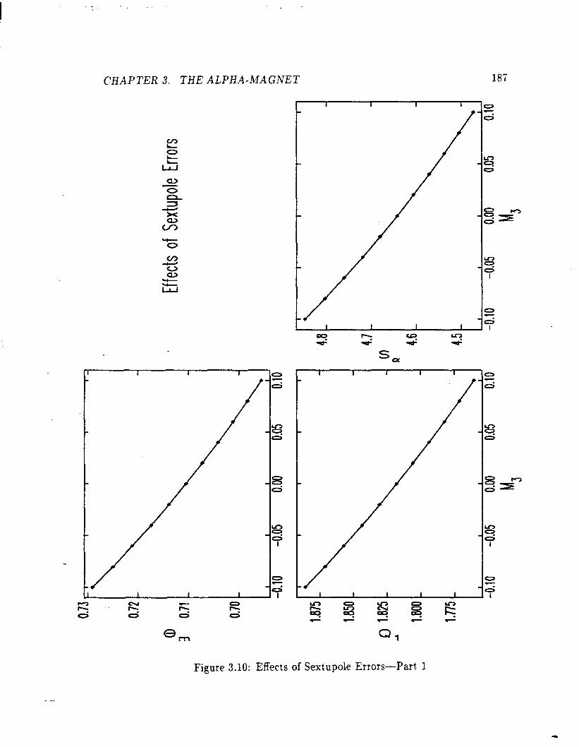
CHAPTERS. THEALPHA-MAGNET
ir d
Qm
E . g g - - - Ql
Figure 3.10: Effects of Sexdupole Errors-Part, 1

CHAPTER 3. THE ALPHA-MAGNET
I I I I I I
Figure 3.11: Effecb of Sexhpole Errors-Part 2
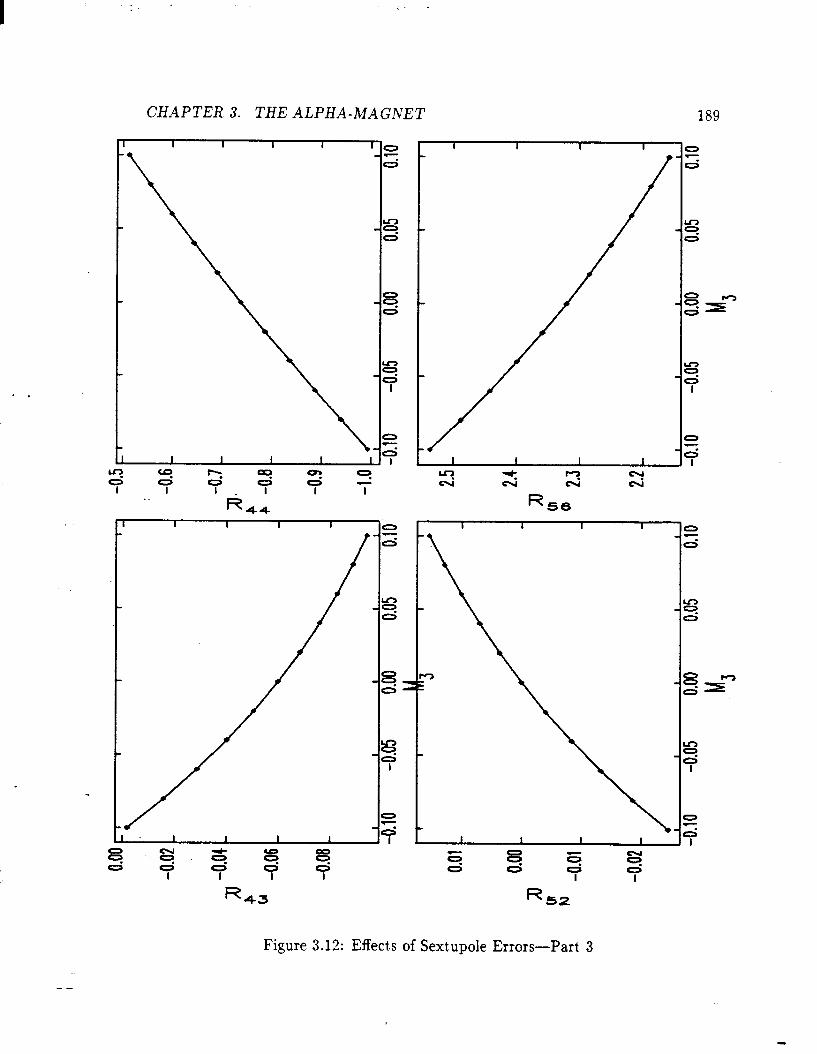
.
CH.4PTER3. THEALPHA-MAGNET
9 LD Y -1 . .
e44
I I I I lo
Figure 3.12: Effects of Sext.upole Errors-Part 3
--
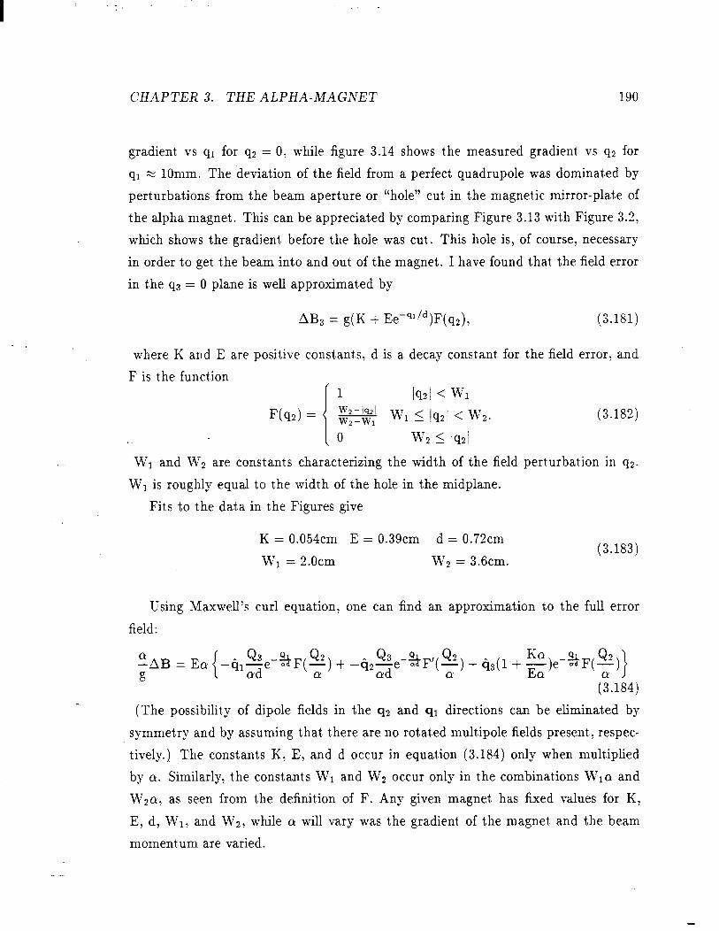
I :
CHAPTER 3. THE ALPHA-MAGNET 190
gradient. vs q1 for q2 = 0, while figure 3.14 shows t,he measured gradient, vs q2 for
91 z 10mm. The deviation of the field from a perfect quadrupole was dominat,ed by
perturbat,ions from t,he beam apert,ure or “hole” cut. in t,he magnet.ic mirror-plat,e of
the alpha magnet. This can be appreciat,ed by comparing Figure 3.13 with Figure 3.2,
which shows the gradient. before the hole was cut. This hole is, of course, necessary
in order t,o get, t’he beam into and out of the magnet. I have found that, the field error
in t,he qa = 0 plane is well approximat,ed by
4Bg = g(K + Eemqlid)F(q2), (3.181)
where K and E are positive constants, d is a decay const.ant. for the field error, and
F is the function
I
1 Is21 < Wl
F(qd = ?i2-/921 WI 5 /q2/ < W2. b2-W1
(3.182)
. . 0 w2 L Is21
Wi and W2 are constants charact.erizing the width of the field pert,urbat.ion in q2.
Wi is roughly equal to the widt’h of t,he hole in the midplane.
Fits to the dat,a in t,he Figures give
K = 0.054cm E = 0.39cm d = 0.72cm
Wi = 2.0cm Wp = 3.6cm. (3.183)
Using Maxwell’s curl equation, one can find an approximation to the full error
field:
Q3 -a Q2 -Qi;L;ie adF(T) + -G2Ze
Q2 Q3 -sF’( ;) + G3( 1 +
(The possibility of dipole fields in the q2 and ql directions can be eliminated by
symmetry and by assuming that. there are no rotated multipole fields present, respec-
tively.) The const,ants K, E, and d occur in equation (3.184) only when multiplied
by a. Similarly, t’he constant,s Wi and W2 occur only in the combinat,ions Wio and
W2a, as seen from t,he definit,ion of F. Any given magnet has fixed values for K,
E, d, Wi: and W2, while a will vary was t.he gradient, of the magnet and the beam
moment,um are varied.

-
CHAPTER3. THEALPHA-MAGNET
-
II
191
VB (At-b. Units)
Figure 3.13: Hole-Induced Gradient. Errors vs q1

-
CHAPTER3. THEALPHA-MAGNET
. . !G i
l
I I I I I I I I 1
192
In E;
I
76 (Arb.lJnits)
Figure 3.14: Hole-Induced Gradient Errors vs q2
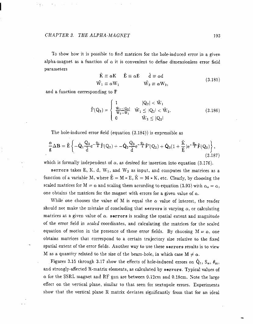
CHd4PTER3. THEALPHA-MAGNET 193
To show how it. is possible to find matrices for the hole-induced error in a given
alpha-magnet, as a function of CY it is convenient t.o define dimensionless error field
paramet,ers
l? E aK fi E oE d s ad
w, E awl I@2 E QW2, (3.185)
and a function corresponding to F
1 IQ21 < *I
p(Q2) = - $& 5 IQ21 < m2. wz-w1
0 \?i’2 5 IQ21
(3.186)
The hole-induced error field (equation (3.184)) is expressible as
:4B=E i-
-blQ3 -$- y d F(Q2) + -Q2 ;1 ^ se-%@‘(Q2) + &(l + $e-%$jQ,) , 1
. . (3.187)
which is formally independent’ of a, as desired for insertion into equation (3.176).
serrors takes E, K, d, WI, and W2 as input,, and computes the mat,rices as a
funcdion of a variable M, where E = M * E, K = M * K, et,c. Clearly, by choosing the
scaled mat.rices for M = Q and scaling them according to equat,ion (3.93) wit.h Q, = o,
one obtains the matrices for the magnet, with errors for a given value of a.
While one chooses the value of M is equal t,he o value of interest, the reader
should not, make the mistake of concluding that. serrors is varying Q, or calculating
mat’rices at’ a given value of c~. serrors is scaling the spatial extent, and magnit’ude
of the error field in scaled coordinates, and calculat,ing the matrices for the scaled
equation of motion in the presence of t.hese error fields. By choosing M = a, one
obt.ains mat.rices that correspond to a certain traject*ory size relative to the fixed
spat.ial ext,ent, of the error fields. Another way to use t.hese serrors results is to view
M as a quant,it.y related to the size of the beam-hole, in which case M # Q.
Figures 3.15 through 3.17 show the effects of hole-induced errors on Qr, S,, 8,,
and strongly-affected R-matrix elements, as calculated by serrors. Typical values of
CY for the SSRL magnet and RF gun are between 0.12cm and 0.18cm. Not.e t,he large
effect on the vertical plane, similar to t,hat seen for sextupole errors. Experiments
show that the vert,ical plane R matrix deviat.es significant,ly from that for an ideal

CHa4PTER3. THEALPHA-MAGNET 194
magnet, a subject, to which I will ret,urn in the next section. Running experience
shows t.hat. injection angle corrections of lo-20 mrad are needed, with the sign such
as to make 8 smaller. It’ is unclear, however, what. part, of this is due to field errors
and what. part is required by alignment, errors. The real value of these calculations is
to evaluat,e the magnit.ude of the effects of such errors, t,o see whet,her the injection
angle correction required for realistic error levels is feasible or not.

CHAPTER 3. THE ALPHA-MAGNET
Q> 5 - * -
N 0
=G 09
Ql
-
Figure 3.15: Effects of Hole-Induced Gradient. Errors-Part, 1
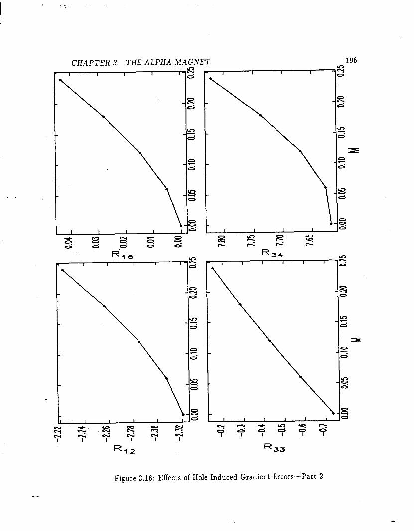
CHAPTER 3. THE ALPHA-MAGNET
-3 d
u7
d
0 - d
-s d
R 34
Figure 3.16: Effects of Hole-Induced Gradient, Errors-Part. 2
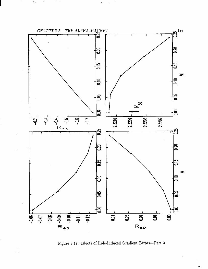
-
CHAPTER 3. THE ALPHA-hfAGNET L ,
-2% c d
d
0
R 43
Figure 3.17: Effects of Hole-Induced Gradient, Errors-Part’ 3
CHAPTER3. THEALPHA-MAGNET 198
3.7 Alpha-Magnet Beam-Optics Experiments
A commonly-made measurement’ on beam-transport systems is that of det,ermining
t,he t,ransverse cent.roid offset, of the beam downstream from a st,eering magnet, as a
function of t,he angular kick impart*ed by that st,eering magnet. The linear derm of
a fits to the offset. vs kick angle gives the ri2 (or ra4 for a vertically steering magnet)
matrix element, for transport, from the steering magnet, to the place where the cent.roid
position is measured.
The Gun-to-Linac transport, line (see Chapt,er 5) has horizontal and vertical s-
teering just before t,he alpha-magnet, and a phosphorescent’ screen downstream of the
alpha-magnet, (t,he “chopper-screen”, since it, is part. of the chopper tank). There is
also a phosphorescent, screen inside the alpha-magnet, (the “alpha-magnet, screen”)
that, intercepbs the beam when the alpha,-magnet, is t,urned off. These phosphorescent,
screens are-viewed via closed-circuit, TV. In addition, a Lecroy 9450 digit.al oscillo- . . scope is available t,o digitize t,he TV scan, permit.ting accurate measurement’ of both
horizont,al and vertical beam positions. All that’ is required is. t,o calibrat,e t,he TV
sweep using features on the screens for which the positions are known (e.g., the edges
of the screen).
I will let Li denote t.he dist.ance from the cent,er of t,his steering magnet, known as
GTL-CORR2, to the “crossing-point,” of the alpha-magnet (qi = q2 = qs = 0). Also,
L2 and La denot,e, respecdively the distance from the crossing-point, to the alpha-
magnet. screen, and from the crossing-point t,o t’he screen aAer t.he alpha-magnet.
L1 is found to be 117 mm, and La to be 459 mm, where I use values from updat,ed
engineering drawings, checked by my own measurements wit,h a ruler. The distance
from the crossing-point to t,he screen in t,he alpha-magnet, 200 i lOmm, with the large
uncertaint’y being due to the way the screen is held inside the alpha-magnet on long,
easily-bent, copper tubes.
3.7.1 Characterization of the Steering Magnet
I performed magnetic measurement,s on GTL-CORR2 with a quadrupole and a.n
alpha-magnet-simulating iron plat,e in the proper positions relative to GTL-CORR2.
The magnetic field as a function of longitudinal posit.ion z is shown in figure 3.18,

. -
CHAPTER3. THEALPHA-MAGNET
Figure 3.18: Magnetic Measurements for GTL,CORR:!
199

CHAPTER3. THEALPHA-MAGNET 200
and indicades t,hat, the equivalent. angular kick for a zero-length steering magnet, is
18mm ahead of the geometric cent,er of the magnet (which coincides with the peak
of the magnetic field vs z). Hence, GTL-CORR2 can be simuladed by a zero-length
s6eering magnet. that is Li + 18mm from the alpha-magnet, crossing point. I wiIl thus
let. L1 + Li + 18mm, and treat, GTL-CORR2 as a zero-length deflector.
Because GTL-CORR2 is in close pr0ximit.y to both the alpha-magnet and the
immediat,ely preceding quadrupole, it, is advisable to check t,hat, the calibration of an-
gular deflect,ion vs driving current. (obtained from magnetic measurements) is correct.
This was done using the alpha-magnet screen, since the transport, to this screen from
GTL-CORR2 is described by a simple driftspace matrix:
(3.188)
In t.his sect,ion, I will use r(‘) t,o represent, t,he r-matrix from GTL-CORR2 to point i,
where i is 1, 2, or 3 for the crossing-point, alpha-magnet’ screen, or chopper-screen,
respectively. I leave off the dispersive and pat,h length elements t.o shortmen t,he not.a-
t,ion.
This check was carried out. using the magnetic measurement,s to set GTL-CORR2
to a series of nominal horizontal (or vertical) deflection angles, Bnom,i, and measuring
t,he resulting horizontal (or vertical) displacement, xi, at. the chopper screen. A linear
fit, t0 Xi VS onom,i gives the nominal value of rem), uncorrect,ed for errors in the
deflection angle. Since it. is that, ri2 (2) = rE’ = 0.337 & O.OlOmm/mrad (this is just.
LI + L2) the acfual angular deflection is readily calculated, giving
@act = @nom rem)( mm)
0.337 or O.OlOmm/mrad (3.189)
Linear least-squares fits t,o t,he dat,a from these experiments gave Tern) = 0.3055
O.O06mm/mrad and rgrn) = 0.3221 O.O15mm/mrad, from which I conclude t,hat’
8 - 8,,,,,0.91 i .03, x,act - (3.190)

CHAPTERS. THEALPHA-MAGNET 201
and
8 y,act - - 8y,rmmO.96 5 .05. (3.191)
3.7.2 Comparison of Experimental Results and Theory
Having corrected the calibration of GTL,CORR2, I then did a series of measurements
of r$) and rg’ for various alpha-magnet, gradients for const,and beam momentum. For
these experiments, t.he low-energy scraper inside the alpha-magnet was set’ bo allow
only about &5% moment.um spread t,hrough, t,o lessen any possible ambiguit.y about
what. t*he momentum of the particles seen on the chopper screen was. Spectrum
measurements allow the det,ermination of the median momentum of the particles let
through, and this quantity was used as the effective moment,um of the beam centroid.
Table 3.10 summarizes t.he results.
In order to compare these results to theory, it is necessary to use serrors-
calculated scaled mat’rices for the appropriate values of the error parameter M (i.e.,
M = cy, for hole-induced errors), t’o scale these matrices to the values of Q listed in
the t,able, and to finally concat,enat,e these matrices with drift space matrices:
r = d( Ls)A-I( a)R( M)A( cr)d(Li), (3.192)
where d(L) represents the matrix for a drift, space of length L. Table 3.11 gives the
results of this procedure, listing the r 12 and rs4 values corresponding to each of the
cases in Table 3.10. Also listed for comparison are the values for a perfect. alpha-
magnet. These results are displayed in figures 3.19 and 3.20.
As seen from Figure 3.20, the rg” s are very sensitive to errors, hence the agree-
ment, seen here may be fort,uitous. In the same vein, some disagreement is hardly
unexpect’ed.
With the exception of the anomalous point at cr = 0.166, all of the measured
ri2’s are 5-10% smaller than the theoret,ical values for the alpha-magnet. with errors.
The first, explanation of the discrepancies in the horizont,al plane one might entertain
is t,hat, the moment,um (or, equivalently, the alpha-magnet gradient, calibration) is
in error by 5-10%. This, however, would not. explain the discrepancies observed.

.
CHAPTER3. THEALPHA-MAGNET 202
First, the correction of the calibrat,ion of GTL-CORR2 would eIiminat,e any effects of
moment,um errors on deflecdion angle. Hence, any momentum errors would come int,o
play only through the alpha-magnet. However, as seen from the slope of r12 vs o for
the t,heoretical dat.a in Figure 3.19, a very large moment.um error would be required to
explain the observed discrepancy. For t.he point, with a = .121, for example, one would
need to postulat,e a moment,um error of about, a factor of two, which I do not consider
remot,ely possible. A remaining possibiIit,y is t,hat, the calibration of GTL-CORR2 is
in error, due to inaccurate knowledge of the position of the alpha-magnet, screen. A
5-10% error in this calibration would require a. 15-30mm error in the position of t,he
screen. This is not’ inconceivable, given the lack of precision in the screen assembly.
Table 3.10: Alpha Magnet rr2 and rs4 Measurements
gradient. <P> OL (3) r12
(3) r34
. . (G/c4 MeV/c l/cm mm/mrad mmfmrad
255.1 & 1.3 3.00 & 0.04 0.160 i 0.001 -0.743 i 0.014 0.006 i 0.005 202.9 i 1.0 2.71 i 0.04 0.150 & 0.001 -0.672 i 0.012 0.070 i 0.002
172.8 i 0.9 2.83 i 0.04 0.135 & 0.001 -0.716 i 0.012 0.120 zt 0.004
149.1 i 0.7 2.81 i 0.04 0.126 i 0.001 -0.730 i 0.016 0.149 i 0.004
129.9 i 0.6 2.80 i 0.04 0.118 i 0.001 -0.739 i 0.018 0.180 i 0.005
Table 3.11: Calculated Alpha-Magnet r12 and ~4
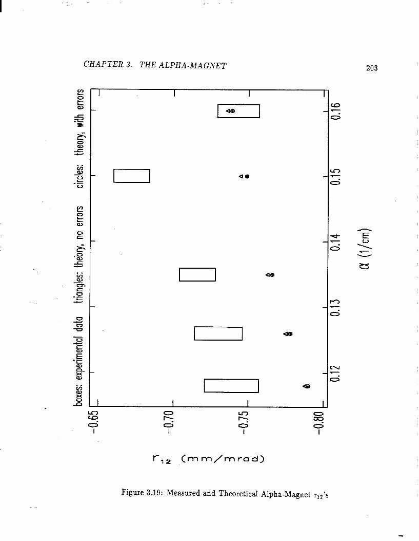
A 3
3 \
3 ii
a
V
boxe
s: ex
peri
men
tal data tri
angl
es:
thek
q, no
er
rors
ci
rcle
s: th
eory
, w
ith e
rror
s
-0
65
.
-0
70
6
-0
75
.
-0
80
.
s 8 0
0.12
0.
13
0.14
,
015
016 .
Q (l/
cm)
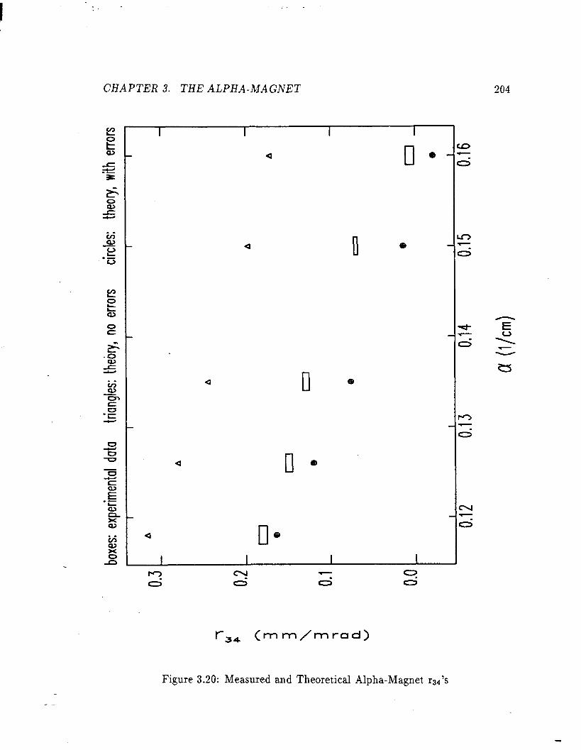
CHAPTER3. THEALPHA-MAGNET 204
. . z u .L v
!z t Q)
a
a
a
a
a
II
0
e
13 8
II 8
0
r 34
(mm/mrad)
Q -T
C
u -T
C
. -.
C
P -.
c
C -.
c
0
5
D - 5
c, - 3
N
5
Figure 3.20: Measured and Theoretical Alpha-Magnet. rs4’s

.
Chapter 4
Longitudinal Dynamics
In Chapt,er 2, I described the longit.udinal phase-space dist,ribut,ion of the RF gun
beam, and indicat.ed that this phase-space ill-suits the beam to direct’ injection into
.a S-Band linear accelerator section (here-aft,er referred t,o simply as “the linac”). In
this chapter, I will show why this is so, and how the gun longitudinal phase-space may
be t,ransformed int.o somet.hing that, is amenable to further acceleration. At, issue is
the need for a small fractional energy spread, which is required for efficient, transport,
through a subsequent, beamline, use as the drive for FELs, and other applications. I
shall also show how the rather long (25 ps or so) bunch at t,he end of the gun can-at,
least in t,he absence of excessive errors and space-charge effects-be compressed to
a very short, 1-2 ps bunch, t.hus promising bhe pot,ential of very high peak currents,
somet,hing that. is desirable in FEL applications, among ot.hers.
Discussion of t,he t,ransformation of t,he gun longit,udinal phase-space cannot, take
place without, an understanding of the longitudinal dynamics of electrons in magnetic
syst,ems and linear accelerators. I will first, discuss longit,udinal dynamics in linear
accelerat,ors, and in particular how one can predict, the longitudinal phase-space at’
the end of a finit,e-length accelerat,or when start.ing with a beam that, is not. fully
relativistic. This discussion will show why the RF gun beam is unsuit.ed to direct
injection int.o the linac.
I will t#hen discuss how magnetic beamline elements can be used t.o alter a beam’s
longit,udinal phase-space. Using results from Chapter 3, I will dem0nstrat.e that. an
alpha-magnet, has advantages in such an application. I will present. the resu1t.s of 205

.
CHAPTER 4. LONGITUDINAL DYNAMICS 206
optimized alpha-magnet-based bunch compression, with inclusion of detailed longi-
dudinal dynamics calculahions, and show how t.his achieves significantly bett.er resu1t.s
compared to t,he first,-order method of simply inject,ing t,he short.est, possible bunch
into the linac.
Finally, I will present, results that include consideration of aberrations in the gun-
to-linac transport. line, and use t.hese results to compare the SSRL preinjector to other
projects.

CHAPTER 4. LONGITUDINAL DYNAMICS 207
4.1 Longitudinal Dynamics in Linear Accelera-
tors
There is extensive literat,ure on longitudinal dynamics in linear accelerators[56, 55,
41, 691. Rather than att,empting to duplicat’e that work here, I shall simply make
use of some of the results. In particular, I shall use the commonly-made assumption
[41, 551 that. the longitudinal elect.ric field of a t’raveling-wave linear accelerat,or may
be approximat,ed by the first space-harmonic,
E,(z, tm) = E - cos(kz - wt), 0 5 z < L, (4.1)
where k is the propaga.tion constant,, w/(2~) is the RF frequency, L is t,he length
of the st#ruct.ure (which starts at z=O), and E is a constant.. For a velocit.y-of-light,
st.ruct,ure such as t.he SLAC constant-gradient’ structure used for the SSRL linac,
w = kc, c being the speed of light. While the actual field contains components with
propagation constants k, = k + T, where n is an integer and p is the periodic length
of t,he structure[56], these components have phase-velocities w/k, less than the speed
of light: and hence a relativistic particle will not remain in phase with any but t.he first.
space-harmonic. Because of t.his, the higher space-harmonics impart no net, energy
to a relat,ivist,ic beam. Traveling wave accelerat,ors are specifically designed to have
small amplit,udes in t.he non-synchronous space-harmonics, since these carry away RF
power without. cont.ribut*ing to acceleration[56].
The equations of motion for an electron in the presence of dhis field are found
from the Lorentz force. For 0 I z 2 L,
dp -*cos(kz - w(t, - t,) + &)
dt = m,c dz
dt.=
(4.2)
(4.3)
where p G fir is t,he momentum and & is the initial RF phase for the fiducial particle,
which enders the accelerat,or at. t. = t,. I will assume that, -eE > 0, so t.hat, the fiducial
particle is accelerat,ed for &, = 0. If 40 < 0, t,hen t,he fiducial particle is “behind the
crest,“, meaning t.hat. if it, is sufficiently non-relativistic, it, ma,y fall furt.her behind; if
it, falls back far enough (or if &, < ~/2) the particle will be decelerated. Similarly,

-
CHAPTER 4. LONGITUDINAL DYRAMICS 208
if $,, > 0: the fiducial particle is “ahead of the crest.“, meaning that, if it’ is not. fully
relativistic, it, may fall back to be nearer t,he maximum accelerat,ing phase.
4.1.1 Approximate Treatment for Highly-Relativistic Par-
t icles
In general, these equations are unsolvable by analytic means, being coupled and non-
linear. However, for p2 >> 1, the electrons are fully relat,ivistic, and z = c(t# - ti),
where ti is the time at, which t.he particle ent,ers the accelerator. In this case, t,he
acceleration experienced by any part.icle is const.ant:
dp -eECOS(-Ld(ti - to) + 40).
db = m,c
The solution, for t; 5 t. 5 ti + L/C,
. . p(t,) = p(ti) - (t - ti)- eE COS(-Ld(tmi - to) + $0)~
n-w
may be used to determine the final moment,um after an accelerat,ing section of length
L:
eEL COS(-Ld(t,i - to) + $o), Pf = Pi - - m,c2
(4.6)
where pi = p(ti) and pf = p(t.f).
Since the “useful” elect.rons out. of the RF gun typically have p > 4, giving ,i? 1 0.9i,
this result, is of more t,han academic int,erest,. Though it is far from exact, it. is a useful
approximat.ion, and aids t,he underst,anding of t.he detailed result,s.
The quant,it’y $i = -ti(ti - to) + &, is t.he initial phase for some particular particle,
even if t.he particle is non-relativistic. However, for a particle that is init.ially fully
relativist,ic, t,he inibial phase is also the RF phase throughout, the accelerat’or section.
Hence, if it. is desired t,o accelerate a bunch of relat,ivistic particles wit,h small final
momendum spread, it, is necessary to inject’ these particles int,o the accelerat,or over a
sufficient#ly small time-int,erval. Suppose t,hat. the bunch initially has no moment8um
spread, and that’ & = 0 to obtain maximum acceleration of t.he fiducial part,icle.
Assume further t,hat, t.he fiducial particle is at, the cent,er of t.he bunch, which has
length bt. Then t.he spread in final moment,a will be
6p = (pf - pi)( 1 - COS(U6t~/2)), (43

CHAPTER 4. LONGITUDINAL DYNAMICS 209
where pf = pi - 3 is the final momentum of t’he fiducial part,icle. For wSb < 1:
t.his implies a fractional moment,um spread of
EP Pf - Pi S42 -=-- Pf pf 8’
(4.8)
where S$ = w6t is the phase spread of the incoming beam. If the beam is accelerated
to very high momentum relative to pi, then this becomes
fip S@ -=- Pf 8’
(4.9)
and one sees t,hat. the final fractional moment,um spread is, t,o first order, quadrat.ic
in the initial phase spread if one injects the fiducial (and central) part.icle at, the
crest. Hence, in order to obtain a small final momemum spread, one must inject, a
sufficienbly short bunch int,o t.he accelerator:
(4.10)
For t,he SSRL Injector, a fractional moment.um spread of less t,han 0.5% was
needed, to accommodat*e the accept,ance of the synchrotron[26]. Hence, from this
analysis one would conclude that, an initial tot.al phase-spread of less than about 12”
is required, if one ignores the initial moment,um spread in t,he RF gun beam. I shall
show below t.hat,, however, t,hat one cannot, ignore the initial momentum spread: if
one really desires such low final momentum spread. 1L’ot.e that injection with the
central parMe off the crest, will only increase the final moment,um spread for a beam
with no initial moment,um spread, while for a beam t,hat, has some initial, time-
correlat,ed momentaurn spread, inject,ion off t.he crest can be used to c0mpensat.e the
initial moment,um spread, as will be seen below.
4.1.2 Numerical Solution and the Contour Approach
Comput,er met’hods can easily solve equations (4.2) and (4.3) t,o high precision, so
it, is not necessary t*o att,empt, to find a solution t,hat. is valid for non-relativistic
eleckons. For the current, project in part,icular, t,he input, longit,udinal phase-space
--

I -,. .
CHAPTER 4. LONGITUDINAL DIWAMICS 210
dist,ribut.ion is it,self not amenable to analytical treat’ment, but. is rat.her obtained from
numerical simulations. Hence, I will move on to discuss computer-aided t.reatment, of
this problem.
For some of my computer studies, I employed another pair of equations[41], which
are useful if longit,udinal motion is one’s only interest. Rather than start. with t&he
Lorentz equat,ion, one start.s wit,h[31]
dm,c2Y
dt’ = -eve E, (4.11)
and assumes t,he velocit’y bo be parallel bo elecdric field. One form of t,he result,ant,
equations is (reference [41] gives t,hese equat,ions and a detailed discussion of t’hem)
dy dC
= E cos 2T(C - r)
. . dr 1
;i3 = 3’
(4.12)
(4.13)
whereC=f,X=%,Z=-3,andr=$$. The,RF phase for any part.icle at, z=O is
particle is 4 = -2nr, which is consist,ent with the convention I used above. In terms
of normalized elect,ric-field &, the change in y in a section of length L for an inidially
relativist,ic part.icle is
Ay = cYA< = f; (4.14)
There is no particular a,dvant,age to these equations over a similarly-scaled form
of equations (4.2) and (4.3) for numerical work -1 state t.hem because I happened
t,o use them in some of my computations. Specifically, I have writt,en a computer
program (linac-cg, where “CG” st.ands for “constant-gradient”‘) that int.egrat.es e-
quat.ions (4.12) and (4.13) for a set, of particles distribut,ed on a grid over some region
of initial (4, p) space. The program comput,es the final momentmum and phase for each
part’icle, and displays the results in contour-plot, form. From these, one can deduce
the result.ant, moment,um spread and phase spread for any particular injected bunch
simply by finding which contours are int,ersect’ed when t,he phase-space distribution
for t,he inject.ed bunch is overlayed on the cont.our graphs. Note t.hat a different plot,
must be generateed for each value of E. For the SLAC-t,ype constant’-gradient, sections

-
CHAPTER 4. LONGITUDINAL DYN+MICS 211
used for the SSRL pre-injector[70], t.he nominal energy gain per section is given by[6]
Ay = 20.4@-@iij, (4.15)
where P is t,he RF power t,o the section. Combining this with the previous equation,
using L = 3.048m and X = O.l05m, I obtain
& = 0.703JP~. (4.16)
While nominal RF power per section for the SSRL Pre-injector Linac is 30 MW,
t,he RF power to t,he first. section is limited operat.ionally to 20 to 25 MW. Since the
energy gain scales only as t.he square-root, of the momentum, bhe differences among
these are relat,ively minor. For t,his reason, and for brevity, I present. only the results
for 20 MW RF power, and display these in Figures 4.1 and 4.2.
The horizontal axis for these graphs is the phase, &, at. which the particle is in-
jected, while the vertical axis is the initial momentum, pi. As before, 4i > 0 indicat.es
injection ahead of the RF crest. The contours show lines in (4i, pi) space of con-
stant, final moment.um, pf, or final phase, &. The momentum cont,ours are spaced
by Apf = 4.2 and the phase cont’ours by A& = 10”. The labels for t.he contours are
posit,ioned so that. the cont,our closest, t*o the lower left. corner of the first letter in the
label is the one to which the label applies.
A bunch wit,h an initial longitudinal phase-space distribution that, mat,ches a con-
stant. final momentum cont,our will be accelerat,ed t.o zero momentum spread, and
similarly for a bunch that mat,ches a constant’ final phase contour. Regions where
many lines occur in a small area indicat,e rapidly changing final paramet,ers as a func-
tion of init.ial parameters. Regions where the contour lines are widely spaced indicat.e
slowly changing final parameters as a function of init.ial parameters.
Examination of Figure 4.1 shows that,, as expected from the above analysis, the
final-moment*um cont,ours are most widely spaced for $i near zero. The region of
widest, cont,our spacing moves to posit,ive 4; as the initial momentsum decreases be-
cause, for a bunch of non-relativistic electrons, injection at slight,ly positive #i result,s
in the bunch center falling back toward c$ = 0 as the electrons gain energy. If such
a bunch were inject,ed at di = 0, it, would fall back to & < 0 before reaching rela-
tivistic velocities, and as a result, the bunch momentsum would be decreased while its
moment’um spread would increase.

.
CHAPTER 4. LONGITUDINAL DYNAMICS 212
iI2 -
s -
s
- z
OZ
4-
0
I
0 m 00 t- CD -
Figure 4.1: Constant Final Momentum Cont,ours

CHAPTER 4. LONGITUDINAL DYNAMICS
r
- I -
213
Figure 4.2: Constant Final Phase Cont,ours
--
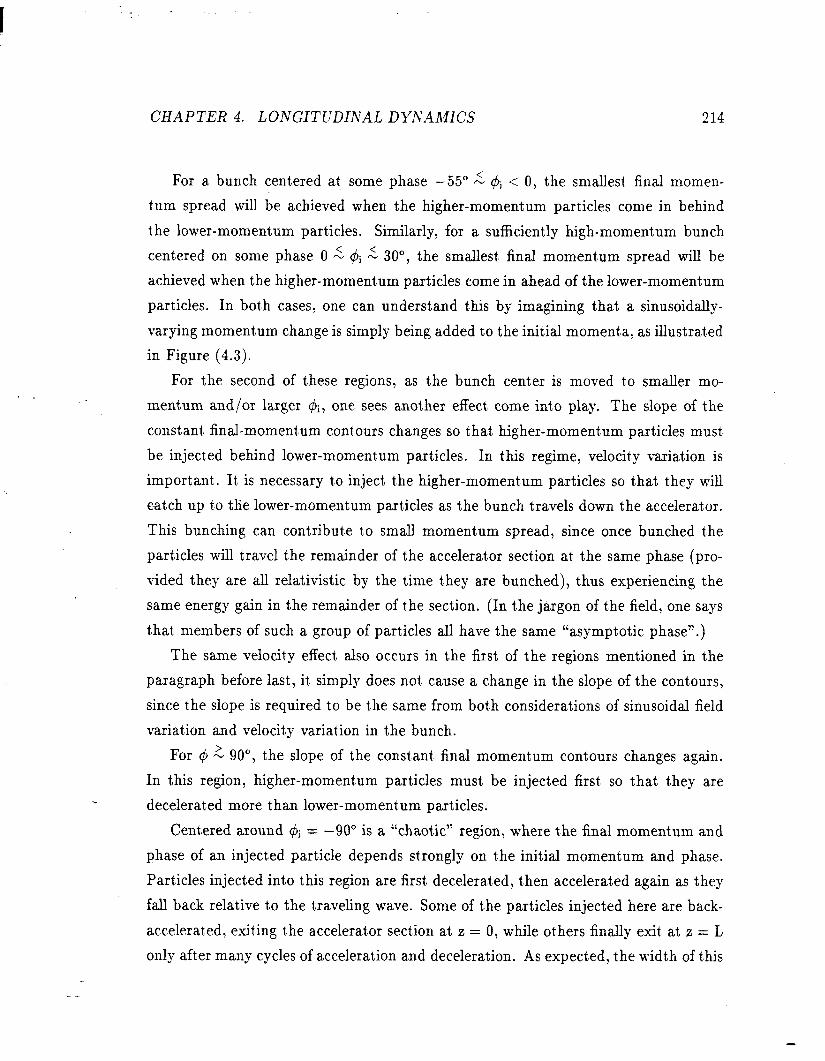
-
CHAPTER 4. LONGITUDINAL Dl’hTAhUCS 214
For a bunch cent.ered at’ some phase -55” A & < 0, the smallest final momen-
t,um spread will be achieved when t.he higher-momentum particles come in behind
the lower-momentum particles. Similarly, for a sufficiently high-moment’um bunch
centered on some phase 0 5 4; 2 30”, the smallest. final momentum spread will be
achieved when the higher-moment.um particles come in ahead of the lower-moment,um
particles. In both cases, one can understand this by imagining that a sinusoidally-
varying moment,um change is simply being added to the initial momenta, as illustrat,ed
in Figure (4.3).
. , For the second of these regions, as the bunch cent.er is moved to smaller mo-
ment.um and/or larger di, one sees anot,her effect come int.o play. The slope of the
constant, final-momentum cont,ours changes so that, higher-momentum particles must
be injectsed behind lower-momentum particles. In this regime, ve1ocit.y variation is
important. It’ is necessary to inject the higher-momentum particles so that. they will
c-at.ch up t,o the lower-momentum part,icles as the bunch travels down the accelerabor.
This bunching can contribute to small momentum spread, since once bunched the
particles will t,ravel the remainder of the accelerator section at, 6he same phase (pro-
vided they are all relativistic by the time they are bunched), thus experiencing the
same energy gain in the remainder of the section. (In the jargon of the field, one sa.ys
that’ members of such a group of particles all have t,he same “asymptotic phase”.)
The same velocit’y effect also occurs in the first of the regions ment,ioned in t,he
paragraph before last, it, simply does not. cause a change in the slope of the cont,ours,
since the slope is required to be t.he same from both considerations of sinusoidal field
variation and velocit’y variat,ion in the bunch.
For 4 2 90”, the slope of the constant, final momentum contours changes again.
In this region, higher-momentum particles must, be inject,ed first, so that they are
decelerated more than lower-momentum particles.
Centered around 4; = -90” is a “chaotic” region, where the final momentum and
phase of an injected particle depends st,rongly on the initial momentum and phase.
Particles injected indo this region are first decelerat,ed, then accelerat.ed again as they
fall back relative to the traveling wave. Some of the part.icles injected here are back-
accelerat#ed, exit’ing the accelerator section at z = 0, while ot,hers finally exit, at z = L
only aft.er many cycles of acceleration and deceleration. As expect.ed, t.he width of t.his
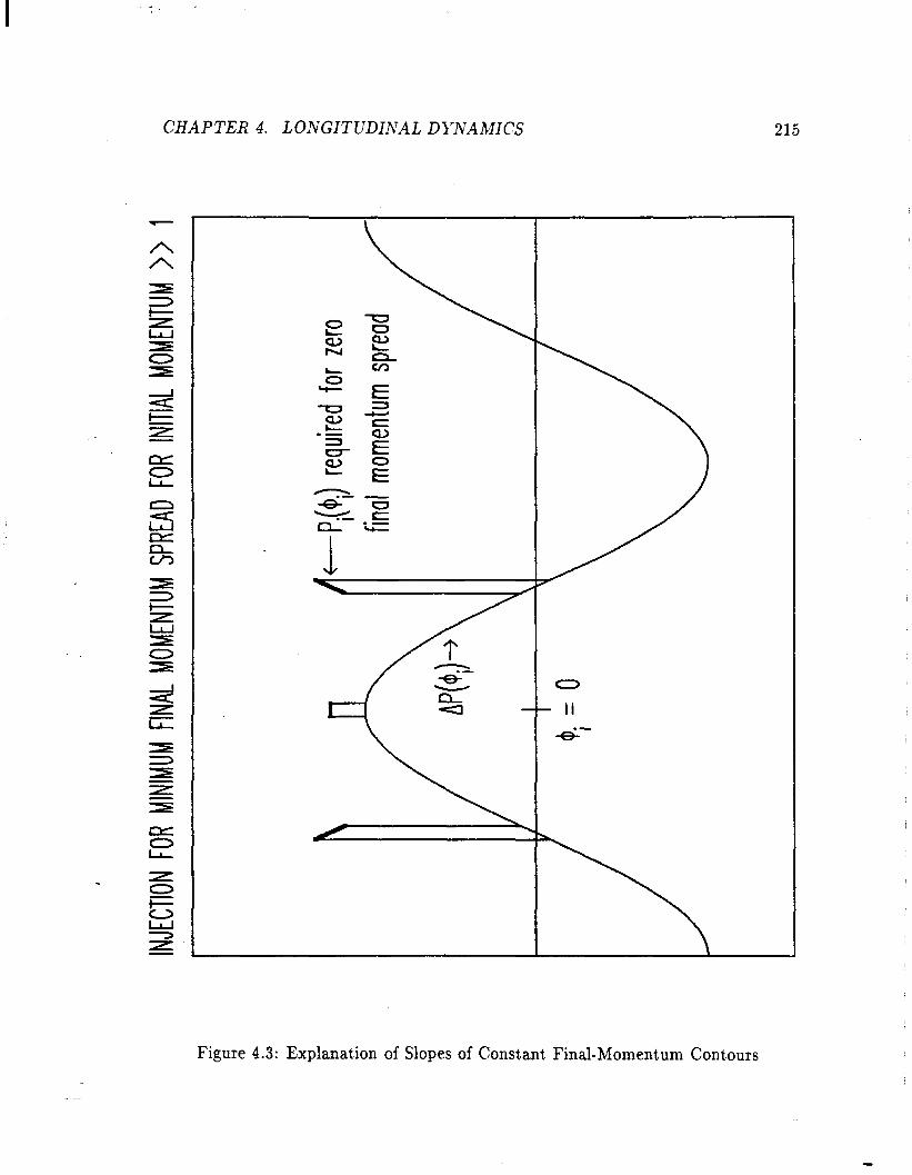
. __
INJE
CTKI
N FO
R MIN
IMUM
FI
NAL MOME
NTUM
SP
READ
FO
R INI
TIAL
MO
MENT
UM
>> 1

.
CHAPTER 4. LONGITtTDINAL DYNAMICS 216
region decreases at. the init,ial moment,um increases? since particles of higher init,ial
momentum loose less ve1ocit.y when decelerat,ed by the same fields, and evenhually
become capt,ured at. an accelerating phase.
Figure 4.2 gives additional insight into the longit.udinal dynamics. One sees t,hat,
the cont,our & = 0 lies in the region 4; 2 0, approaching & = 0 as pi increases. This
is because in order for a slow-moving particle to end up at & = 0, it. must, be in-
ject,ed ahead of the crest so that, the velocit.y-of-light. RF wave catches up t.o it as
it. becomes relativistic. This effect’ is less important, when t,he particle is initially
highly-relativist,ic, which is why the contour approaches @i = 0 as pi increases.
This Figure shows t,hab, by and large, in order t,o obtain a short. bunch, one must,
first. have a relatively short, bunch. The slight, slope to the constant, & cont,ours around
#+ = 0 indicat.es that, it, is best, to inject, the lower momentum part.icles ahead of t,he
higher-moment*um particles in OP bunch, so that. the former will fall back t,o t,he same
-phase as t’he later before the entire bunch becomes relativistic.
In order to get both a short’ bunch and a small final momentum spread, it is
necessary that one inject, t,he bunch along a constant, & cont,our in a region where
the constant. pf contours are widely spaced. Ideally, one would find two cont,ours, one
for constant $f and one for constant pf, t,hat. coincide over the required interval of pi,
and inject, one’s bunch witch the required phase-space distribution, c#+ vs pi.
Typical operat,ing conditions for the RF gun produce a peak moment8um of p = 5,
with momenta. down t,o p = 4 accept,ed (giving approximat,ely 3~10% moment,um
spread about. p = 4.5 for t,he “part,icles of int,erest,“). As was demonsbrat.ed in Chap-
ter 2, the higher moment’um particles exit the gun first, with the particles of int.erest,
occupying roughly 25 ps, or roughly 25” of S-Band phase. From the above discus-
sion, it. is clear that, this longitudinal phase-space dist,ribution must be alt,ered so that,
the higher-moment,um part.icles ent,er the linac after the lower-moment.um particles.
(The region #i > 90 is ruled out, because the particles are decelerated before being
accelerated, which is undesirable as it. would lead to increased space-charge effect.s.)
This can be accomplished by means of magnet,ic compression, as will be shown in the
next. section of this chapt.er. For present, purposes, I shall assume that t,he magnetic
compression syst,em can supply the desired moment,um-time correlat,ion: and at.tempt.
60 1ocat.e the opt’imum phase for inject,ion in order to get the smallest. final moment,um
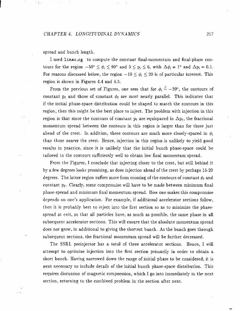
.
CHAPTER 4. LONGITUDINAL DE’NAhUCS 217
spread and bunch 1engt.h.
I used linac-cg to compute t,he const.ant’ final-momentmum and final-phase con-
tours for t,he region -50” 5 & 5 90” and 3 5 pi 5 6, wit,h A$; = 1” and Api = 0.1.
For reasons discussed below, the region -10 5 @i 5 20 is of particular interest. This
region is shown in Figures 4.4 and 4.5.
From 6he previous set of Figures, one sees that for +i z -2O”, the contours of
constant, pf and those of constant, $f are most’ nearly parallel. This indicat,es that.
if the initial phase-space distribution could be shaped t,o match the contours in this
region, then t,his might. be t.he best. place to inject. The problem with inject,ion in this
region is t.hat since t.he contours of constant, pf are equispaced in Apf, the fract.ional
momentum spread between the cont,ours in this region is larger than for t.hose just,
ahead of the crest. In addition, these cont,ours are much more closely-spaced in $i
than those nearer the crest. Hence, injection in t.his region is unlikely to yield good
results in pract,ice, since it. is unlikely that, the initial bunch phase-space could be
tailored to the contours sufficiently well t,o obdain low final momentmum spread.
From t.he Figures, I conclude that, injecting closer t.o the crest, but. still behind it
by a few degrees looks promising, as does injection ahead of the crest by perhaps 15-20
degrees. The lat,ter region suffers more from crossing of the cont,ours of constant $f and
constant pf. Clearly, some compromise will have t.o be made between minimum final
phase-spread and minimum final momenbum spread. How one makes this compromise
depends on one’s application. For example, if additional accelerat,or sections follow,
then it, is probably best, t,o inject, int,o the first, section so as t.o minimize t,he phase-
spread at. exit,, so that, all particles have, as much as possible, t,he same phase in all
subsequent’ accelerat.or sections. This will ensure that. the absolute momentum spread
does not grow, in addit,ional to giving the short,est. bunch. As the bunch goes through
subsequent, sections, the fracGona1 moment,um spread will be further decreased.
The SSRL preinjector has a total of three accelerabor sections. Hence, I will
at,tempt to opt,imize injecdion into the first section primarily in order to obtain a
short bunch. Having narrowed down t,he range of initial phase to be considered, it is
next necessary to include details of the initial bunch phase-space distribution. This
requires discussion of magnet,ic compression, which I go int,o immediately in the next.
section, returning t.o t,he combined problem in the section aft,er next.

1 -
218
CHAPTER 4. LONGITUDINAL DYlVAMICS
-- c! e
m
Pl Cm&
Figure 4.4: Expanded View of Const’ant, Find Moment,um Contours

-
Figure 4.5: Expanded View of Constant Final Phase Contours

.
CHAPTER4. LONGITUDINALDYNAMICS 220
4.2 Magnetic Bunch Compression
In the previous section I have shown t.hat, roughly speaking, what, one wants is t,o
deliver t.o t,he linac the short.est. possible bunch. More precisely, one wants a bunch
wit,h a longitudinal phase-space distribution at. the beginning of t,he linac that, will
be compressed further during initial acceleration. This depends upon being able
to reverse the time-order of electrons within each RF gun bunch, so t,hat’ the lowest.
moment,um particles ent.er the linac first and subsequently fall back to the same phase
as the highest momentum part.icles. Hence, a magnetic bunching syst,em will have t,o
be able t.o accomplish some degree of time-order reversal of particles in the bunch,
over a sufficient,ly large momentum interval. However, this is t.ypically only slightly
more difficult, that. producing a very short, bunch at, the ent,rance of t’he linac, and so
it, is convenient, to think in terms of how to produce a very short bunch. This allows
a separation of the problem of magnet’ic bunching from 6he details of longitudinal
dynamics in the linac: and hence prevents t,he issues from being obscured by too
much det,ail at. the out,set. Once the mechanism of magnetic bunching has become
clear, it, is then possible to go back and consider the effects of longit,udinal dynamics
in the first. part, of t,he linac.
4.2.1 First Order Solution for Bunch Compression
Consider, t.hen, that, it. is desired t,o produce a very short bunch at, the ent.rance of
the linac. It is known that, the bunches from t,he gun have a. particular moment.um
vs. exit’-time charact,eristic, namely, that. higher-moment,um electrons exit. the gun
ahead of lower-moment,um electrons. It. is convenient, to use the momentum deviat,ion,
6 - (P - Po)/Po, in t,erms of which, for a sufficiently small moment.um interval about’
the central moment.um p. G (Pr)o,
(4.17)
where texit refers to t,he t.ime of a particle’s exit from the gun and
(4.18)

.
CHa4PTER 4. LONGITUDINAL DYNAMICS 221
(Examination of the 1ongit.udina.l phase-space distribut,ions shown in previous chap-
ters shows that, for the &lo% moment’um spread that’ will be used, t.his linear ap-
proximation is not exact. However, it. is again not my purpose now to deal with this
det,ail, but, rat.her to explain t’he principle.) What is desired in order to have a very
short. bunch at, the end of the bunching syst,em is t.hat
tarrival = t,,it(b) + Ataight(S) = constant, (4.19)
where the subscript “arrival” refers t#o arrival at. the end of the bunching syst,em (i.e.,
t.he emrance bo the linac) and where I use At t ,fi&,t to indicat,e t,hat. the time-of-flight is
an int,erval rather t,han the time of some event. Combining these and using the linear
approximation of equation (4.17), I obtain
6 $ At,,,,,(b) = COnStant,
0
.-
and hence
From this last, equation and equation (4.18), one can see t,hat,
(4.21)
(4.22)
must be obtained at. the end of t,he bunching syst,em. In words, since higher mo-
ment,um particles come out, ahead of lower momentum part.icles, they must’ be put,
t.hrough a system in which the t,ime of flight is longer for high-moment.um particles
in order for all parbicles to arrive at the end at. the same time.
For particles that. are not, fully relativist,ic, time-of-flight depends upon bot,h ve-
1ocit.y and the length of the path taken
(4.23)
where s(6) represents t.he lengt,h of the path taken by a particle with moment,um
deviation 6. Since p = p/fip2 $ 1): it’ follows, t.o first order in 6, t.hat’
$=j$+(Po- o $)E. (4.24)
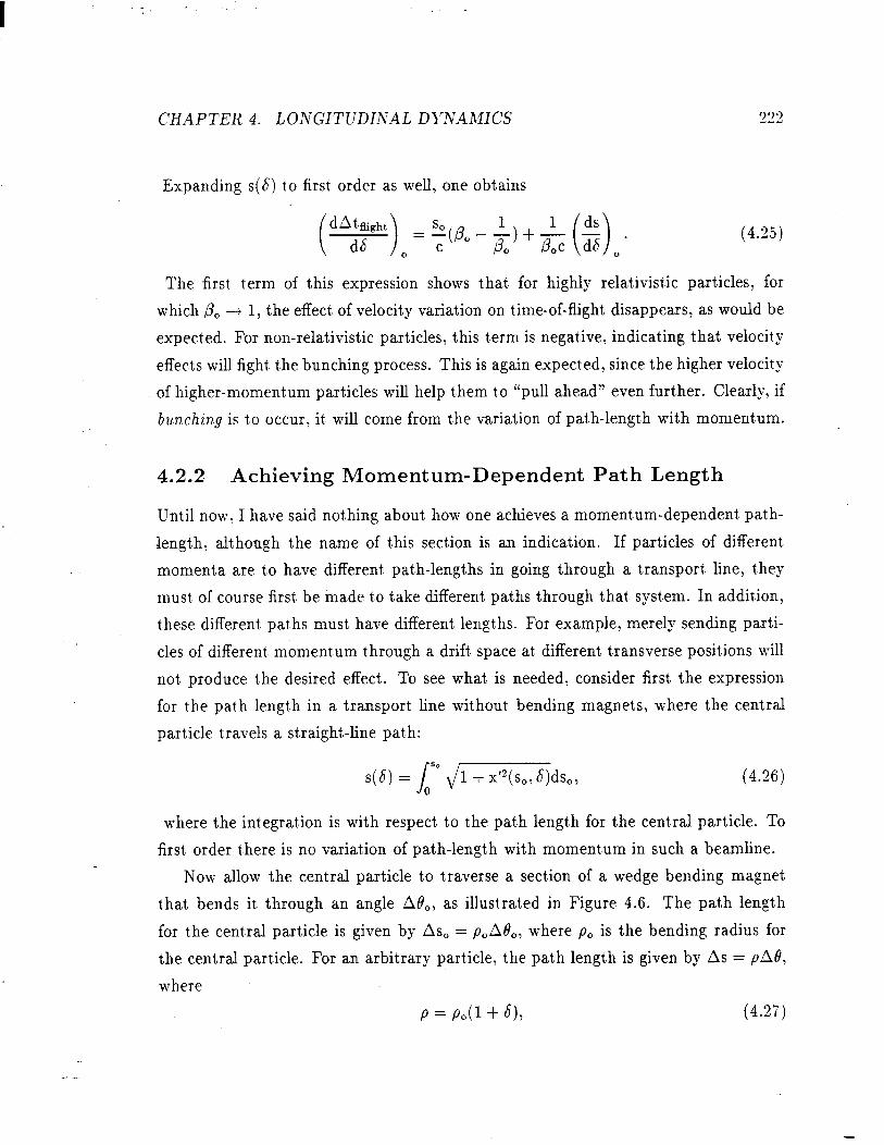
I .
CHAPTER 4. LONGITUDIIVAL DI’NAMCS 222
Expanding s(S) t,o first’ order as well, one obt,ains
=.iB,-$)+&($) . o c 0 0
(4.25)
The first. t,erm of this expression shows that, for highly relativistic part,icles, for
which PO -+ 1, the effect, of velociby variation on time-of-flight, disappears, as would be
expectSed. For non-relativist,ic particles, this t.erm is negative, indicating that. velocity
effects will fight. 6he bunching process. This is again expected, since the higher velocity
of higher-moment,um part,icles will help them to “pull ahead” even further. Clearly, if
bunchin,g is t,o occur, it will come from the variation of path-1engt.h with moment,um.
4.2.2 Achieving Momentum-Dependent Path Length
Until now, I have said not,hing about, how one achieves a momentum-dependent, pat’h-
lengt.h, although the name of t,his sect,ion is an indication. If particles of different
moment,a are to have different, path-lengt.hs in going through a transport line, they
must, of course first, be made bo take different, paths through that. system. In addit,ion,
these different pat.hs must. have different, lengt,hs. For example, merely sending part,i-
cles of different, momentum through a drift. space at, different, t,ransverse positions will
not, produce t,he desired effect. To see what, is needed, consider first the expression
for the pat.h lengdh in a transport, line without. bending magnets, where the cent,ral
particle t.ravels a straightline pat.h:
s(s) = J,‘” di%i$i&so, (4.26)
where the int,egrat,ion is wit.h respect to bhe pat,h 1engt.h for the cent.ral particle. To
first, order t.here is no variat,ion of path-length with momentum in such a beamline.
Now allow the central particle t,o traverse a sect.ion of a wedge bending magnet,
t,hat bends it through an angle AO,, as illust,rated in Figure 4.6. The path length
for the cent,ral particle is given by As, = p,AB,, where p. is the bending radius for
the central particle. For an arbitrary part*icle, the path length is given by As = ,oAB,
where
P = POP + 4, (4.27)

I-. P
P
t-4

CHAPTER 4. LONGITUDINAL DI’NAMICS 224
and where 8 is t,he angle the part,icle is bent. through in reaching the reference plane,
as illustrated in Figure 4.6.
Particles ot.her than the cent,ral part,icle will in general ent,er the bending magnet’
with different momenta, positions, and slopes relative to the central particle. Let’ xi
and xf be the initial position and slope of a particular particle, respectively. Some
trigonomet’ry reveals that. the angle through which an arbitrary particle is bent is
Ad = Ad, + atan + asin ysin(A8,) - sin [A#, + atan( . (4.28)
. . So far, no approximations have been made beyond assuming an ideal, hard-edge
magnetic field. In order t,o get, a first-order expression for the differential path-lengbh
in an infinitesimal section of a bending magnet, I expand t,o first,-order in Ad,, xi,
and xf, obtaining
As = pA6’ = A&(p, + x;). (4.29)
The init,ial coordinate xi is at, this point. arbitrary. I am int,erested, however, only
in moment,um-dependent, effect.s, and hence I will assume t,hat, the position of any
particle at. the entrance is a funct.ion only of its momentum, through t.he dispersion
function D, defined by
xi(S) = D6 + c3(S2). (4.30)
Hence, t:he differential path-lengt,h is
from which I conclude t,hat,
As = As& + (4.31)
(4.32)
(I use the total derivative because xi and xf are assumed to depend on S, i.e., t.his
quantit.y is not necessarily t.he mat,rix element rss (it, is equal to rss only when t.he
integrat,ion starts from a point’ where D=O). )
Referring back to equations (4.22) and (4.25), one sees that positive $ is required
for bunch compression. This is obtained when D and p have the same sign, which
is always t,he case for dispersion generat,ed within the magnet. itself (ot,herwise $
could be negat.ive for a lone bending magnet, which is absurd). I define the sign of D
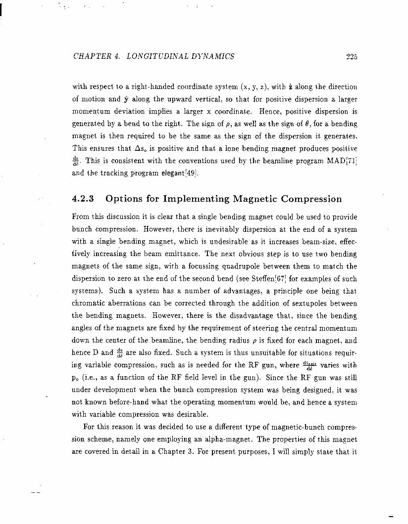
CHAPTER 4. LONGITUDINAL DYNAMICS 325
with respect. to a right’-handed coordinate system (x, y, z), wit,h i along the direction
of motion and jr along the upward vertical, so t,hat, for positive dispersion a larger
momentum deviation implies a larger x coordinate. Hence, positive dispersion is
generated by a bend to the right. The sign of p, as well as the sign of 8, for a bending
magnet is then required to be the same as t,he sign of the dispersion it, generates.
This ensures that. As, is positive and t.hat. a lone bending magnet, produces positive
$. This is consisdent, wit’h t.he convent,ions used by the beamline program MAD[71]
and t.he tracking program elegant [49].
4.2.3 Options for Implementing Magnetic Compression
From this discussion it is clear that, a single bending magnet could be used to provide
bunch compression. However, t,here is inevit,ably dispersion a6 the end of a system
wit.h a single bending magnet, which is undesirable as it, increases beam-size, effec-
tively increasing the beam emit,tance. The next, obvious step is t,o use two bending
magnets of the same sign, wit’h a focussing quadrupole bet,ween them to match the
dispersion to zero at, t,he end of the second bend (see Steffen[67] for examples of such
syst,ems). Such a system has a number of advantages, a principle one being that.
chromatic aberrations can be correct,ed through the addition of sext.upoles between
the bending magnets. However, there is the disadvantage that., since the bending
angles of t’he magnets are fixed by the requirement, of st,eering the cent,ral momentum
down t.he center of the beamline, the bending radius p is fixed for each magnet, and
hence D and g are also fixed. Such a syst,em is thus unsuitable for situations requir-
ing variable compression, such as is needed for the RF gun, where * varies with
pO (i.e., as a function of the RF field level in the gun). Since the RF gun was still
under development when the bunch compression system was being designed, it was
not. known before-hand what the operating moment.um would be, and hence a system
with variable compression was desirable.
For this reason it was decided to use a. different. type of magnetic-bunch compres-
sion scheme, namely one employing an alpha-magnet. The propert’ies of t,his magnet
are covered in detail in a Chapt,er 3. For present. purposes, I will simply state that it,
--

CHAPTER 4. LONGITUD.lNilL DYNAMICS 226
is firsCorder a,chromat’ic but’ has moment,um-dependent pabh-length described by
~a@‘> = K, (4.33)
where s is in meters, g is the gradient, in G/cm, K, = 1.91655, and, as above,
p0 = (PT)~. From th is, it is seen that for t,he alpha-magnet,
(4.34)
Like bending-magnet,-based schemes, an alpha-magnet. provides momentum-dependent.
path-lengt,h because of bending and t,he result.ant dispersion. However since t#he alpha-
magnet. is a gradient, magnet, t,he bending radius varies wit,h positsion along t,he cent,ral
t,ra.jecbory. The alpha-magnet has the advant,age t,hat. 6he gradient, and hence %,
can be varied without. changing the central trajecdory outside of t,he alpha-magnet.
While t,here are ot,her syst.ems wit,h this propert’y[72], t.he alpha-magnet, is probably
the simplest. - It. also has the advantage of relat.ively small aberrations, but has the
disadvantage that, t.here is no simple way to incorporate sext,upoles for correction of
chromatic aberrations in ext,ernal quadrupoles that might, be required as part, of the
beamline.
EvaluaCng (4.33) for 6 = 0, and inserting bhe result, along with equation (4.34)
into (4.25), and thence int.o (4.22), I obtain Qhe requirement, for bunching
f (KffE+L&ift) (BcI-+-) +j$f-/f= -!.!Z$, (4.35)
where I have used
s(S) = Ldrift + Sa(b) (4.36)
t,o incorporat,e the effects of any drift. spaces bet,ween the gun and alpha-magnet, and
bet.ween t,he alpha,-magnet. and linac. It’ will prove useful to group the alpha-magnet,
terms together, as in
Solving for the gradient,, I obtain
g= PZ: (A - &-)’
[ C* + L&ift (A - k)]”
(4.37)
(4.38)

CHAPTER 4. LONGITUDINAL DYNAMICS 22T
This equation reveals a number of aspects of bunch-compression with an alpha-
magnet. Since % < 0 and PO - & < 0, the denominator will be zero only if Ldrift = 0
and the initial bunch has zero length, i.e., only if bunching is not. needed. One also
sees that, the longer the drift. spaces, the lower the alpha-magnet. gradient, must. be,
in order to compensat,e for the debunching.
The t,erm (Do - $-,, in the numerator combines the effects of debunching in
t,he alpha-magnet, due to differential ve1ocit.y with that, of bunching in the alpha-
magnet. due to differential pat,h-length. Not,e that, the solut,ion (4.38) is not. valid for
PO < l/d, since t,hen all t’erms on the left,-hand side of (4.37) are negative. Hence,
for PO < l/d, the alpha magnet, cannot bunch, as t,he effects of velocit*y variation will
always overcome the effect.s of path-length variat(ion. (This is false only if % > 0,
a sit,uation that. does not. apply for the RF gun.)
Taking the limit’ of equat,ion (4.38) as PO --+ 1, one obtains
. . ~3:
L21 g = (2cd+)2 ’ (4.39)
which indicat,es that. for constant. bunch 1engt.h and constant fractional moment’um
spread (implying constant *), the gradient. must’ increase with increasing central
momentum. If, however, the &sol&e momentum spread is kept constant. (as hap-
pens wit’h accelerat,ion of relat,ivistic particles near the crest of the RF field), then
* scales as pO, which indicates that t.he gradient, must scale inversely with momen-
t,um. A smaller gradient implies a larger alpha magnet, since t,he size of the cent.ral
traject.ory scales as l/d (see Chapt,er 3). Hence, bunching before acceleration is ad-
vantageous in that, it decreases the size of the alpha-magnet, at, the cost, of requiring a
higher gradient. Similarly, as p, * l/fifrom PO > l/a, the gradient must. become
vanishingly small, implying a increasingly large alpha-magnet.

CHAPTER 4. LONGITIJDINAL DYNAMICS 228
4.3 Optimized Bunch Compression for the RF
Gun
In the previous two sections, I discussed the principles that, must, be employed in
choosing t,he injection phase and t,he alpha-magnet, gradient for production of short,
bunches with low final moment,um spread. I att*empted to separate t,he t,wo aspects,
for simplicit’y in the discussion. In this section, I demonstrate how bo obtain opt.imum
performance wit*h simultaneous consideration of accelerabion and magnetic bunching,
along with inclusion of the det,ailed initial phase-space. Not’ surprisingly, this opt,i-
mization is best, done numerically.
I have written a program, alpha-opt, that. accept,s initial longitudinal phase-space
information in t,erms of (&,pi) pairs for macro-particles (e.g., from MASK or rfgun)
and att.empts t,o find the optimum alpha-magnet gradient for a specified accelerat,or
phase and energy gain. It. opt,imizes for eit’her the minimum mean absolute phase
deviation or t’he minimum total phase-length of the final bunch, though I have used
the latter crit#erion exclusively in this work. Equation (4.33) is used witChout, approx-
imation in (4.36) bo give the moment,um-dependent. path-length. Equation (4.1) is
used for the traveling wave field. To simulat,e particle motion in the accelerat,or, I
employ equations (4.2) and (4.3) (scaled for more efficient, computation), which I in-
tegrate using the so-called “leap-frog” met,hod[61], which is second-order accurat.e in
t*he t,ime-st,ep. Typically, I find that taking time-steps smaller t,han 30 ps makes no
change in t,he result,s (i.e., no change of more t,han 1O.OOlps in the bunch length).
4.3.1 Use of alpha-opt to Optimize Bunch Compression
The combined distance, Lhift, from the gun t.o t,he alpha-magnet, and from the alpha-
magnet, to the tender of the first, linac cell (where the traveling wave begins) was
chosen based on simulat,ions of the gun longitudinal phase-space, the anticipated
st,rength and good-field-region of the alpha-magnet., and t,he need for a sufficiently
long drift,-space t.o accommodat,e the quadrupoles and chopper. Because the gun was
still under development at, t,he t,ime t,he alpha-magnet and GTL were being specified,
I chose Ldrift so t,hat compression would be feasible over a wide range of gun operating

CH,4PTER 4. LONGITUDIN.4L DYNAMICS 229
momenta, rather t.han finding an optimum for any part.icular beam momentum. If
L&if, were chosen t.o be too short, then an excessively strong alpha-magnet, would be
needed in order to reduce the compression, while if L&if, were chosen bo be too long, an
unreasonably large good-field region would be needed to provide more compression.
Ldrift = 1.5m was initially chosen based on preliminary simulations with rfgun and
alpha-opt, along with knowledge of the (then preliminary) magnetic design of the
alpha-magnet,. Lat,er, L drift was increased to 1.7m in order t’o provide more space for
other GTL components.
More specifically, there is a 0.6m drift, space from the gun to the alpha.-magnet’
crossing point, and a l.lm drift’ from the alpha-magnets to t.he linac. See Chapter 5
for more discussion of the layout, of the GTL.
I performed a series of alpha-opt runs st.arting wit,h t.he MASK-generated lon-
git,udinal phase-space dist,ribution for the RF gun operat,ed at, Ep2 = i5MV/m and
J = lOA/cm 2. The linac simulation parameters were such that an initially relat,ivis-
tic particle injected at, t,he crest, would gain 45 MeV (which corresponds to 20.7
MW RF power). I took the highest.-moment8um part,icle as the fiducial particle, and
chose to at,tempt’ to compress the beam for a variet,y of momentum spreads, name-
ly ilO%, is%: and &2.5%. That’ is, I applied a perfect momentum-filter to the
MASK-generat,ed beam, accept.ing only particles such t,hat p,(l - f) 5 p < p,(l + f),
with p; - pmax/(l + f), where if is the fract,ional momentum spread accepted. In
this way, the selected momendum range always cont,ains the highest moment,um par-
t,icles. (This same capabilit.y exists on the actual beamline, where a scraper inside
the alpha-magnet, can be moved into the beam from the low-moment,um side.)
For each value of f, I first. found the alpha-magnet, gradient. which produced the
shortest bunch at the ent#rance to the linac. I then used this gradient, and sent’ the
bunch down the linac with the highest’-moment,um particle injectsed at. the crest, fully
expecting that, the result, would be a less than optimally compressed bunch. The
simulations confirmed this expectat,ion, as the data listed in Table 4.1 shows. (In this
and all subsequent, Tables and Figures, At’ and AP are the full spread of the values,
e.g., At. = t,,, - tbn.) In addit,ion, one sees t,hat. the absolute moment. spread has
increased. The phase-space dist,ributions at. t,he linac ent.rance and exit are represended
graphically in Figure 4.7. Not.e that’ these graphs are of time and moment.um: rather
--
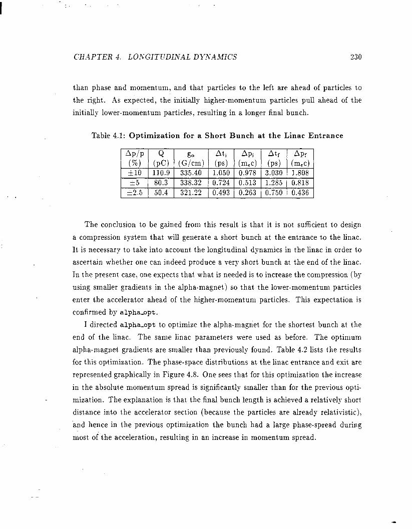
7
CHAPTER 4. LONGITUDINAL DIrNAhUCS 230
t,han phase and moment,um, and that. particles t.o t,he left are ahead of particles to
the right. As expecbed, t,he initially higher-moment.um particles pull ahead of the
initially lower-momentSum particles, result.ing in a longer final bunch.
Table 4.1: Optimization for a Short Bunch at the Linac Entrance
APIP & APi An (%) (PC) (G$zm) ii\ (m,c) t”s; (m,c) 110 110.9 335.40 1.050 0.978 3.030 1.808
15 80.3 338.32 0.724 0.513 1.285 0.818
12.5 50.4 321.22 0.493 0.263 0.750 0.436
The conclusion to be gained from this result is that, it is not sufficient, t,o design
a compression system that. will generat.e a short, bunch at, t,he entrance t,o t,he linac.
It’ is necessary to take into account, the longitudinal dynamics in t,he linac in order t.o
ascert,ain whether one can indeed produce a very short bunch at, the end of the linac.
In t,he present, case, one expects that’ what. is needed is t,o increase the compression (by
using smaller gradients in the alpha-magnet,) so that. the lower-momentum particles
enter the accelerat,or ahead of the higher-moment$um particles. This expectat.ion is
confirmed by alpha-opt.
I direct,ed alpha-opt to optimize t’he alpha-magnet. for the shorbest. bunch at tShe
end of t.he linac. The same linac parameters were used as before. The opt.imum
alpha.-magnet gradients are smaller than previously found. Table 4.2 lists 6he results
for this optimization. The phase-space dist,ributions at the linac entrance and exit. are
represented graphically in Figure 4.8. One sees t,hat, for this opt,imizat,ion t.he increase
in t,he abso1ut.e moment,um spread is significantly smaller than for the previous opti-
mizat,ion. The explanation is that the final bunch length is achieved a relatively short
distance into t.he accelerat,or section (because t,he particles are already relativistic),
‘and hence in the previous optimization the bunch had a large phase-spread during
most, of the acceleration, resulting in an increase in momentum spread.
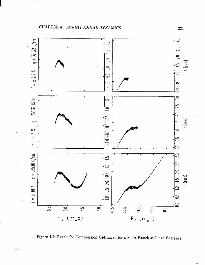
CHd4PTER 4. LONGITUDINAL DYNAMICS 231
-” -
+@@ :,. ,.. . . 0 4
/ -LT!
11 0 d
-I I -r
;s: -9 N U-7 -
-9
-”
II 4 CT,
ho 0, - -i-i II
_.
‘i Crnec> p, b-p>
Figure 4.7: Result for Compression Optimized for a Short. Bunch at. Linac Ent,rance
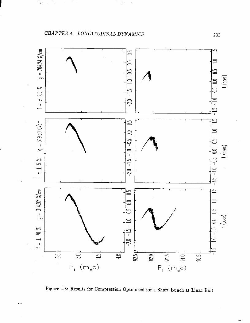
CHAPTER 4. LONGIT/JDINAL DYNAMICS 232
Figure 4.8: Results for Compression Opt,imized for a Short Bunch at Linac Exit
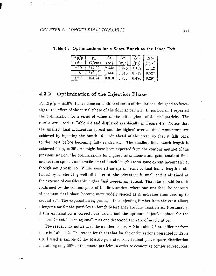
CHAPTER 4. LONGITUDINAL DYNAMICS 233
Table 4.2: Optimizations for a Short Bunch at the Linac Exit
I AP/P I g, I Ati I APi I At, I APf I
4.3.2 Optimization of the Injection Phase
For Ap/p = IlO%: I have done an additional series of simulations, designed to inves-
tigat,e t,he effect. of the initial phase of t,he fiducial particle. In particular, I repeat,ed
the opt,imization for a series of values of the initial phase of fiducial particle. The
results are listred in Table 4.3 and displa.yed graphically in Figure 4.9. Notice that
the smallest final momendum spread and the highest, average final momentum are . . achieved by injecting the bunch 10 - 15” ahead of the crest, so that it falls back
to the crest, before becoming fully relativistic. The smallest final bunch length is
achieved for $+, = 20”. As might have been expected from the contour method of bhe
previous section, the optimizations for highest total momentum gain, smallest, final
momentum spread, and smallest final bunch length are to some extent. incompatible,
though not, grossly so. While some advantage in terms of final bunch length is ob-
tained by accelerat,ing well off the crest,, the advantage is small and is obtained at,
the expense of considerably higher final moment.um spread. That this should be so is
confirmed by the contour-plots of the first. section, where one sees that the contours
of constant final phase become more widely spaced as @I increases from zero up to
around 90”. The explanation is, perhaps, that injecting further from t.he crest allows
a longer time for t,he particles to bunch before they are fully relativistic. Presumably,
if this explanation is correct, one would find the optimum injection phase for t,he
shortest, bunch becoming smaller as one decreased the rate of acceleration.
The reader may notice that bhe numbers for 4. = 0 in Table 4.3 are different. from
those in Table 4.2. The reason for this is that for the optimizations presentfed in Table
4.3, I used a sample of the MASK-generated longit.udinal phase-space distribution
containing only 20% of t,he macro-particles in order to economize computer resources,
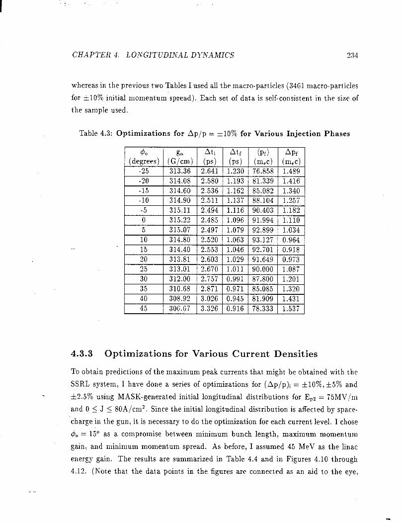
-
CHAPTER 4. LONGITUDINAL DYh’AMICS 234
whereas in the previous t,wo Tables I used all t’he macro-part.icles (3461 macro-part.icles
for ilO% init,ial momentum spread). Each set. of data, is self-consistsent, in the size of
bhe sample used.
Table 4.3: Optimizations for Ap/p = AlO% for Various Injection Phases
4.3.3 Optimizations for Various Current Densities
To obtain predictions of bhe maximum peak currents that. might. be obtained with the
SSRL system, I have done a series of optimizations for (Ap/p)i = &lo%, &5% and
12.5% using MASK-generat,ed initial longit,udinal distributions for Ep2 = 75MV/m
and 0 5 J 5 80A/cm2. Since the initial longitudinal distribut.ion is affect,ed by space-
‘charge in bhe gun, it is necessary to do the opt,imizat,ion for each current level. I chose
& = 15” as a compromise bet,ween minimum bunch length, maximum momentum
gain, and minimum moment,um spread. As before, I assumed 45 MeV as the linac
energy gain. The results are summarized in Table 4.4 and in Figures 4.10 t,hrough
4.12. (Not.e that. the dat.a point.s in t.he figures are connected as an aid to the eye,
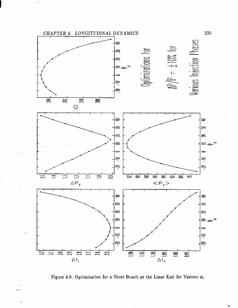
CHAPTER 4. LONGITUDINAL DZ’NAMCS 235
Figure 4.9: OptimizaGon for a Short. Bunch at the Linac Exit for Various &
--

-
CHAPTER 4. LOiVGITUDINAL DE’XAMICS 236
and not, bo indicat,e any assumed variat,ion in t,he quant’ities bet,ween dat,a points.)
Table 4.4: Optimizations for Various Cathode Current Densities
(Ap/p), = &lo%
At f,mad (Pf) Apf APf,mad Q (1) (~4 b-4 b-4 b-4 (PC) A
4.3.4 Effects of Transport Aberrations
These predict,ions of high peak current,s neglect, space-charge forces in the gun-t,o-linac
transport, line and in t#he linac itself. They also neglect, the effects of non-chromatic
t5jk and u5jM terms (“aberrations”) in the alpha-magnet,, and of field errors in t.he
alpha-magnet. (see Chapter 3). Other effect,s that. are not. included in the analysis are
wake-fields in the accelerat,or sect,ion. In Chapter 3, I discuss the effect. of field errors,
and show t,hat the effect of field errors on r5j mat.rix elements is small, from which I
conclude t,hat. the abi1it.y of t,he alpha-magnet’ to compress the bunch is unaffect,ed by
field errors.
To evaluate t,he effects of space-charge, both in the GTL and in t,he accelerat,or

.
CHAPTER 4. LONGITUDINAL DYNAMICS 237
I I I I I I I I I
. . I pcra‘k CA)
I I I I I I I I I I I I I - I -
-63 -63
-e -e
-s -s
-53 -53
-s -s
-53 -53
0 0
0 0
I I I I I I I I I I I I 1 O 1 O
AP, <m,c>
Q <PC)
I I I I
-ss
-E
-kz
-53
-z
43
-El
0
0 I I I I
x 8 Ln 0 - - w . e
- - - -
At, CPS)
Figure 4.10: Results of Optimized Compression for Various Cathode Current, Densi- ties, for (AP/P)i = &lo %

-
CHAPTER 4. LONGITUDINAL DYNAMICS 238
I I I I I I
-s -s
-e -e
-53 -53
-sa -sa
-0 -0
-E -E
-Ei -Ei
0 0 - -
_. 1 peak CA)
-52
-e
-z
33
Q <PC)
I I I I I ‘
-z 2 a
APT (m-c) At, CPS>
Figure 4.11: Results of Opt.imized Compression for Various Cathode Current Densi- ties, for (AP/P)i = f5 %

CHAPTER 4. LONGITUDINAL DYNAMICS 239 I I I I I I I
-1
-s
-e
-s
-s
Figure 4.12: R.esu1t.s of Optimized Compression for Various Cathode Current, Densi-
ties, for (AP/P)i = f2.5 %
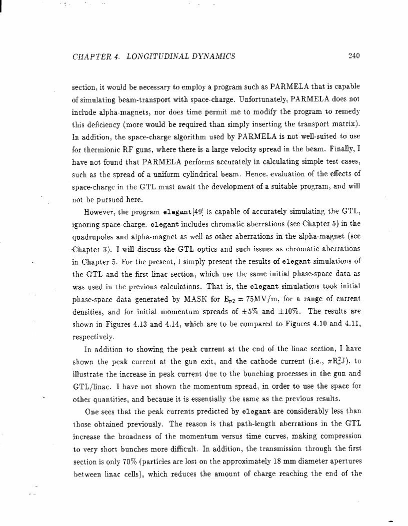
.
GHAPTER4. LONGITUDINAL DlrhrAMICS 240
section, it would be necessary t,o employ a program such as PARMELA that, is capable
of simulating beam-transport. with space-charge. Unfortunately, PARMELA does not,
include alpha-magnets, nor does time permit. me to modify t.he program to remedy
this deficiency (more would be required than simply inserding the t,ransport mat’rix).
In addition, the space-charge algorithm used by PARMELA is not, well-suited t,o use
for thermionic RF guns, where t,here is a large velocity spread in the beam. Finally, I
have not. found that, PARMELA performs accurately in calculat.ing simple test. cases,
such as the spread of a uniform cylindrical beam. Hence, evaluation of the effect,s of
space-charge in the GTL must, await, the development, of a suitable program, and will
not, be pursued here.
However: the program elegant[49] is capable of accurat,ely simulating the GTL,
ignoring space-charge. elegant includes chromat,ic aberrations (see Chapter 5) in the
quadrupoles and alpha-magnet as well as other aberrations in the alpha-magnet (see
Chapter 3). I will discuss the GTL optics and such issues as chromatic aberrations
in Chapt,er 5. For the present, I simply present the results of elegant simulations of
t,he GTL and the first’ linac section, which use tshe same initial phase-space data as
was used in the previous calculations. That, is, the elegant simulations took initial
phase-space data generat,ed by MASK for Ep2 = 75MV/m, for a range of current
densities, and for initial momentum spreads of &5% and &lo%. The result,s are
shown in Figures 4.13 and 4.14, which are to be compared to Figures 4.10 and 4.11,
respectively.
In addition bo showing t,he peak current, at the end of the linac section, I have
shown the peak current, at the gun exit, and the cathode current (i.e., nR:J), to
illust.rat,e t#he increase in peak current due to the bunching processes in 6he gun and
GTL/linac. I have not shown t,he momentum spread, in order t.o use t.he space for
other quant.it,ies, and because it, is essentially the same as the previous results.
One sees that the peak currents predicted by elegant are considerably less t’han
those obt.ained previously. The reason is that path-length aberrations in the GTL
increase the broadness of t,he momentum versus time curves, making compression
t,o very short bunches more difficult. In addit,ion, the transmission through the first
section is only 70% (part,icles are lost. on t,he approximately 18 mm diameter apert,ures
between linac cells), which reduces t,he amount, of charge reaching the end of the

CHAPTER 4. LONGITUDINAL DYNAMICS
* . . .
i I I I I
Figure 4.13: elegant/MASK Results after First. Accelera.tor Section, for Various Cat.hode Current Densities and Ep2 = 75MV/m, for (AP/P)i = &lo %

-
CHAPTER 4. LONGITUDINAL D'1'NAMICS
_. At, - (PS)
P 4 _, ,.A . . .:’
a
0 m 0 C’
E (7-T m,c wm>
-I
I ,
I
Ez 0
I pea: (A)
e
‘,,, i, I
i 0 ‘I
B
8” <A/mm2/mr2)
Figure 4.14: elegant/MASK Results after First, Accelerator Section, for Various Cathode Current. Densities and Ep2 = 75MV/m, for (AP/P); = k5 %

I
CH.4PTER 4. LONGITUDIhlAL DYNAMICS -1 I I I
1 I I I I I
*./
I I I I
q 9 Lc 9 - -
_. At, -(Ps)
I I I I
7% \,,, -
\
5 - -
‘\
i \
f
u7 Y
m,c lum>
I I I I I
z 0 h
I PRO;;- (A>
I I I
z
‘. ‘a.. ir3
5 “i ‘\
z =_., w . . ...“ m -.. Y_,
I I I
N - v
-1 I
,t I
,
I
d
, I
, I
0
s
243
RI (A/mm2/mr2)
s
Figure 4.15: Longit.udinal Phase-Space at, Various Points in the GTL (elegant/MASK results for E,,Z = 75MV/m, J = lOA/cm’, and (AP/P)i = &lo %).
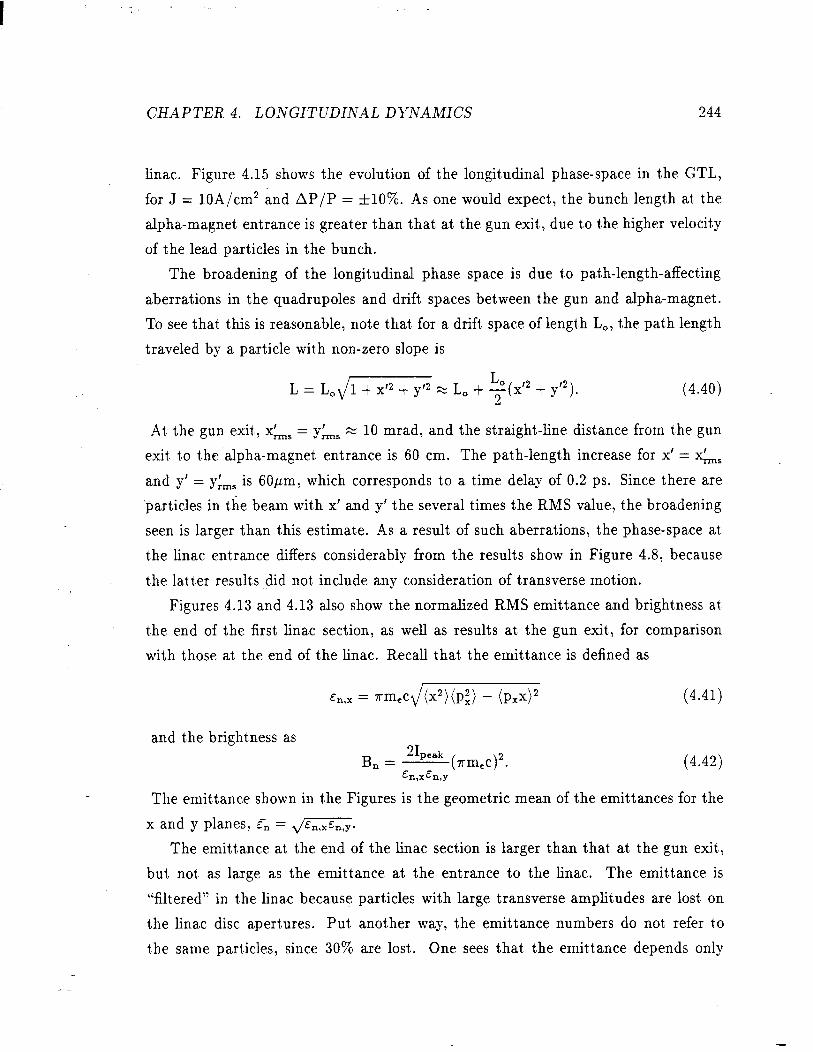
.
CHAPTER 4. LONGITUDIhrAL DYNAMICS 244
linac. Figure 4.15 shows the evolution of the longit,udinal phase-space in the GTL,
for J = 10A/cm2 and AP/P = &lo%. As one would expect, the bunch length at’ the
alpha-magnet, enkance is greater than that at, the gun exit, due to the higher ve1ocit.y
of the lead particles in the bunch.
The broadening of the longitudinal phase space is due to path-length-affecting
aberrations in the quadrupoles and drift, spaces bet,ween the gun and alpha-magnet.
To see that’ t,his is reasonable, not,e that for a drift. space of lengt,h L,, the pat.h length
traveled by a particle wit.h non-zero slope is
L=L,dW=Lc+ +(xr2 + y’“). (4.40)
At’ the gun exit,, &, = y&, z 10 mrad, and the st,raight,-line distance from the gun
exit, t,o the alpha-magnet ent,rance is 60 cm. The pabh-length increase for x’ = &,
and y’ = y:,, is 60pm, which corresponds to a time delay of 0.2 ps. Since there are
particles in the beam with x’ and y’ t.he several times the RMS value, the broadening
seen is larger than this estimate. As a result. of such aberrations, the phase-space at
the linac ent,rance differs considerably from t.he results show in Figure 4.8, because
the latt.er results did not, include any consideration of transverse mot’ion.
Figures 4.13 and 4.13 also show the normalized RMS emittance and brightness at,
the end of the first linac section, as well as results at, the gun exit, for comparison
with those at, the end of the linac. Recall that. the emittance is defined as
& - rmec (x2)(pf) - (PG)* n,x - (4.41)
and the brightness as
B, = 2I,e,k
-(7rm,c)2. (4.42) & & n,x n,Y
The emittance shown in t,he Figures is the geometric mean of the emittances for the
x and y planes, fn = d-.
The emitt,ance at the end of the linac sectlion is larger than that, at, the gun exit,
but, not. as large as the emittance at. the entrance t,o the linac. The emittance is
“filtered” in the linac because particles with large transverse amplit,udes are lost on
the linac disc apert,ures. Put. anot.her way, t#he emittance numbers do not, refer to
t,he same part.icles, since 30% are lost,. One sees that, the emittance depends only
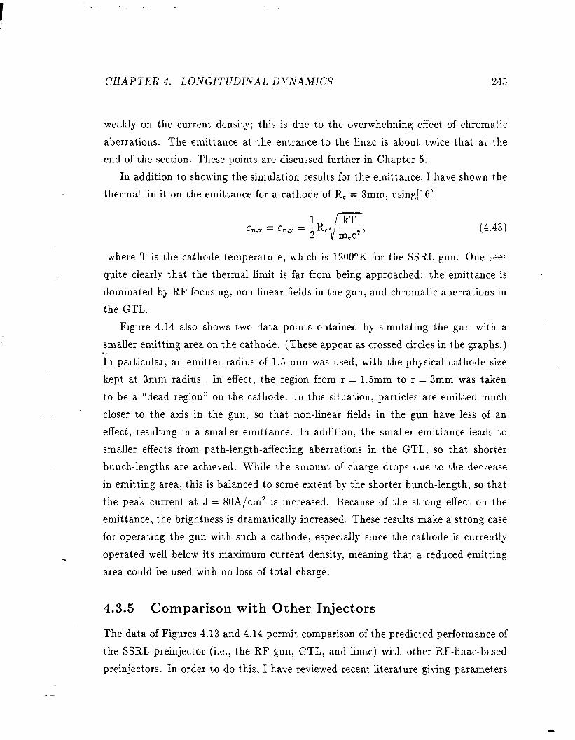
.
CH.4PTER 4. LONGITUDINAL D~‘NAiWCS 245
weakly on the current, densit’y; t,his is due to the overwhelming effect of chromatic
aberrations. The emittance at, the ent.rance to the linac is about. twice that, at t.he
end of the section, These points are discussed further in Chapter 5.
In addition t,o showing the simulation results for the emit,tance, I have shown t.he
thermal limit on the emit,tance for a cathode of R, = 3mm, using[l6]
& -& n,x - n,Y = (4.43)
where T is the cat(hode temperat,ure, which is 1200°K for the SSRL gun. One sees
quite clearly t&hat. t,he thermal limit, is far from being approached: the emittance is
dominat.ed by RF focusing, non-linear fields in the gun, and chromatic aberrations in
t,he GTL.
Figure 4.14 also shows t.wo data points obtained by simulat.ing the gun with a
smaller emitting area on t,he cat,hode. (These appear as crossed circles in t,he graphs.) _. In particular, an emitter radius of 1.5 mm was used, with the physical cathode size
kept’ at, 3mm radius. In effect, the region from r = 1.5mm to r = 3mm was taken
to be a “dead region” on the cathode. In this situation, part.icles are emitted much
closer to the axis in t,he gun, so that, non-linear fields in the gun have less of an
effect, resulting in a smaller emit,tance. In addition, the smaller emit*tance leads t,o
smaller effects from path-length-affecting aberrat’ions in the GTL, so t.hat, short,er
bunch-lengt.hs are achieved. While t,he amount. of charge drops due to the decrease
in emibting area, this is balanced t.o some ext,ent# by the shorter bunch-lengt,h, so that
t’he peak current, at, J = 80A/cm2 is increased. Because of bhe strong effect. on t,he
emitbance, the brightness is dramatically increased. These results make a strong case
for operating the gun with such a cathode, especially since the cathode is currently
operated well below its maximum current densit(y, meaning that. a reduced emit,ting
area could be used with no loss of t,otal charge.
4.3.5 Comparison with Other Injectors
The data of Figures 4.13 and 4.14 permit, comparison of the predict,ed performance of
t,he SSRL preinject,or (i.e., the RF gun, GTL, and linac) with other RF-linac-based
preinjectors. In order t(o do this, I have reviewed recent’ lit,erat,ure giving parameters
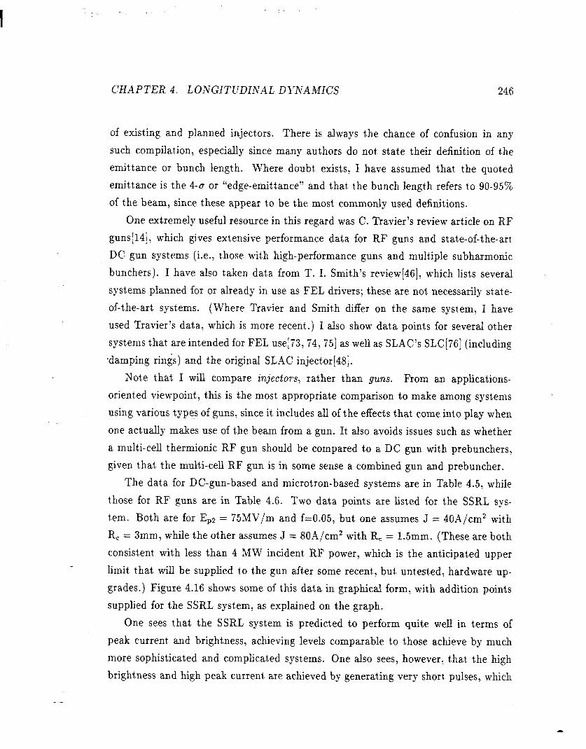
CHAPTER 4. LONGITUDINAL DYNAMICS 246
of existing and planned injectors. There is always the chance of confusion in any
such compilat,ion, especially since many authors do not. stade their definition of the
emit*tance or bunch length. Where doubt’ exists, I have assumed thad the quoted
emittance is the 4-u or “edge-emittance” and that, t.he bunch 1engt.h refers Qo 90-95%
of the beam, since these appear t.o be the most, commonly used definitions.
One extremely useful resource in this regard was C. Tra.vier’s review article on RF
guns[l4], which gives extensive performance data for RF guns and stat,e-of-the-art
DC gun systems (i.e., those wit,h high-performance guns and multiple subharmonic
bunchers). I have also t,aken data from T. I. Smith’s review[46]? which lists several
syst,ems planned for or already in use as FEL drivers; these are not. necessarily st.at,e-
of-t’he-art’ systems. (Where Travier and Smith differ on the same syst.em, I have
used Travier’s data, which is more recent.) I also show data points for several other
syst.ems that, are intended for FEL use[73, 74, 75j as well as SLAC’s SLC[76] (including
-damping rings) and the original SLAC injector[48].
Not.e that, I will compare injectors, rather than guns. From an applications-
orient.ed viewpoint, t,his is the most appropriate comparison to make among systems
using various types of guns, since it includes all of the effects that. come into play when
one actually makes use of t,he beam from a gun. It also avoids issues such as whether
a m&i-cell thermionic RF gun should be compared to a DC gun with prebunchers,
given t,hat. the mult,i-cell RF gun is in some sense a combined gun and prebuncher.
The dat,a for DC-gun-based and microtron-based systems are in Table 4.5, while
those for RF guns are in Table 4.6. Two daba. points are listed for the SSRL sys-
hem. Both are for Ep2 = 75MV/m and f=0.05, but one assumes J = 40A/cm2 with
R, = 3mm, while the other assumes J = 80A/cm2 with R, = 1.5mm. (These are both
consist,ent, with less than 4 MW incident. RF power, which is the anticipabed upper
limit that, will be supplied t,o the gun aft,er some recent,, but. unt,ested, hardware up-
grades.) Figure 4.16 shows some of this data in graphical form, with addition points
supplied for the SSRL system, as explained on bhe graph.
One sees dhat, the SSRL system is predicted to perform quite well in terms of
peak current, and brightness, achieving levels comparable to those achieve by much
more sophisticated and complicated systems. One also sees, however, that. the high
brightness and high peak current. are achieved by generat,ing very short, pulses, which
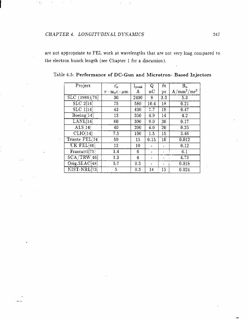
CHAPTER 4. LONGITtlDINAL DYNAMICS 247
are not. appropriat,e t,o FEL work at, wavelengt,hs that, are not’ very long compared t.o
t,he elect,ron bunch length (see Chapter 1 for a discussion).
Table 4.5: Performance of DC-Gun and Microtron- Based Injectors
Project. G I peak Q 6t B,
7r-rnm,c-tirn A nC DS A /mm2 /mr2 I 1 SLC (1986)/761 1 io 1 1 2400 1 8 1 3.3 1 ’ 5.3’
I I I I
SLC 2[14] I 75 580 10.4 18 0.21 SLC 1[14] 43 430 7.7 19 0.47 Boeing [ 141 13 350 4.9 14 4.2 LANL/141 60 300 9.0 30 0.17 ALSli41- 40 I 200 I 4.0 I 20 I 0.25
t CLIdll41 I I I I I
7.5 I 100 I 1.5 I 15 I 3.46 I 1 Trieste F’Eil741 1
I I I I 50 I 15 I 0.15 I 10 I 0.012
UK FEL[46j _ 13 10 - - 0.12 Frascat,ti[75] 1.4 6 - - 6.1
SCA/TRW[46] 1.3 4 - - 4.73 Orig.SLAC[48] 5.7 0.3 - - 0.018 NIST-NRLl73i 5 0.3 14 15 0.024
--
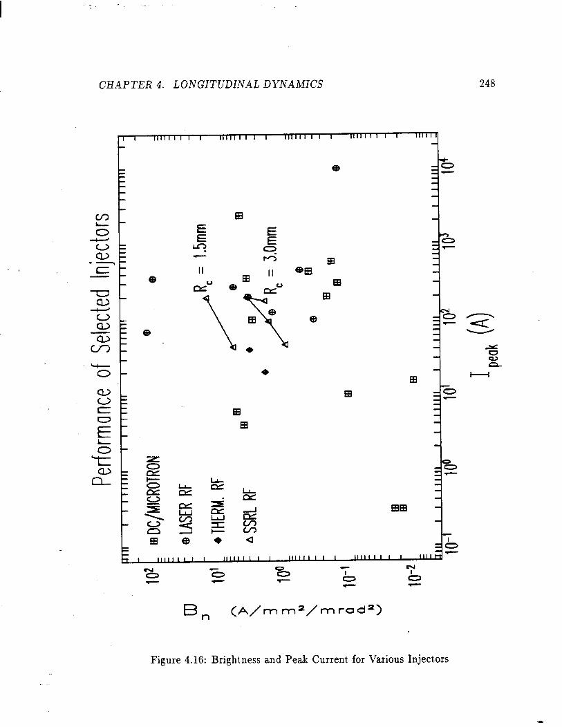
-
CHAPTER 4. LONGITUDINAL DYNAMICS
I’ ’ lllllII I I lllllII I I llllI I I I I lllllII I l llll I q
t
E q
0
e
e
q
q
248
B* (A/mm2/mrad2)
Figure 4.16: Bright.ness and Peak Current, for Various Inject,ors

.
CH.4PTER 4. LONGITUDINAL DI’NAMICS 249
Table 4.6: Performance of RF-Gun-Based Injectors
Project, G I peak Q St %I t,ype
7r-m,c-pm A nC ps A/mm2/mr2
ANL[14] 340 10 - lo3 100 8 0.17 laser
CERN[14] 3i.5 450 9 30 0.64 laser
_- LANL: - AFEL[14] 2.5 350 5 16 112 laser
HIBAFjl4] 9.0 270 4 15 6.7 laser
PHASE I[ 141 10.0 200 11 70 4.0 laser
SSRL: 3nun,40A/cn~2 9.5 196 0.2 1.0 4.4 t,herm.
1.5rnrn,80A/cm2 4.8 144 0.2 0.7 lf.2 t,herm.