chapter 4. discrete probability...

Discrete Probability Distributions - 57

Chapter 4. Discrete Probability Distributions

4.1. Introduction

In Chapter 2, we learned how to compute probabilities and cumulative probabilities for arbitrary discrete and continuous probability distribution functions (PDFs). In Chapter 3, we learned how to compute expectations, such as the mean and variance, of random variables and functions of them, given a PDF, f(x). In this chapter, we introduce some of the commonly occurring PDFs for discrete sample spaces. We will apply the rules of Chapters 2 and 3, to use the PDFs to calculate probabilities and expectations. The goal of this section is to become familiar with these probability distributions and, when given a problem, know which PDF is appropriate.

4.2. Discrete Uniform Distribution

If the random variable X assumes the values of x1, x2, x3… xk with equal probability, then the discrete uniform distribution is given by f(x;k) (The semicolon is used to separate random variables, which shall always appear before the semicolon, from parameters, which appear after.)

kkxf 1);( = (4.1)

In calculating the mean and variance of the Discrete Uniform Distribution PDF, or any discrete PDF for that matter, we have a definition given in equation (3.1.a), namely

∑==

xx xxfxE )()(µ (3.1.a)

Using this formula will always give the correct result. However, if the number of elements in

the sample space is infinite, it will not be practical to explicitly evaluate each term in the summation. For many of these commonly occurring PDFs, the evaluation of the definition of the mean reduces to a formula for the mean. In some cases, the formula is easy to derive and in other cases, more difficult. Some PDFs have no simple expression for the mean or variance.

For the Discrete Uniform Distribution, the PDF is a constant. Consequently, the mean of the random variable, x, is given by


∑=

=k

iix x

k 1

1µ (4.2)

The variance of the random variable, x, obeying the Discrete Uniform Distribution is given by

( )2

1

2 1 ∑=

−=k

ixix x

kµσ (4.3)

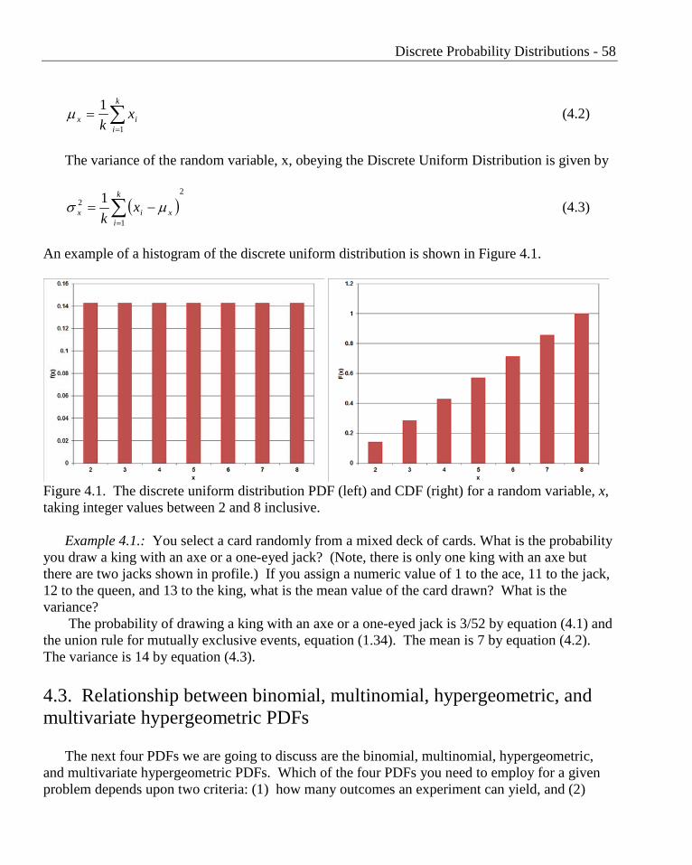
An example of a histogram of the discrete uniform distribution is shown in Figure 4.1.

Figure 4.1. The discrete uniform distribution PDF (left) and CDF (right) for a random variable, x, taking integer values between 2 and 8 inclusive.

Example 4.1.: You select a card randomly from a mixed deck of cards. What is the probability you draw a king with an axe or a one-eyed jack? (Note, there is only one king with an axe but there are two jacks shown in profile.) If you assign a numeric value of 1 to the ace, 11 to the jack, 12 to the queen, and 13 to the king, what is the mean value of the card drawn? What is the variance?

The probability of drawing a king with an axe or a one-eyed jack is 3/52 by equation (4.1) and the union rule for mutually exclusive events, equation (1.34). The mean is 7 by equation (4.2). The variance is 14 by equation (4.3).

4.3. Relationship between binomial, multinomial, hypergeometric, and multivariate hypergeometric PDFs

The next four PDFs we are going to discuss are the binomial, multinomial, hypergeometric, and multivariate hypergeometric PDFs. Which of the four PDFs you need to employ for a given problem depends upon two criteria: (1) how many outcomes an experiment can yield, and (2)


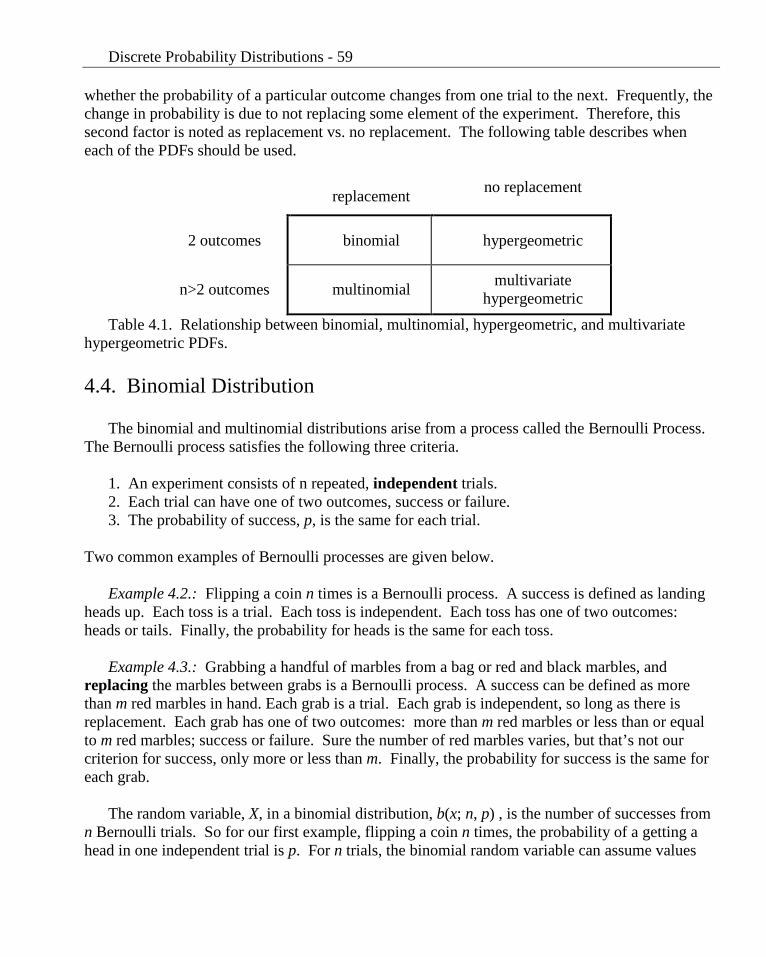
whether the probability of a particular outcome changes from one trial to the next. Frequently, the change in probability is due to not replacing some element of the experiment. Therefore, this second factor is noted as replacement vs. no replacement. The following table describes when each of the PDFs should be used.

replacement no replacement

2 outcomes binomial hypergeometric

n>2 outcomes multinomial multivariate hypergeometric

Table 4.1. Relationship between binomial, multinomial, hypergeometric, and multivariate hypergeometric PDFs.

4.4. Binomial Distribution

The binomial and multinomial distributions arise from a process called the Bernoulli Process. The Bernoulli process satisfies the following three criteria.

1. An experiment consists of n repeated, independent trials. 2. Each trial can have one of two outcomes, success or failure. 3. The probability of success, p, is the same for each trial.

Two common examples of Bernoulli processes are given below.

Example 4.2.: Flipping a coin n times is a Bernoulli process. A success is defined as landing heads up. Each toss is a trial. Each toss is independent. Each toss has one of two outcomes: heads or tails. Finally, the probability for heads is the same for each toss.

Example 4.3.: Grabbing a handful of marbles from a bag or red and black marbles, and

replacing the marbles between grabs is a Bernoulli process. A success can be defined as more than m red marbles in hand. Each grab is a trial. Each grab is independent, so long as there is replacement. Each grab has one of two outcomes: more than m red marbles or less than or equal to m red marbles; success or failure. Sure the number of red marbles varies, but that’s not our criterion for success, only more or less than m. Finally, the probability for success is the same for each grab.

The random variable, X, in a binomial distribution, b(x; n, p) , is the number of successes from

n Bernoulli trials. So for our first example, flipping a coin n times, the probability of a getting a head in one independent trial is p. For n trials, the binomial random variable can assume values


between 0 (never getting a head) up to n (getting a head every time). The distribution gives the probability for getting a particular value of successes in n trials.

The binomial distribution is (where q the probability of a failure is q = 1 - p)

xnxqpxn

pnxbxXP −

=== ),;()( (4.4)

Without derivation, the mean of the random variable, x, obeying the binomial PDF is

npx =µ (4.5) The variance of the random variable, x, obeying the the binomial PDF is

npqx =2σ (4.6) Frequently, we are interested in the cumulative PDF, as defined in equation (2.X).

( )∑≤

=

=≤rx

ii

i

xfrXP1

)( (2.X)

The cumulative probability distribution of the binomial PDF is obtained by substituting the

binomial PDF in equation (4.) into the equation above,

∑=

=≡≤r

xpnxbpnrBrXP

0),;(),;()( (4.7)

There are a variety of ways to calculate the cumulative binomial PDF for given values of r, n

and p. In the old days, when cavemen wanted to calculate cumulative probabilities based on the binomial distribution, they turned to tables of values chiseled on the stone walls of their caves. In later years, these tables were transcribed into the appendices of statistics textbooks. Yet later, these same tables were transcribed onto files available on the internet, where a cursory search of “cumulative binomial distribution tables” will turn up numerous examples.

The disadvantage of using tables, aside from the fact that many of us may find the comparison to cavemen to be an unflattering one, is that the parameter, p, can take on any value between 0 and 1, but the tables only provide values of the cumulative PDF for a few values of p, usually, 0.1, 0.2...0.8, 0.9. For any other value of p, we must interpolate in the table, which adds an unnecessary error.

We can also use modern computational tools to evaluate the binomial PDF and the cumulative binomial PDF (the binomial CDF) for any arbitrary values of r, n and p. What follows are two paths to computing the PDF and CDF for the binomial distribution. In the first path, we write our own little codes. This exercise is instructive because it illustrates the simplicity of the process. In


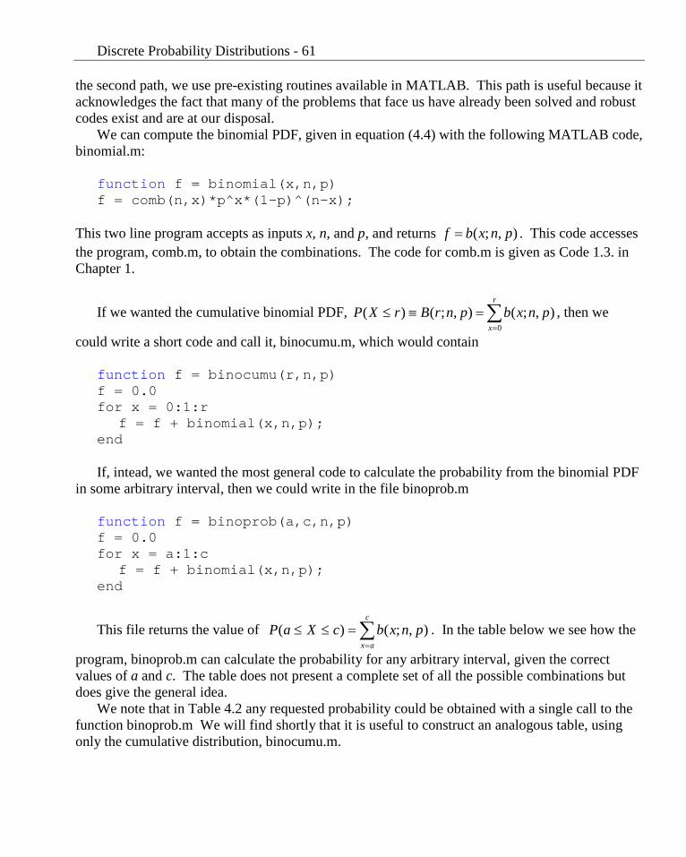
the second path, we use pre-existing routines available in MATLAB. This path is useful because it acknowledges the fact that many of the problems that face us have already been solved and robust codes exist and are at our disposal.

We can compute the binomial PDF, given in equation (4.4) with the following MATLAB code, binomial.m:

function f = binomial(x,n,p) f = comb(n,x)*p^x*(1-p)^(n-x);

This two line program accepts as inputs x, n, and p, and returns ),;( pnxbf = . This code accesses the program, comb.m, to obtain the combinations. The code for comb.m is given as Code 1.3. in Chapter 1.

If we wanted the cumulative binomial PDF, ∑=

=≡≤r

xpnxbpnrBrXP

0),;(),;()( , then we

could write a short code and call it, binocumu.m, which would contain function f = binocumu(r,n,p) f = 0.0 for x = 0:1:r

f = f + binomial(x,n,p); end If, intead, we wanted the most general code to calculate the probability from the binomial PDF

in some arbitrary interval, then we could write in the file binoprob.m function f = binoprob(a,c,n,p) f = 0.0 for x = a:1:c

f = f + binomial(x,n,p); end

This file returns the value of ∑=

=≤≤c

axpnxbcXaP ),;()( . In the table below we see how the

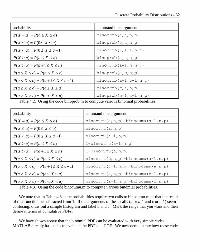
program, binoprob.m can calculate the probability for any arbitrary interval, given the correct values of a and c. The table does not present a complete set of all the possible combinations but does give the general idea.

We note that in Table 4.2 any requested probability could be obtained with a single call to the function binoprob.m We will find shortly that it is useful to construct an analogous table, using only the cumulative distribution, binocumu.m.


probability command line argument

)()( aXaPaXP ≤≤== binoprob(a,a,n,p)

)0()( aXPaXP ≤≤=≤ binoprob(0,a,n,p)

)10()( −≤≤=< aXPaXP binoprob(0,a-1,n,p)

)()( nXaPaXP ≤≤=≥ binoprob(a,n,n,p)

)1()( nXaPaXP ≤≤+=> binoprob(a+1,n,n,p)

)()( cXaPcXaP ≤≤=≤≤ binoprob(a,c,n,p)

)11()( −≤≤+=<< cXaPcXaP binoprob(a+1,c-l,n,p)

)()( aXcPcXaP ≤≤=≥≥ binoprob(c,a,n,p)

)()( aXcPcXaP <<=>> binoprob(c+1,a-l,n,p) Table 4.2. Using the code binoprob.m to compute various binomial probabilities.

probability command line argument

)()( aXaPaXP ≤≤== binocumu(a,n,p)-binocumu(a-1,n,p)

)0()( aXPaXP ≤≤=≤ binocumu(a,n,p)

)10()( −≤≤=< aXPaXP binocumu(a-1,n,p)

)()( nXaPaXP ≤≤=≥ 1-binocumu(a-1,n,p)

)1()( nXaPaXP ≤≤+=> 1-binocumu(a,n,p)

)()( cXaPcXaP ≤≤=≤≤ binocumu(c,n,p)-binocumu(a-1,n,p)

)11()( −≤≤+=<< cXaPcXaP binocumu(c-1,n,p)-binocumu(a,n,p)

)()( aXcPcXaP ≤≤=≥≥ binocumu(a,n,p)-binocumu(c-1,n,p)

)()( aXcPcXaP <<=>> binocumu(a-1,n,p)-binocumu(c,n,p) Table 4.3. Using the code binocumu.m to compute various binomial probabilities. We note that in Table 4.3 some probabilities require two calls to binocumu.m or that the result

of that function be subtracted from 1. If the arguments of these calls (a or a-1 and c or c-1) seem confusing, draw out a sample histogram and label a and c. Mark the range that you want and then define it terms of cumulative PDFs.

We have shown above that the binomial PDF can be evaluated with very simple codes.

MATLAB already has codes to evaluate the PDF and CDF. We now demonstrate how these codes


can be used. A summary of these MATLAB commands is given in Appendix IV. In order to evaluate a PDF at a given value of x, one can use the pdf function in MATLAB

>> f = pdf('Binomial',x,n,p) For example, to generate the value of the PDF for the binomial PDF defined for x = 1, n = 4

and p = 0.33, one can type the command, >> f = pdf('Binomial',1,4,0.33) which yields the following output (when the format long command has first been used to

provide all sixteen digits) f = 0.397007160000000 This tells us that the probability of getting 1 success in four attempts where the probability of

success of an individual is given by 0.33 is about 0.397. In order to evaluate a cumulative PDF or CDF at a given value of x, one can use the cdf

function in MATLAB. If we are interested in the probability that rx ≤ , then the appropriate function is the cumulative distribution function.

( ) ( )∑=

≡≤=r

xpnxbrxpF

0,;

In MATLAB, we can directly evaluate the cumulative distribution function for a number of common PDFs.

>> F = cdf('Binomial',x,n,p) For example, to generate the value of the binomial CDF for x ≤ 1, n = 4 and p = 0.33, one can

type the command, >> F = cdf('Binomial',1,4,0.33) which yields the following output F = 0.598518370000000

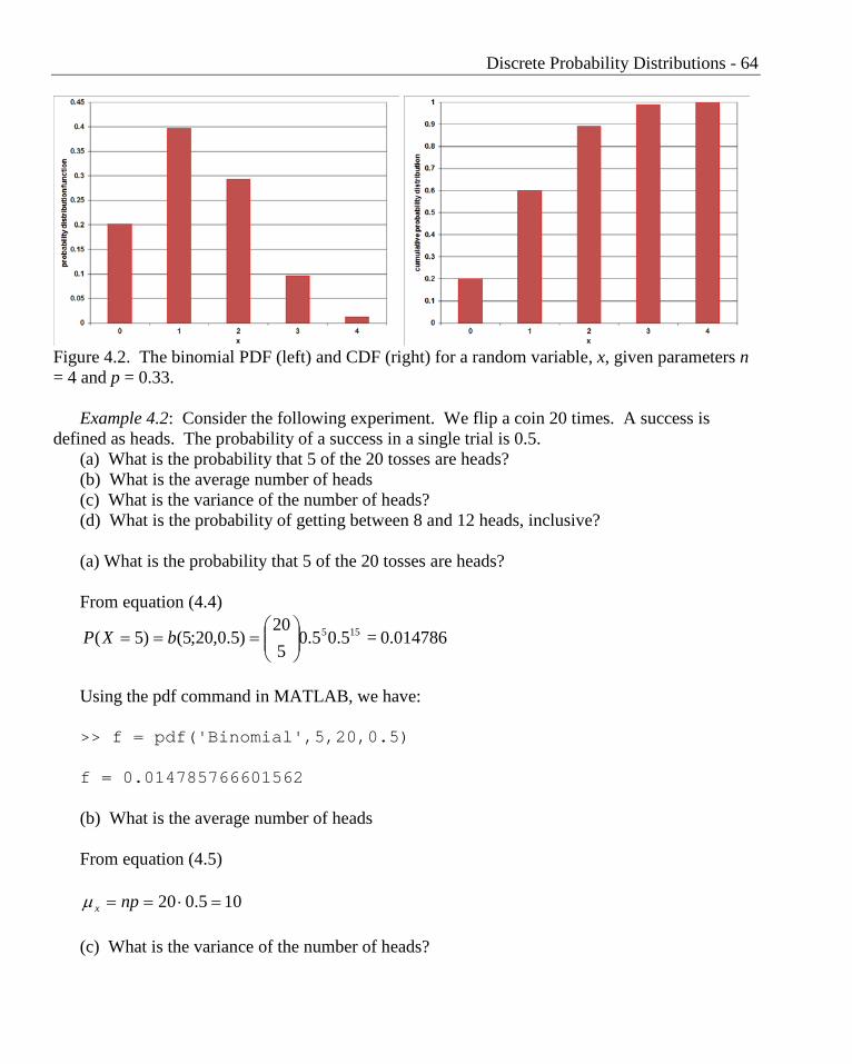
An example of a histogram of the binomial distribution is shown in Figure 4.2.


Figure 4.2. The binomial PDF (left) and CDF (right) for a random variable, x, given parameters n = 4 and p = 0.33.

Example 4.2: Consider the following experiment. We flip a coin 20 times. A success is defined as heads. The probability of a success in a single trial is 0.5.

(a) What is the probability that 5 of the 20 tosses are heads? (b) What is the average number of heads (c) What is the variance of the number of heads? (d) What is the probability of getting between 8 and 12 heads, inclusive? (a) What is the probability that 5 of the 20 tosses are heads? From equation (4.4)

0.014786 =5.05.0520

)5.0,20;5()5( 155

=== bXP

Using the pdf command in MATLAB, we have: >> f = pdf('Binomial',5,20,0.5) f = 0.014785766601562 (b) What is the average number of heads From equation (4.5)

105.020 =⋅== npxµ (c) What is the variance of the number of heads?

Discrete Probability Distributions - 65 From equation (4.6)

55.05.0202 =⋅⋅== npqxσ (d) What is the probability of getting between 8 and 12 heads, inclusive? If we rely on the cumulative distribution function, we can write this probability as

)8()12()128( <−≤=≤≤ XPXPXP

)7()12()128( ≤−≤=≤≤ XPXPXP

)5.0,20;7()5.0,20;12()128( ===−====≤≤ pnrBpnrBXP We can use a table from the web and obtain

7368.01316.08684.0)128( =−=≤≤ XP We can use the cdf function in MATLAB >> p = cdf('Binomial',12,20,0.5) - cdf('Binomial',7,20,0.5)

F = 0.736824035644531 So when you give a coin 20 flips, roughly 74% of the time, you will wind up with between 8

and 12 heads, inclusive. Does this mean 30% of the time you will wind up with 8 to 12 tails, inclusive? Why or why not?

4.5. Multinomial Distribution

If a Bernoulli trial can have more than 2 outcomes (success or failure) then it ceases to be a Bernoulli trial and becomes a multinomial experiment. In the multinomial experiment, there are k outcomes and n trials. Each outcome has a result Ei. There are now k random variables Xi, each representing the probability of obtaining result Ei in Xi of the n trials.

The distribution of a multinomial experiment is

∏=

===

k

i

x

k

i

ip

xxxn

kpnxmxXP121 ...,

),,;()( (4.8)


where ∑=

=k

ii nx

1

and ∑=

=k

iip

11.

Note that in order to evaluate the multinomial PDF, we require two vectors. A vector of probabilities for each outcome, p , and a vector of the number of each outcome that we are interested in, x . We can again use modern computational tools to evaluate the multinomial PDF for any arbitrary values of x , n, p and k. What follows are two paths to computing the PDF for the multinomial distribution. In the first path, we write our own little code. This exercise is instructive because it illustrates the simplicity of the process. In the second path, we use a pre-existing routine available in MATLAB.

First, we can write a code to evaluate ),,;()( kpnxmxXP == , such as the one in multinomial.m

function prob = multinomial(x,n,p,k) prob = factorial(n); for i = 1:1:k prob = prob/factorial(x(i))*p(i)^x(i); end In the code, multinomial.m, x and p are vectors of length k. This code would be run at the

command prompt with something like >> f = multinomial([2,4,3],9,[0.5,0.3,0.2],3)

where ]3,4,2[=x , n = 9, ]2.0,3.0,5.0[=p and k = 3. This command yields

f = 0.020412000000000 Alternatively, there is an intrinsic function in MATLAB, but it is not the usual pdf function. For the multinomial distribution, there is a special command, mnpdf.

>> f = mnpdf(x,p) In this case, we didn’t have to input the parameters n and k because the code knows that the sum of the elements in the vector x is n and the number of elements in the vector x is k. An example of the use of this function, where ]3,4,2[=x , n = 9, ]2.0,3.0,5.0[=p and k = 3, is

>> f = mnpdf([2,4,3],[0.5,0.3,0.2]) This command yields


f = 0.020412000000000 There are not any intrinsic routines for computing probabilities over ranges of variables for the multinomial distribution. Simple codes could be written following the model of binoprob.m.

Example 4.3.: A hypothetical statistical analysis of people moving to Knoxville, TN shows that 25% of people who move here do so to attend the University, 55% move here for a professional position, and the remaining 20% for some other reason. If you ask 10 new arrivals in Knoxville, why they moved here, what is the probability that all of them moved here to go to UT?

In this problem, there are ten new arrivals. Each is considered an experiment, thus n = 10.

There are three possible outcomes: U=university, P=profession and O=other, thus k = 3. The probabilities of each outcome are 25.0=Up , 55.0=Pp and 20.0=Op . In this question we are asked to find the probability that 10=Ux , 0=Px and 0=Ox .

Using equation (4.7), we have

{ } 007-9.54e20.055.025.0!0!0!10

!10)3],20.0,55.0,25.0[,10];0,0,10([])0,0,10[( 0010 ==== mXP

Using the mnpdf function in MATLAB, we can accomplish the same task. >> f = mnpdf([10,0,0],[0.25,0.55,0.2]) f =

9.536743164062500e-07

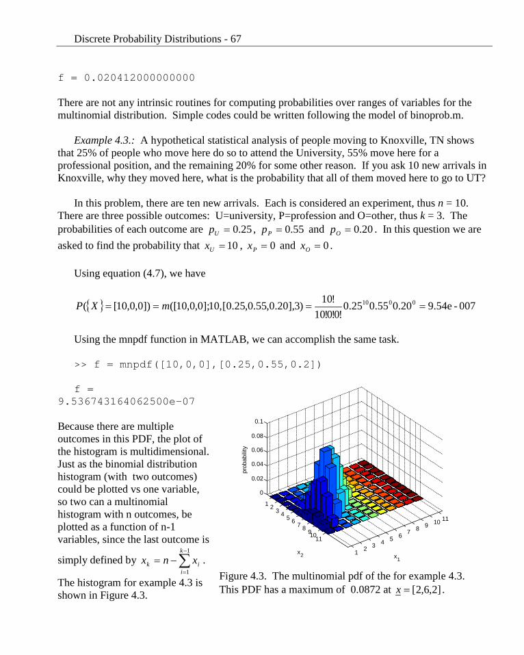
Because there are multiple outcomes in this PDF, the plot of the histogram is multidimensional. Just as the binomial distribution histogram (with two outcomes) could be plotted vs one variable, so two can a multinomial histogram with n outcomes, be plotted as a function of n-1 variables, since the last outcome is

simply defined by ∑−

=

−=1

1

k

iik xnx .

The histogram for example 4.3 is shown in Figure 4.3.

Figure 4.3. The multinomial pdf of the for example 4.3. This PDF has a maximum of 0.0872 at ]2,6,2[=x .

1 2 3 4 5 6 7 8 9 10 11

1 2 3 4 5 6 7 8 91011

0

0.02

0.04

0.06

0.08

0.1

x1x2

prob

abili

ty


4.6. Hypergeometric Distribution

The hypergeometric distribution applies when 1. A random sample of size n is selected without replacement from a sample space

containing N total items. 2. k of the N items may be classified as successes and N-k are classified as failures.

(Therefore, there are only I outcomes in the experiment.)

The hypergeometric distribution differs from the binomial distribution because the probability of success changes with each trial during the course of the experiment in the hypergeometric case. By contrast, p is constant in the binomial case.

The probability distribution of the hypergeometric random variable X, the number of successes

in a random sample of size n selected from a sample space containing a total of N items, in which k of N are will be labeled as a success and N - k will be labeled failure is

...n,,x

nN

xnkN

xk

knNxh 210for ),,;( =

−−

= (4.9)

The mean of a random variable that follows the hypergeometric distribution h(x;N,n,k) is

Nnk

x =µ (4.10)

and the variance of a random variable that follows the hypergeometric distribution

−

−−

=Nk

Nnk

NnN

x 11

2σ (4.11)

Example 4.5: What is the probability of getting dealt 4 of a kind in a hand of five-card-

stud poker? We can use the hypergeometric distribution on this problem because we are going to select

n=5 from N=52. We don’t care about what value of the cards the four of a kind is in so we can just calculate the result for aces and then multiply that probability by 13 since there are 13 values of cards and a four of a kind of any of them are equally likely. Therefore, a success is an ace and a failure is not an ace. k = 4 aces. For a four of kind x = 4 aces.


541451

552

148

44

552

45452

44

)4,5,52;4( =

=

−−

=h

We multiply that by 13 to get the probability of a four-of-a-kind as being: 0.00024. Or, one out of every 4165 hands dealt is probably a four of a kind.

We can also use modern computational tools to evaluate the hypergeometric PDF and CDF.

Again, we first show a simple code for the PDF, then demonstrate the use of the intrinsic MATLAB functions.

We can compute the hypergeometric PDF, ),,;()( knNxhxXP == , given in equation (4.9) with the following MATLAB code, hypergeo.m:

function prob = hypergeo(x,ntot,nsamp,k) denom = comb(ntot,nsamp); numerator = comb(k,x)*comb(ntot-k,nsamp-x); prob = numerator/denom; As an example, if we want to know what is the probability that we draw 3 red marbles in four

attempts from a bag containing 5 red marbles and 6 green marbles, then we have x=3, n=4, k=5 and N=5+6=11.

>> f = hypergeo(3,11,4,5)

which returns a value

f = 0.181818181818182

We can also use the pdf function in MATLAB

>> f = pdf('Hypergeometric',x,N,k,n) For example, to generate the value of the hypergeometric PDF defined for x=3, n=4, k=5 and

N=11, one can type the command, >> f = pdf('Hypergeometric',3,11,5,4) which yields the following output f = 0.181818181818182

Discrete Probability Distributions - 70 This tells us that the probability of getting 3 red marbles when drawing 4 marbles from a bag

initially containing 11 total marbles, 5 of which are red, is about 0.182. In order to evaluate a cumulative PDF or CDF at a given value of x, one can use the cdf

function in MATLAB. If we are interested in the probability that rx ≤ , then the appropriate function is the cumulative distribution function, cdf.

( ) ∑=

≡≤=r

xknNxhrxpF

0),,;(

>> F = cdf('Hypergeometric',x,N,k,n) For example, to generate the value of the binomial CDF for x ≤ 3, n=4, k=5 and N=11, one can

type the command, >> f = cdf('Hypergeometric',3,11,5,4) which yields the following output f = 0.984848484848485

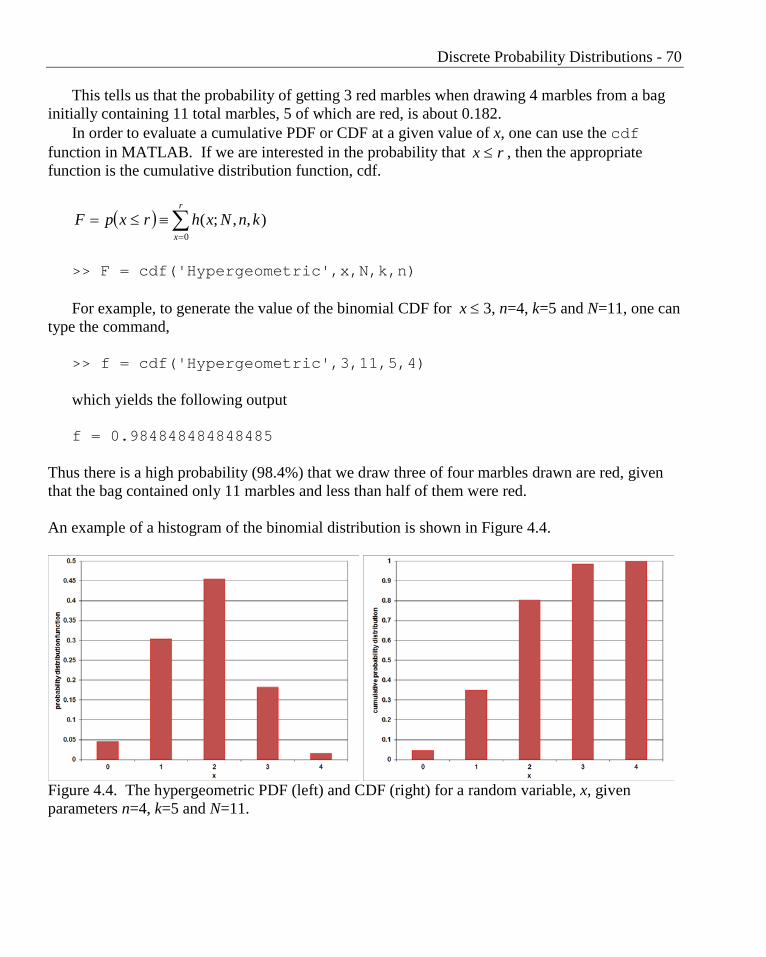
Thus there is a high probability (98.4%) that we draw three of four marbles drawn are red, given that the bag contained only 11 marbles and less than half of them were red. An example of a histogram of the binomial distribution is shown in Figure 4.4.

Figure 4.4. The hypergeometric PDF (left) and CDF (right) for a random variable, x, given parameters n=4, k=5 and N=11.


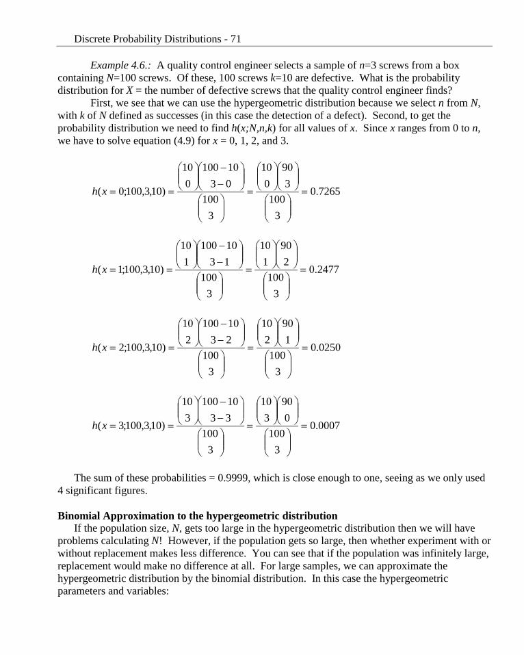
Example 4.6.: A quality control engineer selects a sample of n=3 screws from a box containing N=100 screws. Of these, 100 screws k=10 are defective. What is the probability distribution for X = the number of defective screws that the quality control engineer finds?

First, we see that we can use the hypergeometric distribution because we select n from N, with k of N defined as successes (in this case the detection of a defect). Second, to get the probability distribution we need to find h(x;N,n,k) for all values of x. Since x ranges from 0 to n, we have to solve equation (4.9) for x = 0, 1, 2, and 3.

7265.0

3100

390

010

3100

0310100

010

)10,3,100;0( =

=

−−

==xh

2477.0

3100

290

110

3100

1310100

110

)10,3,100;1( =

=

−−

==xh

0250.0

3100

190

210

3100

2310100

210

)10,3,100;2( =

=

−−

==xh

0007.0

3100

090

310

3100

3310100

310

)10,3,100;3( =

=

−−

==xh

The sum of these probabilities = 0.9999, which is close enough to one, seeing as we only used

4 significant figures.

Binomial Approximation to the hypergeometric distribution If the population size, N, gets too large in the hypergeometric distribution then we will have

problems calculating N! However, if the population gets so large, then whether experiment with or without replacement makes less difference. You can see that if the population was infinitely large, replacement would make no difference at all. For large samples, we can approximate the hypergeometric distribution by the binomial distribution. In this case the hypergeometric parameters and variables:


),;(),,;(NkpnxbknNxh =≈

where we see that probability, p, is estimated as the fraction of the N elements that are defined as success.

4.7. Multivariate Hypergeometric Distribution

Just as the binomial distribution can be adjusted to account for multiple random variables (i.e. the multinomial distribution) so too can the hypergeometric distribution account for multiple random variables (multivariate hypergeometric distribution). The multivariate hypergeometric distribution is defined as

...

),,,;( 3

3

2

2

1

1

=

nN

xa

xa

xa

xa

kanNxh k

k

m (4.12)

where xi is the number of outcomes of the ith result in n trials and ai is the number of objects of the ith type in the total population of N, and k is the number of types of outcomes. Clearly, the following constraints apply. The total number of each outcome must equal the number of trials,

namely ∑=

=k

ii nx

1

. The total number of objects must equal the total population, ∑=

=k

ii Na

1

.

We can use modern computational tools to evaluate the multivariate hypergeometric distribution. We can write a code to evaluate { } ),,,;()( kanNxhxXP m== , such as the one in multihypergeo.m

function prob = multihypergeo(x,ntot,nsamp,a,k) denom = comb(ntot,nsamp); numerator = 1.0; for i = 1:1:k numerator = numerator*comb(a(i),x(i)); end prob = numerator/denom; In the code, multihypergeo.m, x and a are vectors of length k. As an example, if we want to

know what is the probability that we draw 3 red marbles and 1 green marble in 4 attempts from a bag containing 5 red marbles and 6 green marbles and 2 blue marbles, then we have ]0,1,3[=x , N=5+6+2=13, n=4, ]2,6,5[=a and k=3.

Discrete Probability Distributions - 73 >> f = multihypergeo([3,1,0],13,4,[5,6,2],3)

which returns a value f = 0.083916083916084 MATLAB doesn’t have an intrinsic function for the multivariate hypergeometric distribution. Example 4.7.: A unethical vendor has some defective computer merchandise that he is trying

to unload. He has 24 computers. Of these, 12 are ok, 4 others have bad motherboards, 2 others have bad video cards, and 8 others have bad sound cards. If we go into buy 5 computers from this vendor, what is the probability we get 3 good computers, 1 with a bad sound card and 1 with a bad video card?

In this problem, we have ]1,1,0,3[=x , N=24, n=5, ]8,2,4,12[=a and k=4.

{ } 0.08282

524

18

12

04

312

)],8,2,4,12[,5,24];1,1,0,3([])1,1,0,3[( =

=== khXP m

So there is about an 8.2% chance that when we purchase five computers from this vendor that we get 3 good computers, 1 with a bad sound card and 1 with a bad video card.

4.8. Negative Binomial Distribution

Like the binomial distribution, the negative binomial distribution applies to a Bernoulli process, but it asks a different question. As a reminder the Bernoulli process satisfies the following three criteria:

1. An experiment that consists of x repeated, independent trials. 2. Each trial can have one of two outcomes, success or failure. 3. The probability of success, p, is the same for each trial. The negative binomial distribution applies when a fourth criteria is added. 4. The trials are continued until we achieve the kth success. This is the Bernoulli process, except that in the binomial distribution, we fixed n trials and

allowed x, the number of successes to be the random variable. In the negative binomial


distribution, we fix k successes and allow the number of trials, now labelled x, to be the random variable.

The probability distribution of the negative binomial random variable X, the number of trials needed to obtain k successes is

.2111

..,kk,k for xqpkx

(x;k,p)b x-kk* ++=

−−

= (4.13)

Remember the probability of failure is one less the probability of success, q = 1-p.

We can also use modern computational tools to evaluate the negative binomial PDF and CDF. Again, we first show a simple code for the PDF, then demonstrate the use of the intrinsic MATLAB functions.

We can compute the negative binomial PDF, ),;()( * pkxbxXP == , given in equation (4.13) with the following MATLAB code, negbinomial.m:

function prob = negbinomial(x,k,p) prob = comb(x-1,k-1)*p^k*(1-p)^(x-k); As an example, if we want to know what is the probability that we draw flip our second head

on our fourth trial, where p=0.5, we have x=4 and k=2 >> f = negbinomial(4,2,0.5)


f = 0.187500000000000


>> f = pdf('Negative Binomial',x-k,k,p) This formulation with the random variable being x-k, rather than x is due to alternate

formulations of the negative binomial distribution, in which the function assumes the random variable is the number of failures, not the number of trials. The number of failures is the number of trials less the number of successes. For example, to generate the value of the negative binomial PDF defined for x=4, k=2 and p=0.5, one can type the command,

>> f = pdf('Negative Binomial',4-2,2,0.5) which yields the following output f = 0.187500000000000

Discrete Probability Distributions - 75 In order to evaluate a cumulative PDF or CDF at a given value of x, one can use the cdf


( ) ∑=

≡≤=r

kxpkxbrxpF ),;(*

>> F = cdf('Negative Binomial',x-k,k,p) For example, to generate the value of the negative binomial PDF defined for x ≤ 4, k=2 and

p=0.5, one can type the command, >> F = cdf('Negative Binomial',4-2,2,0.5) which yields the following output F = 0.687500000000000

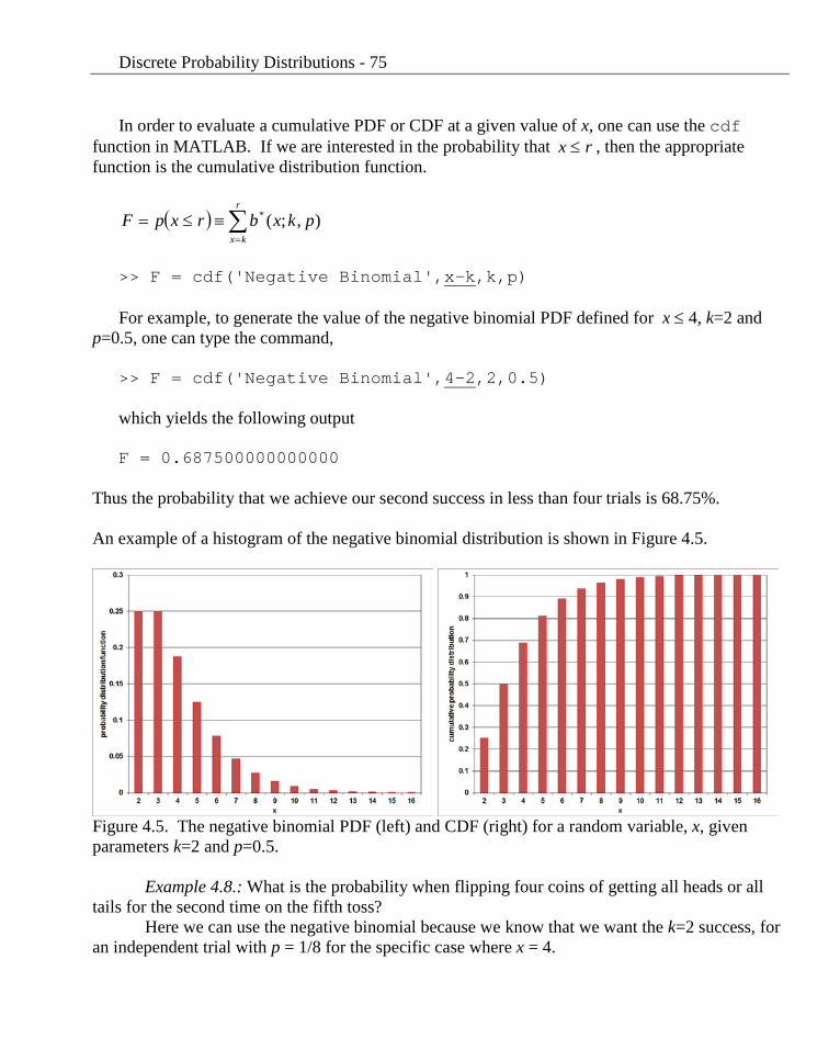
Thus the probability that we achieve our second success in less than four trials is 68.75%. An example of a histogram of the negative binomial distribution is shown in Figure 4.5.

Figure 4.5. The negative binomial PDF (left) and CDF (right) for a random variable, x, given parameters k=2 and p=0.5.

Example 4.8.: What is the probability when flipping four coins of getting all heads or all tails for the second time on the fifth toss?

Here we can use the negative binomial because we know that we want the k=2 success, for an independent trial with p = 1/8 for the specific case where x = 4.


0.0418787

81

1215

)8/1,2;5(32

* =

−−

=b

>> f = pdf('Negative Binomial',5-2,2,1/8) which yields the following output f = 0.041870117187500 So there is 4.2% chance when flipping four coins of getting all heads or all tails for the second

time on the fifth trial.

4.9. Geometric Distribution

The geometric distribution is a subset of the negative binomial distribution when k=1. That is, the geometric distribution gives the probability that the first success occurs on the random variable X, the number of the trial. This corresponds to a system where the Bernoulli process stops after the first success. If success is defined as a “failure” of the system, a crash of a code, or an explosion, or some fault in the process, which causes the system to stop functioning, then in this case, we are only interested in one such success, so k=1 and we have the geometric distribution.

The probability distribution of the geometric random variable X, the number of trials needed to obtain the first success is

.321for 1 ..,,xpqg(x;p) x- == (4.14)

The mean of a random variable following the geometric distribution is

px1

=µ (4.15)

and the variance is

22 1

pp

x−

=σ (4.16)

Remember the probability of failure is one less the probability of success, q = 1-p.

We can also use modern computational tools to evaluate the geometric PDF and CDF. Again, we first show a simple code for the PDF, then demonstrate the use of the intrinsic MATLAB functions.

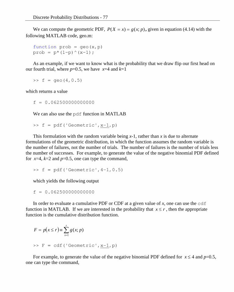
Discrete Probability Distributions - 77 We can compute the geometric PDF, );()( pxgxXP == , given in equation (4.14) with the

following MATLAB code, geo.m: function prob = geo(x,p) prob = p*(1-p)^(x-1); As an example, if we want to know what is the probability that we draw flip our first head on

our fourth trial, where p=0.5, we have x=4 and k=1 >> f = geo(4,0.5)


f = 0.062500000000000


>> f = pdf('Geometric',x-1,p) This formulation with the random variable being x-1, rather than x is due to alternate

formulations of the geometric distribution, in which the function assumes the random variable is the number of failures, not the number of trials. The number of failures is the number of trials less the number of successes. For example, to generate the value of the negative binomial PDF defined for x=4, k=2 and p=0.5, one can type the command,

>> f = pdf('Geometric',4-1,0.5) which yields the following output f = 0.062500000000000 In order to evaluate a cumulative PDF or CDF at a given value of x, one can use the cdf


( ) ∑=

≡≤=r

xpxgrxpF

1);(

>> F = cdf('Geometric',x-1,p) For example, to generate the value of the negative binomial PDF defined for x ≤ 4 and p=0.5,

one can type the command,

Discrete Probability Distributions - 78 >> F = cdf('Geometric',4-1,0.5)

which yields the following output F = 0.937500000000000

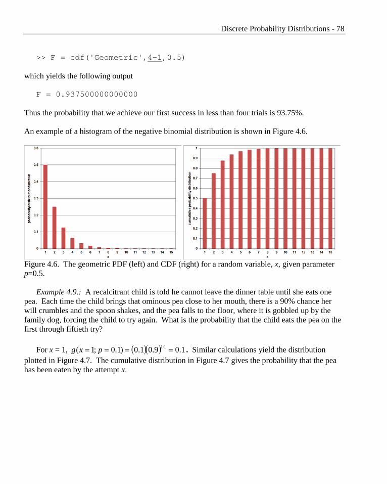
Thus the probability that we achieve our first success in less than four trials is 93.75%. An example of a histogram of the negative binomial distribution is shown in Figure 4.6.

Figure 4.6. The geometric PDF (left) and CDF (right) for a random variable, x, given parameter p=0.5.

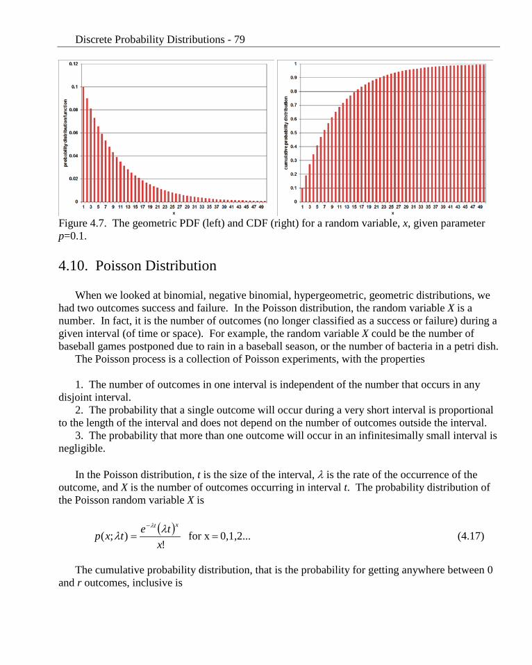
Example 4.9.: A recalcitrant child is told he cannot leave the dinner table until she eats one pea. Each time the child brings that ominous pea close to her mouth, there is a 90% chance her will crumbles and the spoon shakes, and the pea falls to the floor, where it is gobbled up by the family dog, forcing the child to try again. What is the probability that the child eats the pea on the first through fiftieth try?

For x = 1, ( )( ) 0.10.91.0)1.0;1( 1-1 ==== pxg . Similar calculations yield the distribution

plotted in Figure 4.7. The cumulative distribution in Figure 4.7 gives the probability that the pea has been eaten by the attempt x.


Figure 4.7. The geometric PDF (left) and CDF (right) for a random variable, x, given parameter p=0.1.

4.10. Poisson Distribution

When we looked at binomial, negative binomial, hypergeometric, geometric distributions, we had two outcomes success and failure. In the Poisson distribution, the random variable X is a number. In fact, it is the number of outcomes (no longer classified as a success or failure) during a given interval (of time or space). For example, the random variable X could be the number of baseball games postponed due to rain in a baseball season, or the number of bacteria in a petri dish.

The Poisson process is a collection of Poisson experiments, with the properties 1. The number of outcomes in one interval is independent of the number that occurs in any

disjoint interval. 2. The probability that a single outcome will occur during a very short interval is proportional

to the length of the interval and does not depend on the number of outcomes outside the interval. 3. The probability that more than one outcome will occur in an infinitesimally small interval is

negligible. In the Poisson distribution, t is the size of the interval, λ is the rate of the occurrence of the

outcome, and X is the number of outcomes occurring in interval t. The probability distribution of the Poisson random variable X is

( ) 0,1,2... for x !

);( ==−

xtetxp

xt λλλ

(4.17)

The cumulative probability distribution, that is the probability for getting anywhere between 0

and r outcomes, inclusive is


∑=

=r

xtxptrP

0);();( λλ (4.18)

The mean and the variance of the Poisson distribution are

txx λσµ == 2 (4.19) The Poisson distribution is the asymptotical form of the binomial distribution when n, the

number of trials, goes to infinity, p, the probability of a success goes to zero, and the mean (np) remains constant. We do not prove this relation here.

We can also use modern computational tools to evaluate the geometric PDF and CDF. Again, we first show a simple code for the PDF, then demonstrate the use of the intrinsic MATLAB functions.

We can compute the Poisson PDF, );()( txpxXP λ== , given in equation (4.17) with the following MATLAB code, poisson.m:

function f = poisson(x,p) f= exp(-p)*p^x/factorial(x);

As an example, if we want to know what is the probability that we observe x = 2 outcomes in

time span of t = 3 days given that the average rate of outcomes per day is given by λ =0.2, we have >> f = poisson(2,0.2*3)


f = 0.098786094496925


>> f = pdf('Poisson',x,p) For example, to generate the value of the Poisson PDF defined for x=2, t=3 and λ=0.2, one

can type the command, >> f = pdf('Poisson',2,0.2*3) which yields the following output f = 0.098786094496925

Discrete Probability Distributions - 81 In order to evaluate a cumulative PDF or CDF at a given value of x, one can use the cdf


( ) ∑=

≡≤=r

xtxprxpF

0);( λ

>> F = cdf('Poisson',x,p) For example, Poisson PDF defined for x≤2, t=3 and λ=0.2, one can type the command, >> F = cdf('Poisson',2,0.2*3)

which yields the following output F = 0.976884712247367

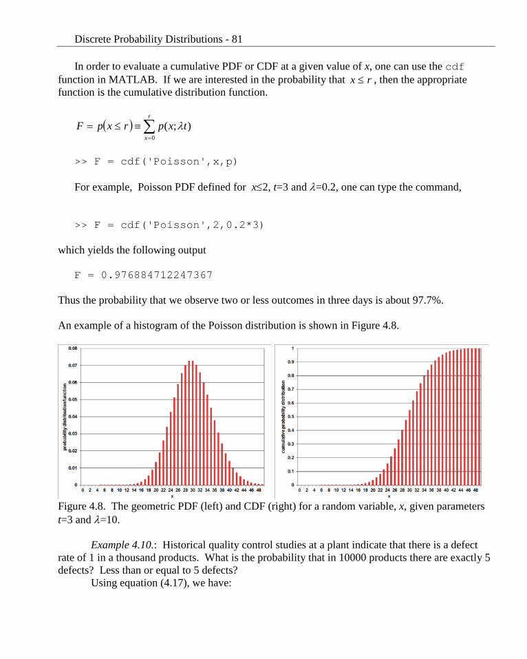
Thus the probability that we observe two or less outcomes in three days is about 97.7%. An example of a histogram of the Poisson distribution is shown in Figure 4.8.

Figure 4.8. The geometric PDF (left) and CDF (right) for a random variable, x, given parameters t=3 and λ=10.

Example 4.10.: Historical quality control studies at a plant indicate that there is a defect

rate of 1 in a thousand products. What is the probability that in 10000 products there are exactly 5 defects? Less than or equal to 5 defects?

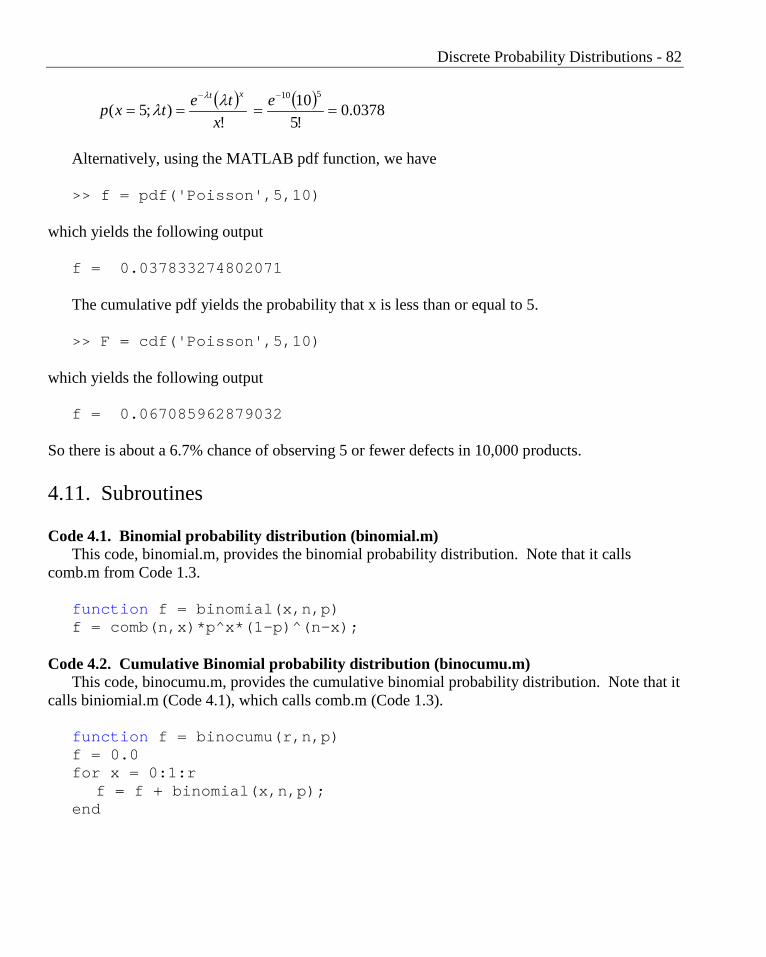
Using equation (4.17), we have:


( ) ( ) 0378.0!510

!);5(

510

====−− e

xtetxp

xt λλλ

Alternatively, using the MATLAB pdf function, we have >> f = pdf('Poisson',5,10)

which yields the following output f = 0.037833274802071 The cumulative pdf yields the probability that x is less than or equal to 5. >> F = cdf('Poisson',5,10)

which yields the following output f = 0.067085962879032

So there is about a 6.7% chance of observing 5 or fewer defects in 10,000 products.

4.11. Subroutines

Code 4.1. Binomial probability distribution (binomial.m) This code, binomial.m, provides the binomial probability distribution. Note that it calls

comb.m from Code 1.3. function f = binomial(x,n,p) f = comb(n,x)*p^x*(1-p)^(n-x);

Code 4.2. Cumulative Binomial probability distribution (binocumu.m)

This code, binocumu.m, provides the cumulative binomial probability distribution. Note that it calls biniomial.m (Code 4.1), which calls comb.m (Code 1.3).

function f = binocumu(r,n,p) f = 0.0 for x = 0:1:r



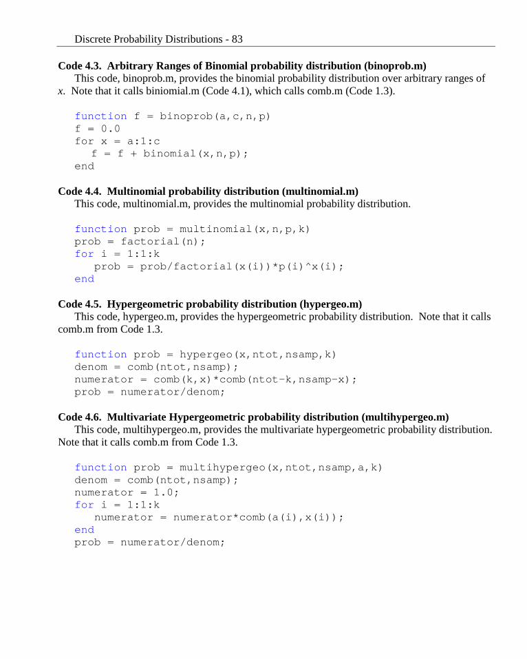
Code 4.3. Arbitrary Ranges of Binomial probability distribution (binoprob.m) This code, binoprob.m, provides the binomial probability distribution over arbitrary ranges of

x. Note that it calls biniomial.m (Code 4.1), which calls comb.m (Code 1.3). function f = binoprob(a,c,n,p) f = 0.0 for x = a:1:c


Code 4.4. Multinomial probability distribution (multinomial.m) This code, multinomial.m, provides the multinomial probability distribution. function prob = multinomial(x,n,p,k) prob = factorial(n); for i = 1:1:k prob = prob/factorial(x(i))*p(i)^x(i); end

Code 4.5. Hypergeometric probability distribution (hypergeo.m) This code, hypergeo.m, provides the hypergeometric probability distribution. Note that it calls

comb.m from Code 1.3.

function prob = hypergeo(x,ntot,nsamp,k) denom = comb(ntot,nsamp); numerator = comb(k,x)*comb(ntot-k,nsamp-x); prob = numerator/denom;

Code 4.6. Multivariate Hypergeometric probability distribution (multihypergeo.m) This code, multihypergeo.m, provides the multivariate hypergeometric probability distribution.

Note that it calls comb.m from Code 1.3. function prob = multihypergeo(x,ntot,nsamp,a,k) denom = comb(ntot,nsamp); numerator = 1.0; for i = 1:1:k numerator = numerator*comb(a(i),x(i)); end prob = numerator/denom;


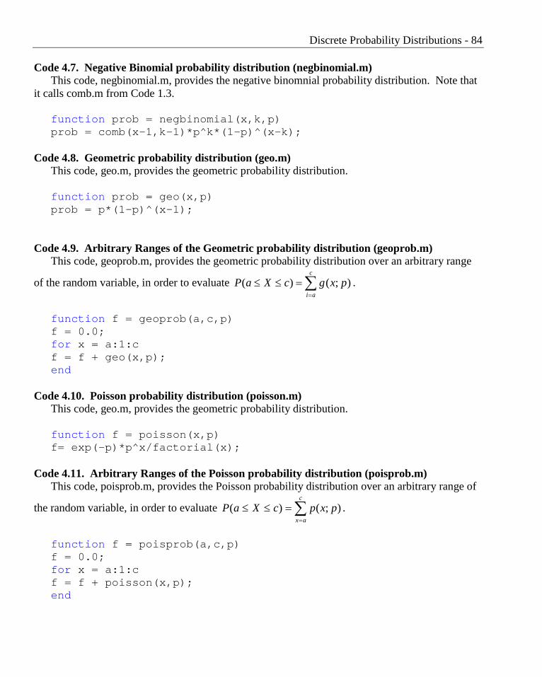
Code 4.7. Negative Binomial probability distribution (negbinomial.m) This code, negbinomial.m, provides the negative binomnial probability distribution. Note that

it calls comb.m from Code 1.3.

function prob = negbinomial(x,k,p) prob = comb(x-1,k-1)*p^k*(1-p)^(x-k);

Code 4.8. Geometric probability distribution (geo.m) This code, geo.m, provides the geometric probability distribution.

function prob = geo(x,p) prob = p*(1-p)^(x-1);

Code 4.9. Arbitrary Ranges of the Geometric probability distribution (geoprob.m) This code, geoprob.m, provides the geometric probability distribution over an arbitrary range

of the random variable, in order to evaluate ∑=

=≤≤c

aipxgcXaP );()( .

function f = geoprob(a,c,p) f = 0.0; for x = a:1:c f = f + geo(x,p); end

Code 4.10. Poisson probability distribution (poisson.m)

This code, geo.m, provides the geometric probability distribution. function f = poisson(x,p) f= exp(-p)*p^x/factorial(x);

Code 4.11. Arbitrary Ranges of the Poisson probability distribution (poisprob.m) This code, poisprob.m, provides the Poisson probability distribution over an arbitrary range of

the random variable, in order to evaluate ∑=

=≤≤c

axpxpcXaP );()( .

function f = poisprob(a,c,p) f = 0.0; for x = a:1:c f = f + poisson(x,p); end


4.12. Problems

Problems are located on the course website.

chapter 4. discrete probability...

Documents